the Creative Commons Attribution 4.0 License.
the Creative Commons Attribution 4.0 License.
 | 07 Jan 2022
Interaction between Atlantic cyclones and Eurasian atmospheric blocking drives wintertime warm extremes in the high Arctic
Rodrigo Caballero
Gunilla Svensson
Lukas Papritz
Atmospheric blocking can influence Arctic weather by diverting the mean westerly flow and steering cyclones polewards, bringing warm, moist air to high latitudes. Recent studies have shown that diabatic heating processes in the ascending warm conveyor belt branch of extratropical cyclones are relevant to blocking dynamics. This leads to the question of the extent to which diabatic heating associated with mid-latitude cyclones may influence high-latitude blocking and drive Arctic warm events. In this study we investigate the dynamics behind 50 extreme warm events of wintertime high-Arctic temperature anomalies during 1979–2016. Classifying the warm events based on blocking occurrence within three selected sectors, we find that 30 of these events are associated with a block over the Urals, featuring negative upper-level potential vorticity (PV) anomalies over central Siberia north of the Ural Mountains. Lagrangian back-trajectory calculations show that almost 60 % of the air parcels making up these negative PV anomalies experience lifting and diabatic heating (median 11 K) in the 6 d prior to the block. Further, almost 70 % of the heated trajectories undergo maximum heating in a compact region of the mid-latitude North Atlantic, temporally taking place between 6 and 1 d before arriving in the blocking region. We also find anomalously high cyclone activity (on average five cyclones within this 5 d heating window) within a sector northwest of the main heating domain. In addition, 10 of the 50 warm events are associated with blocking over Scandinavia. Around 60 % of the 6 d back trajectories started from these blocks experience diabatic heating, of which 60 % undergo maximum heating over the North Atlantic but generally closer to the time of arrival in the block and further upstream relative to heated trajectories associated with Ural blocking. This study suggests that, in addition to the ability of blocks to guide cyclones northwards, Atlantic cyclones play a significant role in the dynamics of high-latitude blocking by providing low-PV air via moist-diabatic processes. This emphasizes the importance of the mutual interactions between mid-latitude cyclones and Eurasian blocking for wintertime Arctic warm extremes.
- Article
(16649 KB) - Full-text XML
-
Supplement
(286 KB) - BibTeX
- EndNote


The positive trend observed in global-mean surface temperatures is unequally distributed, with greater and more rapid surface warming seen over the Northern Hemisphere high-latitude regions. This phenomenon, specifically observed in winter during recent decades, is known as Arctic amplification (e.g., Serreze and Barry, 2011; Cohen et al., 2014). As a result, dramatic changes have been seen, such as Arctic sea-ice loss and decline in snow cover and continental ice sheets (e.g., Richter-Menge and Co-Authors, 2020; Simmonds, 2015).
The mechanisms responsible for Arctic amplification are still under discussion. A wide range of local and remote processes have been identified. Local processes comprise snow- and ice-albedo feedbacks (e.g., Screen and Simmonds, 2010a; Pithan and Mauritsen, 2014), enhanced ocean–atmosphere heat exchanges (e.g., Screen and Simmonds, 2010b; Boisvert et al., 2016), temperature feedbacks and related changes of water vapor content and cloud cover (e.g., Serreze et al., 2012), and circulation changes within the Arctic (e.g., Sorteberg and Walsh, 2008; Ding et al., 2017), while remote processes include increased oceanic (Årthun et al., 2016) and atmospheric poleward transport of heat and moisture (e.g., Tjernström et al., 2015; Woods and Caballero, 2016; Naakka et al., 2019) mediated by anomalous large-scale circulation patterns outside the Arctic (e.g., Graversen, 2006; Woods et al., 2013; Liu and Barnes, 2015; Baggett et al., 2016). In particular, the northward moisture transport from lower latitudes has emerged as a significant modulator of the surface energy balance in the Arctic, where intrusions of warm and humid air masses replace the cold and clear state by a warm and opaque state (e.g., Francis and Hunter, 2006; Doyle et al., 2011; Woods and Caballero, 2016; Mortin et al., 2016; Pithan et al., 2018).
Many of the aforementioned processes are highly episodic. For example, increasing northward moisture transport is the result of an increasing number of a few but intense moisture transport events, mainly occurring over the Pacific and Atlantic (Woods et al., 2013; Liu and Barnes, 2015; Naakka et al., 2019). Likewise, short-lived warm extremes have a disproportionate contribution to sea-ice variability and loss (Boisvert et al., 2016; Cullather et al., 2016; Woods and Caballero, 2016; Moore, 2016; Binder et al., 2017; Kim et al., 2017; Wernli and Papritz, 2018). For this reason we focus here on episodic wintertime warm extremes.
1.1 Weather systems and importance of blocking
Northward moisture transport and Arctic warm extremes are favored by specific circulation patterns. The large-scale flow associated with intense wintertime moisture transport events and warm surface temperature extremes in the high Arctic is characterized by a poleward shift of the jet and a dipole in geopotential height over the North Atlantic, with a high over northern Eurasia and a low either in the high Arctic or along Greenland's east coast (Messori et al., 2018; Papritz, 2020; Fearon et al., 2020). This configuration is conducive to the transport of mid-latitude air masses poleward across the Nordic Seas and deep into the Arctic basin. Such events are further favored by the absence of a widespread high-pressure ridge over the Arctic Ocean (Nygård et al., 2019).
The positive and negative geopotential height anomalies are the result of collocated anomalies in the frequency and pathways of particular weather systems. This includes the frequent northward displacement of the tracks of extratropical cyclones towards Greenland's east coast and extending into (or locally created in) the high Arctic (Sorteberg and Walsh, 2008; Messori et al., 2018; Fearon et al., 2020), anticyclonic Rossby wave breaking over the North Atlantic (Liu and Barnes, 2015), and blocking over Scandinavia or the Barents Sea and the Urals (Woods et al., 2013; Papritz, 2020). Furthermore, links between indices of climate variability modes, specifically the positive phase of the North Atlantic Oscillation (NAO+), and the increased occurrence of cyclones in the Arctic (Simmonds et al., 2008) or in the North Atlantic (Pinto et al., 2009), as well as links between NAO+, Ural blocking and an enhanced northward moisture transport (Luo et al., 2017; Gimeno et al., 2019), have been emphasized. These circulation anomalies are often concomitant, and a strong interplay between the cyclones and blocks has been established, where, e.g., the path of northward-traveling cyclones is steered by blocking (Madonna et al., 2020; Papritz and Dunn-Sigouin, 2020).
Recent studies have highlighted blocking as a key driver of surface temperature extremes both in mid-latitudes (Pfahl et al., 2014; Trigo et al., 2004; Zschenderlein et al., 2019) and in the Arctic (Tyrlis et al., 2019; Papritz, 2020).
Blocks can cause surface warming, locally via adiabatic compression due to subsidence (Pfahl and Wernli, 2012; Binder et al., 2017; Ding et al., 2017) and in summer also enhanced incident shortwave radiation (Wernli and Papritz, 2018), as well as remotely via the persistent transport of warm and humid air masses along the periphery of the blocks (Woods et al., 2013; Papritz and Dunn-Sigouin, 2020).
In particular, Ural blocking has been associated with Arctic sea-ice loss as well as the so-called warm-Arctic–cold-Eurasian (WACE) temperature pattern (Luo et al., 2016b, a; Tyrlis et al., 2019; Kim et al., 2021). Specifically, Gong and Luo (2017) show that Ural blocking is an important amplifier of sea-ice loss in the Barents–Kara seas (BKS) via increased surface air temperature (SAT) anomalies over BKS concurrent with the enhanced northward moisture flux convergence and the intensified downward longwave radiation. The in-phase correlation between BKS SAT anomalies and anticyclonic anomalies over the Ural region is also noted by Kim et al. (2021), emphasizing the major role of horizontal temperature advection in driving the observed WACE patterns, whereas the budget analysis reveals a canceling of the warming by diabatic and adiabatic cooling induced by Ural blocking.
1.2 Blocking formation mechanisms
Given the importance of blocking for Arctic warm events, there has been a growing interest in examining the mechanisms behind the formation and maintenance of high-latitude blocks, not least because of large biases in the representation of blocking in climate models (e.g., Tibaldi and Molteni, 1990; Woollings et al., 2018). The dynamical mechanisms driving the formation and maintenance of blocks are generally not fully understood, and as a consequence, there is no agreement on a unique definition of blocking. Thus, a range of different blocking identification methods exists, each one emphasizing different characteristics of blocking such as flow reversal or upper-level potential vorticity (PV) anomalies (e.g., Tibaldi and Molteni, 1990; Pelly and Hoskins, 2003; Schwierz et al., 2004; Croci-Maspoli et al., 2007; Tyrlis and Hoskins, 2008).
Classical, dry-dynamical theories for blocking include global theories emphasizing the influence of planetary-scale dynamics including Rossby wave trains and their interaction with the background flow and topography (e.g., Grose and Hoskins, 1979; Hoskins and Karoly, 1981; Reinhold and Pierrehumbert, 1982), as well as local theories pointing out the importance of Rossby wave breaking (Masato et al., 2012) and slow-moving synoptic-scale eddies located upstream of blocks (Colucci, 1985) in blocking dynamics. Coupling of low- and high-frequency forcing and their relative importance are also highlighted by Nakamura et al. (1997). As for Ural blocking, Wang et al. (2021) emphasize the occurrence and competition of diverse processes responsible for the evolution of the block; the initial wave activity growth upstream is initiated by local baroclinic growth and wave propagation, whereas barotropic advection of wave activity, mainly extracted upstream, dominates the growth downstream and dominates in the growth stage of the evolution of the block. Furthermore, they show that the dissipation of the block is an aftereffect of decaying wave propagation and advection and a diabatic dampening due to radiative cooling in the free atmosphere.
In general, blocking can be characterized as an extended ridge, represented by high-potential-temperature (θ) anomalies on the dynamical tropopause (PV isosurface) or low-PV anomalies on an isentrope. This latter characterization of blocking is particularly useful as it relates blocking to conserved quantities (PV, θ) in adiabatic flow (Hoskins et al., 1985; Woollings et al., 2018). Despite the quasi-stationary nature of the blocking patterns, often the upper-level flow in blocks is highly dynamic. For example, low-PV air in the upper troposphere is constantly refueled via the isentropic advection of air from regions with climatologically lower PV values (Hoskins et al., 1985).
In addition to the dry-dynamical processes described above, recent studies have emphasized the importance of moist processes associated with the cross-isentropic transport of low-PV air into the blocking region. More precisely, cloud-diabatic processes in the strongly ascending warm conveyor belt of extratropical cyclones have been found to contribute substantially to the formation and maintenance of the negative upper-level PV anomaly by transporting low-PV air cross-isentropically from the lower troposphere into the upper troposphere (e.g., Croci-Maspoli and Davies, 2009; Madonna et al., 2014, 2015; Pfahl et al., 2015; Steinfeld and Pfahl, 2019). Moist processes are important especially in the early stage of the blocking life cycle and can contribute to ridge amplification and faster growth (Pfahl et al., 2015; Steinfeld et al., 2020). Numerical experiments further show that turning off the latent heating upstream of blocks clearly reduces the cross-isentropic transport of low-PV air to the upper troposphere and can even prevent blocking formation (Steinfeld et al., 2020). However, in the mature stage with favorable background conditions, such as a pre-existing ridge, the absence of latent heating has a smaller impact on the block.
Our goal in this study is to investigate the dynamics behind wintertime Arctic warm extremes. Specifically, we aim to address the following questions.
-
What is the role of blocking in driving these extreme warm events?
-
Are there regional differences in the circulation patterns among the different warm extremes?
-
How important are diabatic processes in driving the blocks?
-
How do cyclones and blocks interact during these warm events?
As discussed in Sect. 2, which provides an overview of the data and methods used in this study, we focus on the top 50 high wintertime Arctic warm extreme events previously examined in Messori et al. (2018). Our results are presented in four sections (Sects. 3–6), beginning with an illustrative example of a sequence of three temporally close warm extreme events and their dynamical drivers (Sect. 3). Section 4 investigates the role of blocking for all of the 50 warm extremes, presented in their corresponding event clusters. Subsequently, the dynamics of the blocking events are discussed in Sect. 5, including an examination of blocking trajectory characteristics. This is followed in Sect. 6 by a discussion of the interaction between mid-latitude cyclones and the blocks associated with warm events. We finalize our study with a discussion in Sect. 7 and summarize our key findings in the concluding Sect. 8.
The analysis in this study is based on 6-hourly ERA-Interim reanalysis data (Dee et al., 2011) provided by the European Centre for Medium-Range Weather Forecasts (ECMWF). We focus on the Northern Hemisphere mid-latitudes and high latitudes for the extended winter season, November through March (NDJFM). The original spatial resolution of ERA-Interim, approximately 80 km, vertically on 60 model levels, is used for most parameters, although for some (potential vorticity and geopotential height) we use data horizontally interpolated to a grid and on pressure levels in the vertical. Anomalies are defined as deviations from the calendar-monthly climatology averaged over the 38-year period used in this study (1979–2016) unless otherwise mentioned.
2.1 High-Arctic warm extreme events
We focus on the same 50 extreme warm events of wintertime high-Arctic 2 m temperature (T2m) anomalies previously identified in Messori et al. (2018). We briefly summarize the identification method here for the reader's convenience. Warm anomalies are computed with respect to a daily climatology from which the non-linear warming trend seen in the Arctic (Cohen et al., 2014) is removed by applying a 21 d running window on a 9-year running-mean calendar-day climatology. Mean Arctic temperature anomalies are then obtained by area weighting and averaging the daily values over the polar cap (>80∘ N). Finally, aiming at retaining persistent deviations from the climatology and avoiding double counting of events, a further 5 d running-mean filter is implemented and the most anomalous days with at least 1-week time difference are chosen. The top 50 warm extremes are then selected, ranked by decreasing temperature anomaly. In the rest of the paper, individual events are identified by their rank (e.g., event 3 is the third-warmest event).
It is worth mentioning that the four most extreme events (January 2006, March 1992, November 2016 and January 2000) are well distinguished from the other extremes, obtaining T2m anomalies greater than 10 K. A detailed overview of the 50 warm extreme events is presented in Sect. 4.
2.2 Blocking identification
Quasi-stationary atmospheric blocks are identified using a PV-index method, which is based on upper-level (150–500 hPa) negative vertically averaged PV anomalies, following the algorithm by Schwierz et al. (2004). The 6-hourly vertically averaged PV (hereafter VAPV) anomaly fields, computed with respect to the monthly climatology and temporally smoothed using a 2 d running-mean filter, are used as input data for the blocking index calculations. This dynamically based method captures the core of the PV anomaly located in the upper troposphere, enabling a more comprehensive analysis of its dynamical characteristics, lifetime, maintenance and evolution.
A temporal and spatial overlapping criterion is used to find each blocking life cycle. Here, at each time step, blocking masks are determined from the VAPV field where it falls below a threshold value of −1.3 pvu (1 pvu (potential vorticity unit) ), which is based on previous studies (e.g., Croci-Maspoli et al., 2007; Pfahl et al., 2015; Steinfeld and Pfahl, 2019; Lenggenhager and Martius, 2020). Then, these masks are connected in time if at two consecutive time steps they overlap by at least 70 %. We then identify a block if the temporally connected masks persist for at least 5 d. Applying the blocking algorithm for the whole study time period results in fields indicating the presence of a block at each grid point and 6-hourly time step and its unique identification number.
Additionally, the life stage of each individual blocking life cycle is quantified by the D index. This index attains values between 0 and 1 and is defined as follows:
Figure 1 illustrates the blocking identification method applied to event 9, where the black box in Fig. 1a highlights the identified upper-level blocking region in which the above-mentioned criteria are fulfilled. Within this box, the elevated tropopause coincides with positive and negative geopotential height and PV anomalies, respectively. The block north of the Ural Mountains in Fig. 1b has a northwestward tilt relative to the region of positive sea-level pressure (SLP) anomalies observed at the surface, and it is accompanied by a northward flow of moist air to the west of the block.
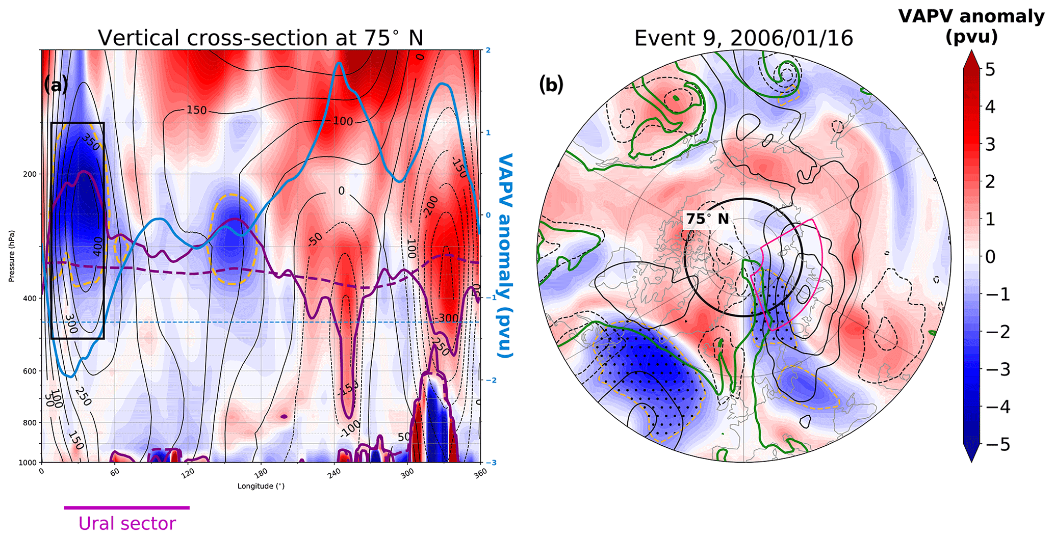
Figure 1An illustrative example of the blocking identification algorithm for 12:00 UTC on 16 January 2006, 1 d prior to event 9. (a) Vertical cross section along 75∘ N showing PV anomaly (shading, −1.3 pvu isoline highlighted by orange, dashed line), tropopause at 2 pvu (purple solid), climatological tropopause (purple dashed) and geopotential height anomalies (black contours every 50 gpm, geopotential height meters). Also shown is the VAPV anomaly and the threshold of −1.3 pvu (light-blue solid and dashed contour, respectively; scale on the right). The Ural sector is indicated by a magenta horizontal line below the figure, and the black box highlights the identified Ural block. Note the logarithmic scale in the vertical. (b) VAPV anomaly (shading) overlaid with SLP anomalies (hPa, black contours every 10 hPa, negative values dashed, zero contour not shown), total column water (5 kg m−2 isoline, green solid) and VAPV anomaly (−1.3 pvu, orange dashed). Dotted areas show the identified blocking regions, and the black line and the magenta box indicate the location of the cross section in panel (a) and the Ural sector, respectively.
2.3 Trajectory calculation
To further quantify the importance of different processes leading up to the identified blocks, we compute 10 d three-dimensional kinematic back trajectories using the Lagrangian Analysis Tool (LAGRANTO; Sprenger and Wernli, 2015). LAGRANTO calculates trajectories x(t) using three-dimensional wind fields on reanalysis model levels and a 30 min computational time step. Trajectory starting positions are selected based on the blocking mask, re-gridded to match the same horizontal resolution as the reanalysis data. More specifically, trajectories are initialized at every grid point within the blocking mask, horizontally on an equidistant 80 km×80 km grid and vertically every 50 hPa between 500 and 150 hPa. Starting times are daily at 12:00 UTC. For the analysis, however, blocking preceding a warm event is being represented by 1 specified day within the narrow −3 to −1 d window before each warm event, as will be explained in Sect. 4. Only starting points with <1 pvu are used in the interest of studying tropospheric air. Additionally, various quantities are traced along each trajectory, such as PV, θ, PV anomaly (here calculated with respect to the 10 d running-mean climatology) and specific humidity (Q).
2.4 Cyclone tracking method
Cyclone tracks are calculated using the algorithm developed by Murray and Simmonds (1991). Tracking is done on mean sea-level pressure data (MSLP) north of 30∘ N. Same instruction parameters as listed in Table 1 in the study by Uotila et al. (2009) are selected. Only cyclones lasting for at least 24 h are included in this study.
Before proceeding to the climatological analysis of the dynamics behind the extreme warm events, a case study for winter 2005/06 is presented to illustrate the interaction between Atlantic cyclones and Eurasian blocking in the lead-up to Arctic warm extremes. The winter 2005/06 in Europe was dominated by blocking regimes, especially in January 2006 with cold anomalies observed over continental Europe and Russia (Croci-Maspoli and Davies, 2009), which were accompanied by periods of heavy snowfall over central Europe (Pinto et al., 2007). Conversely, positive DJF T2m anomalies occurred over the North Atlantic, North America and the polar regions (Croci-Maspoli and Davies, 2009).
The algorithm of Messori et al. (2018) identifies three high-Arctic warm extreme events during January 2006: events 28, 9 and 1, occurring on the 8th, 17th and 24th and attaining a high-Arctic averaged T2m anomaly of 8, 9 and 12 K respectively (see Fig. 2). It is clear that though they are classified as individual events, the three peaks are actually local maxima within a constantly increasing temperature anomaly until reaching the most extreme event. The analysis below suggests that they could also be thought of as sub-events in a single, persistent warm extreme supported by two separate blocking events that manifest in two different sectors, one near the Ural Mountains and another over Scandinavia; these sectors are further discussed in Sect. 4.
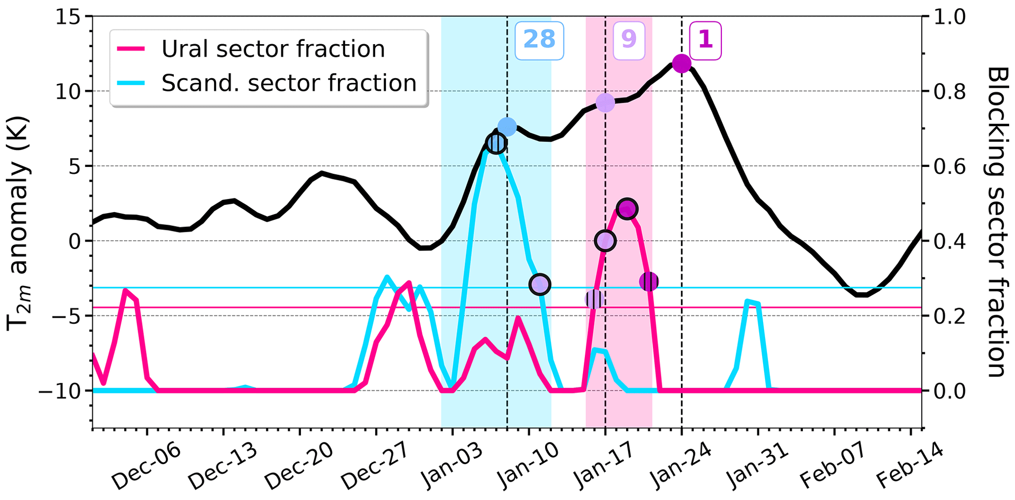
Figure 2Daily variation of high-Arctic area-averaged T2m anomalies (black) and blocking fraction (based on the area fraction of the sector that intersects with a block as identified by the algorithm described in Sect. 2) area averaged over the Ural (magenta) and Scandinavian (cyan) sectors during 1 December–15 February 2006. Three Arctic warm events are marked with vertical black dashed lines with event ID indicated in boxes to the right of each event line. The magenta and cyan horizontal thin lines mark the 90th percentile thresholds of the daily blocking fractions, and the lifetime of two blocks is indicated by magenta and cyan shading for Ural and Scandinavian blocks, respectively. The timings of the maximum blocking fraction within 3 (corresponding to the time of trajectory initialization) and 6 d prior to each event are shown by hatched and solid circles, respectively, where light-blue circles refer to event 28, light-purple markers to event 9 and magenta markers to event 1. The x ticks are shown at 12:00 UTC.
3.1 Synoptic situation
On 3 January (Fig. 3a), a ridge (high θ2 pvu values) extends over the North Atlantic and further eastward. An upper-level block is identified northwest of the United Kingdom (white-dotted shaded region). Two days later (Fig. 3d), the upper-level block has moved northeastwards and now extends over Scandinavia. Meridional flow in the North Atlantic prevails, bringing warm and moist air northwards, driven by the dipole in the SLP field. Two days later ( d, Fig. 3g), the block maintains its position over Scandinavia, and the moist and warm air continues to penetrate deeper into the Arctic. The peak in blocking fraction in the Scandinavian sector (Fig. 2) occurs at the same time. At the peak of the warm event (Fig. 3j), the block is still located over Scandinavia and steers the flow northwards but is then slowly decaying (see Fig. 2) and moving southwards (not shown).

Figure 3Synoptic situation prior to three warm extreme events (columns) between 3 and 24 January 2006 at 12:00 UTC at lags −5, −3, −1 and 0 d relative to each warm event (rows). Panels (a)–(l) show potential temperature (θ) on the dynamical tropopause, defined by the 2 pvu isosurface (shading), SLP (hPa, black contours every 10 hPa, solid for SLP>1000 hPa), total column water (thick black solid for 5 kg m−2) and T2m (purple solid at 0 ∘C). White-dotted areas indicate regions with identified blocks. Magenta and red boxes indicate the Ural (h, f) and Scandinavian (g) blocking sectors, respectively. Panels (m)–(o) show T2m anomalies (shading) and SLP contours at 12:00 UTC of each warm event (lag 0 d). The black circle shows the latitude line at 80∘ N.
Three days after the first peak, on 12 January, a new event begins (Fig. 3b). The Scandinavian block is replaced by a low-pressure system, and the remaining block (white-dotted region over Poland) directs the flow around the Urals and enters into the Arctic over the Barents and Kara seas. However, 2 d later (Fig. 3e) the high over the Urals is strengthened and a low-pressure center is formed east of Greenland. At this time there is no substantial blocking identified (Fig. 2). The meridional flow strengthens as a consequence of the stronger dipole over the North Atlantic, favoring deep penetration of warm and moist air into the high Arctic at lag −1 d (Fig. 3h). Note that a new block is identified over the Arctic Ocean northeast of Scandinavia (dotted area, the Ural sector is shown in magenta). The upper-level block tilts northwestward from the surface high pressure over the Urals and northern Siberia (see also Fig. 1 and discussion in Sect. 2.2). The block expands eastwards, covering large parts of the Ural sector at the day of the warm event (Figs. 3k and 2), and the northwestward tilt remains. A strong positive response in the temperature anomaly is also seen to the north/northwest of the block and a negative one to the south/southeast of the block (Fig. 3n), resembling the WACE pattern.
The next event occurs 1 week after the second temperature anomaly peak, also influenced by the same established Ural block. The peak in the Ural sector fraction reaches its maximum value 5 d prior to the warmest event (see Fig. 2), after which the Ural sector fraction decreases such that 3 d prior to event 1 a Eurasian block is no longer detected (Fig. 3f). However, the northward advection of warm and moist air continues with the main pathway east of Greenland (Fig. 3c, f and i). After this period of increased blocking activity over Eurasia, the temperature anomaly decreases (see Fig. 2) as the flow becomes more zonal (not shown).
The spatial distribution of the T2m anomaly at the time of the extremes (Fig. 3m–o) shows a dipole between anomalously cold Eurasia and warm Atlantic and Arctic, and the negative anomalies coincide with contours of higher SLP, further supporting the findings in Croci-Maspoli and Davies (2009).
3.2 Linkage between Atlantic cyclones and blocks over Eurasia associated with the three warm events in January 2006
To explore whether there is a link between the identified blocks and cyclones, we present three sets of back trajectories (Fig. 4) initialized from the two identified Eurasian blocks – the Scandinavian block 1 d prior to event 28 (first column) – and from the Ural block influencing both of the last two events – 1 d prior to event 9 (second column) and 3 d before event 1 (last column) – with times identical to the synoptic situation presented in Fig. 3g, h and f, respectively. At the time of trajectory initialization for all three events (see Fig. 4a–c), a narrow band of moist air is intruding into the Arctic west of the block. Also, we consider cyclones and the locations of the trajectories at the time of maximum heating. Note that only trajectories that experience diabatic heating (substantial increase in θ) are shown, constituting 52 %, 73 % and 5 % of all computed trajectories for each of the three events, respectively. A more detailed definition of the trajectory classification is presented later in Sect. 5.1.
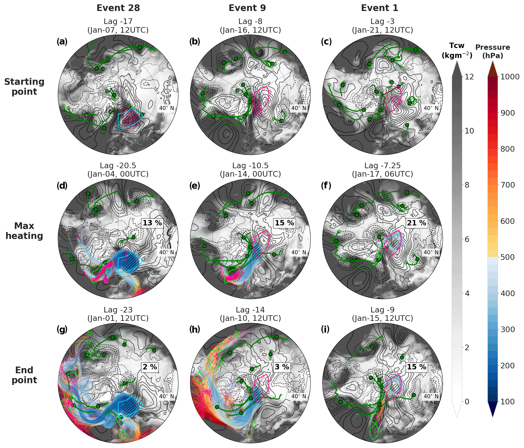
Figure 4Six day back trajectories initialized from the blocks (black hatched regions, first row) prior to the three warm events (columns). Rows indicate the trajectory locations (pink dots) at the starting point (a–c), the time of maximum diabatic heating (d–f) and the end point (g–i). The dates for which the panels are valid are denoted by lag days relative to the peak of the warmest event 1. Furthermore, the trajectories are drawn between the valid time and the starting time, colored according to pressure. Additionally shown are total column water (gray shading, kg m−2), SLP anomalies (hPa, black contours every 5 hPa, dashed for <0 hPa, zero contour not shown), and cyclone location at valid time (green dot) and tracks (green lines). Further shown is the density of trajectories experiencing maximum heating at the valid time (green contour for 5 % (106 km2)−1). The relative percentage of all heated trajectories experiencing their maximum heating at the valid time is given in the text boxes (second and third rows). The latitude circle at 40∘ N is indicated by a black dashed line, and the magenta and blue boxes indicate the Ural and Scandinavian blocking sectors, respectively.
The majority of the back trajectories started from the Scandinavian block (Fig. 4a), 2.5 weeks prior to the most extreme event, reside at lower altitudes south of 50∘ N over eastern North America and in the North Atlantic 6 d earlier (Fig. 4g). Only 2 % of all heated trajectories (change in θ along the trajectory exceeding 2 K) experience their maximum heating (green density contours) already at this stage, mainly in the vicinity of cyclones over the eastern Pacific and southwestern North Atlantic. The air parcels experience maximum heating at various times during their journey into the blocking region, though with a peak (13 % of all heated trajectories) over the North Atlantic 3.5 d prior to arrival in the block (Fig. 4d). A few of the back trajectories that pass over the Mediterranean get heated and lifted 1 d later (not shown). After the maximum, all blocking trajectories reside in the upper troposphere for several days before reaching the block (Fig. 4a).
The remaining panels show back trajectories from the same short-lived (persisting for only 6 d) Ural block, initialized at different life stages of the block with respect to the peak of event 9 and 1. As for the event 28, most of the heated trajectories initialized at the onset stage of the Ural block (Fig. 4b), 8 d prior to event 1, reside around or south of 40∘ N in the northern part of the subtropical high over the ocean 6 d prior to arrival into the block (Fig. 4h). Also here, a small fraction of the computed trajectories experience their maximum heating at this early stage, mainly over the eastern Pacific. However, the majority of the maximum heating occurs within the North Atlantic at different times from 4 d before arrival, with a peak (15 % of all heated trajectories) observed 2.5 d prior to arrival into the blocking region (Fig. 4e). The trajectories follow a fairly coherent path and move quickly once they reach the upper troposphere. Again, the lifting occurs primarily in the vicinity of a mid-latitude cyclone, located northwest of the center of maximum heating.
In contrast, capturing only 5 % of heated trajectories initialized from the decaying stage of this Ural block 3 d prior to event 1 (Fig. 4c), the time window where the maximum heating within the North Atlantic occurs is narrowed to the first 2 d from the end points of the trajectories. Already 15 % of all trajectories experience heating over the North Atlantic 6 d prior to arrival (Fig. 4i) and 21 % a few days later (maximum peak at lag −4.25 d, Fig. 4f), after which all trajectories again reside in the upper troposphere for several days before arriving in the block. Again, we observe a cyclone located to the north of the region of maximum heating (Fig. 4f and i), which in fact is the same cyclone contributing to the late lifting in Fig. 4e, though at different times and spatial locations. This suggests that a substantial portion of the lifting for these Ural blocking trajectories is accomplished by just one cyclone in the North Atlantic. The observed negative correlation between blocking life stage and the timing of maximum heating over the North Atlantic – i.e., younger blocks experience maximum heating at later times – will be discussed more generally in Sect. 5.
In summary, we showed in this case study that two significant blocks, one over Scandinavia and one over the Urals, contributed to three close-in-time warm extreme events in January 2006, the latter of which is the most extreme in the entire observational record. Additionally, a large fraction of 6 d back trajectories traced from the blocks experienced heating, in agreement with Pfahl et al. (2015) and Steinfeld and Pfahl (2019). We also saw that the majority of the heating and lifting is accomplished by a small number of cyclones in the North Atlantic.
Our case study (Sect. 3) highlights the importance of Ural and Scandinavian blocking for some of the most extreme Arctic warm events in the observational record. This raises the question of whether blocking plays a similar role in all the top-50 Arctic warm extreme events introduced in Sect. 2.1. We address that question in this section. We start by examining the 50 events collectively and assess whether or not they were preceded by significant blocking, and then proceed to classify the events by the type of blocking observed. Additionally, we discuss events that are temporally close to each other and their relation to blocks.
Figure 5a shows composite VAPV anomalies for all 50 events, averaged over the 3 d preceding the peak of the events. The composite shows a prominent negative anomaly in the Ural sector and a weaker negative anomaly over Scandinavia, suggesting that blocking in these regions is indeed a common feature to many of the events. The corresponding SLP anomalies (black contours) show a pattern consistent with that shown in Messori et al. (2018), with a high over Siberia and the Barents and Kara seas and a low over Greenland, conducive to advection of warm, moist air into the high Arctic, as indicated by values of total column water vapor typical for mid-latitudes penetrating into the Arctic.
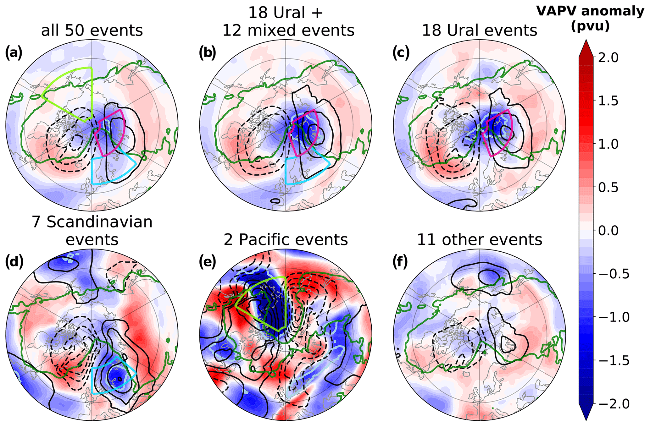
Figure 5Circulation patterns observed during warm extremes shown as time mean composites over days −3 to −1 prior to the warm events for (a) all 50 extreme events; (b) 30 events with Ural blocking, comprised of 18 pure Ural events and 12 events within the mixed cluster; (c) 18 pure Ural events; (d) 7 pure Scandinavian events; (e) 2 Pacific events; and (f) remaining 11 events belonging to the other cluster. Shown are VAPV anomalies (pvu, shading) overlaid with SLP anomalies (hPa, black contours every 5 hPa, dashed for <0 hPa, zero line not shown), total column water (green solid isoline for 5 kg m−2), and blocking frequency for the events and respective time steps involved in each composite (light-blue solid contour for 33 %). The colored boxes in panel (a) show the Ural (magenta), Scandinavian (blue) and Pacific (light green) sectors.
Detailed inspection of VAPV maps for each individual event shows considerable variability among events; however, some events feature isolated VAPV anomalies over the Urals and some over Scandinavia, and some feature an extended anomaly covering both regions; other events show generally weak anomalies everywhere, and a small number of events show very strong negative anomalies in the Pacific sector near the Bering Strait.
To translate this subjective inspection into an objective classification of blocking types, we select three sectors capturing the locations where prominent negative VAPV anomalies are most frequently found: Ural (70–85∘ N, 20–120∘ E), Scandinavia (55–70∘ N, 0–50∘ E) and Pacific (55–85∘ N, 180–120∘ W) sector (Fig. 5a, Table 1). We then define a blocking index for each sector based on the area fraction of the sector that intersects with a block as identified by the algorithm described in Sect. 2.2. Specifically, at each 6-hourly time step we compute the total area of the grid cells within the sector belonging to a block, divide by the total sector area and take a daily mean to yield a daily sector blocking index. We then relate a warm event to a blocking in a specific sector if the corresponding sector index exceeds its 90th percentile value at some point over the 6 d prior to the warm event. For the Pacific sector, we use the 99th percentile in order to capture only the strongest blocking in this frequently blocked area.
Table 1Coordinates for the sectors used in the event clustering (left) and other defined regions used in this study (right).

This procedure partitions the 50 warm events into five distinct clusters (Figs. 5b–f and 6): three “pure” clusters (Ural, Scandinavian and Pacific, containing 18, 7 and 2 events, respectively), one mixed Ural–Scandinavian cluster (12 events) and a residual cluster of 11 other events not associated with blocking in any of the sectors. The partitioning between the Ural, Scandinavian and mixed clusters is illustrated in Fig. 6b. Note that one of the residual events (coral markers) achieves a Ural blocking index marginally above the threshold but is not classified as a Ural event because detailed examination of the VAPV anomalies for that event shows that blocking extends over the entire polar cap and Greenland, making it qualitatively different from the other 18 Ural events.
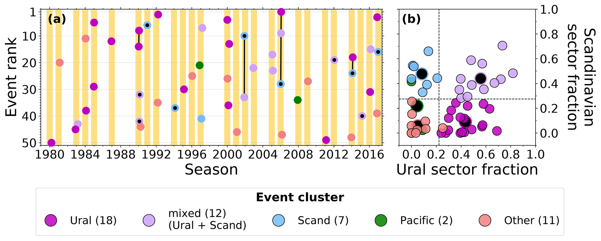
Figure 6Classification of the top 50 warm extremes by type of blocking. (a) The 50 events ordered by time and ranked by the strength of the temperature anomaly. Events discussed in the Scandinavian event analysis (Sect. 5.2) are marked with a black dot. Multiple warm events associated with a single blocking event are connected by a thick black line. Yellow bars mark the NDJFM season for each year (where, e.g., 1980 refers to winter −79 to −80). (b) Scatter plot of Ural vs. Scandinavian daily blocking index for the 50 warm events. Smaller circles mark the maximum index value in the 6 d preceding each event; large circles with black center indicate mean values for each cluster. Dashed lines show the 90th percentile threshold for each index. The marker colors refer to the five different event clusters (see legend).
Circulation patterns composited over the various clusters are shown in Fig. 5b–f. Compositing over the 18 pure Ural events (Fig. 5c) or over the 30 events with Ural blocking (i.e., combining the Ural and mixed Ural–Scandinavian clusters, Fig. 5b) shows patterns very similar to that for composites over all 50 events, though with greater amplitude. In these cases, the maximum negative VAPV anomaly is concentrated in and around the Ural sector, while the SLP anomaly shows a clear dipole straddling the pole and promoting warm advection from the North Atlantic into the high Arctic. The Scandinavian composite (Fig. 5d) has a peak VAPV anomaly over Scandinavia, as expected, while the SLP again shows a dipole structure with a high over Scandinavia, partly extending over to northern Siberia, and a low over Greenland, again promoting advection from the North Atlantic. The Pacific composite shows very strong negative VAPV anomalies over Alaska, and the SLP anomalies show a dipole with a high over Alaska and a low over eastern Siberia. This pattern supports warm advection from the North Pacific, reflected in the structure of the total column water field (green contour) showing intrusion of mid-latitude air into the Arctic from the Pacific. Note that the 30 % blocking frequency contour (light blue) nicely encloses regions of peak negative VAPV anomaly in each of the aforementioned cluster composites. Finally, the 11 residual events show weak VAPV and SLP anomalies with a structure similar to that in the pure Ural composite. This resemblance suggests that many of the residual events are in fact weak Ural events, and might have been classified as such had we used a lower VAPV threshold in the blocking identification algorithm. However, in the remainder of the paper we focus on the higher-amplitude events in the other clusters.
As noted in Sect. 3, our case study shows that two successive warm extremes occurring in rapid succession can in fact be driven by a single blocking event. We find that this occurs five times within our top 50 warm extremes. These five pairs of warm events (connected by black lines in Fig. 6a) all occur within 13 d of each other, and the second event is always warmer than the first. The criteria used to select the warm extremes (following Messori et al., 2018) arbitrarily stipulate that two consecutive events are considered independent if they are separated by more than 1 week. As also noted in Sect. 3, the more physically based blocking perspective taken here suggests that these pairs of events could also be thought of as single, long-lasting warm events driven by a single blocking event.
The previous section showed a strong association between blocks and extreme Arctic warm events. Here, we take a closer look at the dynamics behind these blocking events, focusing on the sources of low-PV air as identified by Lagrangian back trajectories initialized within the blocks (Sect. 2.3). Apart from quasi-adiabatic transport of low-PV air related to classical, dry-dynamical blocking formation processes as described in the introduction, in this study we are particularly interested in the contribution of diabatic heating within mid-latitude cyclones and its importance to Eurasian blocking, as in Pfahl et al. (2015); Binder et al. (2017).
5.1 Ural blocking
We focus first on blocking in the Ural sector, combining the 18 pure Ural blocks with the 12 mixed Ural–Scandinavian events (Fig. 5b). For the latter, the blocking algorithm identifies two disjoint blocking regions – one over the Urals and one over Scandinavia – in six cases; in these cases, trajectories are initialized only from the Ural block. In the remaining six cases, a single block extending over both sectors is identified. We apply an additional geographical mask in order to initialize trajectories only over the portion of the block residing over the Ural Mountains (mainly north of 60∘ N). Furthermore, a few of the pure Ural events also obtain scattered blocking regions, for which we apply the same method as described above. The exact masks used for a total of seven Ural events are shown by the footnotes after each event number in Table S1 in the Supplement (Sect. S1). Back trajectories are started at the time of maximum Ural blocking fraction within the interval 3 to 1 d before the peak of each warm event. We compute a total of 97 405 trajectories initialized 3, 2 and 1 d prior to each warm event for 12, 6 and 12 of the 30 Ural events, respectively.
Following previous work (Pfahl et al., 2015; Steinfeld and Pfahl, 2019), we assess the role of diabatic heating by examining the change in dry potential temperature (Δθ) along trajectories as follows. We identify the absolute maximum θ along the trajectory and find the (positive) difference Δθ+ between this maximum and the previous minimum θ. Similarly, we find the (negative) difference Δθ− between the absolute minimum and the subsequent maximum. If K, the trajectory is classed as “heated” and ; otherwise, the trajectory is classed as “not heated” and Δθ is set equal to either Δθ+ or Δθ−, whichever has greater absolute value.
Figure 7a shows histograms of Δθ for all 30 events using backward trajectories of increasing length; the inset panel shows the fraction of heated trajectories as a function of trajectory length. The histograms are bimodal by construction, with separate positive and negative lobes. As trajectory length increases the two modes move further apart: air parcels experience greater heating and cooling the longer they are traced. The fraction of trajectories in the heated class rises rapidly from less than 10 % at 1 d to almost 60 % (59 %, 57 323 trajectories) at 6 d but changes little thereafter, implying that 6 d is a reasonable trajectory length when considering diabatic heating effects in Ural blocking.

Figure 7Ural (first column) and Scandinavian (second column) blocking trajectory regimes and their characteristics. (a, b) Frequency distribution of maximum change in potential temperature along back trajectories initialized from Ural (a) and Scandinavian (b) blocks during 3 (blue), 5 (light blue), 6 (pink), 7 (orange) and 9 (brown) days before their arrival into the blocking region. The threshold value of Δθ=2 K is shown by the black vertical dashed line. The inset figure shows the percentages of trajectories counted in the no-heating (N, blue) and heating (H, red) regimes by increasing the length of trajectories. Figure is inspired by Steinfeld and Pfahl (2019). (c–f) Pressure evolution (hPa, shading) with potential temperature on the vertical axis of blocking trajectories within the two regimes: heating (H, in red) (c, d) and no-heating (N, in blue) (e, f), averaged within each grid box (6 h×2 K). Note the different y-axis range for the two regimes. The distribution of trajectories is shown in black lines (median in solid, thick dashed lines for the interquartile range (IQR) and the thin dashed lines for the 5th–95th percentile range). The regime separation in panels (c)–(f) is based on 6 d back trajectories. The two vertical black dashed lines in panels (c) and (d) mark the lifting window between lags −1 and −6 d.
Figure 7c shows the time evolution of θ and pressure for trajectories in the 6 d heated regime. At 6 d before arrival, air parcels are almost entirely below the 500 hPa level (warm colors), with the median trajectory (thick black line) close to 700 hPa and θ around 300 K, typical values for mid-latitude air (Hoskins et al., 1985). In the subsequent days they warm and rise into the upper troposphere. The median trajectory rises by around 300 hPa in 3 d, but the ascent rate for individual trajectories is considerably more rapid: the maximum 2 d pressure drop for these trajectories has a median value around 400 hPa (Fig. 8e). Further, the median humidity change along these trajectories is a drying of around 4 g kg−1 (Fig. 8i); condensation of this amount of water vapor yields an isobaric warming of around 10 K, comparable to the median heating of about 11 K for 6 d trajectories shown in Fig. 8a. Overall, these results are consistent with the view that diabatic heating occurs principally through latent heat release in the rising branches of cyclones (Madonna et al., 2014).
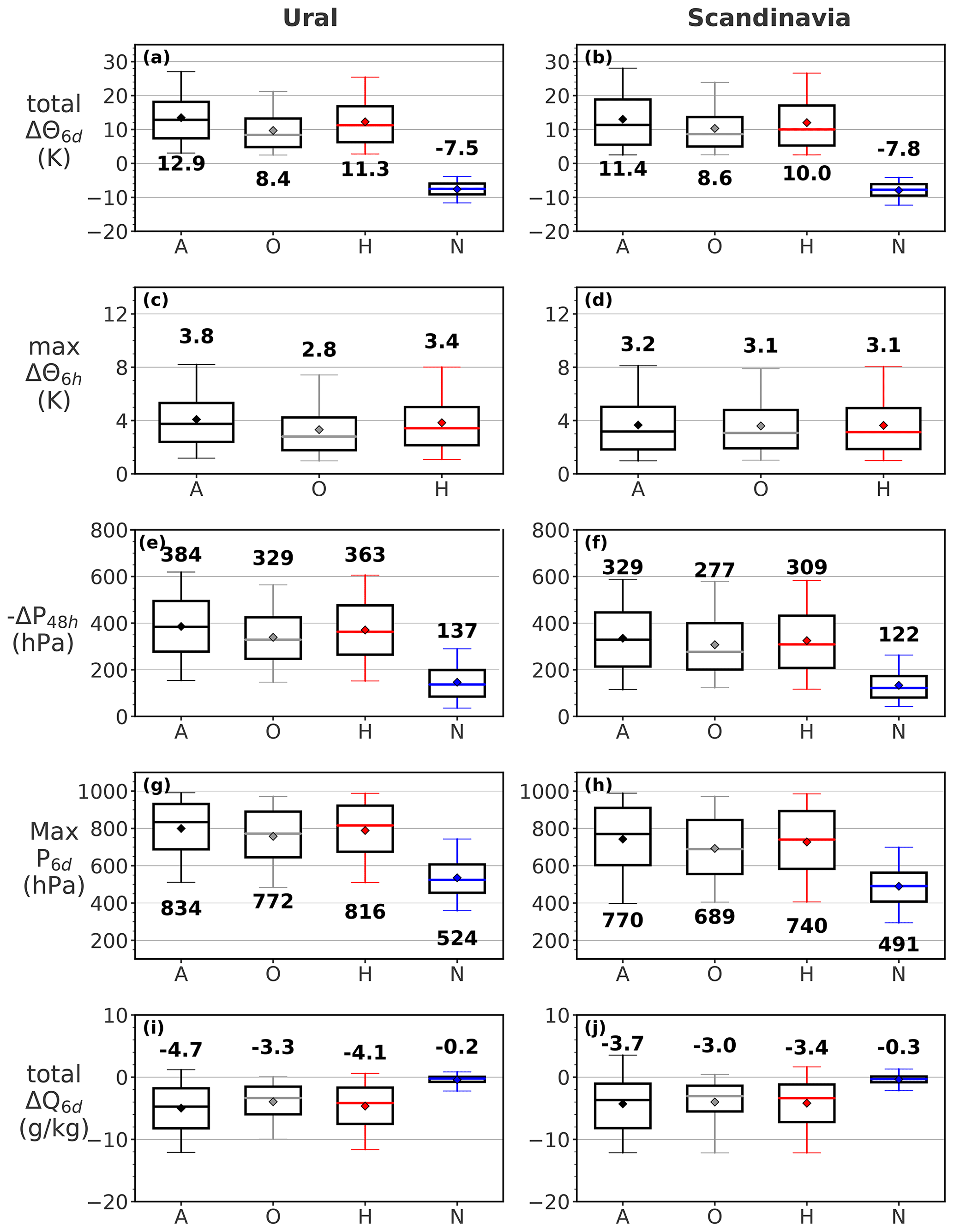
Figure 8Statistical distributions of maximum absolute change in potential temperature (K) (a, b), maximum 6-hourly change in potential temperature (K) (c, d), maximum absolute ascent (hPa) within 48 h (e, f), maximum pressure (hPa) (g, h) and maximum change in specific humidity (g kg−1) (i, j) along the 6 d back trajectories belonging to the non-heating regime (N, blue lines) and heating regime (H, red lines), initialized from both Ural (first column) and Scandinavian (second column) blocks. The heating regime is further subdivided into trajectories experiencing maximum heating in the main domain (A, black lines) and outside the domain (O, gray lines). The second row is only shown for heated trajectories. The whiskers show the 5th–95th percentile range, the box shows the interquartile range and the mean is shown as diamonds. Horizontal lines and the bold values denote the median for each distribution.
Trajectories in the no-heating regime, on the other hand, are almost entirely in the upper troposphere on day −6 (Fig. 7e); they cool diabatically at a median rate of around 1.3 K d−1 (Fig. 8a), consistent with typical radiative cooling rates in the upper troposphere, and they subside by around 140 hPa as they travel to the blocking region.
The results above show that diabatic heating is an important factor in the identified Ural blocking events, at least when tracing air parcels back for 6 d and when averaging over all 30 cases. There is considerable variability among cases, but 23 of them (77 %) have a 6 d heated fraction in excess of 40 % (Fig. 9, red markers). Cases 1 and 8 both have a very low heating fraction: less than 10 %. Interestingly, these are both cases in which a single blocking event generates two consecutive warm events (see Fig. 6). They are thus examples of long-lived blocks, where low-PV air has been recirculating for several days after diabatic heating (Steinfeld and Pfahl, 2019). Low heating fractions are also consistent with the blocks being in the decaying stage of their life cycles (e.g., Pfahl et al., 2015; Steinfeld and Pfahl, 2019), where the diabatic cooling may have a damping role and finally lead to the demise of the block (Wang et al., 2021). Averaging over the per-event defined 6 d heating fractions, we obtain a slightly lower percentage of 54 %, mainly due to the influence of these two events.
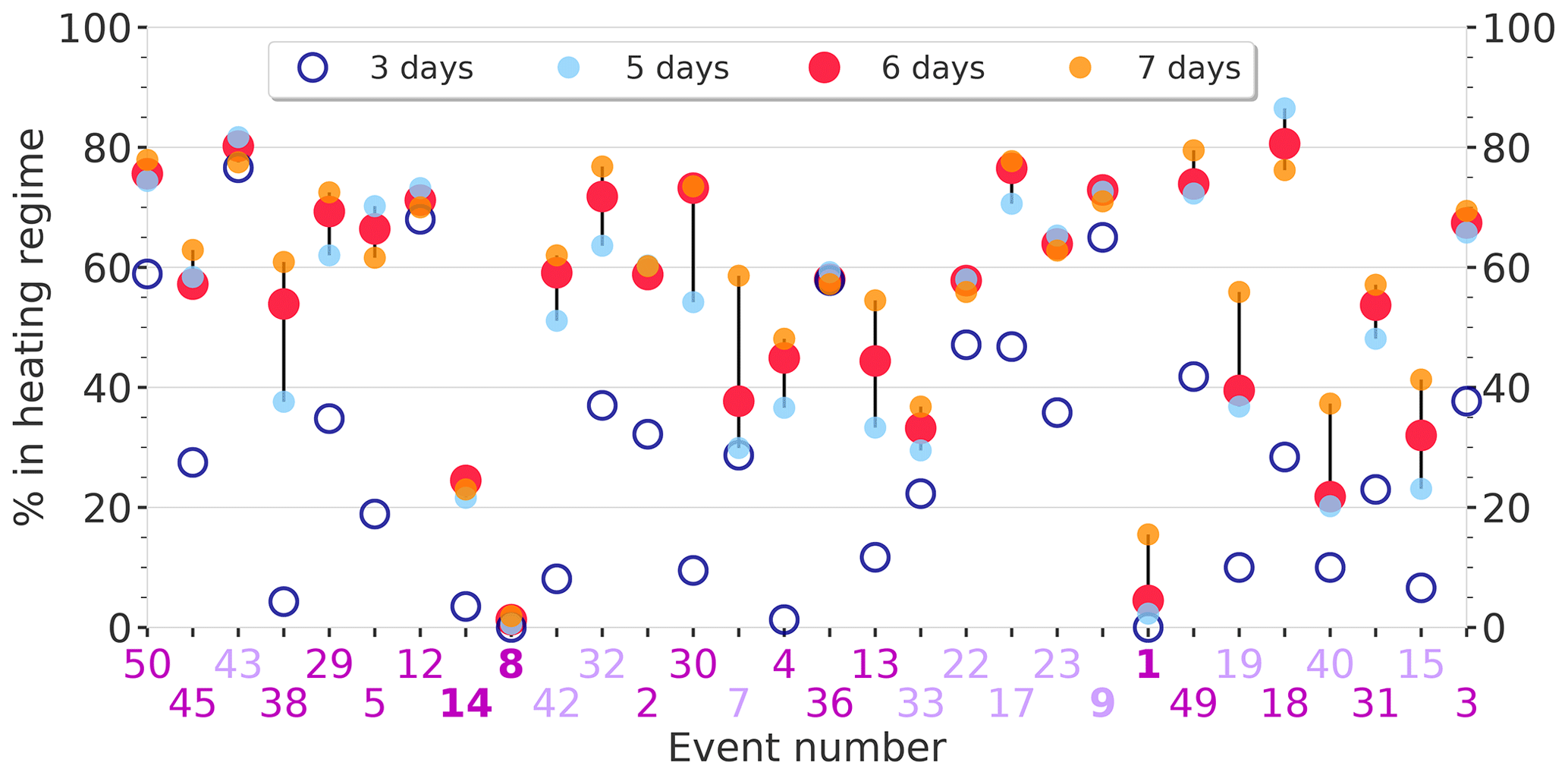
Figure 9Percentages of blocking air parcels in the heating regime shown per Ural event for back trajectories during 3 (blue), 5 (light blue), 6 (pink) and 7 (orange) days before their arrival into the blocking region. The percentages for 5 and 7 days are connected with a black vertical line. Event numbers refer to event ranking, here sorted by time, where magenta numbers refer to pure Ural events (Ural cluster), light purple to the mixed cluster and bold numbers (event 14 and 8, event 9 and 1) refer to events associated with the same block.
We turn now to the question of where geographically the diabatic heating and ascent of air parcels feeding into Ural blocks takes place. For each trajectory in the 6 d heated class, we identify the location of the peak diabatic heating rate as the point of maximum θ increase over a 6 h period between 6 and 1 d before arrival at the blocking region. To filter high-frequency noise, we first smooth the 1-hourly θ values with a 6-hourly running mean. Figure 10a presents the resulting spatial distribution of peak heating. The bulk of the trajectories (68 %) undergo peak heating in the Atlantic sector (dashed lines in the figure; see also Table 1, right), particularly in the mid-latitude central and eastern parts of the basin just west of the British Isles. This structure differs markedly from the climatological distribution presented in Steinfeld and Pfahl (2019, their Fig. 7), which shows heating concentrated in the western Atlantic off the North American coast: by focusing on Ural blocking, we are selecting a relatively infrequent subset of trajectories shifted northeastward toward the Ural sector. In addition, a substantial number of trajectories undergo heating over the eastern Mediterranean, with smaller numbers over the North American continent and the central Pacific. The relative fraction of trajectories experiencing maximum heating in the North Atlantic increases up to 86 % when applying the stricter criteria consistent with warm conveyor belts (WCBs), discussed in more detail in the Supplement (Sect. S2). The distribution shown in Fig. 10a strongly points to a connection between Ural blocking and diabatic heating in cyclones within the main North Atlantic storm track, as we explore in Sect. 6 below.
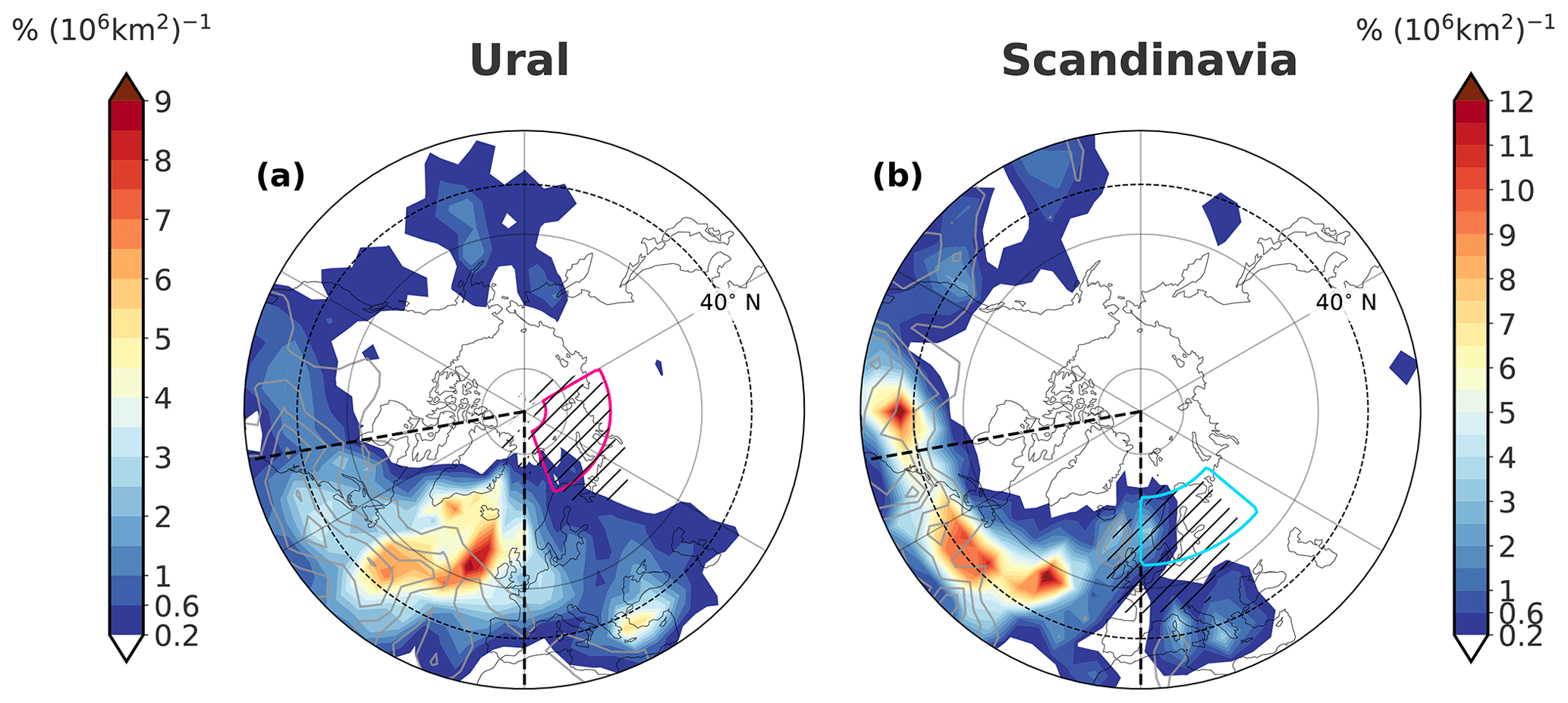
Figure 10Spatial distribution of the locations of maximum heating for the trajectories within the heating regime initialized from Ural (a) and Scandinavian (b) blocks. Shading shows the density of trajectories at the time of maximum 6-hourly heating, defined as the percentage of the total number of heated trajectories per unit area (here ). The gray contours show the locations of the trajectories 6 d prior to arrival into the blocking region (normalized area-weighted density, shown every 1 % (106 km2)−1, starting from 1 % (106 km2)−1). The magenta box in panel (a) and the cyan box in panel (b) show the Ural and Scandinavian sector, respectively, where the hatched regions indicate the main backward trajectory starting locations within the blocks (normalized area-weighted density >5 % (106 km2)−1). The main heating domain is denoted by the black dashed lines, and the black dashed circle shows the latitude line at 40∘ N.
Figure 11a shows the time evolution of trajectory density for trajectories undergoing maximum heating in the Atlantic sector (note that only 29 of the 30 events are included here, since trajectories initialized from the block associated with event 5 originate from the Pacific and are advected over Siberia). Two days before peak heating, trajectories are concentrated in the lower troposphere over the subtropical to mid-latitude western Atlantic. SLP composites at this time (shading in Fig. 11a) show a pattern corresponding to the positive phase of the North Atlantic Oscillation (NAO). This pattern is consistent with the findings of Messori et al. (2018), which show that Arctic warm extremes are preceded by a NAO+ and a northward shift of the North Atlantic jet. The positive lobe of the SLP pattern advects warm, moist subtropical air which then travels northeastward over the central Atlantic and rises rapidly, with the bulk of the ascent accomplished over the 24 h period straddling the time of peak heating (Fig. 11b). Once in the upper troposphere, air parcels are advected over the subsequent days toward the Ural sector. Similar behavior regarding the pressure evolution is observed when restricting the magnitude of ascent for the heated trajectories, though with larger pressure differences between the time of maximum heating and its near time steps (Fig. S1 in the Supplement).
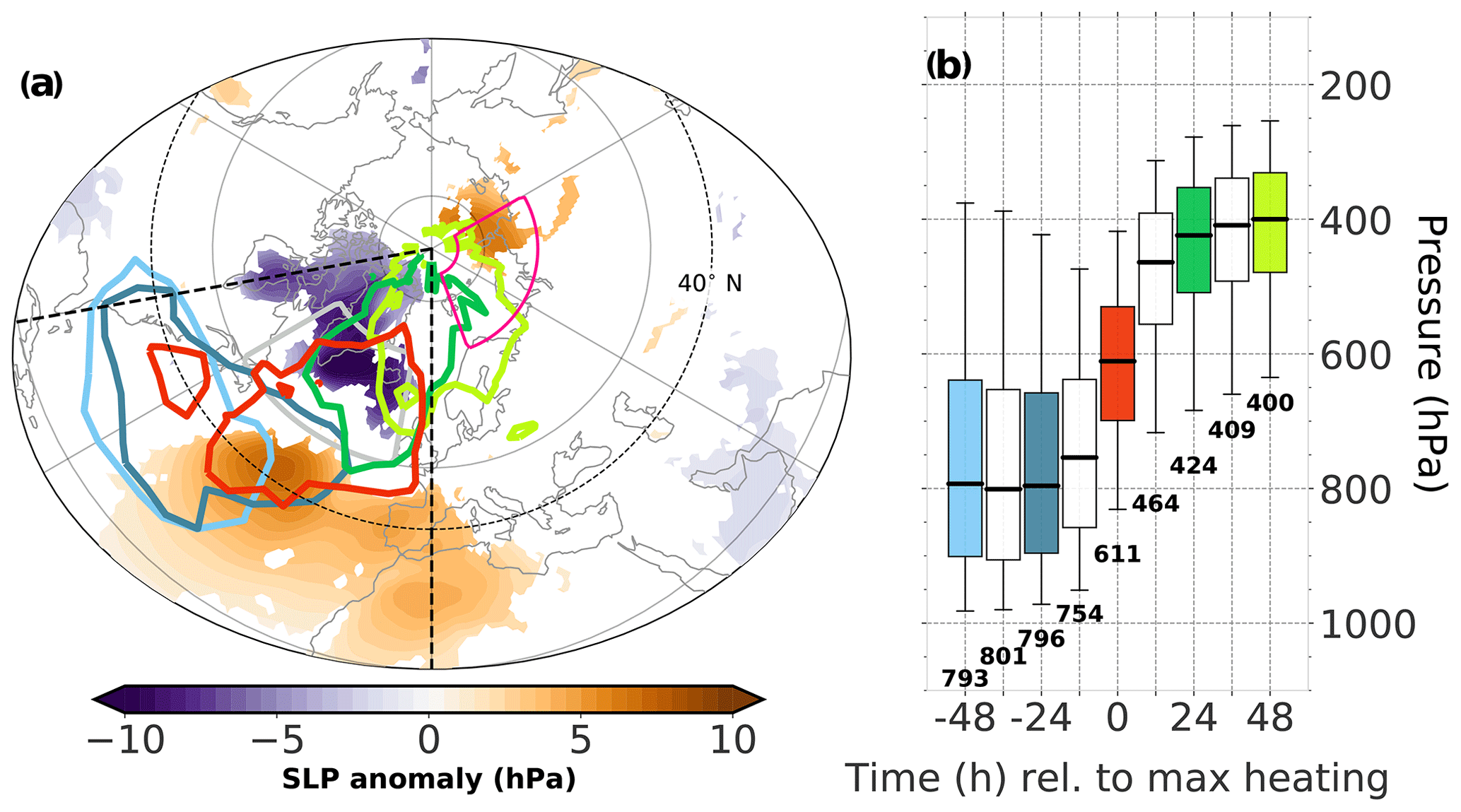
Figure 11Spatial and vertical evolution of Ural blocking trajectories belonging to the main heating domain (region denoted by the black dashed lines in panel a). (a) Significant SLP anomalies 2 d prior to the timing of the event defined peak frequency in max heating within the main heating domain (hPa, shading, significant when ≥67 % of the 30 members obtain the same sign in the anomaly as the composite mean), overlaid with density contours of trajectories at the location of max heating (red), 1 d before (turquoise), 2 d before (light blue), 1 d after (green) and 2 d after (light green), normalized by the total number of trajectories included at the corresponding time step and area weighted by each grid cell area (). Each density contour shows the 4 % (106 km2)−1 value. The magenta box denotes the Ural sector, i.e., the origin region for the blocking trajectories, and the gray box denotes the region used for analyzing cyclone activities. The dashed black circle shows the latitude band at 40∘ N. (b) Evolution of pressure along trajectories relative to the time of maximum heating within the main A domain; coloring as in panel (a). Median values per 12-hourly time slots are shown in text and as horizontal lines, boxes denote the interquartile range, and whiskers show the 5th–95th percentile range.
We have now shown that the majority of the Ural blocking trajectories undergo maximum heating and lifting in the Atlantic sector (Fig. 11), mostly in the period between 1 and 6 d prior to arrival into the blocking region (Fig. 7c). Frequency distributions over the time lag of maximum heating in the Atlantic sector, performed for individual trajectories per event, reveal that maximum heating is typically concentrated in one (70 %) or two (20 %) bursts, with the former temporally taking place either at early (longer than 3.5 d, 30 %) or late (shorter than 3.5 d, 17 %) lags or around lag −3.5 d (23 %). The remaining events experience maximum heating almost evenly within the 5 d window or lack maximum heating over the Atlantic (one event). Based on the frequency distributions, we then define for each event a time of peak heating, i.e., one lag when the majority of the heated trajectories experience maximum heating.
The maximum heating on average occurs at approximately 4 d prior to arrival in the blocking region (median lag of −3.5 d, Fig. 12b). We refer the reader to the Supplement for a discussion of the change in time of maximum heating by applying additional pressure criteria (Sect. S2 and Fig. S2 in the Supplement), where we show a shift of maximum heating to later times, closer to the blocking region, when approaching the definition of WCBs.
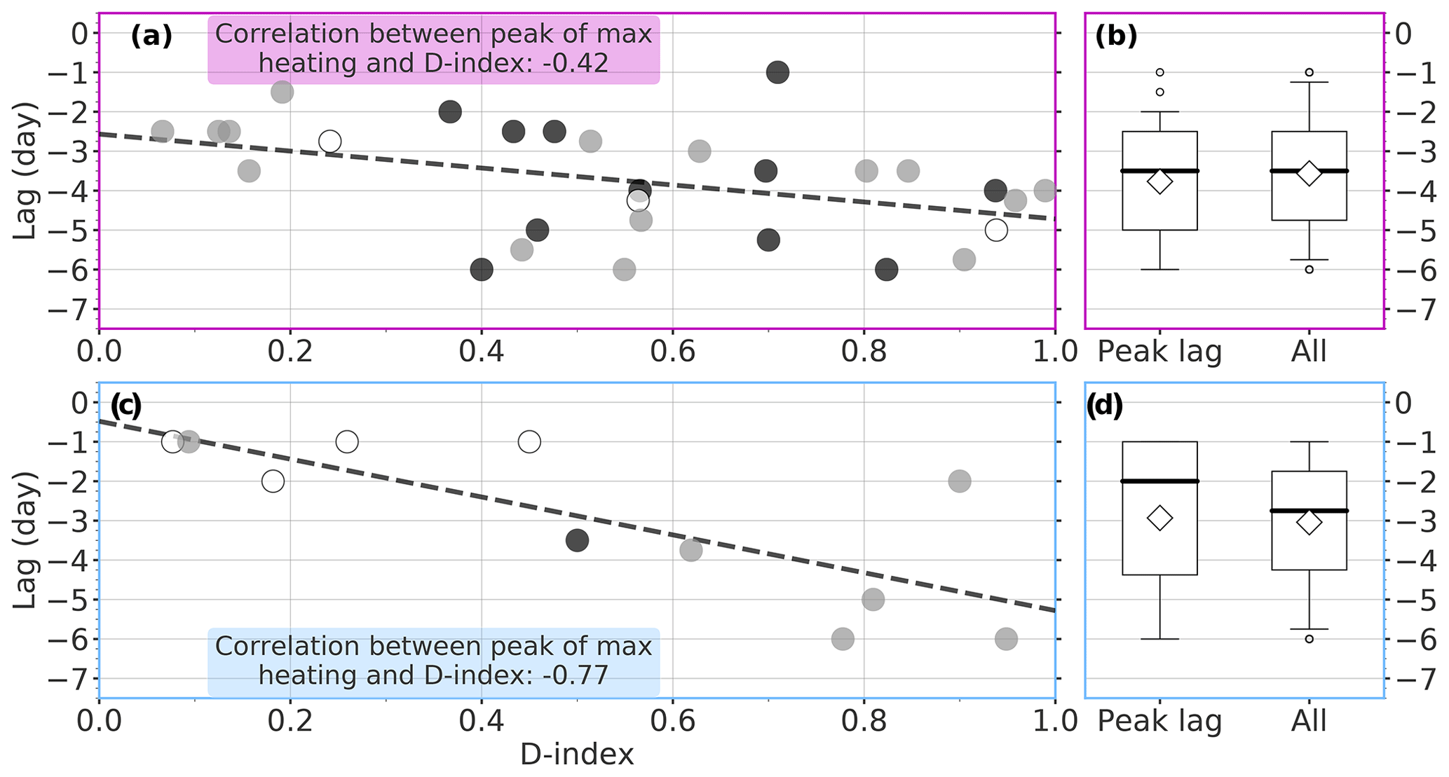
Figure 12Correlation between life stage of the Ural (first row, magenta) or Scandinavian (second row, light blue) blocks and the time lag of peak heating within the main Atlantic (A) heating domain (a, c); markers colored by the Ural (a) and Scandinavian (b) sector blocking fraction (dark-gray marker >99th percentile, white marker <90th percentile and gray in between) at trajectory starting points (see also Tables S1–S4 in the Supplement, Sect. S1). The life stage of the block at the time of trajectory initialization is given by the D index (see Eq. 1). (b, d) The distribution for the time of peak heating in the Atlantic sector (total of 29 blocks in panel b and 11 blocks in panel d) and the distribution of the time lag of peak heating defined separately for all trajectories experiencing maximum heating in the selected Atlantic sector (total of 38 825 trajectories in panel b and 11 692 in panel d) are shown in boxplots. The horizontal line denotes the median, the diamond the mean, the box the interquartile range, the whiskers the 5th–95th range and the circles the outliers.
We further find a correlation of −0.42 between the time of peak heating and the life stage of the block (D index, Eq. 1), visualized in Fig. 12a. This implies that trajectories initialized from older blocks (higher D index) generally experience peak heating in the Atlantic sector at early lags, many days prior to arrival at the block, and vice versa (as also seen for the Ural blocking trajectories presented in the case study in Sect. 3). As the sector blocking fraction partly reflects the size of the block, we observe that blocks at their mature stage (D-index values close to 0.5) usually obtain high sector fractions, as seen by the darker coloring of the markers in Fig. 11a. This is consistent with the climatology of the evolution of blocking size presented by Croci-Maspoli et al. (2007).
Lastly, when considering the time of peak heating for all heated trajectories per each Ural event, not only for those experiencing maximum heating within the Atlantic sector, we find a weaker correlation of −0.33 between the time of peak heating and the D index. This weaker dependency arises if we obtain different times of peak heating for an event for these two cases, especially when only a minority of the air parcels experience maximum heating in the Atlantic sector. The event-wise defined peak lags for both cases discussed above, as well as the relative fractions of heated trajectories being heated over the Atlantic and the D index related to each block, are listed in the Supplement (Sect. S1) in Tables S1–S4.
5.2 Scandinavian blocking
This section examines the dynamics behind Scandinavian blocking events, following the same approach as for Ural events in the previous section. Back trajectories are initialized from blocks observed over the Scandinavian sector (Table 1; see also light-blue sector in Fig. 5d). In Fig. 6a, markers overlaid with a small black dot denote the 10 events included here, namely six pure Scandinavian events and an additional four events from the mixed Ural–Scandinavian cluster which show an isolated blocking region over Scandinavia. To enable comparison with the Ural case and analyze blocking trajectories initialized within lags −3 to −1 d relative to trajectory starting points, events where the block decays more than 3 d prior to the peak warm anomaly are excluded. One of the pure Scandinavian events (event 24) features two separate blocks, which are treated separately here. This leaves us with 10 Scandinavian events consisting of 11 blocks for the Lagrangian analysis performed in this section. One event obtains scattered blocking regions, to which a geographical mask is applied in order to retain only the region of the block located over Scandinavia (see footnote in Table S3 in the Supplement, Sect. S1). We compute a total of 32 255 trajectories initialized on the day of maximum Scandinavian blocking fraction: 3 d prior to the Arctic warm event in five cases and 1 d prior in six cases.
The frequency distributions of Δθ for different trajectory lengths (Fig. 7b) resemble the distributions obtained for the Ural events, with a bimodal structure and increased heating and cooling for longer trajectories. However, the fraction of heated trajectories (inset panel in Fig. 7b) increases more rapidly than in the Ural case, reaching 41 % already at 3 d for Scandinavian events compared to 32 % for the Ural case. This rapid increase saturates after 5 d; by 6 d, the heating fraction of 58 % (18 595 heated trajectories) is comparable to Ural case. The case-to-case variability of the computed heating fractions at 6 d is much smaller for the Scandinavian than for the Ural events: 10 of 11 Scandinavian blocks obtain fractions over 40 %, with a minimum fraction of 36 % (see Table S3 in the Supplement, Sect. S1). As a result, the average over the per-event fractions at 6 d is actually 60 %, which is somewhat higher than the respective value for the Ural events. Thus, diabatic heating has an important role also for Scandinavian blocking events.
At 6 d before arrival in the blocking region, about 75 % of trajectories in the heating regime are in the lower troposphere, at pressures >500 hPa (Fig. 7d). As for the Ural cases, the median trajectory is close to 700 hPa but with a higher θ of 308 K. From here, the air parcels warm and rise into the upper troposphere, obtaining a median heating of 10 K for 6 d trajectories (Fig. 8b). The ascent rate within 2 d and the change in specific humidity along the heated trajectories are slightly smaller in magnitude compared to the Ural ones, obtaining median values of around 300 hPa (Fig. 8f) and a drying of around 3 g kg−1 (Fig. 8j), respectively. On the other hand, trajectories in the non-heating regime are almost totally in the upper troposphere on day −6 (Fig. 7f), obtaining similar cooling rates as for the Ural ones (Fig. 8b) and an insignificant change in the specific humidity (Fig. 8j).
Turning to the question of where the diabatic heating of air parcels feeding into Scandinavian blocks takes place, the spatial distribution of the peak heating location (Fig. 10b) shows that it is again mostly in the Atlantic sector, but with marked displacement toward the southwest, in closer correspondence with the climatological distribution (Steinfeld and Pfahl, 2019). In addition, a considerable number of trajectories undergo maximum heating over eastern North America and smaller numbers over the eastern Mediterranean and the eastern Pacific. Nonetheless, as seen for the Ural events, the distribution shown in Fig. 10b similarly suggests a connection between Scandinavian blocking and diabatic heating in mid-latitude Atlantic cyclones.
As for the Ural events, the maximum heating of Scandinavian blocking trajectories experiencing maximum heating in the Atlantic sector temporally takes place in one (91 %) or two (9 %) bursts, with the former being clearly larger than for the Ural ones. Furthermore, almost half of the events in the former experience peak heating at later lags (shorter than 3 d, 46 %), whereas earlier lags (longer than 3 d) or heating around day −3, favored by the Ural events, here are less preferred (18 % and 27 %, respectively). Most of the heating takes place at later lags, closer to the blocking region, with a median lag of about −2 d (Fig. 12d), which is clearly smaller compared to the median lag of −3.5 d obtained for the Ural events (Fig. 12b). The bulk of the temporal distribution for peak heating defined separately for all individual trajectories experiencing maximum heating in the Atlantic sector is shifted to slightly earlier lags, though with a median lag of −3 d, as seen in Fig. 12d, right. However, Scandinavian blocking trajectories tend to experience maximum heating in the Atlantic sector generally at later lags compared to the Ural events, which is consistent with the fact that about 40 % of the Scandinavian blocking air parcels experience heating already in the first 3 d after initialization (Fig. 7b). The negative correlation we found between the per-event time of peak heating over the Atlantic and the life stage of the Ural blocks at the time of trajectory initialization becomes even more pronounced for Scandinavian blocks, showing a strong negative correlation of 0.8 as seen in Fig. 12c. Three events at the time of trajectory initialization obtain blocking sector fractions below the 90th percentile, but as expected, these blocks are at their onset or early mature stage (D index below 0.5). The individual peak lags and D-index values for Scandinavian blocks are listed in Tables S3 and S4 in the Supplement (Sect. S1).
The previous section showed that most diabatically heated trajectories associated with both Ural and Scandinavian blocks undergo heating and lifting in the time period between −6 and −1 d relative to blocking starting points. Figure 13 shows the tracks of all cyclones present during this 5 d interval for all Ural (a) and Scandinavian (b) events. In the North Atlantic, the tracks are characterized by large-scale cyclonic motion around Greenland, consistent with the large-scale dipole in the SLP anomaly composite shown in the same figure. The tracks are particularly concentrated in the region marked by the yellow box (50–70∘ N, 10–60∘ W) positioned immediately to the northwest of the area where maximum diabatic heating is concentrated (Fig. 10), consistent with the idea that diabatic heating occurs predominantly in the warm sectors to the southeast of the cyclone centers. Each event has at least two (up to seven) cyclones that reside in the yellow box at some time within the relevant 5 d period, and 90 % of all these events obtain at least one (up to three) cyclones located within the box at the time of peak heating. For the remaining four events, the yellow dot is located just west or north of the box, and the majority of the red-colored cyclones either experience genesis shortly after the time of peak heating or undergo lysis just before it. Nevertheless, the majority of the yellow markers reside within or close to the yellow box, confirming the importance of cyclones for the diabatic heating experienced by the blocking trajectories.
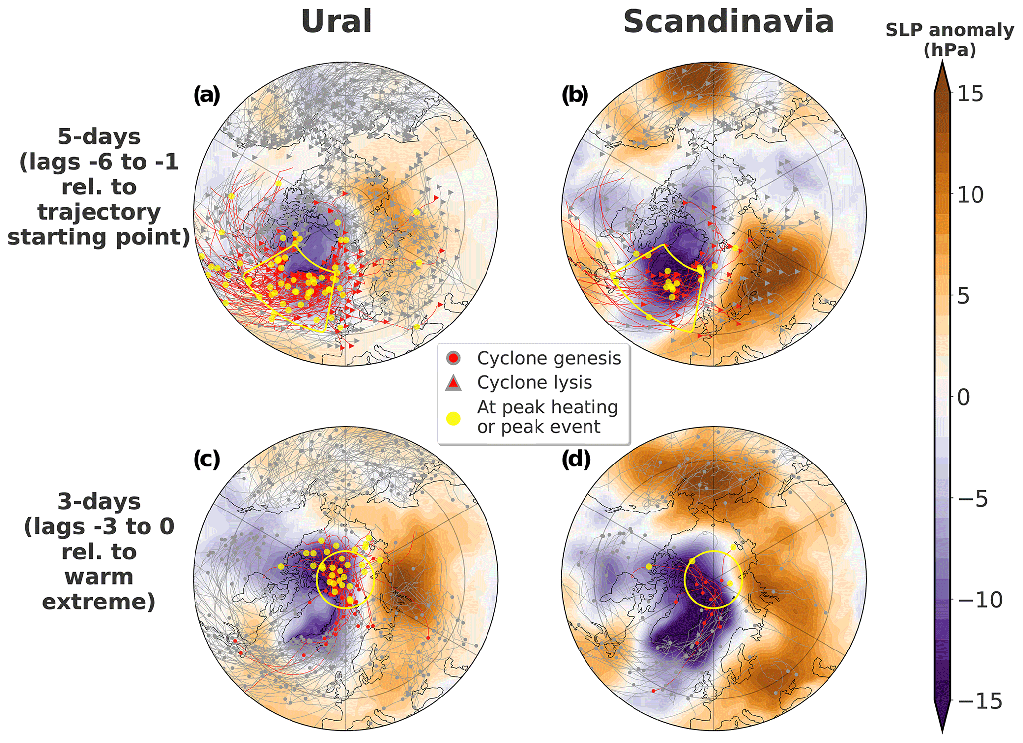
Figure 13Cyclone track distribution around warm extremes related to Ural (left column) or Scandinavian (right column) blocks. (a, b) Cyclones observed within lags −1 to −6 d relative to trajectory initialization (blocking region), shown for 30 Ural (a) and 10 Scandinavian (b) events, respectively. Tracks are colored red if the selected cyclone is both in temporal and spatial correspondence with the considered time period in the yellow sector (C; 50–70∘ N, 10–60∘ W). If there is only a temporal match, the cyclones are colored gray. Shading shows the SLP anomaly composite over these events at the case-defined peak of maximum heating within the main heating domain for blocking trajectories (for 29 Ural and 10 Scandinavian events in panels (a) and (b), respectively; see also Tables S2 and S4 in the Supplement, Sect. S1). Yellow circles show the location of the red-colored cyclones at this peak of maximum heating. Red or gray solid triangles show the lysis of cyclones that cross or stay outside the chosen sector, respectively. (c, d) Same as in panels (a) and (b) but shown for cyclones observed up to 3 d prior to the peak of each Ural (c) or Scandinavian (d) event, respectively, where the red coloring refers to cyclones that reside in the high Arctic (≥80∘ N, yellow latitude band at 80∘ N) within the time period considered. The SLP anomaly composite field and yellow circles for the red-colored cyclones are shown at the time of each warm event. Red and gray solid circles denote the genesis of cyclones that cross or stay outside the chosen sector, respectively.
For the 30 Ural cases, an average of five cyclone tracks per event cross the yellow box in Fig. 13a during the relevant 5 d window preceding blocking (involving values between a minimum of two and a maximum of seven crossings in individual cases). To compare with climatology, we select 30 random winter pentads, compute the mean number of crossings per pentad and repeat 500 times. This procedure yields a median of only four cyclone crossings per pentad (Fig. 14) and shows that the 30 Ural cases constitute a rare sample with exceptionally high mean cyclone activity, which is well above the 99th percentile of the climatological distribution. The 10 Scandinavian cases, on the other hand, show an average of only four cyclone crossings per event (interval 3–6); comparison with climatology using random sampling of 10 pentads shows that this average lies within the interquartile range and cannot be considered exceptional. These results indicate that serial cyclone clustering (Pinto et al., 2013) can be important for generating Arctic warm events, at least in those cases associated with Ural blocking.
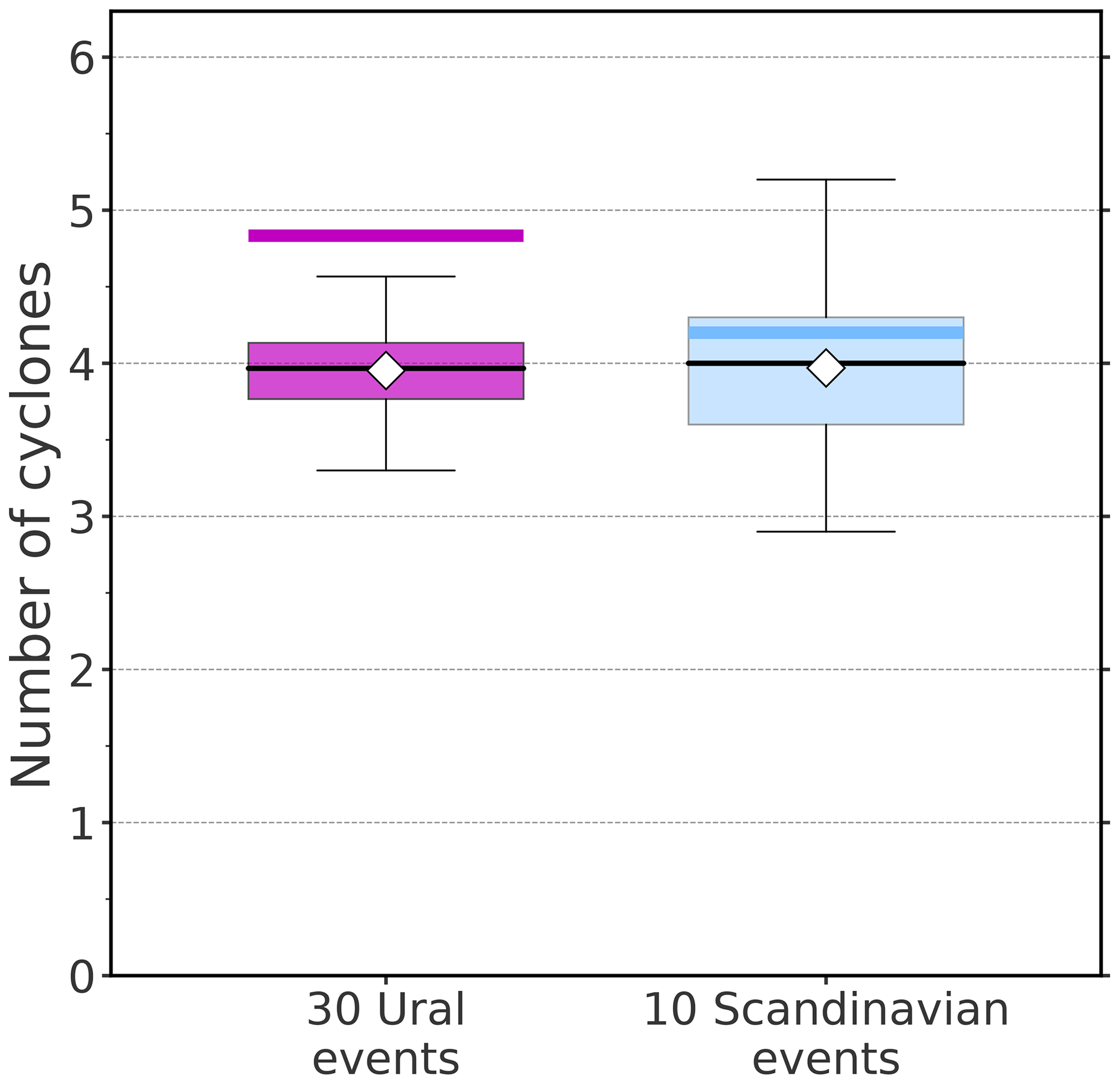
Figure 14Cyclone climatology presented as the average cyclone frequency observed in the chosen sector (C, yellow sector in Fig. 13a and b; 50–70∘ N, 60–10∘ W) northwest of the main heating region during a 5 d window (lags −1 to −6 d relative to trajectory initialization within the block) for 30 Ural (magenta) and 10 Scandinavian (light blue) events, computed using Monte Carlo resampling of 30 or 10 arbitrary events within the analysis period with 500 repetitions, respectively. The black horizontal line denotes the median, mean is shown with diamonds, the box refers to the IQR and the whiskers denote the 1st–99th percentile range of the distribution. The magenta and light-blue horizontal lines at each boxplot denote the cyclone frequency for the 5 d window averaged over the 30 or 10 chosen Ural and Scandinavian events, respectively.
Returning to Fig. 13, we note that with the exception of a few cyclones, almost all of the red tracks in the figure experience lysis either within the yellow box or immediately to the north, northeast and west of the box; only a handful continue northward to enter the Arctic. To further quantify whether the majority of Arctic cyclones at the time of peak event undergo genesis in high latitudes, we select cyclone tracks present during a 3 d period leading up to each of the Ural (Fig. 13c) or Scandinavian (Fig. 13d) warm events, respectively. Here, cyclone tracks observed within the polar cap (≥80∘ N, yellow circle) during the selected time window are colored red, and the genesis points of these cyclones are denoted by a red solid circle. Two Ural and three Scandinavian events lack cyclones fulfilling the aforementioned criteria. For the remaining events, we observe that the majority of the red dots reside in the high latitudes, where the 70∘ N latitude band encompasses 87 % and 83 % and the polar cap encloses 67 % and 42 % of all genesis locations for the 54 and 12 red colored cyclones related to Ural (Fig. 13c) and Scandinavian (Fig. 13d) events, respectively. Even though Scandinavian events in general obtain less Arctic cyclones with local genesis around the peak of the event compared to the Ural events, our results presented here support the results of Messori et al. (2018) showing that cyclones present in the high Arctic around the time of peak event are mainly locally generated within the polar cap or in the close vicinity of it. Only a few of the red-colored cyclone tracks undergo genesis in the mid-latitudes (see, e.g., the two red dots at 50∘ N in Fig. 13c). In fact, these two cyclones are related to event 9, of which one is shown to be responsible for the lifting of the Ural blocking trajectories in the Atlantic sector, as discussed in the case study in Sect. 3.2. Another interesting difference between these two cases is the location of the selected cyclones at the peak of each event (yellow markers on red tracks), where 60 % of the 30 red cyclones existing at the peak of Ural events (Fig. 13c) reside within the polar cap, whereas already half of the four red cyclones prevailing at the peak of Scandinavian events have exited the polar cap (Fig. 13d).
As seen by the SLP anomaly composite (shading in Fig. 13c and d) representing the peak of each warm event, the region of negative SLP anomalies in the northwestern Atlantic is displaced northwards, now reaching all the way into the Arctic. On the other hand, the region of positive SLP anomalies over the Urals in Fig. 13c becomes even more pronounced at the peak of the warm events. For the Scandinavian events, there are two distinct centers of positive SLP anomalies – one over Scandinavia and one over the Urals, with the latter due to the four events from the mixed cluster.
Previous studies show that Ural blocking enhances Arctic warming and sea-ice loss especially over the Barents–Kara seas (Luo et al., 2016b, 2017, 2019; Gong and Luo, 2017) and that Ural blocks are able to produce stronger sea-ice decline compared to Scandinavian blocking (Luo et al., 2019). This is in agreement with our findings, where 37 of the top-50 wintertime high-Arctic warm extreme events are attributed to blocking over the Urals, Scandinavia or over both regions simultaneously, with a majority of events featuring a strong Ural block preceding peak warming in the high Arctic. The majority of the residual events show a weaker ridge over the Urals, which is consistent with the study from Kim et al. (2021), showing that 22 % of the WACE patterns are in fact driven by weaker anticyclonic anomalies over the Urals rather than a stronger blocking high.
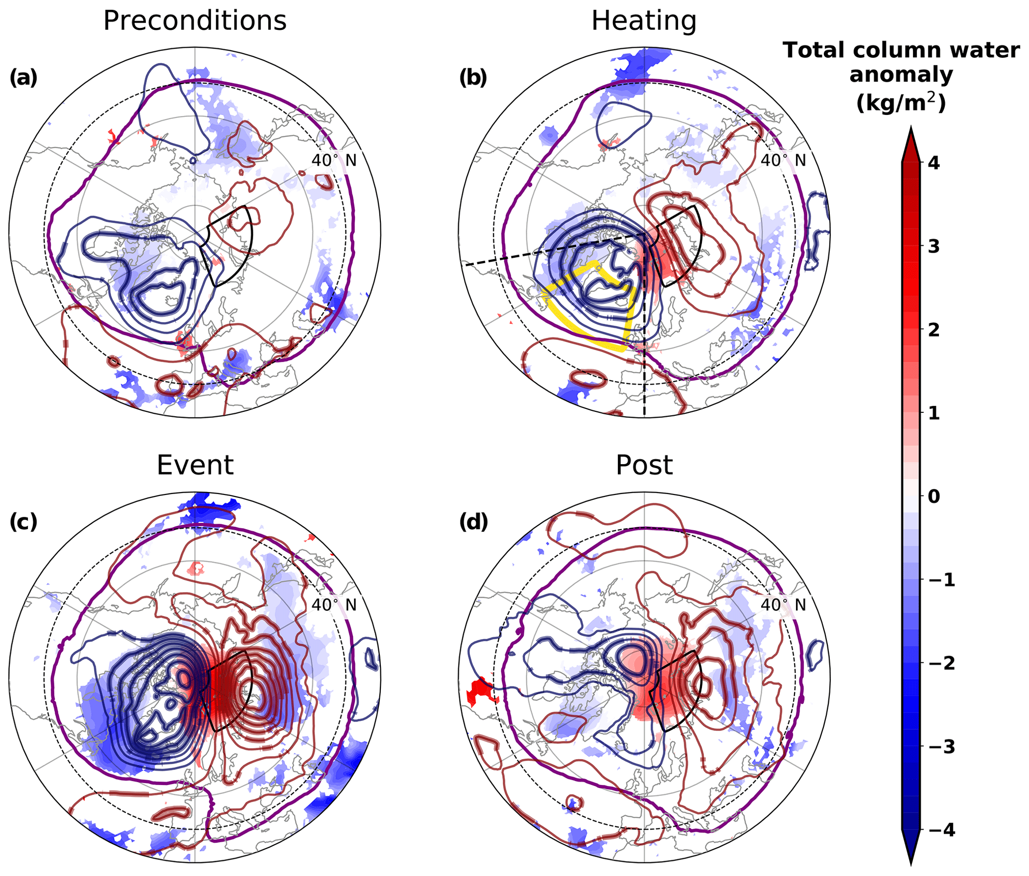
Figure 15Chain of processes related to Ural warm events as time and event composite during four identified time periods: at preconditions (days −9 to −6 relative to trajectory initialization, 3 d per event) (a), at heating (−6 to −1 d with respect to trajectory initialization, 5 d per event) (b), in the close vicinity of the warm events (days between lag −1 d relative to trajectory initialization until the peak of warm event, 2–4 d per event) (c) and at post conditions (up to 3 d after each warm event, 3 d per event) (d). Significant total column water anomalies shown in shading (kg m−2, significant when >67 % of the 30 members obtain the same sign in the anomaly as the composite mean), overlaid with SLP anomalies (hPa, every 5 hPa, significant in bold contours, red for positive, blue for negative anomalies, zero anomaly contour not shown) and potential temperature on the 2 pvu surface (purple solid isoline for 310 K). The black dashed region in panel (b) denotes the main heating region, the yellow sector in panel (b) the cyclone region and the dashed black circle shows the latitude band at 40∘ N.
Next we discuss the sequence of dynamical processes, based on the 30 warm events associated with Ural blocking, leading to these warm extremes in the high-Arctic (Fig. 15).
-
The first stage, “preconditions” (Fig. 15a), comprises days 9 to 6 prior to peak Ural blocking, i.e., the time before the majority of the trajectories experience diabatic heating. This period is characterized by a subtropical high-SLP anomaly and significant negative SLP anomalies over Greenland – a pattern resembling the positive phase of NAO (NAO+). The circulation pattern promotes eastward/northeastward advection of warm and moist air towards the central Atlantic. Already at this stage, some events exhibit positive SLP anomalies over the Urals.
-
The second stage, “heating”, comprises the 5 d period (6 to 1 d preceding the peak in Ural blocking) when most trajectories experience diabatic heating (Fig. 15b). The NAO+ phase continues, with deeper negative SLP anomalies found over Greenland (Fig. 15b), and the positive SLP anomalies over north Siberia strengthen, forming a dipole over the Nordic Seas conducive to advection of warm and moist air into the high Arctic.
We find that the majority (68 %) of the 6 d heated Ural blocking trajectories experience lifting and maximum diabatic heating in the mid-latitude North Atlantic during this 5 d period. The spatial distribution of maximum heating (Fig. 10a) differs markedly from the climatological distribution presented in Steinfeld and Pfahl (2019) and regions favored by ascending WCBs, as shown by Madonna et al. (2014). For the warm events preceded by Scandinavian blocks (Fig. 10b), on the other hand, the distribution better resembles those in the studies cited above.
Additionally, this 5 d period is characterized by anomalously high cyclone activity within a region (yellow box in Fig. 15b), consistent with the region of negative SLP anomalies, located northwest of the region favored by maximum heating for blocking trajectories. This is consistent with the NAO+, characterized by a higher activity of intense wintertime North Atlantic cyclones (Pinto et al., 2009). The combination of NAO+ pressure pattern and Ural blocking ensures a pathway for moisture transport from North Atlantic into the Arctic and thus promotes Arctic warming and sea-ice decline (Luo et al., 2017, 2019; Papritz and Dunn-Sigouin, 2020; Fearon et al., 2020).
-
The “event” stage (Fig. 15c) coincides with the 1–3 d time window between the peak in Ural blocking fraction and the peak of the warm event. The lag between the peak Ural blocking and peak Arctic warming found here is in line with a lag of 4 d found between Ural blocks and observed warming and sea-ice loss over the Barents–Kara seas (Gong and Luo, 2017). The formation or strengthening of Ural blocking at this stage, subsequent to the NAO+ event noted in prior stages, is consistent with previous work showing a development of Ural blocks 4–7 d after NAO+ (Luo et al., 2016a). The combined effect of a decaying NAO+ pattern and the growing block over the Ural Mountains is to create an SLP anomaly dipole (Fig. 15c) enabling penetration of heat and moisture into the polar cap, leading to Arctic warming (Fearon et al., 2020; Papritz and Dunn-Sigouin, 2020). These results support the importance of Ural blocking or similar circulation anomalies over the Urals in promoting horizontal temperature advection (Kim et al., 2021) or enhanced moisture flux convergence (Gong and Luo, 2017) in the periphery of the blocks, thus giving rise to warming in the high-Arctic, especially via the increased downward longwave radiation in the Arctic. This anomalous moisture transport is also seen in Fig. 15c, which shows significant positive moisture anomalies over the Arctic Ocean.
-
The “post” stage (Fig. 15d) is represented by a composite over 3 d after the warm event. Here, the upper-level forcing is diminishing and the dipole in the SLP pattern clearly weakens, concomitant with weaker moisture anomalies over the central Arctic.
As noted by Luo et al. (2016a), the formation and strengthening of the Ural blocking anomaly subsequent to the NAO+ may be the result of wave activity propagation from the decaying NAO+ towards the Ural Mountains. Furthermore, the high cyclone activity prior to peak Ural blocking can contribute to the block development by the remote baroclinic source, thus feeding wave activity towards the block (Wang et al., 2021), as well as being influenced by the background flow. Our findings do not contradict the important role of adiabatic processes but rather provide additional insight into the amplification mechanisms of Ural blocks in the light of moist-dynamic processes, as also shown by recent studies (e.g., Pfahl et al., 2015; Steinfeld and Pfahl, 2019; Steinfeld et al., 2020). Specifically, we find that the diabatic outflow downstream of cyclones associated with their WCBs has a crucial role on the upper-level circulation by injecting low-PV air in the upper troposphere and thus helps maintain and strengthen the upper-level block; around 60 % of the air parcels in Ural blocks are subject to diabatic heating over the 6 d period prior to peak blocking. These results hint at a self-amplifying mechanism behind Ural blocks: they are potentially initiated by adiabatic wave propagation and, once established, promote further advection of low-PV diabatically processed air into the block as it is produced in the ascending branches of North Atlantic cyclones. Further study of this self-amplifying mechanism could be an interesting avenue for future work.
The mechanisms responsible for the demise of the Ural blocks is not further analyzed in this study. However, we find air masses recirculating within the upper-level block for several days after diabatic heating and occasionally a high event-wise contribution of non-heated trajectories, both subject to diabatic cooling of around 8 K over 6 d (see Fig. 7a), most likely caused by longwave radiative cooling. The low fraction of heated trajectories is particular for blocks in their decaying stage, consistent with previous studies (Pfahl et al., 2015; Steinfeld and Pfahl, 2019; Steinfeld et al., 2020). Following Wang et al. (2021), local diabatic cooling in the decaying stage of the blocking life cycle may have a dampening effect through radiative decay of PV anomalies in the upper-level block, especially concurrently with weakening dry barotropic wave advection and baroclinic wave propagation.
Given the key role of blocking and its interaction with mid-latitude cyclones – cyclones as a potential amplifier of the blocks that further guide cyclones northwards – as a driver for the top-50 Arctic wintertime warm extremes that we find here, another interesting question that arises is whether this is also a common feature in other, less extreme warm events in the high Arctic. Starting from a blocking perspective and applying the methods used in this study could help enhance our understanding of the processes responsible for Arctic warming. A further promising avenue for further investigation would be to study events based on anomalies in the surface energy budget rather than in temperature, as the former directly affects sea-ice development and could allow for deeper insights into the dynamical processes responsible for sea-ice decline in the Arctic.
We have investigated the dynamics behind the 50 most extreme wintertime high-Arctic warm anomalies, focusing on the importance of Ural and Scandinavian blocking preceding the warm extremes. Furthermore, the dynamical processes responsible for the emergence of these events were assessed, focusing mainly on the contribution of diabatic heating in mid-latitude cyclones to the formation and amplification of the blocks. We answer the questions posed in the introduction as follows.
-
What is the role of blocking in driving the extreme warm events?
Blocking plays a central role for the majority of the top-50 warm events: composites of vertically averaged upper-tropospheric potential vorticity anomalies over the 50 events show a prominent negative anomaly over the Ural and Scandinavian sectors. The surface expression of this pattern is a SLP anomaly dipole between a high over Siberia and a low over Greenland, promoting warm and moist air advection into the high Arctic.
-
Are there regional differences in the circulation patterns?
We find regional differences in the circulation patterns among the different warm extremes: 30 events are associated with Ural blocking – 18 of which have a block only over the Urals and 12 obtaining blocking over both Scandinavia and the Urals – where the peak blocking is preceded by a NAO+ pattern. Furthermore, seven events were found to be preceded by Scandinavian blocking and two by strong blocking over the Pacific, whereas 11 events – resembling the structure of Ural events but with a weaker amplitude – were not associated with any block in the three favored blocking regions.
-
What is the importance of diabatic processes in driving the blocks?
By tracing low-PV air masses 6 d backwards from Ural blocks preceding high-Arctic warm events, we have found that around half (59 %) of the air parcels experience lifting (median ascent of 363 hPa within 2 d) and diabatic heating (median heating of 11 K), which emphasizes the importance of diabatically heated trajectories for Ural blocks. For Scandinavian blocks associated with the warm extremes, located mainly southwest of the Ural blocks, the partitioning into heated (58 %) and non-heated trajectories reveals similar percentages as for Ural blocks when considering 6 d. However, almost half of the air parcels making up the negative VAPV anomalies of Scandinavian blocks experience heating already within the 3 d journey into the blocking region, which is a remarkably higher contribution compared to a third when considering Ural blocking trajectories. The strongest heating is found over a region in the North Atlantic, temporally taking place at a median day of 3.5 and 2.75 prior to arrival into the Ural and Scandinavian blocks, respectively.
Furthermore, we find that the time of peak heating within the North Atlantic region, defined per each Ural and Scandinavian event, and the life stage of the blocks are negatively correlated, indicating that younger blocks experience maximum heating preferably at later times, closer to the blocking region and vice versa.
-
How do cyclones and blocks interact during the events?
We find a strong interaction between mid-latitude cyclones and Eurasian blocks as a driver of wintertime Arctic warm extremes: an exceptionally high mid-latitude cyclone activity – coinciding both spatially and temporally with the time window of maximum heating for blocking trajectories in the North Atlantic – highlights the importance of latent heat release in cloud-diabatic processes ahead of strong surface cyclones in providing low-PV air into upper-level block, thus bringing out its crucial role in enhancing and amplifying the high-latitude blocks in addition to other dry-adiabatic processes. On the other hand, these cyclones are also guided polewards by the block and the anticyclonic circulation over Eurasia, further promoting northward transport of heat and moisture and thus helping generate the Arctic warm extremes. These mid-latitude cyclones mostly decay before entering the high Arctic, whereas around the time of each warm event, a peak in locally generated polar cyclone activity is observed. For Scandinavian events, on the other hand, the cyclone activity is not as exceptional.
This study deepens the understanding of the underlying processes driving the warming seen in the high Arctic, emphasizing the importance of atmospheric blocks and their tight interaction with mid-latitude cyclones – as amplifiers of the block or being guided by the block – as well as the combined effect of the prevailing circulation patterns on the appearance of high-Arctic extreme warm events. It also highlights processes that need to be well captured in models to be able to represent the Arctic wintertime climate.
Code for the analysis is available upon request.
ERA-Interim data can be obtained from ECMWF via https://www.ecmwf.int/en/forecasts/datasets/archive-datasets/reanalysis-datasets/era-interim (Dee et al., 2011).
The supplement related to this article is available online at: https://doi.org/10.5194/wcd-3-21-2022-supplement.
SM, GS and RC developed research ideas and designed the study. LP helped with the trajectory calculations. The analysis was performed by SM while continuously discussing results with RC and GS. SM wrote the initial draft of the manuscript, and all authors contributed with feedback and reviews to the sections. The final draft was edited by all authors, providing suggestions and improvements for the final version.
At least one of the (co-)authors is a member of the editorial board of Weather and Climate Dynamics. The peer-review process was guided by an independent editor, and the authors also have no other competing interests to declare.
Publisher's note: Copernicus Publications remains neutral with regard to jurisdictional claims in published maps and institutional affiliations.
We thank Erica Madonna (University of Bergen) for providing us with the cyclone tracks and ETH Zürich, especially Michael Sprenger, for all the technical support and help in the setup for the LAGRANTO tool as well as for their inspiring and helpful advice. We are also grateful for helpful discussions with Timo Vihma and Tiina Nygård (FMI). The data analysis and visualization in this study was done using Python.
This research has been supported by the Knut och Alice Wallenbergs Stiftelse (grant no. 2016-0024).
This paper was edited by Yang Zhang and reviewed by two anonymous referees.
Årthun, M., Eldevik, T. R., and Eldevik, T.: On Anomalous Ocean Heat Transport toward the Arctic and Associated Climate Predictability, J. Climate, 29, 689–704, https://doi.org/10.1175/JCLI-D-15-0448.1, 2016. a
Baggett, C., Lee, S., and Feldstein, S.: An investigation of the presence of atmospheric rivers over the North Pacific during planetary-scale wave life cycles and their role in Arctic warming, J. Atmos. Sci., 73, 4329–4347, https://doi.org/10.1175/JAS-D-16-0033.1, 2016. a
Binder, H., Boettcher, M., Grams, C. M., Joos, H., Pfahl, S., and Wernli, H.: Exceptional air mass transport and dynamical drivers of an extreme wintertime Arctic warm event, Geophys. Res. Lett., 44, 12028–12036, https://doi.org/10.1002/2017GL075841, 2017. a, b, c
Boisvert, L. N., Petty, A. A., and Stroeve, J. C.: The impact of the extreme winter 2015/16 Arctic cyclone on the Barents–Kara Seas, Mon. Weather Rev., 144, 4279–4287, https://doi.org/10.1175/MWR-D-16-0234.1, 2016. a, b
Cohen, J., Screen, J. A., Furtado, J. C., Barlow, M., Whittleston, D., Coumou, D., Francis, J., Dethloff, K., Entekhabi, D., Overland, J., and Jones, J.: Recent Arctic amplification and extreme mid-latitude weather, Nat. Geosci., 7, 627–637, https://doi.org/10.1038/ngeo2234, 2014. a, b
Colucci, S. J.: Explosive cyclogenesis and large-scale circulation changes: Implications for atmospheric blocking, J. Atmos. Sci., 42, 2701–2717, https://doi.org/10.1175/1520-0469(1985)042<2701:ECALSC>2.0.CO;2, 1985. a
Croci-Maspoli, M. and Davies, H. C.: Key dynamical features of the 2005/06 European winter, Mon. Weather Rev., 137, 664–678, https://doi.org/10.1175/2008MWR2533.1, 2009. a, b, c, d
Croci-Maspoli, M., Schwierz, C., and Davies, H.: A multifaceted climatology of atmospheric blocking and its recent linear trend, J. Climate, 20, 633–649, https://doi.org/10.1175/JCLI4029.1, 2007. a, b, c
Cullather, R. I., Lim, Y.-K., Boisvert, L. N., Brucker, L., Lee, J. N., and Nowicki, S. M. J.: Analysis of the warmest Arctic winter, 2015–2016, Geophys. Res. Lett., 43, 10808–10816, https://doi.org/10.1002/2016GL071228, 2016. a
Dee, D. P., Uppala, S. M., Simmons, A., et al.: The ERA-Interim reanalysis: Configuration and performance of the data assimilation system, Q. J. Roy. Meteor. Soc., 137, 553–597, https://doi.org/10.1002/qj.828, 2011 (data available at: https://www.ecmwf.int/en/forecasts/datasets/archive-datasets/reanalysis-datasets/era-interim, last access: 23 March 2017). a, b
Ding, Q., Schweiger, A., L'Heureux, M., Battisti, D. S., Po-Chedley, S., Johnson, N. C., Blanchard-Wrigglesworth, E., Harnos, K., Zhang, Q., Eastman, R., and Steig, E. J.: Influence of high-latitude atmospheric circulation changes on summertime Arctic sea ice, Nat. Clim. Change, 7, 289–296, https://doi.org/10.1038/nclimate3241, 2017. a, b
Doyle, J., Lesins, G., Thackray, C., Perro, C., Nott, G., Duck, T., Damoah, R., and Drummond, J.: Water vapor intrusions into the High Arctic during winter, Geophys. Res. Lett., 38, L12806, https://doi.org/10.1029/2011GL047493, 2011. a
Fearon, M. G., Doyle, J. D., Ryglicki, D. R., Finocchio, P. M., and Sprenger, M.: The Role of Cyclones in Moisture Transport into the Arctic, Geophys. Res. Lett., 48, e2020GL090353, https://doi.org/10.1029/2020GL090353, 2020. a, b, c, d
Francis, J. A. and Hunter, E.: New insight into the disappearing Arctic sea ice, EOS T. Am. Geophys. Un., 87, 509–511, https://doi.org/10.1029/2006EO460001, 2006. a
Gimeno, L., Vázquez, M., Eiras-Barca, J., Sorí, R., Algarra, I., and Nieto, R.: Atmospheric moisture transport and the decline in Arctic Sea ice, WIREs Clim. Change, 10, e588, https://doi.org/10.1002/wcc.588, 2019. a
Gong, T. and Luo, D.: Ural blocking as an amplifier of the Arctic sea ice decline in winter, J. Climate, 30, 2639–2654, https://doi.org/10.1175/JCLI-D-16-0548.1, 2017. a, b, c, d
Graversen, R. G.: Do changes in midlatitude circulation have any impact on the Arctic surface air temperature trend?, J. Climate, 19, 5422–5438, https://doi.org/10.1175/JCLI3906.1, 2006. a
Grose, W. L. and Hoskins, B. J.: On the influence of orography on large-scale atmospheric flow, J. Atmos. Sci., 36, 223–234, https://doi.org/10.1175/1520-0469(1979)036<0223:OTIOOO>2.0.CO;2, 1979. a
Hoskins, B. J. and Karoly, D. J.: The steady linear response of a spherical atmosphere to thermal and orographic forcing, J. Atmos. Sci., 38, 1179–1196, https://doi.org/10.1175/1520-0469(1981)038<1179:TSLROA>2.0.CO;2, 1981. a
Hoskins, B. J., McIntyre, M. E., and Robertson, A. W.: On the use and significance of isentropic potential vorticity maps, Q. J. Roy. Meteor. Soc., 111, 877–946, https://doi.org/10.1002/qj.49711147002, 1985. a, b, c
Kim, B.-M., Hong, J.-Y., Jun, S.-Y., Zhang, X., Kwon, H., Kim, S.-J., Kim, J.-H., Kim, S.-W., and Kim, H.-K.: Major cause of unprecedented Arctic warming in January 2016: Critical role of an Atlantic windstorm, Sci. Rep.-UK, 7, 1–9, https://doi.org/10.1038/srep40051, 2017. a
Kim, H.-J., Son, S.-W., Moon, W., Kug, J.-S., and Hwang, J.: Subseasonal relationship between Arctic and Eurasian surface air temperature, Sci. Rep.-UK, 11, 1–10, https://doi.org/10.1038/s41598-021-83486-5, 2021. a, b, c, d
Lenggenhager, S. and Martius, O.: Quantifying the link between heavy precipitation and Northern Hemisphere blocking – A Lagrangian analysis, Atmos. Sci. Lett., 21, e999, https://doi.org/10.1002/asl.999, 2020. a
Liu, C. and Barnes, E. A.: Extreme moisture transport into the Arctic linked to Rossby wave breaking, J. Geophys. Res.-Atmos., 120, 3774–3788, https://doi.org/10.1002/2014JD022796, 2015. a, b, c
Luo, B., Luo, D., Wu, L., Zhong, L., and Simmonds, I.: Atmospheric circulation patterns which promote winter Arctic sea ice decline, Environ. Res. Lett., 12, 054017, https://doi.org/10.1088/1748-9326/aa69d0, 2017. a, b, c
Luo, B., Wu, L., Luo, D., Dai, A., and Simmonds, I.: The winter midlatitude-Arctic interaction: Effects of North Atlantic SST and high-latitude blocking on Arctic sea ice and Eurasian cooling, Clim. Dynam., 52, 2981–3004, https://doi.org/10.1007/s00382-018-4301-5, 2019. a, b, c
Luo, D., Xiao, Y., Diao, Y., Dai, A., Franzke, C. L., and Simmonds, I.: Impact of Ural blocking on winter warm Arctic–cold Eurasian anomalies. Part II: The link to the North Atlantic Oscillation, J. Climate, 29, 3949–3971, https://doi.org/10.1175/JCLI-D-15-0612.1, 2016a. a, b, c
Luo, D., Xiao, Y., Yao, Y., Dai, A., Simmonds, I., and Franzke, C. L.: Impact of Ural blocking on winter warm Arctic–cold Eurasian anomalies. Part I: Blocking-induced amplification, J. Climate, 29, 3925–3947, https://doi.org/10.1175/JCLI-D-15-0611.1, 2016b. a, b
Madonna, E., Wernli, H., Joos, H., and Martius, O.: Warm conveyor belts in the ERA-Interim dataset (1979–2010). Part I: Climatology and potential vorticity evolution, J. Climate, 27, 3–26, https://doi.org/10.1175/JCLI-D-12-00720.1, 2014. a, b, c
Madonna, E., Boettcher, M., Grams, C. M., Joos, H., Martius, O., and Wernli, H.: Verification of North Atlantic warm conveyor belt outflows in ECMWF forecasts, Q. J. Roy. Meteor. Soc., 141, 1333–1344, https://doi.org/10.1002/qj.2442, 2015. a
Madonna, E., Hes, G., Li, C., Michel, C., and Siew, P. Y. F.: Control of Barents Sea wintertime cyclone variability by large-scale atmospheric flow, Geophys. Res. Lett., 47, e2020GL090322, https://doi.org/10.1029/2020GL090322, 2020. a
Masato, G., Hoskins, B., and Woollings, T. J.: Wave-breaking characteristics of midlatitude blocking, Q. J. Roy. Meteor. Soc., 138, 1285–1296, https://doi.org/10.1002/qj.990, 2012. a
Messori, G., Woods, C., and Caballero, R.: On the drivers of wintertime temperature extremes in the high Arctic, J. Climate, 31, 1597–1618, https://doi.org/10.1175/JCLI-D-17-0386.1, 2018. a, b, c, d, e, f, g, h, i
Moore, G.: The December 2015 North Pole warming event and the increasing occurrence of such events, Sci. Rep.-UK, 6, 39084, https://doi.org/10.1038/srep39084, 2016. a
Mortin, J., Svensson, G., Graversen, R. G., Kapsch, M.-L., Stroeve, J. C., and Boisvert, L. N.: Melt onset over Arctic sea ice controlled by atmospheric moisture transport, Geophys. Res. Lett., 43, 6636–6642, https://doi.org/10.1002/2016GL069330, 2016. a
Murray, R. J. and Simmonds, I.: A numerical scheme for tracking cyclone centres from digital data. Part I: Development and operation of the scheme, Aust. Meteorol. Mag., 39, 155–166, 1991. a
Naakka, T., Nygård, T., Vihma, T., Sedlar, J., and Graversen, R.: Atmospheric moisture transport between mid-latitudes and the Arctic: Regional, seasonal and vertical distributions, Int. J. Climatol., 39, 2862–2879, https://doi.org/10.1002/joc.5988, 2019. a, b
Nakamura, H., Nakamura, M., and Anderson, J. L.: The role of high-and low-frequency dynamics in blocking formation, Mon. Weather Rev., 125, 2074–2093, https://doi.org/10.1175/1520-0493(1997)125<2074:TROHAL>2.0.CO;2, 1997. a
Nygård, T., Graversen, R. G., Uotila, P., Naakka, T., and Vihma, T.: Strong dependence of wintertime Arctic moisture and cloud distributions on atmospheric large-scale circulation, J. Climate, 32, 8771–8790, https://doi.org/10.1175/JCLI-D-19-0242.1, 2019. a
Papritz, L.: Arctic lower-tropospheric warm and cold extremes: Horizontal and vertical transport, diabatic processes, and linkage to synoptic circulation features, J. Climate, 33, 993–1016, https://doi.org/10.1175/JCLI-D-19-0638.1, 2020. a, b, c
Papritz, L. and Dunn-Sigouin, E.: What Configuration of the Atmospheric Circulation Drives Extreme Net and Total Moisture Transport Into the Arctic, Geophys. Res. Lett., 47, e2020GL089769, https://doi.org/10.1029/2020GL089769, 2020. a, b, c, d
Pelly, J. L. and Hoskins, B. J.: A new perspective on blocking, J. Atmos. Sci., 60, 743–755, https://doi.org/10.1175/1520-0469(2003)060<0743:ANPOB>2.0.CO;2, 2003. a
Pfahl, S. and Wernli, H.: Quantifying the relevance of atmospheric blocking for co-located temperature extremes in the Northern Hemisphere on (sub-) daily time scales, Geophys. Res. Lett., 39, L12807, https://doi.org/10.1029/2012GL052261, 2012. a
Pfahl, S., Madonna, E., Boettcher, M., Joos, H., and Wernli, H.: Warm conveyor belts in the ERA-Interim dataset (1979–2010). Part II: Moisture origin and relevance for precipitation, J. Climate, 27, 27–40, https://doi.org/10.1175/JCLI-D-13-00223.1, 2014. a
Pfahl, S., Schwierz, C., Croci-Maspoli, M., Grams, C. M., and Wernli, H.: Importance of latent heat release in ascending air streams for atmospheric blocking, Nat. Geosci., 8, 610–614, https://doi.org/10.1038/ngeo2487, 2015. a, b, c, d, e, f, g, h, i
Pinto, J. G., Brücher, T., Fink, A. H., and Krüger, A.: Extraordinary snow accumulations over parts of central Europe during the winter of 2005/06 and weather-related hazards, Weather, 62, 16–21, https://doi.org/10.1002/wea.19, 2007. a
Pinto, J. G., Zacharias, S., Fink, A. H., Leckebusch, G. C., and Ulbrich, U.: Factors contributing to the development of extreme North Atlantic cyclones and their relationship with the NAO, Clim. Dynam., 32, 711–737, https://doi.org/10.1007/s00382-008-0396-4, 2009. a, b
Pinto, J. G., Bellenbaum, N., Karremann, M. K., and Della-Marta, P. M.: Serial clustering of extratropical cyclones over the North Atlantic and Europe under recent and future climate conditions, J. Geophys. Res.-Atmos., 118, 12–476, https://doi.org/10.1002/2013JD020564, 2013. a
Pithan, F. and Mauritsen, T.: Arctic amplification dominated by temperature feedbacks in contemporary climate models, Nat. Geosci., 7, 181–184, https://doi.org/10.1038/ngeo2071, 2014. a
Pithan, F., Svensson, G., Caballero, R., Chechin, D., Cronin, T. W., Ekman, A. M., Neggers, R., Shupe, M. D., Solomon, A., Tjernström, M., and Wendisch, M.: Role of air-mass transformations in exchange between the Arctic and mid-latitudes, Nat. Geosci., 11, 805–812, https://doi.org/10.1038/s41561-018-0234-1, 2018. a
Reinhold, B. B. and Pierrehumbert, R. T.: Dynamics of weather regimes: Quasi-stationary waves and blocking, Mon. Weather Rev., 110, 1105–1145, https://doi.org/10.1175/1520-0493(1982)110<1105:DOWRQS>2.0.CO;2, 1982. a
Richter-Menge, J. and Co-Authors: The Arctic. in: State of the Climate in 2019, B. Am. Meteorol. Soc., 101, 239–285, https://doi.org/10.1175/BAMS-D-20-0086.1, 2020. a
Schwierz, C., Croci-Maspoli, M., and Davies, H.: Perspicacious indicators of atmospheric blocking, Geophys. Res. Lett., 31, L06125, https://doi.org/10.1029/2003GL019341, 2004. a, b
Screen, J. A. and Simmonds, I.: The central role of diminishing sea ice in recent Arctic temperature amplification, Nature, 464, 1334–1337, https://doi.org/10.1038/nature09051, 2010a. a
Screen, J. A. and Simmonds, I.: Increasing fall-winter energy loss from the Arctic Ocean and its role in Arctic temperature amplification, Geophys. Res. Lett., 37, L16707, https://doi.org/10.1029/2010GL044136, 2010b. a
Serreze, M. C. and Barry, R. G.: Processes and impacts of Arctic amplification: A research synthesis, Global Planet. Change, 77, 85–96, https://doi.org/10.1016/j.gloplacha.2011.03.004, 2011. a
Serreze, M. C., Barrett, A. P., and Stroeve, J.: Recent changes in tropospheric water vapor over the Arctic as assessed from radiosondes and atmospheric reanalyses, J. Geophys. Res.-Atmos., 117, D10104, https://doi.org/10.1029/2011JD017421, 2012. a
Simmonds, I.: Comparing and contrasting the behaviour of Arctic and Antarctic sea ice over the 35 year period 1979–2013, Ann. Glaciol., 56, 18–28, https://doi.org/10.3189/2015AoG69A909, 2015. a
Simmonds, I., Burke, C., and Keay, K.: Arctic climate change as manifest in cyclone behavior, J. Climate, 21, 5777–5796, 2008. a
Sorteberg, A. and Walsh, J. E.: Seasonal cyclone variability at 70 N and its impact on moisture transport into the Arctic, Tellus A, 60, 570–586, https://doi.org/10.1111/j.1600-0870.2007.00314.x, 2008. a, b
Sprenger, M. and Wernli, H.: The LAGRANTO Lagrangian analysis tool – version 2.0, Geosci. Model Dev., 8, 2569–2586, https://doi.org/10.5194/gmd-8-2569-2015, 2015. a
Steinfeld, D. and Pfahl, S.: The role of latent heating in atmospheric blocking dynamics: a global climatology, Clim. Dynam., 53, 6159–6180, https://doi.org/10.1007/s00382-019-04919-6, 2019. a, b, c, d, e, f, g, h, i, j, k, l
Steinfeld, D., Boettcher, M., Forbes, R., and Pfahl, S.: The sensitivity of atmospheric blocking to upstream latent heating – numerical experiments, Weather Clim. Dynam., 1, 405–426, https://doi.org/10.5194/wcd-1-405-2020, 2020. a, b, c, d
Tibaldi, S. and Molteni, F.: On the operational predictability of blocking, Tellus, 42, 343–365, https://doi.org/10.1034/j.1600-0870.1990.t01-2-00003.x, 1990. a, b
Tjernström, M., Shupe, M. D., Brooks, I. M., Persson, P. O. G., Prytherch, J., Salisbury, D. J., Sedlar, J., Achtert, P., Brooks, B. J., Johnston, P. E., Sotiropoulou, G., and Wolfe, D.: Warm-air advection, air mass transformation and fog causes rapid ice melt, Geophys. Res. Lett., 42, 5594–5602, https://doi.org/10.1002/2015GL064373, 2015. a
Trigo, R., Trigo, I., DaCamara, C., and Osborn, T.: Climate impact of the European winter blocking episodes from the NCEP/NCAR Reanalyses, Clim. Dynam., 23, 17–28, https://doi.org/10.1007/s00382-004-0410-4, 2004. a
Tyrlis, E. and Hoskins, B.: Aspects of a Northern Hemisphere atmospheric blocking climatology, J. Atmos. Sci., 65, 1638–1652, https://doi.org/10.1175/2007JAS2337.1, 2008. a
Tyrlis, E., Manzini, E., Bader, J., Ukita, J., Nakamura, H., and Matei, D.: Ural blocking driving extreme Arctic sea ice loss, cold Eurasia, and stratospheric vortex weakening in autumn and early winter 2016–2017, J. Geophys. Res.-Atmos., 124, 11313–11329, https://doi.org/10.1029/2019JD031085, 2019. a, b
Uotila, P., Pezza, A. B., Cassano, J. J., Keay, K., and Lynch, A. H.: A comparison of low pressure system statistics derived from a high-resolution NWP output and three reanalysis products over the Southern Ocean, J. Geophys. Res.-Atmos., 114, D17105, https://doi.org/10.1029/2008JD011583, 2009. a
Wang, M., Zhang, Y., and Lu, J.: The evolution dynamical processes of Ural blocking through the lens of local finite-amplitude wave activity budget analysis, Geophys. Res. Lett., 48, e2020GL091727, https://doi.org/10.1029/2020GL091727, 2021. a, b, c, d
Wernli, H. and Papritz, L.: Role of polar anticyclones and mid-latitude cyclones for Arctic summertime sea-ice melting, Nat. Geosci., 11, 108–113, https://doi.org/10.1038/s41561-017-0041-0, 2018. a, b
Woods, C. and Caballero, R.: The role of moist intrusions in winter Arctic warming and sea ice decline, J. Climate, 29, 4473–4485, https://doi.org/10.1175/JCLI-D-15-0773.1, 2016. a, b, c
Woods, C., Caballero, R., and Svensson, G.: Large-scale circulation associated with moisture intrusions into the Arctic during winter, Geophys. Res. Lett., 40, 4717–4721, https://doi.org/10.1002/grl.50912, 2013. a, b, c, d
Woollings, T., Barriopedro, D., Methven, J., Son, S.-W., Martius, O., Harvey, B., Sillmann, J., Lupo, A. R., and Seneviratne, S.: Blocking and its response to climate change, Curr. Clim. Change Rep., 4, 287–300, https://doi.org/10.1007/s40641-018-0108-z, 2018. a, b
Zschenderlein, P., Fink, A. H., Pfahl, S., and Wernli, H.: Processes determining heat waves across different European climates, Q. J. Roy. Meteor. Soc., 145, 2973–2989, https://doi.org/10.1002/qj.3599, 2019. a
- Abstract
- Introduction
- Data and methodology
- Case study of three successive Arctic warm extreme events in January 2006
- Classification of warm events by type of blocking
- Dynamics of blocking events
- Linkage to mid-latitude cyclones
- Discussion
- Summary and conclusions
- Code availability
- Data availability
- Author contributions
- Competing interests
- Disclaimer
- Acknowledgements
- Financial support
- Review statement
- References
- Supplement