Is it north or west foehn? A Lagrangian analysis of Penetration and Interruption of Alpine Foehn intensive observation period 1 (PIANO IOP 1)

A case study of a foehn event in the Inn Valley near Innsbruck, Austria, that occurred on 29 October 2017 in the framework of the first intensive observation period (IOP) of the Penetration and Interruption of Alpine Foehn (PIANO) field campaign is investigated. Accompanied with northwesterly crest-level flow, foehn broke through at the valley floor as strong westerly winds in the morning and was terminated in the afternoon by a cold front arriving from the north. The difference between local and large-scale wind direction raises the question of whether the event should be classified as north or west foehn – a question that has not been convincingly answered in the past for similar events based on Eulerian approaches. Hence, the goal of this study is to assess the air mass origin and the mechanisms of foehn penetration to the valley floor based on a Lagrangian perspective. For this purpose a mesoscale simulation with the Weather Research and Forecasting (WRF) model and a backward trajectory analysis with LAGRANTO are conducted.

The trajectory analysis shows that the major part of the air arriving in Innsbruck originates 6 h earlier over eastern France, crosses the two mountain ranges of the Vosges and the Black Forest, and finally impinges on the Alps near Lake Constance and the Rhine Valley. Orographic precipitation over the mountains leads to a net diabatic heating of about 2.5 K and to a moisture loss of about 1 g kg⁻¹ along the trajectories. A secondary air stream originates further south over the Swiss Plateau and contributes about 10 % to 40 % of the trajectories to the foehn air in Innsbruck. Corresponding trajectories are initially nearly parallel to the northern Alpine rim and get lifted above crest level in the same region as the main trajectory branch. Air parcels within this branch experience a net diabatic heating of about 2 K and, in contrast to the ones of the main branch, an overall moisture uptake due to evaporation of precipitation formed above these air parcels. Penetration into the Inn Valley mainly occurs in the lee of three local mountain ranges – the Lechtal Alps, the Wetterstein Mountains, and the Mieming Chain – and is associated with a gravity wave and a persistent atmospheric rotor. A secondary penetration takes place in the western end of the Inn Valley via the Arlberg Pass and Silvretta Pass. Changes in the upstream flow conditions cause a shift in the contributions of the associated penetration branches. From a Lagrangian perspective this shift can be interpreted on the valley scale as a gradual transition from west to northwest foehn despite the persistent local west wind in Innsbruck. However, a clear classification in one or the other categories remains subjective even with the Lagrangian approach and, given the complexity of the trajectory pattern, is nearly impossible with the traditional Eulerian view.

1 Introduction

The influence of mountains on the atmosphere comprises a large range of phenomena and scales. For example, a large-scale flow impinging on a mountain range may lead to upstream blocking and deflection of the low-level flow, modification of the precipitation distribution, excitation of gravity waves, and the formation of downslope windstorms on the leeward side (Jackson et al., 2013). Downslope windstorms, such as the Alpine foehn, have large impacts on infrastructure and aviation safety due to their high wind speeds, strong turbulence, and associated rapid air mass changes (e.g., ICAO, 2005; Gohm et al., 2008; Sharman and Lane, 2016). Apart from that, they also have been shown to influence air quality within foehn valleys (e.g., Seibert et al., 2000; Gohm et al., 2009; Li et al., 2015).

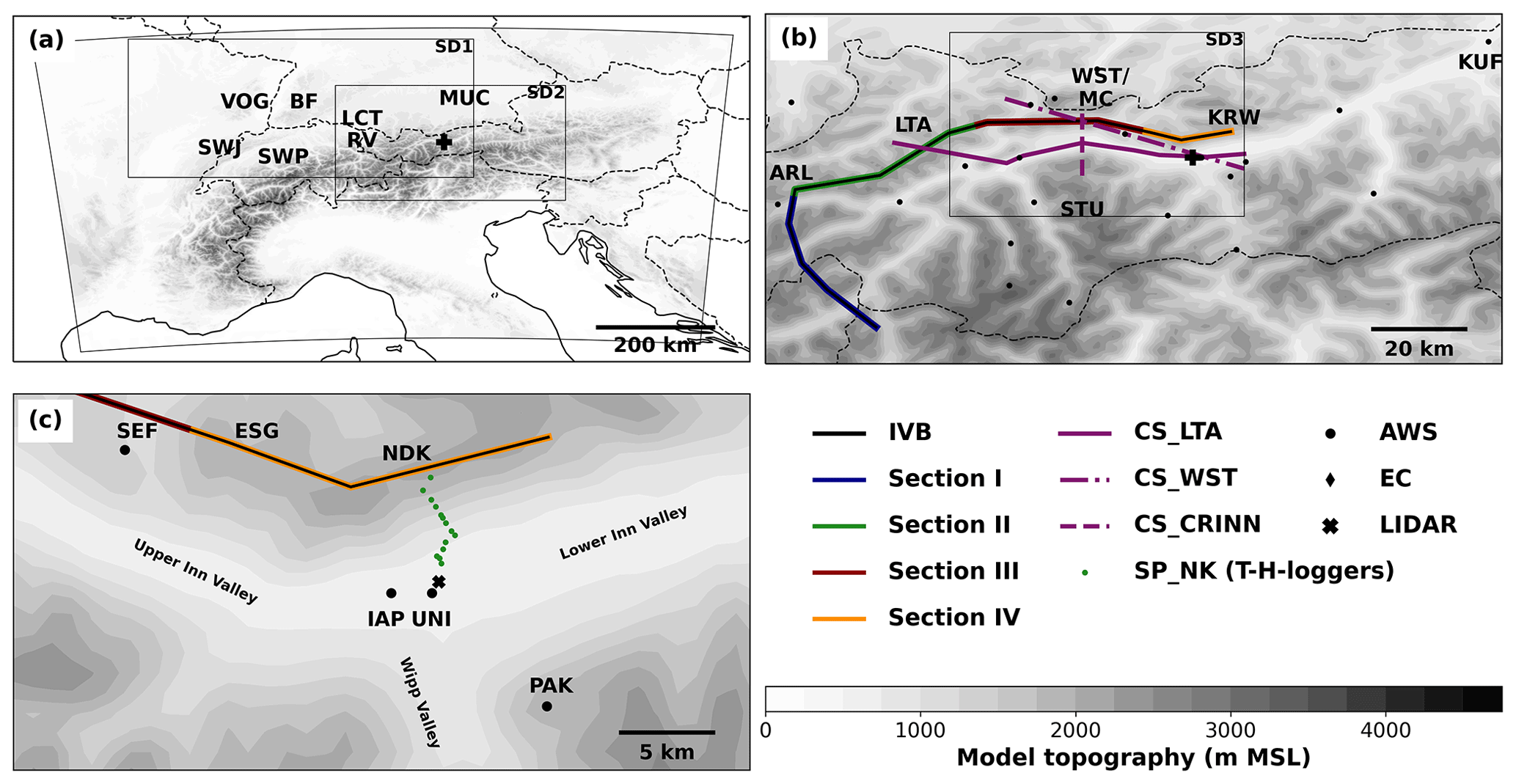
Figure 1 WRF model topography of the target area (contours, 250 m increments): (a) the full model domain, (b) the Inn Valley, and (c) the region of Innsbruck. Abbreviations describe prominent locations: Swiss Jura (SWJ), Swiss Plateau (SWP), Vosges (VOG), Black Forest (BF), Lake Constance (LCT), Rhine Valley (RV), Arlberg Pass (ARL), Lechtal Alps (LTA), Wetterstein Mountains and Mieming Chain (WST/MC), Karwendel (KRW), Stubai Alps (STU), Kufstein (KUF), Seefeld (SEF), Erlspitze Group (ESG), Nordkette (NDK), Patscherkofel (PAK), and the locations of the valley-floor surface observations at Innsbruck Airport (IAP) and the University of Innsbruck (UNI). Innsbruck is marked by a black cross in (a) and (b). The black line in (b) and (c) marks the northern boundary of the Inn Valley (IVB) represented by the crest line between ARL and KRW, as well as the western boundary of the Inn Valley south of ARL. Colored lines indicate the subsections of IVB. Three different purple lines in (b) illustrate the locations of vertical cross sections. Locations of observation sites are indicated by black symbols in (b) and (c) according to the observation type. Green dots indicate the stations of the slope profile along NDK (SP_NK). National borders are depicted as dashed black lines in (a) and (b). Subdomains SD1, SD2, and SD3 are indicated by black rectangles in (a) and (b). In the figures, MSL signifies above mean sea level.

One prominent region of foehn research has been the Inn and Wipp valleys around Innsbruck, Austria, with a research history dating back to the 19th century (Seibert, 2012). Since then almost all the research in this area has been focusing on south foehn (e.g., Zängl, 2003; Mayr et al., 2007; Umek et al., 2021), i.e., a flow originating south of the Alps, passing the main Alpine crest at the Brenner Pass and reaching Innsbruck in the west–east aligned Inn Valley via the south–north aligned Wipp Valley (Fig. 1c). Although it has been known since the early 20th century that foehn can reach Innsbruck from the north (Hann, 1891; Trabert, 1903), there has been only very little research on the topic since then. Apart from these old publications, published research comprises an observational case study by Wankmüller (1995), a climatology by Haas (2006), and one case study by Zängl (2006) based on numerical simulations. This limited amount of research is the reason that there is still a lack of understanding of the phenomenon. Especially the origin of the air mass and the penetration mechanisms of the foehn into the Inn Valley are still widely unclear (Zängl, 2006). This knowledge gap also impedes a clear-cut classification into north foehn in the case of large-scale northerly flow above crest level but westerly flow in the Inn Valley.

A peculiarity of this type of foehn in Innsbruck is that it barely ever reaches the valley bottom directly from the north via the mountain range of Nordkette (Haas, 2006; see Fig. 1c for the location). The height and steepness of this mountain range, the lack of topographic gaps, and the stable stratification of the valley atmosphere usually prevent penetration of the flow directly from the north to the valley floor. More often the flow gets channeled by the Inn Valley and appears as a strong westerly to northwesterly wind in Innsbruck (Haas, 2006). As a result of this channeling by the Inn Valley, different authors have used different expressions and different definitions for the phenomenon. Trabert (1903) and Wankmüller (1995) called the phenomenon northwest foehn and north foehn, respectively, mainly based on the measured local wind direction in Innsbruck. Investigating the same case as Wankmüller (1995), Zängl (2006) used the expression north foehn but suggested that the case should rather be referred to as northwest foehn due to the absence of a cross-Alpine gradient in pressure or temperature. Haas (2006) used a definition pointing in the same direction, making a distinction between north and west foehn based on whether or not there is a cross-Alpine flow. This was decided based on the wind direction and speed in the Wipp Valley both at the valley bottom and at crest level, as well as on the pressure difference between the northern Alpine foreland and Innsbruck. Apart from these local and large-scale approaches, the more intuitive approach based on air mass origin and prominent locations of foehn penetration has not been considered so far. For the sake of simplicity we will refer to this phenomenon as north foehn in the remainder of this section. However, we will show later whether this description is appropriate for the foehn event examined in this study.

According to Haas (2006), the relative frequency of north foehn in Innsbruck is about 1 % derived from 10 min observations recorded over a period of 5 years (1.3 % at the station Innsbruck Airport, 0.7 % at the station Innsbruck University). Therefore, north foehn occurs less frequently than south foehn, which has a relative frequency of about 5 % (Föst, 2006). North foehn in Innsbruck exhibits a pronounced annual and daily cycle with three frequency peaks in the afternoon hours of late winter, late autumn, and early summer (Haas, 2006). This frequency pattern can also be found for north foehn at stations south of the main Alpine crest (Verant, 2006; Cetti et al., 2015).

Using numerical simulations, Zängl (2006) confirmed the aforementioned channeling of the foehn flow in the Inn Valley. Based on an Eulerian model perspective, he speculated that the foehn entered the Inn Valley via the Arlberg Pass and the Silvretta Pass at the western end of the Inn Valley and possibly also in the lee of the Lechtal Alps. As already found for south foehn, vertically propagating large-amplitude gravity waves appeared to play an essential role in the penetration of the flow into the valley.

Despite the striking features in Zängl's simulations, a purely Eulerian view on the wind field does not allow for definite statements on the air mass origin. This gap can be filled, for example, by a mass flux analysis (e.g., Dautz, 2010; Arduini et al., 2020; Sabatier et al., 2020) or by a trajectory analysis. Especially trajectories have revealed complex three-dimensional flow patterns in the context of foehn winds with different flow branches upstream of the mountains (e.g., Elvidge et al., 2015; Takane et al., 2015; Würsch and Sprenger, 2015; Miltenberger et al., 2016; Jansing and Sprenger, 2020). By analyzing the heat and moisture budgets along the trajectories, the importance of various diabatic and adiabatic processes along the transport pathway can be assessed. Based on these methods, several studies have detected source regions of moisture (Langhamer et al., 2018; Schuster et al., 2021) and quantified the contribution of different processes to heat events in metropolitan areas of Japan (Ishizaki and Takayabu, 2009; Takane et al., 2013, 2015) and melt events in polar regions (Elvidge et al., 2015; Zou et al., 2019; Hermann et al., 2020; Zou et al., 2021). By separating the individual terms in the temperature tendency equation, Elvidge and Renfrew (2016) and Miltenberger et al. (2016) were able to assess the role of diabatic and adiabatic processes in foehn warming.

Apart from the uncertainties in the origin of the air mass, there is some disagreement on the role of precipitation in the development of north foehn. Haas (2006) found that in 20 % of the times north foehn in Innsbruck was associated with measurable precipitation in the Inn Valley. In 40 % of the times precipitation occurred in Kufstein (KUF; see Fig. 1b), located approximately 80 km east of Innsbruck at the northern edge of the Alps. In contrast to that, Zängl (2006) showed with simulations using full and modified model physics that orographic precipitation on the northern side of the Alps inhibited the formation of north foehn in the Inn Valley. Zängl (2006) reasoned that precipitation falling into layers of unsaturated air in the valley stabilized these layers due to evaporative cooling. This dampened the amplitude of gravity waves and thus prevented the foehn from penetrating into the valley. Similar effects were observed also in Durran and Klemp (1983) and Zängl and Hornsteiner (2007).

On a broader scale, orographic precipitation has been shown to modulate the flow patterns also on the windward side of the mountain. Latent heat release on the windward side due to orographic lifting decreases the stability of the air. This may even prevent low-level flow splitting/blocking on the windward side by prompting flow over instead of flow around the mountain (e.g., Buzzi et al., 1998; Schneidereit and Schär, 2000; Rotunno and Ferretti, 2001; Jiang, 2003). Smith et al. (2003) and Miltenberger et al. (2016) identified a phenomenon which they termed “air mass scrambling”. In such a situation air parcels that gain latent heat on the windward side while rising over the mountain are too buoyant to descend substantially on the leeward side and remain at high altitudes. In contrast, parcels starting at higher levels that experience diabatic cooling strongly descend on the leeward side and end up at low levels.

The field campaign of the research project Penetration and Interruption of Alpine Foehn (PIANO) focused on the investigation of south foehn (e.g., Haid et al., 2020; Muschinski et al., 2020; Haid et al., 2022; Umek et al., 2021). However, the first event observed on 29 October 2017 during the first intensive observation period (IOP 1) was no south foehn. Accompanied by a very strong northwesterly synoptic-scale flow, this special type of foehn established itself as strong westerly winds in the Inn Valley and prevailed in Innsbruck between 08:00 and 15:30 UTC. The rich observational data set of PIANO, in combination with mesoscale numerical simulations and trajectory analysis, provides a great opportunity to investigate this special type of foehn in detail. The main research questions are as follows:

• Where does the foehn air reaching Innsbruck come from on a regional scale before impinging on the Alps?

• Where and how does the foehn penetrate into the Inn Valley?

• What are the characteristics of the heat and moisture budgets along the pathway both on the regional and the local scale?

• Does the trajectory analysis help to classify the case as north or west foehn?

The remainder of the paper will be structured as follows. Section 2 will describe the observational data set used in this study, as well as the setup of the numerical model and the method of the trajectory analysis. After an overview of the meteorological evolution on the large and local scale in Sect. 3, the regional aspects of the air mass origin will be investigated in Sect. 4, while Sect. 5 focuses on the local aspects of the penetration mechanisms. The results will be interpreted and discussed in the context of earlier investigations in Sect. 6.

2 Data and methods

2.1 PIANO campaign

The field campaign of the PIANO project took place in autumn and early winter of 2017 in the Wipp Valley and Inn Valley. Foehn was observed during seven intensive observation periods (IOPs). The first IOP is the subject of this study. Detailed information about the field experiment and its instrumentation can be found, for example, in Muschinski et al. (2020) and Haid et al. (2020, 2022). The observations used in the closer surroundings of Innsbruck that were used in this study are depicted in Fig. 1c. Of special interest for model verification were the automatic weather stations (AWSs) at the University of Innsbruck (UNI) and at the Innsbruck Airport (IAP). One slope profile consisting of temperature and humidity loggers covering the whole Nordkette (SP_NK) was used to characterize the stratification of the valley atmosphere. The corresponding temperature measurements were in good agreement with radiosoundings taken in the middle of the valley (Haid et al., 2020). From the four Doppler wind lidars operated during the campaign, only data from one lidar (SL88, located on a rooftop in the city center) were used to derive vertical profiles of the mean horizontal wind following Haid et al. (2020). For a larger-scale picture, data from operational AWSs distributed over Tirol (Zentralanstalt für Meteorologie und Geodynamik, 2022) and the German Alpine foreland (Deutscher Wetter Dienst, 2022) as shown in Fig. 1b were analyzed.

Depending on the availability of pressure measurements at a specific site, potential temperature θ was either calculated using the standard formula or by reducing the temperature to a reference altitude similar to Muschinski et al. (2020). The second method was applied to the observations along the slope profile SP_NK. In order to ensure comparable results with both methods the reference level was not the height of the valley floor as in Muschinski et al. (2020) but 0 m a.m.s.l. When comparing model results to observations, the same method was used for both data sets.

2.2 Setup of the numerical model

The numerical simulations in this work are carried out with the advanced research version of the Weather Research and Forecasting (WRF-AWR) model, version 4.1 (Skamarock et al., 2019). The setup of the model is close to the mesoscale simulations of Umek et al. (2021). The model consists of one single domain covering the entire Alpine region with a horizontal mesh size of Δx=1 km and 1100 × 750 points. A hybrid sigma-pressure coordinate is used with 80 vertical levels. The lowest model level is at about 10 m above ground level (a.g.l.), and the model top is at 40 hPa which corresponds to a height of about 21 km. The vertical spacing increases from Δz=20 m at the surface to Δz=400 m at the model top, which results in about 33 vertical levels below crest height of the Inn Valley. The upper 8 km act as a damping layer (Klemp et al., 2008).

Model orography, soil data, and land use data are similar to Umek et al. (2021) and are based on the Shuttle Radar Topography Mission (SRTM) digital elevation model (USGS, 2000), the Harmonized World Soil Database (HWSD;  Milovac et al., 2014), and the CORINE Land Cover inventory 2012 (European Environment Agency, 2017), respectively.

Turbulence in the planetary boundary layer (PBL) is parametrized with the Mellor–Yamada–Nakanishi–Niino (MYNN) level 3 scheme (Nakanishi and Niino, 2006) with the advection of turbulence kinetic energy (TKE) being activated. While vertical mixing is performed by the PBL scheme, horizontal diffusion is calculated in physical space (diff_opt = 2) based on a first-order closure after Smagorinsky (1963). The MYNN surface-layer scheme (Nakanishi and Niino, 2006) and the unified Noah land-surface model (Ek et al., 2003) are employed. For short- and longwave radiation the RRTMG (rapid radiative transfer model for general circulation models) scheme following Iacono et al. (2008) is used, and topographic shading and slope effects on radiation are activated. Cloud microphysics are parametrized with the Thompson scheme (Thompson et al., 2008). Convection is assumed to be fully resolved in the model and thus is not parametrized.

The operational 6-hourly high-resolution analysis of the Integrated Forecasting System (IFS) of the European Centre for Medium Range Weather Forecasts (ECWMF) is used as initial and boundary conditions. In order to correct the erroneous snow cover distribution in the ECMWF analysis, all snow below 1800 m a.m.s.l. was removed. This height of the snow line was determined from webcam images of the region west of Innsbruck. Extrapolation of the temperature field of the ECMWF analysis to WRF model levels located below the IFS topography is done with a moist adiabatic lapse rate of Γ=6.5 K km⁻¹. In contrast to Umek et al. (2021) no observation nudging was employed.

The simulation starts at 12:00 UTC on 28 October 2017 and ends at 00:00 UTC on 30 October 2017 covering the whole time span of the foehn event with a spin-up time of several hours before the main foehn period starts. In addition to the standard model output interval of 1 h, a finer output interval of 5 min is used for the main foehn phase between 00:00 and 15:00 UTC on 29 October 2017. These fields serve mainly as input for the trajectory calculations and include the three-dimensional fields of all three wind components, temperature, pressure, geopotential height, mixing ratios of water vapor and all hydrometeor classes, and subgrid-scale turbulence kinetic energy (SGS-TKE), as well as accumulated precipitation at the surface.

2.3 Trajectory analysis

2.3.1 LAGRANTO settings

The trajectory analyses are carried out with the Lagrangian analysis tool LAGRANTO version 2.0 (Sprenger and Wernli, 2015). Parcels for backward trajectories are released every hour between 06:00 and 15:00 UTC on 29 October 2017 in a volume with a square base of 3 × 3 km centered over Innsbruck and a height of 1800 m covering the altitudes between 700 and 2500 m a.m.s.l. Starting points are equally distributed in this volume with a horizontal distance of 200 m and a vertical distance of 25 m, which results in a total of 18 688 trajectories per starting time. Trajectories are calculated backward in time for 6 h. During these 6 h the parcels have traveled far enough to determine the source regions upstream of the Alps but not too far to have left the model domain. The trajectory calculation is based on the WRF wind fields available every 5 min. The integration time step is 15 s, and the output interval is 1 min. The 15 s as integration time step is chosen to ensure that no grid cell is skipped between each integration time step for all expected wind speeds, and thus all features resolved by the input wind data are represented in the trajectory (Stohl, 1998). The jump option for trajectories intersecting with the model topography is active so that these trajectories are artificially lifted above the model topography and are allowed to continue. Without this option being active, about half of the trajectories would be lost.

The 5 min input interval lies at the upper end of the range suggested, for example, by Bowman et al. (2013) and Schär et al. (2020) for kilometer-scale simulations. Experiments with different input intervals and integration time steps showed the expected error growth with decreasing temporal resolution but did not reveal a significant impact of the LAGRANTO settings on the general conclusions of this study (Saigger, 2021).

In contrast to other trajectory analysis tools like FLEXPART (Brioude et al., 2013) or HYSPLIT (Stein et al., 2015), LAGRANTO does not account for the impact of subgrid-scale turbulence on the trajectories. The calculation is solely based on the resolved wind field. Hence, the trajectories in the channeled flow in the Inn Valley below crest height are most likely less dispersive than in reality. Sensitivity experiments showed that a large number of trajectories with starting positions distributed over a whole volume is necessary for a reasonable trajectory dispersion (Saigger, 2021). Hence, the big ensemble of trajectories ensures that at least the resolved flow variability in the model is fully captured by the trajectories. Along the trajectories temperature, pressure, wind components, water vapor mixing ratio, hydrometeor mixing ratios, and SGS-TKE are traced. Additionally also the precipitation intensity at the ground below the trajectory and the terrain height are saved.

2.3.2 Additional calculations

In addition to the variables directly traced along the trajectories several other variables are diagnosed from the primary ones. The difference between the fields of accumulated precipitation of two following time steps is calculated to obtain the 5 min precipitation intensity which is then multiplied by a factor of 12 to get an hourly precipitation intensity for easier interpretation. A total water mixing ratio q_t is derived by adding up the mixing ratios of water vapor and all five hydrometeor classes of the Thompson scheme. Ice–liquid potential temperature is calculated with the approximate form following Curry (2015):

$$\begin{array}{}\text{(1)}& {\mathit{\theta }}_{\mathrm{il}}=\mathit{\theta }\exp \left(-{\displaystyle \frac{L_{\mathrm{v}}{q}_{\mathrm{l}}}{c_{p}T}}-{\displaystyle \frac{L_{\mathrm{s}}{q}_{\mathrm{s}}}{c_{p}T}}\right).\end{array}$$

Here L_v and L_s are the latent heat of evaporation and sublimation, and q_l and q_s are the mixing ratios of liquid and solid water, respectively. The ice–liquid potential temperature is defined as the potential temperature that an air parcel would have if all liquid water was evaporated and all ice particles were sublimated. For moist reversible processes, for example, cloud formation and cloud dissipation without precipitation, θ_il stays constant. Hence, a decrease in total water content increases θ_il and vice versa. For our purposes the approximate form of θ_il given by Eq. (1) is sufficient, and more accurate forms like in Bryan and Fritsch (2004) are not necessary.

Analog to Hermann et al. (2020) the adiabatic and diabatic effects on temperature along the trajectory are calculated. In the equation for the Lagrangian temperature tendency,

$$\begin{array}{}\text{(2)}& {\displaystyle \frac{DT}{Dt}}={\displaystyle \frac{\mathit{\kappa }T\mathit{\omega }}{p}}+H{\left({\displaystyle \frac{p_{\mathrm{0}}}{p}}\right)}^{-\mathit{\kappa }},\end{array}$$

the first term of the right-hand side describes the adiabatic heating or cooling along the trajectory with the Lagrangian pressure tendency $\mathit{\omega }=\frac{Dp}{Dt}$ and $\mathit{\kappa }=R/c_p=\mathrm{0.286}$. The second term represents the diabatic heating or cooling with $H=\frac{D\mathit{\theta }}{Dt}$. Following Hermann et al. (2020) Eq. (2) can be discretized as

$$\begin{array}{}\text{(3)}& \begin{array}{rl}{\left.{\displaystyle \frac{DT}{Dt}}\right|}_{t=t_i}& \approx {\displaystyle \frac{T_i-T_{i-\mathrm{1}}}{\mathrm{\Delta }t}}\approx \mathit{\kappa }\left({\displaystyle \frac{T_i+T_{i-\mathrm{1}}}{p_i+p_{i-\mathrm{1}}}}\right)\left({\displaystyle \frac{p_i-p_{i-\mathrm{1}}}{\mathrm{\Delta }t}}\right)\\ & +{\displaystyle \frac{{\mathit{\theta }}_i-{\mathit{\theta }}_{i-\mathrm{1}}}{\mathrm{\Delta }t}}{\left({\displaystyle \frac{\mathrm{2}{p}_{\mathrm{0}}}{p_i+p_{i-\mathrm{1}}}}\right)}^{-\mathit{\kappa }},\end{array}\end{array}$$

where variables with subscript i refer to time t=t_i and subscript i−1 to time $t=t_i-\mathrm{\Delta }t$. Δt denotes the time interval between the individual trajectory points: in our case Δt=1 min which represents the output interval (see Sect. 2.3.1). In contrast to Hermann et al. (2020) the adiabatic term (first term on right-hand side of Eq. 3) is calculated explicitly and not as a residual term.

The spatial distribution of trajectory properties is determined by interpolating these properties from the trajectory position to a Cartesian grid with a horizontal mesh size of 3 km. This mesh size is larger than the grid point distance of the WRF domain in order to ensure that trajectories do not “skip” grid boxes between two time steps at which the trajectory positions are known (1 min interval). For the calculation of the trajectory density the proportion of trajectories with at least one point within the grid box is determined. If a certain trajectory has more than one point within the same grid box, it is only counted once. Similarly median trajectory properties are calculated on the same grid by taking the median of various parameters (e.g., trajectory height) over all trajectories within one grid box. To ensure that all trajectories are weighted equally, independent on the number of points within the grid box, first the median for all points of one trajectory in this grid box is calculated. Subsequently, these median properties are averaged over all individual trajectories within the grid box. For temperature and moisture variables not only the local value but also the difference to the value at the arrival in Innsbruck is calculated and gridded in order to quantify heat and moisture gain or loss along the trajectories.

An appropriate valley boundary has to be defined in order to determine the point where the trajectories penetrate into the Inn Valley (see line IVB representing the Inn Valley boundary in Fig. 1b, c). In the north of the Inn Valley this boundary essentially follows the crest line. South of the Arlberg Pass the line IVB is defined by the western end of the Inn Valley and its tributaries. For each trajectory the point where the valley boundary is first crossed is determined with a resolution of 1 km along the valley boundary. For later investigations the valley boundary is divided into four sections with distinct topographic features (see Fig. 1b, c). Section I covers the western end of the Upper Inn Valley, the Paznaun Valley with the Silvretta Pass, and the Arlberg Pass. Section II contains the ridge line of the Lechtal Alps until the region of Fern Pass. Section III covers the two mountain saddles of Fern Pass and Seefeld with the Wetterstein Mountains and Mieming Chain in between, while Section IV stretches out over the Karwendel and includes its most western part of the Erlspitze Group (ESG) next to Seefeld, as well as the Nordkette directly north of Innsbruck (NDK; see Fig. 1c).

3 Meteorological overview

3.1 Synoptic and mesoscale analysis

On 29 October 2017 a pronounced low-pressure system was located over northeastern Europe (Fig. 2a). The associated jet stream led to strong northwesterly flow towards the Alps. The lower troposphere north of the Alps was characterized by a pronounced elevated temperature inversion at around 1500 m a.m.s.l. as depicted by the radiosonde profile of Munich at 00:00 UTC (not shown). Below this inversion the flow was deflected eastward by the Alps, while above crest level the flow crossed the Alps (Fig. 2c). The deflected flow is depicted in Fig. 2c by the observations at Munich and Kempten, as well as at the station of Hohenpeissenberg, a 977 m a.m.s.l. high mountain in the Alpine foreland. The mountain top stations of Zugspitze, Patscherkofel, and Rudolfshütte illustrate strong cross-Alpine flow with strong north to northwesterly winds, while for stations like Valluga and Brunnenkogel local flow deflection may explain the stronger westerly wind component. With the pressure low moving south and an embedded short-wave trough approaching the Alps, crest-level winds further intensified during the morning of 29 October 2017 with mean wind speeds of about 20 m s⁻¹ at Zugspitze and around 15 m s⁻¹ at Patscherkofel. Orographic precipitation on the northern side of the Alps already occurred in the night and the morning before the cold front arrived in the afternoon (Fig. 2d). The high precipitation intensities were restricted to the stations at the very northern edge of the Alps with locally more than 10 mm of precipitation between 00:00 and 12:00 UTC on 29 October 2017. A clear precipitation shadow can be detected in the Inn Valley with observed precipitation not exceeding 5 mm during the same period.

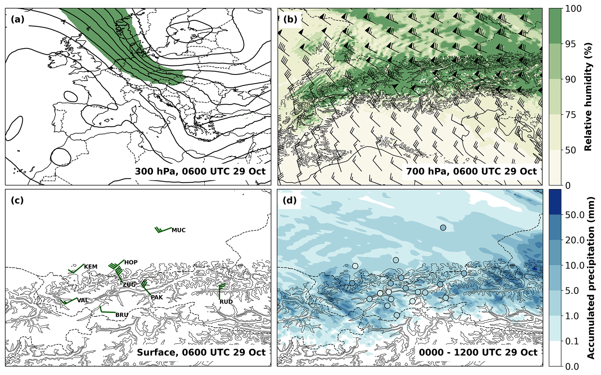
Figure 2 Synoptic situation on 29 October 2017. (a) ECMWF analysis of geopotential (black contour lines, spacing 1000 m² s⁻²) and wind speed (shading, wind speed greater than 50 m s⁻¹ is shaded in green) at 300 hPa at 06:00 UTC. (b) WRF simulated fields of wind (barbs) and relative humidity (color contours) at 700 hPa at 06:00 UTC. (c) Observed winds (barbs) at 06:00 UTC. Abbreviations indicate station names: Munich (MUC), Kempten (KEM), Hohenpeissenberg (HOP), Zugspitze (ZUG), Valluga (VAL), Brunnenkogel (BRU), Patscherkofel (PAK), and Rudolfshütte (RUD). (d) Precipitation accumulated between 00:00 and 12:00 UTC in subdomain SD2 simulated by WRF (color contours) and observed (filled circles with the same color scale). National borders are as in Fig. 1, and model topography in (b)–(d) is indicated by black contour lines for the elevations of 1000 and 1500 m a.m.s.l. Wind barbs in (b) and (c) indicate the wind speed (in kn): half barb, full barb, and triangle denote 2.5, 5, and 25 m s⁻¹.

The WRF simulation reproduces the deflected flow at lower levels (not shown) and the near-crest-level flow crossing the Alps reasonably well (Fig. 2b). As in the observations, the strongest precipitation is simulated at the northern edge of the Alps, as well as over the higher inner-Alpine mountain ranges (Fig. 2d). The simulated amounts are in the same range as the maximum observed values. The simulation also captures the rain shadow in the valleys.

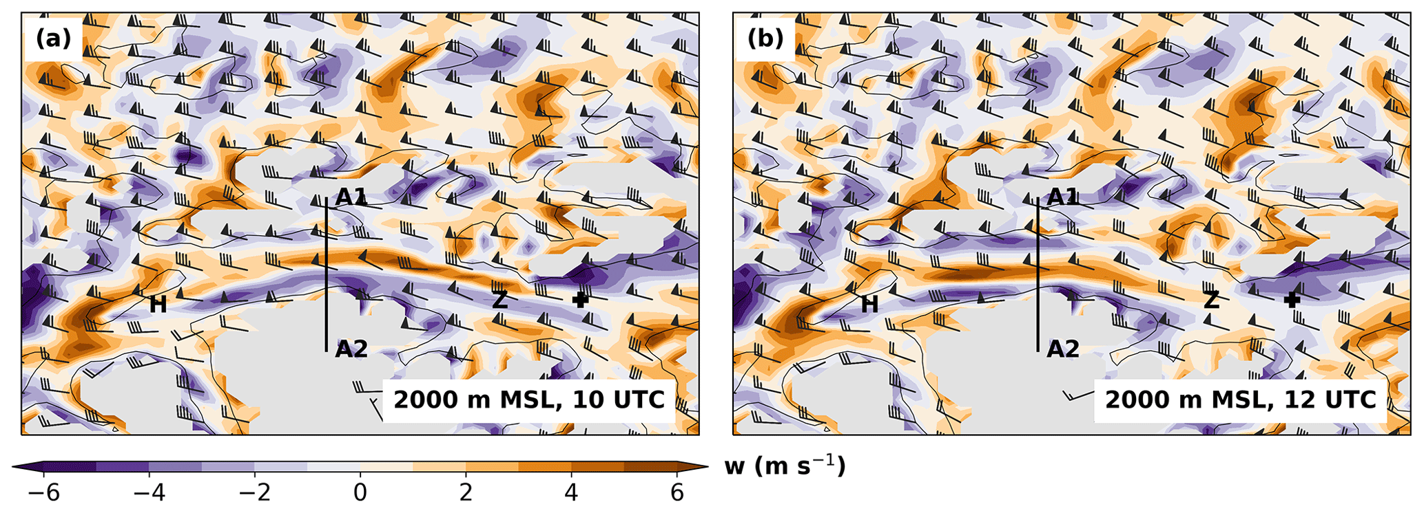
Figure 3 Simulated horizontal wind and vertical velocity at 2000 m a.m.s.l. at (a) 10:00 UTC and (b) 12:00 UTC on 29 October 2017 in subdomain SD3. Horizontal wind is depicted by wind barbs as in Fig. 2b, vertical velocities are illustrated by color contours. Model topography is indicated by black contour lines for the elevation of 1500 m a.m.s.l., and areas with model topography higher than 2000 m a.m.s.l. are shaded in grey. Locations of Haiming (H) and Zirl (Z) are indicated by letters, the location of Innsbruck is indicated by a black cross. The orientation of the vertical cross section CS_CRINN is depicted by a thick black line with A1 and A2 being the start and end points of the cross section as in Fig. 4.

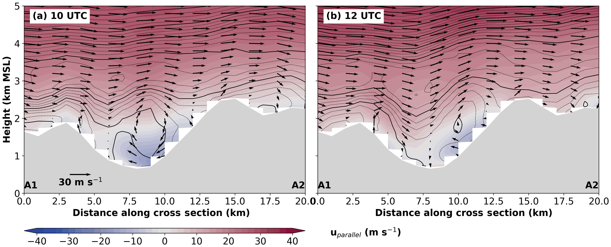
Figure 4 Vertical transect of simulated equivalent potential temperature (black contour lines: spacing 2 K for thick solid lines and spacing 0.5 K for thin dashed lines) and wind field (color contours and arrows) along cross section CS_CRINN at (a) 10:00 UTC and (b) 12:00 UTC on 29 October 2017. Color contours represent the horizontal wind component parallel to the plane (positive towards right), arrows illustrate the two-dimensional wind field on the vertical plane. Model topography is shaded in grey. A1 and A2 in (a) and (b) mark the start and end point of the transect as depicted in Fig. 3.

The cross-Alpine flow formed a complex pattern of gravity waves. While during the first half of the night trapped lee waves with rather short wavelengths dominated in the Inn Valley region (not shown), horizontal wavelength increased in the second half of the night. In the morning the crest-level flow field east of Innsbruck was dominated by a single gravity wave over the Inn Valley with subsiding motion on the northern slopes and rising motion on the southern slopes (Fig. 3a). In contrast, the flow field west of Innsbruck was dominated by an atmospheric rotor that was situated underneath a gravity wave and covered the whole valley cross section (Fig. 4a). This rotor led to subsiding motion on the southern side of the valley and rising motion on the northern side and stretched out in a roughly 30 km long section along the Inn Valley between Haiming and Zirl (see dipole structure between H and Z in Fig. 3a). The rotor was dominant in this region between 06:00 and 11:00 UTC. Later, crest-level winds shifted to a slightly stronger northerly component (Fig. 3b), and the horizontal wave length and the amplitude of the lee wave increased. This led to a weakening and shift in the position of the rotor and to stronger subsidence on the northern slopes of the Inn Valley (Figs. 3b, 4b).

3.2 Local analysis

The observations show that the ambient northwesterly flow was channeled into a westerly flow inside the valley (Fig. 5a). During the night the lower valley atmosphere was still decoupled from the flow aloft with low wind speeds and a stable stratification up to about 1500 m a.m.s.l. Light precipitation was measured at the surface (not shown). During the morning hours the foehn gradually descended down and broke through in Innsbruck at the valley floor at about 08:00 UTC (Fig. 5a). The valley atmosphere was still slightly stably stratified based on dry potential temperature. After around 10:00 UTC the whole valley atmosphere was well mixed (Fig. 5a). The vertical profile of the horizontal wind above Innsbruck exhibited a low-level jet structure with a maximum at around 800 m a.m.s.l. and a local minimum at about 1200 m a.m.s.l. (Fig. 5a). After around 11:00 UTC winds above crest height weakened slightly, and, with the advection of potentially colder air, also the westerlies inside the valley lost strength. At the surface this cooling manifested itself with two distinct drops in temperature at about 11:30 and 13:30 UTC before the arrival of the cold front at 15:30 UTC (Fig. 6a). The cold front arrived in Innsbruck from the lower Inn Valley, filling the valley with potentially colder air and forcing the westerlies to lift off the surface (Fig. 5a). In the later phase also flow directly from the north could be observed in the middle of the valley atmosphere (Fig. 5a).

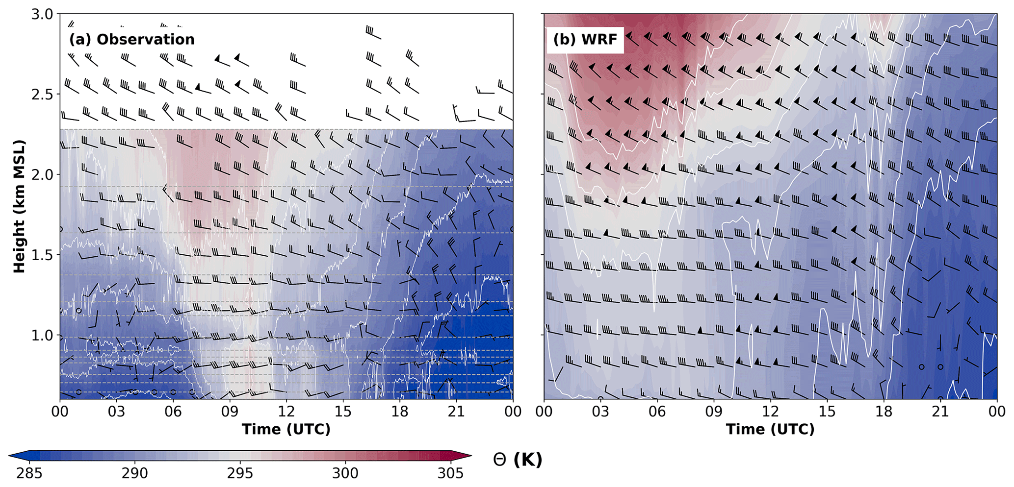
Figure 5 Time–height diagram of (a) observed and (b) simulated potential temperature and mean horizontal wind in Innsbruck on 29 October 2017. Potential temperature is shown by color contours and white contour lines with a spacing of 2 K, wind barbs indicate wind speed and direction as in Fig. 2. Temperature measurements were conduced along the slope profile SP_NK, and gray horizontal lines indicate the measurement heights. Wind barbs are shown at an hourly interval and represent 10 min averages of the horizontal wind measured with the Doppler wind lidar SL88. Potential temperature and wind in (b) are 10 min averages of the time series of every integration time step at the WRF grid point closest to UNI.

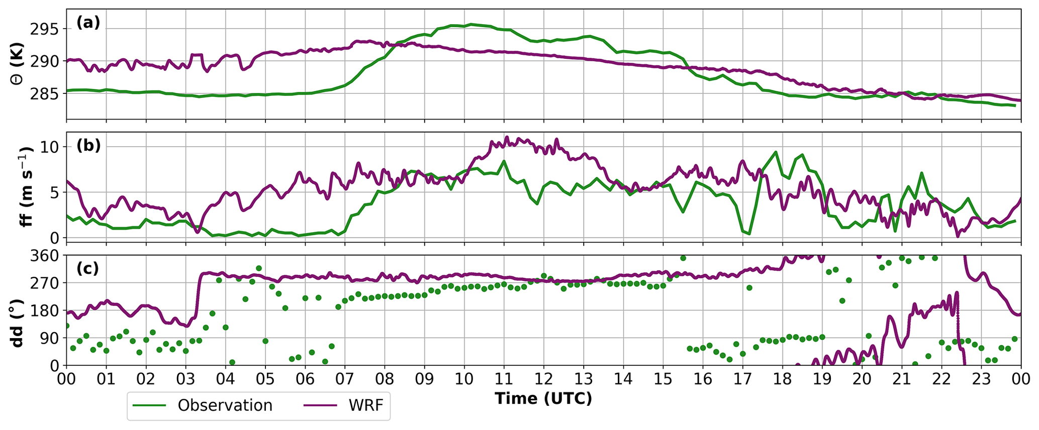
Figure 6 Temporal evolution of (a) potential temperature, (b) wind speed, and (c) wind direction at the University of Innsbruck (UNI) on 29 October 2017. Observations are depicted in green and represent 10 min measurements. Model results are depicted in purple as a time series at every integration time step at the WRF grid point closest to UNI.

Figure 5 illustrates that the WRF simulation captures the overall flow pattern of the fully developed foehn in the valley reasonably well with the northwesterly flow being channeled to a westerly wind below crest height. However, during the night the simulated pre-foehn cold-air pool (CAP) is too shallow and not strong enough to decouple from the flow aloft (Fig. 5b). This leads to strong westerlies inside the valley throughout the whole night (Fig. 5b) with a warm bias at the surface of about 5 K (Fig. 6a). The weak CAP stratification in the model causes a breakthrough of the foehn that is too early in Innsbruck. Here, the foehn reaches the valley bottom almost 4 h earlier in the model than in reality which can be seen by the shift to westerlies and the increase in wind speed (Fig. 6c). Once the foehn is fully established in both the model and in reality the model exhibits a cold bias of about 4 K over the whole neutral layer covering the lowest 1000 m of the valley. Wind speeds in the model are generally higher both above crest height and within the valley (Fig. 5). In agreement with the observations, the model depicts a local wind maximum at about 500 m above the valley surface (Fig. 5b) which is even more pronounced at locations further upstream in the Inn Valley (not shown). The simulated foehn is strongest between about 11:00 and 13:00 UTC both at the surface (Fig. 6b) and throughout the whole valley atmosphere (Fig. 5b). The cooling of the foehn flow in the early afternoon is captured by the WRF simulation, as well as the strong cold air advection by the cold front.

In summary, the WRF simulation captures large parts of the mesoscale evolution reasonably well. The regional flow patterns and the precipitation pattern over the Alps are in good agreement with the observations with the exception of wind speeds that are generally too high. During nighttime, the model does not correctly reproduce the CAP in the Inn Valley and the associated decoupling of the upper-level flow. However, once the foehn is fully established inside the valley, the simulated flow patterns are in better agreement to the observations, with the exception of a cold bias of about 4 K in the model. These two problems have been observed frequently for mesoscale simulations of foehn flows (e.g., Gohm et al., 2004; Zängl et al., 2004; Zängl, 2006; Wilhelm, 2012; Sandner, 2020; Umek et al., 2021). A common explanation for this is a possible misrepresentation of turbulent mixing in those models. The simulation is sufficiently good to be used for the subsequent trajectory analysis especially since the main focus is on the fully developed foehn phase during which the model discrepancies are minor.

4 Air mass origin and history

4.1 Air mass origin

Based on the findings in Sect. 3 the following trajectory analysis concentrates on distinct phases of the foehn event. Special emphasis is placed on the phase around 10:00 UTC on 29 October 2017, when foehn is fully established both in the model and in reality and when model and observations are (with the aforementioned exceptions like the cold bias) in reasonable agreement. A second focus is put on the phase around 12:00 UTC, when the strongest winds are simulated and when there is a change in the gravity wave pattern over the Inn Valley. To get a more complete picture, a short analysis is done for the whole foehn period between 06:00 and 15:00 UTC. In general, all analyses are restricted to trajectories reaching the valley atmosphere above Innsbruck between 700 and 1700 m a.m.s.l. This is the well-mixed layer characterized by a nearly dry adiabatic lapse rate (Fig. 5b). Therefore all trajectories that arrive in this layer can, in principle, reach the valley floor by vertical turbulent mixing, an effect that is not explicitly taken into account in the trajectory model LAGRANTO.

Figure 7 Gridded field in subdomain SD1 of trajectory density for trajectories arriving in Innsbruck at 10:00 UTC on 29 October 2017 between 700 and 1700 m a.m.s.l. Trajectories are calculated 6 h backward in time. Trajectory density as explained in Sect. 2.3.2 is indicated by color contours. Model topography is depicted outside the trajectory plume by gray shading as in Fig. 1 and inside by black contour lines of the elevations of 1000 and 1500 m a.m.s.l. National borders are shown as in Fig. 1. The latitude of 47.2^∘ N separating the two main trajectory branches is marked by a dashed black line. The northern (southern) branch represents 75 % (25 %) of all trajectories.

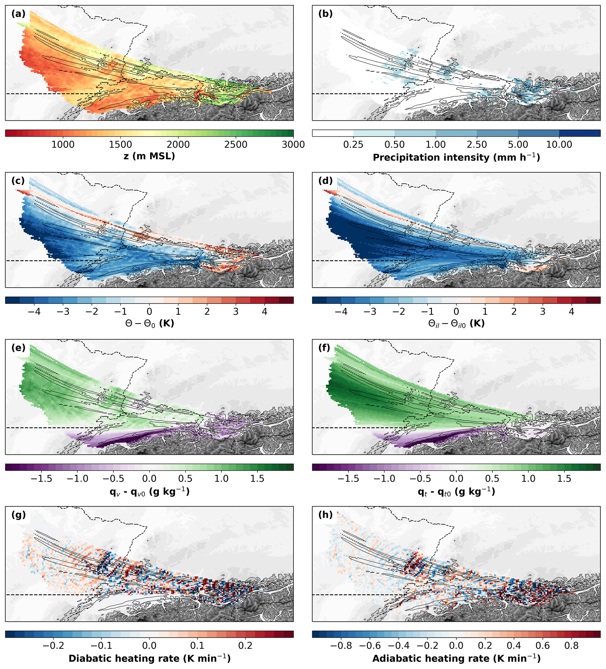
Figure 8 Gridded fields in subdomain SD1 of various trajectory properties for trajectories as shown in Fig. 7. Depicted are the median of (a) trajectory height, (b) precipitation intensity at the surface, (c) potential temperature deviation, (d) ice–liquid potential temperature deviation, (e) water vapor mixing ratio deviation, (f) total water content deviation, (g) diabatic heating rate, and (h) adiabatic heating rate. All deviations refer to the corresponding reference value at the trajectory arrival point Innsbruck. Trajectory properties are indicated by color contours, model topography and national borders are as in Fig 7, and main flow branches are indicated by the contour line of a trajectory density of 0.03 (thin black line). The latitude of 47.2^∘ N separating the two main trajectory branches is marked by a dashed black line.

Figure 7 shows that the foehn air reaching Innsbruck at 10:00 UTC on 29 October 2017 has its main origin 6 h earlier distributed over a wide region in the northwestern part of the model domain in eastern France (about 75 % of all trajectories). A second major branch representing about 25 % of the trajectories (Fig. 7) originates in the northern part of Switzerland south of the mountains of the Swiss Jura. Both major flow branches funnel towards the Alps and impinge on the mountains in the area around Lake Constance and the Rhine Valley. As will be seen later in Sect. 4.2 the trajectories of the northern branch and the ones of the southern branch experience very different diabatic processes; therefore they are analyzed separately in the following. The separation into a northern and a southern branch is based on the trajectory of the starting latitude 6 h before the arrival which is either north or south of 47.2^∘ N. This reference latitude has been chosen manually based on the density distribution shown in Fig. 7 and the moisture fields in Fig. 8e and f.

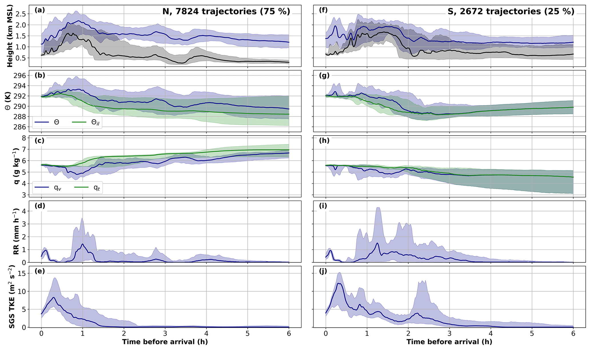
Figure 9 Temporal evolution of trajectory properties for trajectories as shown in Fig. 7 starting north (left column) and south of 47.2^∘ N (right column). Thick lines indicate the median and shadings the 10th and 90th percentile. (a, f) Trajectory height (blue) and terrain height (black) (in km a.m.s.l.); (b, g) θ (blue) and θ_il (green) (in K); (c, h) q_v (blue) and q_t (green) (in g kg⁻¹); (d, i) precipitation intensity at the surface (in mm h⁻¹); and (e, j) subgrid-scale (SGS) TKE (in m² s⁻²).

The trajectories starting in France are mainly concentrated into one air stream that crosses the mountain ranges of the Vosges and the Black Forest about 4 and 3 h, respectively, before the arrival in Innsbruck. Finally, the air stream reaches the Alps near Lake Constance about 1.5 h before the arrival in Innsbruck (Fig. 7 and Fig. 9a). The major part of these trajectories, more than 80 % (see Fig. 9a), start concentrated within a narrow layer between 1000 and 1500 m a.m.s.l. However, secondary air streams originating from higher levels also play a role (Fig. 8a). The trajectories pass the Vosges and the Black Forest mountains on a nearly terrain-following path with an average height of about 1000 m above the local topography (Fig. 9a). Thus, the trajectories get lifted by about 200 m at the Vosges and by about 500 m at the Black Forest. In the lee of the Vosges the trajectories experience a strong wave signal with two wave troughs parallel to the mountain crest (Fig. 8a). A minor part of the trajectories originating from France starts further south at a slightly lower altitude of about 1000 m a.m.s.l. (Fig. 8a). Part of these trajectories do not cross the Vosges and the Black Forest but pass them laterally in the south and funnel into the main air stream before reaching the Alps.

About 25 % of the trajectories reaching Innsbruck at 10:00 UTC on 29 October in the lower valley atmosphere can be assigned to the southern branch from Switzerland (see Fig. 9). Starting over the Swiss Plateau at about 1200 m a.m.s.l. the air stream is first parallel to the northern Alpine rim and ultimately impinges on the Alps near the Rhine Valley at a median altitude of about 1300 m a.m.s.l. about 2 h before the arrival in Innsbruck (Fig. 9f). When crossing the Alps, trajectories of both flow branches are lifted to heights between 2000 and 2500 m a.m.s.l.

4.2 Diabatic processes

4.2.1 Origin north of 47.2^∘ N

The air along the trajectories starting north of 47.2^∘ N experiences a mean diabatic heating of about 2.5 K in terms of potential temperature and loses on average about 1 g kg⁻¹ of water vapor and about 1.3 g kg⁻¹ of total water content by the arrival in Innsbruck (Fig. 9b, c). This is especially true for the trajectories within the main air stream. Those starting at lower levels further south in France experience a much stronger warming of 5 K and a moisture loss of up to 2 g kg⁻¹. The ones originating from higher levels start potentially warmer and thus are diabatically cooled by about 3 to 5 K during their journey to Innsbruck but only lose about 0.5 g kg⁻¹ of total water content (Fig. 8c, e, f). For the main air stream the strongest adiabatic and diabatic temperature changes occur while crossing the mountain ranges of the Vosges, the Black Forest, and the Alps. The diabatic and adiabatic heating rates are strongly anticorrelated. Adiabatic cooling is taking place when the air parcels are being lifted on the windward side of the mountain ranges due to expansion, while at the same time diabatic warming is taking place. The opposite can be observed during subsidence on the leeward side (Figs. 8a, c, g, h and 9a, b). These diabatic temperature changes are associated with moisture changes. On the windward side of the mountain ranges a decreasing water vapor mixing ratio points towards the formation of hydrometeors and thus diabatic heating due to latent heat release. The opposite is happening on the leeward side with increasing water vapor mixing ratios due to evaporation of the hydrometeors and consequently evaporative cooling (Figs. 8c, e and 9b, c). It is noteworthy that adiabatic and diabatic temperature changes occur not only in the immediate vicinity of the major mountain ranges but also further downstream as a result of the vertical motions of trapped lee waves (Fig. 8g, h).

With the passing of all three mountain ranges a net warming in terms of potential temperature and a decrease in total water content can be observed (Figs. 8c, f and 9b, c). Between the start of the trajectories and their arrival at the Alps a net diabatic heating of about 1.5 K has taken place with about 0.5 K of net warming at the Vosges and 1 K at the Black Forest (Fig. 9b). After the flow has reached the Alps a further net increase in potential temperature of about 1 K can be observed (Fig. 9b). All three net increases in θ are accompanied by an increase in θ_il (Figs. 8d and 9b), which illustrates that the heating is due to irreversible moisture loss associated with orographic precipitation (Figs. 8b, f and 9c, d). While the net warming is approximately the same when crossing the Black Forest and the Alps, the changes in θ_il and q_t, as well as the precipitation intensity at the surface, are much stronger in the case of the Alps. At the same time, SGS-TKE along the trajectories is nearly zero over the pre-Alpine terrain but strongly increases over the Alps up to mean values of about 8 m² s⁻² (Fig. 9e). These high TKE values suggest that turbulent mixing is a non-negligible heating/cooling source over the Alps. However, this effect can not be quantified in this study.

4.2.2 Origin south of 47.2^∘ N

Compared to the northern trajectory branch, the air along the southern branch experiences a similar net diabatic heating of about 2 K (Figs. 8c and 9g). However, the ways in which this heating is achieved are quite different. The air along the northern branch loses moisture along the way, and large parts of the diabatic heating can be explained by latent heat release during the formation of orographic precipitation. In contrast, the air of the southern branch gains moisture of about 1 g kg⁻¹ on average (Figs. 8f and 9h).

This moisture gain and the diabatic temperature changes occur at several different spots during the journey of the air masses. During the first hours over the Swiss Plateau diabatic heating rates are almost zero (Fig. 8g). However, the comparatively dry air parcels directly north of the Alpine rim (Fig. 8e, f) already gain about 1 g kg⁻¹ of moisture in the first 3 h of their journey (see 10th percentile in Fig. 9h). West of the Rhine Valley all trajectories experience a moistening presumably due to precipitation formed at higher levels that partly evaporates at lower levels where the trajectories are located (Figs. 8b and 9h, i). At the beginning, this is consistent with a decrease in θ_il. From 2.5 h before the arrival, however, the increasing θ_il in combination with the increasing moisture suggests the occurrence of compensating diabatic processes (Fig. 9g). With the lifting at the Alps the presumably local formation of hydrometeors leads to diabatic heating in terms of potential temperature (Fig. 9f–h). During the flow over the Alps an increase in θ_il shows irreversible diabatic heating (Fig. 9g). However, the near-constant total water content, together with the non-zero precipitation and SGS-TKE (Fig. 9h–j), points towards a complex interplay of processes like turbulence and three-dimensional moisture exchange that can not be fully disentangled in this study.

In summary, the foehn air reaching Innsbruck at 10:00 UTC on 29 October 2017 experiences strong diabatic processes along the way. Depending on the origin of the air parcels, a very different history in terms of diabatic processes can be observed. Large parts of the diabatic temperature changes and moisture changes can be explained by the formation of orographic precipitation. However, with the flow impinging on the Alps, the flow pattern gets more complex, and turbulent processes, as well as three-dimensional moisture exchanges, appear to play an important role. However, these processes can not be disentangled and quantified with our methods. Therefore, a complete assessment of all processes is not possible within this study.

4.3 Temporal evolution

In the previous sections the analysis concentrated on trajectories arriving in Innsbruck at 10:00 UTC on 29 October. This section will analyze the evolution over the whole foehn period between 06:00 and 15:00 UTC.

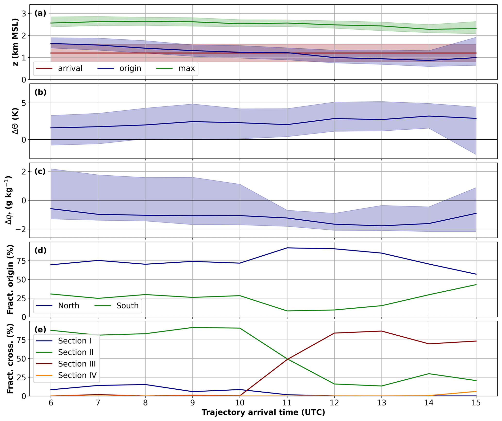
Figure 10 Temporal evolution of trajectory properties for trajectories arriving in Innsbruck from 06:00 to 15:00 UTC on 29 October 2017 between 700 and 1700 m a.m.s.l. Upstream conditions are averages between 5 and 6 h before the arrival in Innsbruck. (a) Upstream trajectory height (blue), maximum trajectory height (green), and trajectory arrival height in Innsbruck. The distribution of the arrival height in Innsbruck is indicated in red. Difference in (b) potential temperature and (c) total water content between the upstream condition and at the arrival in Innsbruck. The median in (a)–(c) is indicated by a thick line and the range between the 10th and 90th percentile as color shading. (d) Fraction of trajectories starting either north (blue) or south (green) of 47.2^∘ N. (e) Fraction of trajectories crossing the Inn Valley boundary at four different sections as defined in Sect. 2.3.2.

Based on Fig. 10 three phases can be identified. The first phase spans from 06:00 to 10:00 UTC with a relatively constant trajectory fraction of about 75 % (25 %) originating north (south) of 47.2^∘ N (Fig. 10d). This phase is further characterized by a mean diabatic heating of about 2 K in terms of potential temperature and a total moisture loss of about 1 g kg⁻¹ (Fig. 10b, c). While on average the air loses moisture, part of the air actually gains moisture (see positive values of the 90th percentile in Fig. 10c). Throughout this phase the height of the air mass origin upstream of the Alps constantly decreases from about 1700 to 1200 m a.m.s.l., while the maximum trajectory height over the Alps stays approximately constant. It is noteworthy that at the end of the first phase the median trajectory height upstream and at the arrival in Innsbruck are about the same.

The second phase between 11:00 and 13:00 UTC is characterized by an even higher contribution of the northern trajectory branch of up to 90 % (Fig. 10d). At the same time, the average diabatic heating and the total moisture loss sightly increase compared to the previous phase (Fig. 10b, c). After 11:00 UTC nearly all trajectories experience a moisture loss as indicated by the negative 90th percentile in Fig. 10c. This is consistent with the decreasing contribution of the southern trajectory branch (Fig. 10d). However, while this trajectory branch was earlier characterized by a net uptake of moisture, now the net change in moisture is about zero due to increased moisture loss at the Alps (not shown). The maximum trajectory height slightly decreases to about 2400 m a.m.s.l. at 13:00 UTC. At the same time, the decrease in the height of the air mass origin continues also in this second phase of the event. On average, the arrival height is now higher than the height of the origin on the upstream side (Fig. 10a). The continuous descent of the height of origin over the course of the day is associated with a decreasing stability of the impinging air mass over the Alpine foreland (not shown). This decreasing stability enables parcels from lower levels to directly traverse the Alps rather then being deflected and therefore shows a continuous transition from a “flow around” into a “flow over” regime.

In the last phase between 14:00 and 15:00 UTC the contribution of the northern trajectory branch decreases strongly to about 60 % at 15:00 UTC. Hence, the contribution of the southern branch gains importance. On average, the height of the air mass origin stays below 1000 m a.m.s.l., while the maximum trajectory height decreases to about 2200 m a.m.s.l. The moisture loss decreases to about 0.5 g kg⁻¹ at 15:00 UTC, and the diabatic temperature increase stays largely constant. However, at 15:00 UTC the distribution widens, and a larger fraction of trajectories originates from higher levels (Fig. 10a). Those trajectories rather experience diabatic cooling than heating (see negative 10th percentile in Fig. 10b) and a net moisture uptake (see positive 90th percentile in Fig. 10c).

5 Local aspects

5.1 Valley boundary crossing

While the previous section concentrated on the regional-scale development, this section focuses on the local scale and the question of where and how the foehn air enters the Inn Valley. With more than 80 % the major part of the trajectories arriving in Innsbruck below 1700 m a.m.s.l. at 10:00 UTC crosses the Inn Valley boundary (IVB) through section II (Fig. 10e). Most of this crossing takes place in a 20 km broad section of the northeastern Lechtal Alps, where the crest line is about 400 m lower than in the southwestern part, which facilitates crest line crossing (Fig. 11a). All trajectories pass this section within a shallow layer of about 500 m above terrain height.

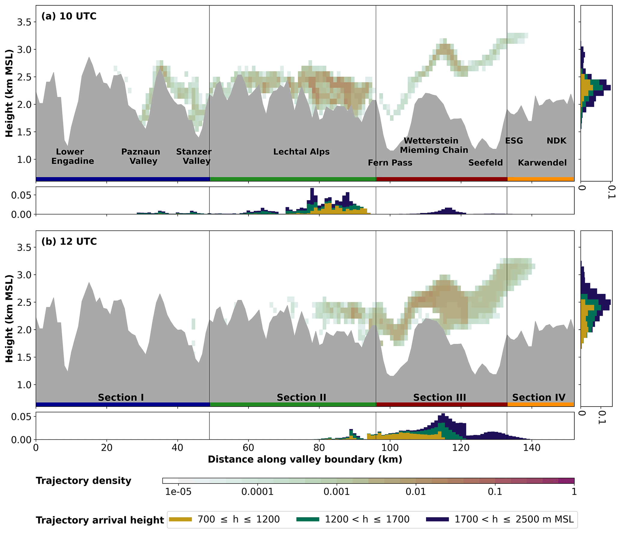
Figure 11 Density of trajectories crossing the Inn Valley boundary (see line IVB in Fig. 1b) through various different sections. Shown is the density on transect IVB for trajectories arriving in Innsbruck at (a) 10:00 UTC and (b) 12:00 UTC on 29 October 2017. Color contours indicate the fraction of all trajectories passing through a vertical rectangle with 1 km width and 100 m height. The histogram in the lower panel (right panel) shows the horizontal (vertical) distribution of the trajectory density summed up in vertical (horizontal) direction. The three stacked bars in the histogram correspond to the fraction of trajectories arriving in Innsbruck in the three layers: 700 to 1200, 1200 to 1700, and 1700 to 2500 m a.m.s.l., respectively (see legend). Four subsections of the transect as described in Sect. 2.3.2 are indicated by horizontal color bars and are separated by vertical black lines. Important terrain features are named in (a).

A minor portion of trajectories enters the Inn Valley further west in the region of the Arlberg and Silvretta passes via the Stanzer and Paznaun valleys through section I (Fig. 11a). Their contribution is only about 10 % at 10:00 UTC (Fig. 10e). Trajectories entering this way are already below the surrounding crest height as they cross the valley boundary (Fig. 11a). For earlier times some trajectories even enter the Inn Valley through the Lower Engadine (not shown). It is noteworthy that the southern trajectory branch originating from Switzerland makes a comparatively large contribution of about 40 % to trajectories entering via section I (not shown).

A tiny part of less than 1 % crosses IVB at 10:00 UTC through section III (Fig. 10e), which represents the Wetterstein Mountains and the Mieming Chain (Fig. 11a). A negligible part passes through the most western part of section IV which represents the Erlspitze Group of the Karwendel. The crossing takes place in a narrow filament located between about 2500 and 3500 m a.m.s.l. (Fig. 11a). A possible explanation for the shape of this filament is in the alignment of trajectories with IVB in this region. With the trajectories almost parallel to IVB in this part the vertical evolution of the flow with the lifting on the windward sides of the Wetterstein Mountains and the Karwendel is reflected in the shape of the crossing pattern.

At 10:00 UTC, the four sections contribute differently to the distribution of trajectory arrival heights. Trajectories crossing the Lechtal Alps within the main cluster end up distributed over the whole valley atmosphere (lower histogram in Fig. 11a). In contrast, most trajectories passing through section I reach Innsbruck mainly in the mid and upper valley atmosphere. Trajectories crossing through the aforementioned filament in sections III and IV only reach Innsbruck in the upper valley atmosphere above 1700 m a.m.s.l. In summary, only trajectories passing the Lechtal Alps end up in the lower valley atmosphere at this time.

After 10:00 UTC a strong change in the patterns of the valley boundary crossing can be identified (Fig. 10e). Between 10:00 and 12:00 UTC the contribution through section III (Wetterstein Mountains and Mieming Chain) increases from zero to more than 80 %, while the contribution through section II (Lechtal Alps) decreases to less than 20 %. After this pattern change almost no trajectory enters through section I, while the contribution through section IV (Karwendel) increases from zero to a few percent at the very end of the event (Fig. 10e).

The majority of trajectories entering at 12:00 UTC through section II still cross the valley boundary mainly in the northeastern part of the Lechtal Alps below 2500 m a.m.s.l. and still arrive in Innsbruck distributed over the whole valley atmosphere. However, the crossing through section III dominates now (Fig. 11b). The terrain-following structure of the trajectory plume in sections III and IV is similar to that at 10:00 UTC. At this time, however, the plume is located at a slightly lower height and has a broader vertical extent (Fig. 11b). For the trajectories entering through sections III and IV a strong dependency between the crossing position, the crossing height, and the arrival height can be observed (Fig. 11b). Here the distributions of the crossing positions for the trajectories arriving in Innsbruck at higher levels are shifted towards positions further east and towards higher levels on the valley boundary line IVB.

5.2 Penetration mechanisms

In the previous section a drastic temporal change was identified in where and how the air passes IVB. In the second half of the event the major part of the trajectories enter the Inn Valley closer to Innsbruck. The main objective of the following sections is to explore the dominating penetration mechanisms and the diabatic processes on the leeward side before and after that pattern shift.

5.2.1 Lechtal Alps

Until 10:00 UTC the vast majority of trajectories enters the Inn Valley via section II over the Lechtal Alps (Figs. 10e and 11a). These trajectories stay close to the terrain at about 2000 m a.m.s.l. before they enter the Inn Valley (Fig. 12a). They are trapped near crest height in an about 500 m deep layer of high stability. In this phase trajectories of different arrival heights stay initially close together over the high terrain. In the lee of the Lechtal Alps the trajectories descend in a gravity wave below crest height (Fig. 12a) and get deflected and channeled by the Inn Valley (Fig. 12c). Some of the trajectories already descend down to the valley floor directly on the northern slope of the Inn Valley (not shown), but the majority stays in the upper valley atmosphere just below crest height.

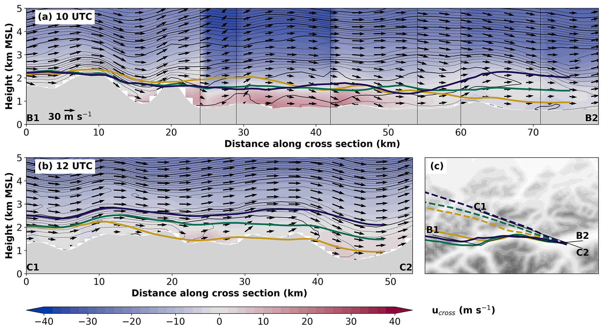
Figure 12 Vertical transect of equivalent potential temperature and wind along (a) CS_LTA at 10:00 UTC and (b) CS_WST at 12:00 UTC on 29 October 2017 and median trajectory height selected by the arrival height in Innsbruck and the dominant section where the trajectories cross the Inn Valley boundary. Black contour lines and wind vectors are as in Fig. 5. Color contours represent horizontal wind component perpendicular to the transect (positive into the plain). Discontinuities in (a) are caused by kinks in the transect (see alignment in c). Lines indicate median trajectory height projected to the transect for trajectories crossing section II in (a) and section III in (b). Line colors indicate the trajectory arrival heights as in Fig. 11. Topographic map in (c) with median trajectory position for trajectories arriving via section II at 10:00 UTC (thick solid lines) and section III at 12:00 UTC (thick dashed lines). Thin black lines indicate the location of the cross sections, and text labels illustrate the start and end points of the transects.

As seen in Sect. 3 a rotor covering the whole valley atmosphere is dominating the flow field in this region of the Inn Valley. This can also be seen in Fig. 12a between x=25 and 55 km by a local minimum of θ_e at heights around 1500 m a.m.s.l. and strong cross-valley winds with positive (negative) values below (above) 1500 m a.m.s.l. As the cross-valley rotor circulation is superimposed by a westerly along-valley flow (see Fig. 3 and along-valley component in Fig. 12a), this results in a helix-shaped flow pattern which leads to the helix shape of the three different mean trajectories in Fig. 12a. Until the region of Zirl (see Fig. 3 and x=55 km in Fig. 12a) the trajectories are located within this rotor with the median trajectory height for all arrival heights located in the center of the rotor at about 1500 m a.m.s.l. In the region of Zirl, where the Inn Valley changes its orientation, the trajectories of different arrival heights are quickly separated vertically from each other. This could at least partly be caused by trajectories impinging on the southern foothills of the Karwendel (see hill in Fig. 12a at around x=63 km) and by a hydraulic jump in the lee of the northern Stubai Alps south of the Inn Valley (not shown).

5.2.2 Wetterstein Mountains, Mieming Chain, and Karwendel

After 10:00 UTC a shift in the penetration pattern takes place with the majority of trajectories now crossing the valley boundary in section III (Fig. 10e). However, especially for the trajectories arriving in Innsbruck in the mid and upper valley atmosphere, a clear distinction between a penetration in the lee of the Wetterstein Mountains and Mieming Chain (section III) and the Karwendel (section IV) is not possible as the trajectories flow almost parallel to the line IVB in this region (see Figs. 1b and 12c). As shown in Fig. 12b, these trajectories pass first the Wetterstein Mountains and Mieming Chain on average between 2000 and 2500 m a.m.s.l. Afterwards they stay above crest height nearly parallel to the crest line (Fig. 12c) until they finally penetrate into the Inn Valley in the lee of the most western part of the Karwendel (Erlspitze Group). In contrast, the trajectories reaching Innsbruck in the lower valley atmosphere subside below crest height in the lee of the Mieming Chain but remain on average in the mid valley atmosphere until their final penetration to the valley floor right before arriving in Innsbruck (Fig. 12b). In both cases, the final penetration into the valley is caused by subsidence in a gravity wave. It is noteworthy that in contrast to the situation at 10:00 UTC a clear horizontal and vertical separation between the trajectories arriving at different heights in Innsbruck already occurs with the crossing of the Inn Valley boundary.

5.3 Diabatic processes on the leeward side

5.3.1 Lechtal Alps

The trajectories arriving in Innsbruck at 10:00 UTC pass the Lechtal Alps saturated within the clouds (Fig. 13a, d). Here lifting at the ridge of the Lechtal Alps leads to further formation of hydrometeors and thus to temporary diabatic heating (see low-arriving trajectories, Fig. 13a–c), while the continuous increase in θ_il illustrates an irreversible warming due to orographic precipitation and the associated moisture loss (Fig. 13b, c). Subsidence in the lee of the Lechtal Alps finally leads to drying of the air and diabatic cooling due to the evaporation of hydrometeors (Fig. 13a–d). Once the trajectories are deflected in the valley's direction, they stay within the rotor circulation. Here, the trajectories remain on average in the slightly subsaturated air below the cloud base with no substantial moisture changes taking place (Fig. 13a, c, d). After the vertical separation of the trajectories at about 15 km before the arrival in Innsbruck, only the fraction of the trajectories arriving in the upper valley atmosphere gets lifted into the cloud again, leading to diabatic warming and the associated formation of hydrometeors and subsequent moisture loss.

Figure 13 Vertical transect of the wind field and the median trajectory height are as in Fig. 12 for (a) CS_LTA at 10:00 UTC and (e) CS_WST at 12:00 UTC on 29 October 2017. The black contour line indicates a relative humidity of 99 %. Color contours represent the total hydrometeor mixing ratio q_t–q_v. Panels (b)–(d) and (f)–(h) show median trajectory properties for the three arrival heights (same line colors as in Fig. 11). (b, f) θ (solid line) and θ_il (dashed line); (c, g) q_v (solid line) and q_t (dashed line); and (d, h) relative humidity.

5.3.2 Wetterstein Mountains, Mieming Chain, and Karwendel

The trajectories arriving in Innsbruck at 12:00 UTC also pass the mountains within the clouds (Fig. 13e). Here, lifting upstream of the Wetterstein Mountains and Mieming Chain leads to the formation of more hydrometeors and consequently to diabatic heating (Fig. 13e–g at about x=10 km). The same process is taking place for the trajectories arriving in the upper valley atmosphere upstream of the Karwendel (x=30 km in Fig. 13e–g). The low-arriving trajectories descend below the cloud base already with their subsidence to the mid valley atmosphere in the lee of the Mieming Chain and stay subsaturated until their arrival in Innsbruck (Fig. 13e, h after about x=15 km). Staying within the clouds, moisture loss due to precipitation falling out (Fig. 13g) leads to continuous irreversible diabatic heating for the mid- and high-arriving trajectories, illustrated by the increase in θ_il in Fig. 13f. Finally, subsidence in the gravity wave in the lee of the Karwendel leads to drying, while parts of the hydrometeors get advected into subsaturated air (Fig. 13e). Here, the trajectories arriving in the mid valley atmosphere become subsaturated about 5 km before arriving in Innsbruck, while the ones arriving in the upper levels stay in the clouds until the end.

6 Discussion

6.1 Flow patterns and diabatic processes on the upstream side

Up to now diabatic processes on the windward side have not been studied for north or west foehn. However, the results of this study are comparable to flow patterns south of the Alps in the context of south foehn. Like in our case, the importance of different flow branches that contribute to the foehn air arriving at the target location has been shown for south foehn, for example, by Miltenberger et al. (2016) or Jansing and Sprenger (2020). In agreement with Miltenberger et al. (2016) the change in the contributions from different flow branches was connected to changes in the diabatic processes along the pathway. However, exploring the reason for this changing flow branch contribution is beyond the scope of this study. With pronounced orographic lifting and associated precipitation on the windward side this event has similarities to the so-called Swiss-type foehn studied by Würsch and Sprenger (2015) or the moist case of Miltenberger et al. (2016). The associated moisture loss and the net diabatic heating in our study are in the same range as described in Würsch and Sprenger (2015). The gradual descent of the trajectories' height far upstream of the Alps, together with the decreasing stability of the impinging air mass in our case, can be interpreted as a transition from a “flow around” into a “flow over” regime. The observed increasing moisture loss and diabatic heating are in agreement with the interpretation of a positive feedback between lifting, moisture loss, and diabatic heating in Buzzi et al. (1998).

The effect of trajectory scrambling as described in Miltenberger et al. (2016) could not be found in our case. Miltenberger et al. (2016) found a vertical separation of the trajectories downstream of the main Alpine crest depending on the diabatic temperature evolution. In their case, trajectories starting at lower levels on the windward side experienced a loss of moisture, a net diabatic heating, and ended up at higher levels on the downstream side and vice versa. In contrast, in our case the majority of trajectories with a net moisture loss and the minority of trajectories with a net moisture uptake both ended up on average at a similar height within the valley atmosphere.

6.2 Penetration into the Inn Valley

Our results partly confirm previous findings on north foehn in the Inn Valley. In agreement with Zängl (2006), the penetration into the Inn Valley took place via several different pathways covering the entire region west of Innsbruck. Zängl (2006) suggested an increasing contribution of the Arlberg region with a stronger westerly component of the large-scale flow or with the presence of a barrier jet in the Alpine foreland. This partly agrees with the high contribution of the southern air stream from Switzerland to the trajectories penetrating via section I in this study. However, a simple direct relation does not seem to exist given the fact that the contribution of the trajectories from Switzerland increased towards the end of the foehn event, although almost none of them passed through section I (see Fig. 10d and e). In other words, the trajectory origin does not necessarily determine the region where the trajectories enter the Inn Valley.

In agreement with Zängl (2006), we identified gravity waves in the lee of the Lechtal Alps as one important mechanism for the air to penetrate into the Inn Valley. However, we also found an additional mechanism that has not been mentioned before which is a persistent cross-valley rotor circulation in the Inn Valley. The penetration associated with this rotor resembles scenario D in Strauss et al. (2016) with a large atmospheric rotor covering the whole valley atmosphere underneath a trapped lee wave. The subsidence on the downstream side of the rotor (which is the windward side of the subsequent mountain ridge) provides an effective mechanism to import air into the valley atmosphere. The decreasing stability and increasing wind speed above 2500 m a.m.s.l. (Fig. 4a) result in a vertically decreasing Scorer parameter (Scorer, 1949) and thus provide an environment favorable for the formation of such trapped lee waves (Lin, 2007). The rotor therefore resembles a type I rotor according to Hertenstein and Kuettner (2005). Downstream topography has been shown to impact the lee wave pattern through wave interference (Grubišić and Stiperski, 2009; Stiperski and Grubišić, 2011). Such downstream topography is in our case, for example, the mountain range of the Stubai Alps south of the Inn Valley, as well as the ridge between Tschirgant and Simmering northwest of Haiming (see Fig. 3 and hill around x=20 km in Fig. 12a). Given the fact that no rotor formed in the slightly wider part of the Inn Valley east of Innsbruck (Figs. 3, 12b), the rotor formation appears to be strongly dependent on the valley geometry.

Similar to Strauss et al. (2016), the position and strength of the rotor depended on the associated gravity wave field aloft. From 10:00 to 12:00 UTC the horizontal wavelength and the amplitude of the trapped lee wave increased (Fig. 4b). This resulted in stronger subsidence on the northern slope of the Inn Valley and a downstream shift of the rotor position which weakened the rotor-induced subsidence and the associated penetration mechanism. A possible reason for this change in the wave pattern could be the weakening of the crest-level stability (which is consistent with the weakening of the upstream stability discussed in Sect. 4.3) and a slight increase in crest-level wind speed (see Figs. 4b and 5b, around 2500 m a.m.s.l.). In Xue et al. (2020) a weakening of the upstream stratification, together with reduced upstream blocking, and a strengthening of the cross-mountain winds led to a widening and an amplification of the lee wave. Similarly, in Strauss et al. (2016) increased crest-level wind speeds led to an increase in the horizontal wavelength and the wave amplitude, which resulted in a downstream shift of the rotor position and the strongest wind speeds at the valley floor. Apart from the changes in the upstream stratification, a slight shift in the crest-level wind direction may have led to changes in the effective distance to the downstream topography resulting in a changed interference pattern (Grubišić and Stiperski, 2009; Stiperski and Grubišić, 2011). Additionally, this shift to a slightly stronger northerly wind component presumably facilitated the penetration in the lee of the Wetterstein Mountains and Mieming Chain given the east–west orientation of the Inn Valley in this area. Hence, the lee wave pattern and thus also the rotor and its associated penetration pattern are very sensitive to subtle changes in the upstream and crest-level flow conditions.

Our results disagree with those of Zängl (2006) for the air penetrating into the Inn Valley in the lee of the most western part of the Karwendel in the second phase of the event. Zängl (2006) argued that in his case the northerly flow in the lee of this mountain ridge resulted from deflection of the down valley flow by a local terrain corrugation. However, in our case the trajectories passing the Karwendel did not originate from inside but rather from far north of the Inn Valley (Fig. 12c). Moreover, the final penetration of air into the valley was partly caused by a gravity wave in the lee of the Karwendel which was not present in the case of Zängl (2006). The pathway through the terrain gap of Seefeld as suggested in Haas (2006) did not play a role for the air mass penetration in our case. Our results illustrate that the locations and mechanisms of the penetration are strongly time- and case-dependent. Furthermore, they can only be convincingly determined by combining Lagrangian and Eulerian perspectives.

In contrast to Zängl (2006), orographic precipitation did not suppress the evolution and breakthrough of foehn in the Inn Valley in our case. Our results are closer to those of Haas (2006), with precipitation being formed upstream and being advected into the Inn Valley, resembling the characteristics of “dimmerfoehn” (Richner and Hächler, 2013). Zängl (2006) reasoned that precipitation falling into layers of unsaturated air in the valley stabilized these layers due to evaporative cooling, leading to a dampening of the amplitude of gravity waves and thus preventing the foehn from penetrating. In our case the air along the trajectories experienced a net diabatic warming while crossing the Alps due to the formation of orographic precipitation. Inside the valley the evaporative cooling from precipitation formed above the air parcel only played a marginal role, and the air inside the valley stayed largely well-mixed.

In our case the change in the upstream flow conditions coincides with the change in the penetration pattern (Fig. 10). Additionally, our results on the valley scale suggest that the pattern change here is a result of rather subtle changes in the flow conditions at crest-height. However, the question of the extent to which the upstream conditions and the penetration mechanisms are connected remains unclear. Hence, it would be interesting to extend this analysis to other cases, especially “dry” events without precipitation upstream since they represent about 60 % of all north foehn cases according to Haas (2006).

6.3 Foehn classification

Due to the channeling of the flow into the valley direction most foehn-like flows originating north of the Alps appear as strong westerly to northwesterly winds in Innsbruck, independent of where the penetration into the valley takes place. Because of that, different authors have used different definitions so that there exists no uniform classification to distinguish between west foehn, northwest foehn, and north foehn. Following the local-scale approaches based on the wind direction in Innsbruck of Trabert (1903) and Wankmüller (1995), the case presented here would have to be called a west foehn (see Fig. 6). One weakness of this approach, however, is that the local wind direction varies strongly along the valley due to changes in the valley orientation. Strictly following their approach, this would result in different classifications for the same event at different locations. Following the larger-scale approaches of Zängl (2006) and Haas (2006), the case would have to be called a north foehn. Arguments for this are the large-scale flow crossing the Alps with a northerly component above crest height and northerly flow in the Wipp Valley.

However, the trajectory analysis conducted in this study provides the possibility for two new classification approaches based on a Lagrangian perspective on (1) the large-scale air mass origin and (2) the point of penetration into the Inn Valley. With the first approach, which is an Alpine-scale perspective, one finds that the major part of the trajectories originates north of Innsbruck (Fig. 10d), more specifically in the northwestern quadrant (Fig. 7). A clear limitation of this approach is the subjectivity of the choices of how long the trajectories are calculated backwards in time and how the individual sectors are defined. For the second approach, which is a valley-scale perspective, the valley boundary and individual sections have to be defined. In our case, section I has a south–north orientation and section II a southwest–northeast orientation. Hence, even for a pure westerly flow not only section I but also section II could be crossed leading to a possible penetration through these sections. Hence, flow conditions that lead to a dominant flow through sections I and II could be classified as west foehn from a valley-scale perspective. Likewise, a dominant flow through section III could be called northwest foehn and a dominant flow through section IV north foehn. A limitation of this approach is that this is only valid for Innsbruck as trajectories released from different locations along the Inn Valley will presumably experience different contributions. Based on these two approaches the foehn in this study could be classified as a northwest foehn on an Alpine scale throughout the whole event, while on the valley scale a gradual transition from a west foehn to a northwest foehn is more appropriate.

Apart from the specific limitations of the two new approaches presented above, a trajectory-based classification would have other more general limitations. Turbulent processes may not be sufficiently captured by the model and are not represented in the trajectory calculation, resulting most likely in an underestimation of the trajectory dispersion. Furthermore, a trajectory analysis is typically not available on an operational basis, which excludes its use for real-time foehn diagnosis and forecasting. Last but not least, a “binary” classification in one or the other category remains subjective and is not able to reflect the variety of penetration mechanisms and their transient contributions.

7 Conclusions

In this study the foehn event of PIANO IOP 1 on 29 October 2017 was investigated based on a mesoscale numerical simulation, backward trajectories, and observations. The aim was to determine the origin, the pathways, and the entrance regions of the air mass penetrating into the Inn Valley and finally arriving in Innsbruck. Furthermore, diabatic air mass transformation processes from the windward to the leeward side over various mountain ridges were assessed. Concerning the foehn event in general and the performance of the WRF simulations the most important results are as follows:

• The main phase of the foehn event lasted from the morning to the afternoon of 29 October 2017 with the foehn breakthrough at the valley floor in Innsbruck at about 08:00 UTC and the foehn breakdown at 15:30 UTC when a cold front arrived. During the foehn period the strong northwesterly flow above crest height was channeled into the valley direction and appeared as a strong westerly wind in Innsbruck. Orographic precipitation occurred especially on the northern slopes of the Alps but was also observed in the Inn Valley.

• On the Alpine scale the WRF simulation was able to reproduce the regional flow patterns of low-level deflection and upper-level crossing, as well as the pattern of orographic precipitation. On the valley scale the model underestimated the strength of the nighttime cold pool and the associated decoupling of the valley atmosphere from the flow aloft. Consequently, the flow in the valley was too strong and the foehn breakthrough at the valley floor occurred too early. However, once the foehn was fully established also in reality, the simulated flow field agreed reasonably well with the observations, apart from a cold model bias of 3 to 4 K in the lowest 1000 m a.g.l.

On the Alpine scale the main findings of the trajectory analysis are as follows:

• Backward trajectories calculated over the duration of 6 h revealed the location of the air mass origin in the northwest of the Inn Valley with two pronounced air steams. The main (northern) air stream originated in France, crossed the mountain ranges of the Vosges and the Black Forest, and finally reached the Alps in the region of Lake Constance and the Rhine Valley. This air stream contributed 60 % to 90 % of the foehn air arriving in Innsbruck. The secondary (southern) air stream originated over the Swiss Plateau and was aligned parallel to the Alpine rim until it finally impinged on the Alps in the same region as the main branch. During the event the contributions of the two air streams slightly changed with a maximum contribution from the northern branch of about 90 % between 11:00 and 13:00 UTC. With the main part of the trajectories coming from the northwestern sector, the foehn event could be classified on an Alpine scale as a northwest foehn.

• For the trajectories of the main air stream, orographic precipitation over the Vosges, the Black Forest, and the Alps led to moisture loss of about 1 g kg⁻¹ and net diabatic heating of about 2.5 K. In contrast, trajectories of the southern flow branch experienced moisture uptake and diabatic cooling on the windward (west) side of the Alps most likely due to evaporation of precipitation from aloft. Nevertheless, subsequent diabatic heating over the Alps dominated the total heating also for the southern branch and led to a net increase in potential temperature of about 2 K along the trajectories. This increase is most likely attributed to orographic precipitation over the Alps. However, the role of other heating processes such as turbulence and the role of three-dimensional moisture exchange could not be conclusively determined.

On the valley scale the main findings of the trajectory analysis are as follows:

• The entrance region, where the main part of the air mass penetrated into the Inn Valley, changed over the course of the event. Until 10:00 UTC the majority of the trajectories (80 % to 90 %) entered the Inn Valley via the Lechtal Alps, while the remaining part largely entered the Inn Valley further to the west in the Arlberg region. After 12:00 UTC the dominant part (70 % to 85 %) entered via the Wetterstein Mountains and Mieming Chain. A minor part entered via the most western part of the Karwendel. Penetration of air into the Inn Valley directly from the north of Innsbruck via the Nordkette was negligible at all times. From a Lagrangian-based valley-scale perspective the shift in the penetration pattern between 10:00 and 12:00 UTC can be interpreted as a transition from west to northwest foehn.

• For the trajectories entering the valley via the Lechtal Alps two penetration mechanisms were important. A gravity wave in the lee of the Lechtal Alps forced the trajectories below crest height and for a smaller fraction allowed a penetration all the way to the valley floor. For the majority of trajectories, however, a rotor underneath this lee wave stretching over a distance of about 30 km played a crucial role in bringing the trajectories into the valley atmosphere. For the trajectories entering the valley closer to Innsbruck the penetration was associated with a gravity wave in the lee of the Wetterstein Mountains and Mieming Chain, as well as in the lee of the most western part of the Karwendel.

• A weakening of the upstream stability and an increase in crest-level wind speeds, together with a slight shift to a stronger northerly component, likely led to a widening and an amplification of the lee waves over the Inn Valley in the second phase of the event. This resulted in stronger subsidence on the northern slopes of the Inn Valley and a weakening of the rotor-induced penetration. Apart from that, the shift in wind direction likely facilitated the penetration in the lee of the Wetterstein Mountains and Mieming Chain given the change in the orientation of the Inn Valley in this region.

The study showed the important role of diabatic processes on the temperature changes along the trajectories. With the methods used here, however, only a qualitative assessment of individual processes was possible. This gap could be filled by retrieving and analyzing individual temperature tendencies from individual microphysical, turbulent, and radiative processes along the trajectories in order to close the budgets of heat and moisture. This could be achieved either by using online trajectories, calculated already within the numerical model (e.g., Miltenberger et al., 2016), or by retrieving the tendency terms (e.g., Göbel et al., 2022; Umek et al., 2021) and using them in offline trajectories similar to the investigations done here. One limitation of this study is the neglect of turbulent effects on trajectory dispersion. This could be improved either by substantially increasing model resolution or by using trajectory tools that at least account for parameterized turbulence. However, which of these approaches is more practical and fruitful remains to be shown. Furthermore, it has to be shown to what extent a higher model grid resolution for a better representation of stratification and turbulence in the valley atmosphere (Umek et al., 2022) also improves the trajectory dispersion in the mountain boundary layer. Finally, the analysis should be extended to other cases, especially to dry events without precipitation in which different types of processes may dominate.