Sudden stratospheric warmings during El Niño and La Niña: sensitivity to atmospheric model biases

The number of sudden stratospheric warmings (SSWs) per year is affected by the phase of the El Niño–Southern Oscillation (ENSO), yet there are discrepancies between the observed and modelled relationship. We investigate how systematic model biases in atmospheric winds and temperatures may affect the ENSO–SSW connection. A two-step bias correction process is applied to the troposphere, stratosphere, or full atmosphere of an atmospheric general circulation model. ENSO-type sensitivity experiments are then performed by adding El Niño and La Niña sea surface temperature (SST) anomalies to the model's prescribed SSTs, to reveal the impact of differing climatologies on the ENSO–SSW teleconnection.

The number of SSWs per year is overestimated in the control run, and this statistic is improved when biases are reduced in both the stratosphere and troposphere. The seasonal cycle of SSWs is also improved by the bias corrections. The composite SSW responses in the stratospheric zonal wind, geopotential height, and surface response are well represented in both the control and bias-corrected runs. The model response of SSWs to ENSO phase is more linear than in observations, in line with previous modelling studies, and this is not changed by the reduced biases. However, the ratio of wave 1 events to wave 2 events as well as the tendency to have more wave 1 events during El Niño years than La Niña years is improved in the bias-corrected runs.

1 Introduction

The El Niño–Southern Oscillation (ENSO) can impact the Northern Hemisphere wintertime stratospheric variability, and the prevalence of sudden stratospheric warmings (SSWs). Understanding the ENSO–SSW link can help interpret seasonal model predictions and improve seasonal forecasts. The increased convection in the tropical east Pacific during an El Niño event triggers a Rossby wave train that strengthens and deepens the Aleutian low (Bell et al., 2009; Cagnazzo and Manzini, 2009). This leads to constructive linear interference of the planetary waves and an increased wave flux into the stratosphere and hence a weakened stratospheric polar vortex. During El Niño years the polar vortex is, on average, weaker than in neutral years, and El Niño is also associated with an increase in the number of SSWs (Domeisen et al., 2019).

Although La Niña is the opposite phase to El Niño, the negative SST anomalies tend to be weaker, more westward, and have a different time evolution (Hoerling et al., 1997; Larkin and Harrison, 2002; Frauen et al., 2014). The decrease in convection in the topical east Pacific associated with La Niña still leads to a shallower Aleutian low, decreased wave flux, and a stronger polar vortex (Iza et al., 2016; Jiménez-Esteve and Domeisen, 2019; Domeisen et al., 2019). The anomalous La Niña response is weaker than El Niño due in part to the weaker response of the tropical convection and Rossby wave forcing (Trascasa-Castro et al., 2019). The changes to the vertical wave activity flux seem a valid dynamical argument as to why El Niño might lead to more SSWs and La Niña might lead to fewer SSWs; however, the observational record is not so clear. There is a higher chance of an SSW during El Niño years, but there is also an increase in SSW frequency associated with La Niña years (Butler et al., 2014). However, there may be sampling errors due to the relatively short observational record (Domeisen et al., 2019), and the La Niña–SSW relationship is sensitive to the SSW definition (Song and Son, 2018). Modelling studies show the increased likelihood of an SSW during El Niño and show a decreased likelihood of SSWs during La Niña years (Polvani et al., 2017; Song and Son, 2018). It is unclear if the discrepancy between models and observations is due to the low number of observed ENSO and SSW events in observations or non-linearities in the ENSO teleconnections which the models are unable to simulate (Domeisen et al., 2019).

The role of mean state model biases has been investigated for some aspects of the ENSO–SSW teleconnection. Biases in the tropical Pacific SSTs can lead to different ENSO dynamics (Bayr et al., 2018) and affect the position of the North Pacific sea level pressure response (Bayr et al., 2019). Mean state biases in the extratropical circulation can affect the propagation of Rossby waves (Li et al., 2020) and their impact on North Pacific SSTs (Dawson et al., 2011). The impact of climatological biases on the mean ENSO-to-Northern Hemisphere teleconnection was discussed in Tyrrell and Karpechko (2021), using output from the same modelling experiments as in this paper (see Sect. 2). It was found that mean state of the Aleutian low changed the response of the polar vortex to an El Niño forcing by modulating the upward wave flux to the stratosphere. Biases in the strength of the polar vortex did not impact its anomalous response to ENSO, and the North Atlantic Oscillation (NAO) response was not impacted by biases.

In this paper we investigate how the climatological biases in atmospheric winds and temperatures affect the relationship between ENSO and Northern Hemisphere SSWs. We use a bias correction technique to reduce atmospheric biases at specific levels to create different climates, within which we can run ENSO-like SST perturbation experiments. The bias correction technique and data are described in Sect. 2; in Sect. 3 we present the bias reductions and mean ENSO response (Sect. 3.1); the statistics of SSWs (Sect. 3.2), downward propagation, and the surface response (Sect. 3.3); and the heat flux response (Sect. 3.4). A discussion and conclusions are presented in Sect. 4.

2 Data and methods

2.1 Bias corrections

We used the ECHAM6 atmospheric model (Stevens et al., 2013), with a horizontal truncation of T63 and 95 levels in the vertical with a model top at 0.02 hPa. It was run in bias-corrected and biased modes and with SST perturbation experiments. The bias correction process follows Kharin and Scinocca (2012) and has been used to study the effects of model biases on the Eurasian snow extent–polar vortex connection (Tyrrell et al., 2020), Quasi-Biennial Oscillation teleconnections (Karpechko et al., 2021), and ENSO–Northern Hemisphere winter teleconnections (Tyrrell and Karpechko, 2021) and involves two steps: first, the dynamic variables of the model (divergence, vorticity, temperature, and log of surface pressure) are nudged towards ERA-Interim reanalysis. During this step the nudging tendencies are recorded every 6 h. A total of 40 years of nudging tendencies are then composited and smoothed to create an annual climatology of the nudging tendencies. This climatology represents the inherent biases in the model. In the second step, the nudging tendency climatology is added to the model as an additional tendency at each time step, in order to correct the biases in the model's climatology. For the second step it was experimentally found that the biggest reduction in biases occurred when only the divergence and temperature were corrected. The dynamic variables of ECHAM6 are solved using a spectral decomposition of the globe, which allows for nudging and bias correcting on specific wavenumbers. Wavenumbers below n=21 were nudged and corrected, which means that features below about 1000 km were not corrected. The bias corrections can also be applied at different height levels, and three experiments were performed with bias corrections in the troposphere only, TropBC; stratosphere only, StratBC; and full atmosphere, FullBC (details in Table 1). The critical difference between the nudged and bias-corrected runs is that when the model is nudged it is very tightly constrained towards observations, whereas when the bias correction tendencies are applied the model can still respond realistically to perturbations. Additional details of the bias correction scheme are available in Tyrrell et al. (2020) and Tyrrell and Karpechko (2021).

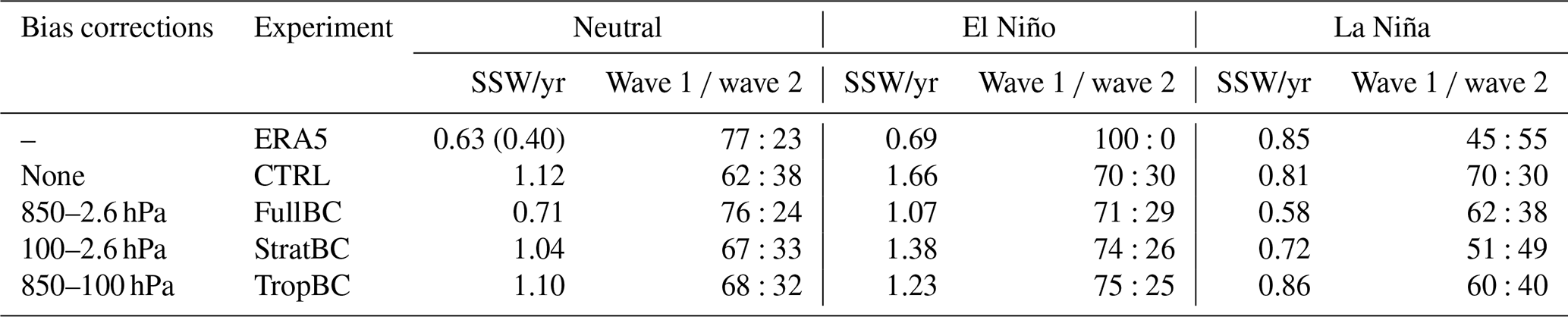
Table 1 Experiment names and details for bias correction and ENSO experiments. Number of SSWs per year calculated from 100 years in the model experiments and 41 years of ERA5 data. For ERA5, the SSW frequency in the third column is shown for all years and only for years with a neutral ENSO in brackets. The wave 1 : wave 2 ratio is based on the heat flux at 100 hPa, 45–75^∘ N.

2.2 El Niño and La Niña experiments

Simplified ENSO SST sensitivity experiments were performed using the bias-corrected climatologies as described in Tyrrell and Karpechko (2021). For the ENSO SST pattern we used a regression of the Niño3.4 time series and HadISST SSTs from 1979–2009. Only the positive regression values between 30^∘ S and 30^∘ N and east of 150^∘ E in the Pacific Ocean were used, and the regression values were multiplied by 1.5 to strengthen the response, corresponding to an El Niño or La Niña forcing magnitude of 1.5 K. There are also ENSO-related SST anomalies outside the tropical Pacific which were excluded from the perturbed SST forcing. Although they can be important for some ENSO teleconnections, they are primarily a response to the tropical Pacific forcing and occur at time lag (Tyrrell et al., 2015), so they were excluded to reduce the complexity of the forced ENSO signal. Climatological SSTs using HadISST data from 1979–2009 were used outside the tropical Pacific and for the control run (CTRL). The ENSO anomaly was kept constant in time (i.e. the anomaly did not vary seasonally), and each experiment was run for 100 years.

The ERA5 data from 1979–2019 (Hersbach et al., 2020) were used as a reference to compare to the model results. El Niño and La Niña years were defined by the DJF value of the Oceanic Niño of ERSST.v5 SST anomalies in the Niño 3.4 region (5^∘ N–5^∘ S, 120–170^∘ W), from the NOAA CPC website (https://origin.cpc.ncep.noaa.gov/products/analysis_monitoring/ensostuff/ONI_v5.php, last access: 16 June 2021), and using a threshold of ±0.5 K; see Supplement Table S1. This results in 13 El Niño years with 9 SSWs, 13 La Niña years with 11 SSWs, and 15 neutral years with 6 SSWs. The relatively low number of El Niño and La Niña years and SSWs means that few of the reanalysis ENSO results have statistical significance, and they may be dependent on the temperature threshold for defining ENSO events. As such, the reanalysis is included as a reference, but a more in-depth analysis focusing on ERA5 – and other observational data sets – would be required to fully verify and explain those results.

The SSW central date is defined using the Charlton–Polvani criterion (Charlton and Polvani, 2007), defined as the first day when zonal mean zonal wind at 60^∘ N and 10 hPa (uz₆₀) is easterly (i.e. uz₆₀<0 m/s). The reversal has to occur during 1 November–31 March. After an SSW has been detected, winds must return to westerlies for 20 consecutive days before another SSW is detected (as in Butler et al., 2017) to avoid multiple detection of the same event, and uz₆₀ must return to westerlies for at least 10 consecutive days before 30 April to exclude final warming.

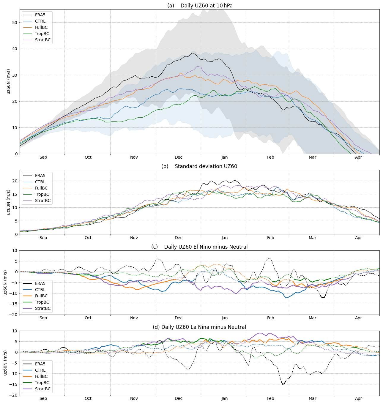
Figure 1 (a) Mean daily zonal mean zonal winds at 60^∘ N and 10 hPa for ERA5 (1979–2019) and control and bias correction experiments (100 years each). Shading shows 1 standard deviation for ERA5 (grey) and CTRL (blue). (b) Mean daily standard deviation for ERA5 and the experiments. (c) Daily uz₆₀ El Niño response calculated as El Niño years minus neutral years, e.g. CTRL_EN – CTRL. (d) Daily uz₆₀ La Niña response calculated as La Niña years minus neutral years. For (c) and (d) the dashed line shows the mean El Niño and La Niña response, and a solid line indicates responses significant at the 5 % level.

3 Results

3.1 Reduced model biases and mean ENSO response

The bias corrections are applied globally at different pressure levels. The reductions in biases have a three-dimensional structure which has relevance to the ENSO teleconnection to the stratospheric vortex and the Northern Hemisphere, and this was explored in Tyrrell and Karpechko (2021). As this paper focuses on SSWs, the reduced model biases in the wintertime polar vortex are of particular interest. In Fig. 1a we show the seasonal progression of uz₆₀ using the mean daily values for the 100-year model runs and 41 years of ERA5 data. The standard deviation for ERA5 and CTRL is also shown as shading. The CTRL run (blue) has a too weak vortex compared to ERA5 from October to January, and this bias is reduced by approximately half in the FullBC and StratBC runs. The bias corrections in TropBC actually increase the bias in the polar vortex in November–December. All model runs effectively capture the polar vortex strength during February and March. As shown in Fig. 1b the interannual variability of the vortex strength is relatively well simulated in CTRL, and the bias corrections do not significantly change the variance. The largest difference between the reanalysis and the model is in January when ERA5 exhibits increased variance, which is not simulated by any of the model runs. The mean difference in daily uz₆₀ between El Niño and neutral years and La Niña and neutral years is shown in Fig. 1c and d for the model (i.e. daily mean of 100 El Niño or La Niña years minus 100 neutral years) and ERA5 (15 El Niño years, 13 La Niña years, minus 13 neutral years). The CTRL, FullBC, and StratBC runs have the strongest mean El Niño response throughout winter, although only the StratBC has a statistically significant response in January (as shown at the 5 % level by bold lines). CTRL and FullBC show a weaker response in January. TropBC has only a weak El Niño response throughout winter. The CTRL has the weakest La Niña response and the StratBC the strongest, with a persistent response from December to March. The mean daily ERA5 response to both El Niño and La Niña shows large variability with little significance in the response. For certain months the ERA5 response is opposite to that seen in the models, e.g. the February–March La Niña response, and at times it shows a similar magnitude and sign, e.g. the La Niña response in January or the El Niño response in March. The mean ENSO response was studied in more detail in Tyrrell and Karpechko (2021), where seasonal mean values indicated that in early winter the models and ERA5 disagreed on sign of the El Niño response and agreed on the La Niña; then in late winter they agreed on the El Niño response and disagreed on La Niña.

Figure 2 Timescales of polar cap (60–90^∘ N area average with cosine weighting) geopotential height (Z_cap) variability. The timescales are defined as days when the autocorrelation function drops to $\mathrm{1}/e$. The time series are smoothed in time with a Gaussian filter (σ=26 d), following Fig. 1 from Baldwin et al. (2003). ERA5 data from 1979–2019, 100 years for each model run (neutral, El Niño, and La Niña).

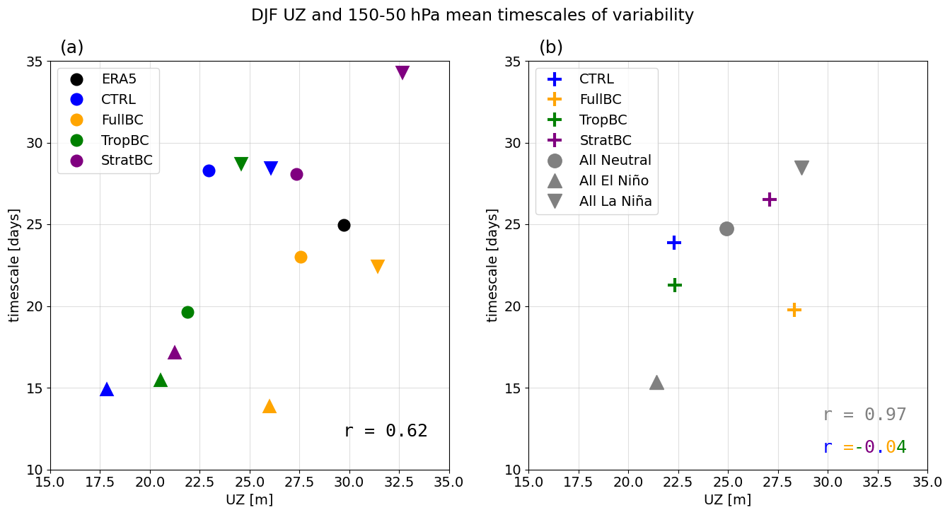
Figure 3 Mean DJF zonal mean zonal wind at 60^∘ N 10 hPa plotted against the weighted average from 50–150 hPa of timescales of polar cap geopotential height (Z_cap) from Fig. 2. (a) Circles are neutral ENSO conditions, upward-pointing triangles are El Niño experiments, and downward-pointing triangles are La Niña experiments. Correlation coefficient for all models and ENSO phases: r=0.62. (b) Coloured crosses show the mean of El Niño, La Niña, and neutral conditions for each experiment (corr. coef.: $r=-\mathrm{0.04}$). The grey circle and triangles show the multi-model mean for each ENSO phase (corr. coef.: r=0.97). ERA5 data from 1979–2019, 100 years for each model run (neutral, El Niño, and La Niña).

Before analysing the SSW responses, we assess the ability of the model to capture the timescales of variability. This is explored in Fig. 2, following Fig. 1 from Baldwin et al. (2003). Using the geopotential height averaged over the polar cap (60–90^∘ N) (Z_cap), and at pressure levels from 1000 to 1 hPa, the figure shows the time in days when the autocorrelation function drops to $\mathrm{1}/e$. The day-to-day variability is smoothed with a Gaussian filter (σ=26 d). The CTRL run captures the timescales of the variability in the winter stratosphere reasonably well, but it is slightly too weak in early winter. The timescales are shorter in the FullBC, and again in TropBC runs, and are slightly longer in StratBC. In all experiments, the timescales are shorter in El Niño experiments and longer in La Niña experiments than in the corresponding neutral experiments. The relationship between the strength of the polar vortex and the timescales of variability was tested in Fig. 3, which plots the DJF UZ 60^∘ N 10 hPa against the DJF timescales of variability averaged from 150 to 50 hPa. Figure 3a shows each ENSO phase for each model separately, so a weaker or stronger vortex strength may be due to the ENSO phase or the bias corrections. A stronger vortex corresponds to longer timescales of variability, and a weaker vortex corresponds to shorter timescales, with a correlation coefficient of r=0.62. We examine this more closely in Fig. 3b by averaging each ENSO phase (i.e. the mean of CTRL_EN, FullBC_EN, TropBC_EN, and StratBC_EN; El Niño is upward-pointing triangles, La Niña is downward-pointing triangles, and neutral is the circles) and each bias-corrected run (i.e. the mean of FullBC, FullBC_EN, FullBC_LN; coloured crosses). We see that as the vortex strengthens and weakens by ENSO phase, the timescales of variability change accordingly. However, changes to the vortex strength due to the bias corrections do not correspond neatly to changes to timescales of variability. A stronger vortex has weaker dynamical variability and is driven by slow radiative processes, which may explain the vortex–variability timescale relationship between ENSO phases. On the other hand, at least in the case of CTRL–FullBC, the relationship does not hold, because FullBC has both stronger vortex and shorter variability; therefore, application of the bias correction technique may have affected the timescales of the variability.

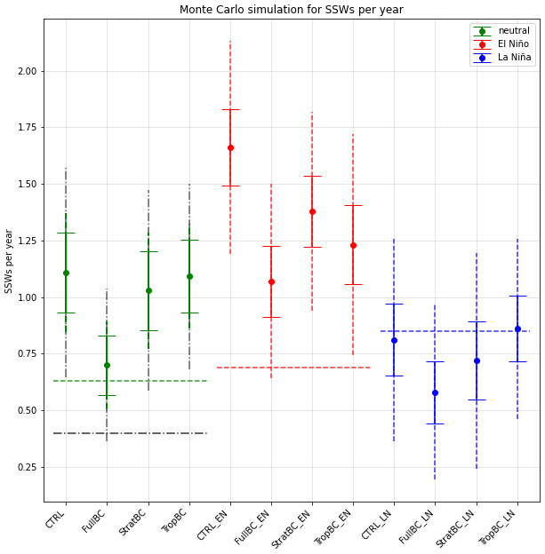
Figure 4 Number of SSWs per year in ECHAM6 and ERA5. The horizontal dashed lines show the ERA5 SSWs per year (green is all 41 years, black dotted–dashed is 15 neutral years, red is 13 El Niño years, blue is 13 La Niña years). Solid error bars show the 5th–95th percentiles for Monte Carlo simulations (N=10 000) choosing 100 random years from each 100-year simulation. Dashed error bars show the 5th–95th percentiles for Monte Carlo simulations where the number of years chosen matches the number of years in ERA5 (green: all 41 years, black dotted–dashed: 15 neutral years, red: 13 El Niño years, blue: 13 La Niña years).

3.2 SSW statistics

The statistics of SSWs are detailed in Table 1 and Fig. 4. The years used for compositing ERA5 are shown in Supplement Table S1. The number of SSWs per year is overestimated in CTRL (1.12 SSWs per year) in comparison to ERA5 (0.63 SSWs per year). This statistic is made more realistic in FullBC (0.71 SSWs per year), but there is only a small improvement in the StratBC (1.04 SSWs per year) and TropBC (1.10 SSWs per year) runs. The significance of the change in the number of SSWs due to the bias corrections was tested using a Monte Carlo simulation (Fig. 4). Specifically, in each experiment, 100 years were randomly chosen with replacement, and the number of SSWs in the sample was calculated. The procedure was repeated 10 000 times to obtain a distribution. The 5–95th percentiles of the distributions are shown in Fig. 4 with solid error bars. We see that FullBC is significantly different from CTRL for neutral (green markers) and El Niño years (red markers), while TropBC differs only for El Niño years. The StratBC runs do not differ significantly from the CTRL for any ENSO phase, although in all cases its distributions lie between those of CTRL and FullBC.

The difference between the models and ERA5 was also tested with Monte Carlo simulations. This was done by choosing the same number of years from the model experiments as there were in the corresponding ERA5 samples. For example, 13 years were taken from the El Niño experiments to match the number of El Niño years in ERA5. The 5–95th percentiles from those simulations are also shown in Fig. 4 as the dashed vertical lines that extend beyond the solid error bars (since there is greater uncertainty with fewer chosen years). The ERA5 statistics are shown as dashed horizontal lines. Two lines are shown to compare the experiments without an ENSO forcing with ERA5. The green dashed line is the number of SSWs per year for the full ERA5 period (41 years), and the black dotted–dashed line is for the 15 neutral years. Although the full period includes El Niño and La Niña years, it is not dependant on one phase and includes a large number of years, whereas the neutral-only years have a small sample size. The model distribution is again estimated by choosing either 41 years (green dashed vertical line which corresponds to the green dashed horizontal line) or 15 years (black dotted–dashed vertical line which corresponds to the black dotted–dashed horizontal line). The results show that FullBC is the only run that consistently captures the SSW statistics of ERA5 in all experiments. Note all La Niña experiments are consistent with ERA5 as well as with each other.

Consistent with previous modelling studies (e.g. Polvani et al., 2017), SSW frequency is increased during El Niño years and decreased during La Niña years in all model experiments. For all model experiments, except TropBC, the number of SSWs during El Niño years is nearly twice as large as that during La Niña years. In TropBC, the exceedance is 40 %. For ERA5 we find that SSW frequency is increased during both El Niño (0.69 SSWs per year) and La Niña (0.85 SSWs per year) years, consistent with previous studies. The years used for compositing ERA5 are shown in Supplement Table S1.

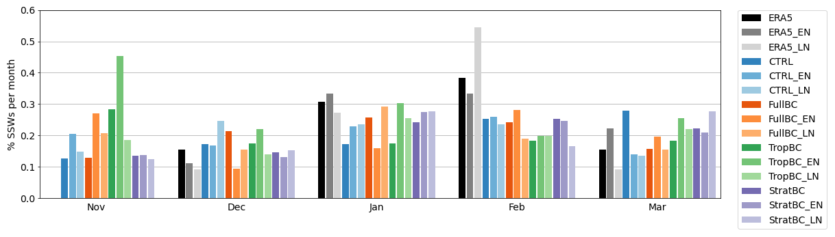
Figure 5 Monthly distribution of SSW frequencies for neutral, El Niño, and La Niña years. The bars are normalized by dividing the number of SSWs in each month by the total number of SSWs for each experiment. ERA5 data from 1979–2019, 100 years for each model run (neutral, El Niño, and La Niña).

The seasonal evolution of SSW frequency is shown in Fig. 5. To explore the differences in seasonal evolution more clearly, the number of SSWs in each month is divided by the total number of SSWs for each experiment, similarly for ERA5. This gives the percentage of the annual total SSWs in each month. Compared to ERA5 there is not enough seasonal variation in CTRL, with too many SSWs in November and March and too few in January and February. The seasonal variation is improved slightly in FullBC, although the seasonal cycle is still underestimated. In StratBC and TropBC the SSW seasonal statistics are not improved as much as in FullBC. In particular, TropBC almost has an inverse of the seasonal relationship of SSWs compared to ERA5, with the most SSWs in November. There are no consistent changes to the seasonality of SSWs with El Niño or La Niña years in the model or ERA5. Note that the model does not have a seasonally evolving ENSO pattern, which may affect the seasonality of SSWs in the ENSO experiments but not in experiments with neutral ENSO conditions which have seasonally evolving SSTs. Yet the neutral ENSO experiments similarly lack seasonal SSW variations.

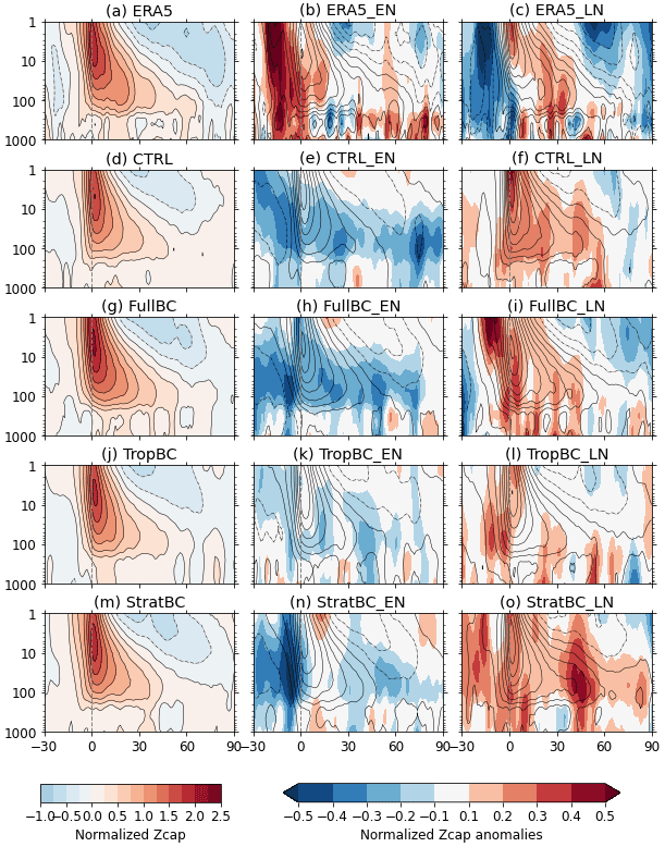
Figure 6 SSW response of normalized polar cap (60–90^∘ N) geopotential height, composited around SSW day zero (shown as a dashed vertical grey line). The left column shows neutral years for the experiments and all years for ERA5. The middle column shows the SSW response in El Niño years with contours (negative values dashed) and the El Niño anomalous SSW response in colours (normalized polar cap geopotential height in El Niño years minus neutral years). The right column is the same for La Niña. ERA5 data from 1979–2019, 100 years for each model run (neutral, El Niño, and La Niña).

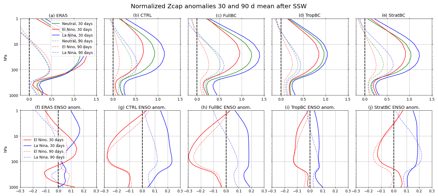
Figure 7 The top row shows normalized polar cap (60–90^∘ N) geopotential height, composited around day zero of and time-averaged for 30 and 90 d after SSWs, for neutral years (green), El Niño years (red), and La Niña years (blue). The bottom row shows the change in the mean Z_cap SSW difference from neutral years due to El Niño (red) and La Niña (blue).

3.3 SSW downward propagation and surface response

Figure 6 shows the SSW composite of normalized Z_cap and then the anomalous values in El Niño an La Niña years relative to neutral years. For ERA5 the ENSO phases are normalized using the standard deviation for all ERA5 years. The CTRL run simulates the downward propagation of stratospheric anomalies after an SSW reasonably well, although it underestimates the tropospheric response in comparison to ERA5. For neutral years (Fig. 6d, g, j, m) the CTRL and StratBC runs have the weakest tropospheric response, and the FullBC run has the strongest response, which is most similar to that of ERA5. All runs show a weaker stratospheric response during El Niño years in comparison to neutral years, both before and after SSWs (i.e. Fig. 6e, h, k, n); however this does not always correspond to a weaker tropospheric response. This is more clearly shown in Fig. 7, which shows a 30 and 90 d time mean of Fig. 6. We see that in the CTRL and FullBC runs the weaker stratospheric response in El Niño years corresponds to a weaker tropospheric response (Fig. 7b and c). In the TropBC and StratBC runs (Fig. 7d and e) the change in the stratospheric response due to El Niño is not as pronounced (i.e. the SSW response is only slightly weaker than in neutral years). Correspondingly, there is only a small difference in the tropospheric SSW response in TropBC, while in StratBC the response is actually stronger than in neutral years (for the 30 d mean) or very similar (for the 90 d mean).

The models show a stronger stratospheric response during La Niña years (Fig. 6f, i, l, o). In FullBC and StratBC in particular, this corresponds with a strong tropospheric response. The ENSO response in ERA5 differs from the models. During El Niño years there is a stronger response (relative to neutral years) before SSW events, with a slightly stronger stratospheric response and weaker tropospheric response after SSW events. Whereas during La Niña years the normalized Z_cap response is weaker before and stronger after SSW events.

The sea level pressure response to SSWs is well represented in all model experiments and is similar across different climatologies, i.e. bias correction does not greatly affect the surface response. Figure 6 shows the composites of absolute sea level pressure anomalies averaged over 30 d after the central dates of SSWs, and the differences between this quantity in El Niño minus neutral years (middle column) and La Niña minus neutral years (right column). A negative Arctic Oscillation (AO) pattern following SSWs is seen in all runs. The negative AO pattern is stronger in La Niña experiments for the FullBC and StratBC runs. These runs both have a stronger La Niña stratospheric Z_cap response (Figs. 6i, o and 7h and j); however, there is not a linear relationship between the stratospheric ENSO response and the surface response. TropBC has a smaller La Niña stratospheric response and surface pressure response (Fig. 6l), but CTRL has a large stratospheric La Niña response (Figs. 6f and 7g) without a surface pressure response (Fig. 6f). Similarly, the weaker Z_cap response in Fig. 6 during El Niño years can be seen in the weaker negative AO response in CTRL and TropBC, but not FullBC or StratBC (Fig. 8e, h, k, n). The 2 m temperature response was expected to be weak in the model runs, since the same climatological SSTs were used for all runs (except SST anomalies prescribed in the tropical Pacific in El Niño and La Niña experiments), which dampens the near-surface temperature anomalies. However, there was a La Niña – El Niño difference of 0.4 K across Eurasia in the monthly averaged 2 m temperature (not shown).

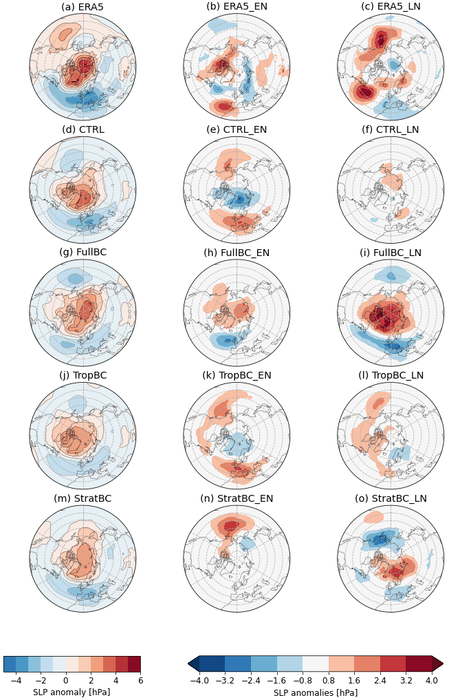
Figure 8 The left column shows composites of absolute SLP anomalies averaged over 30 d after the central dates of SSWs for neutral ENSO conditions for the models and all years for ERA5. The middle and right column show the difference between SLP anomalies during El Niño (middle) and La Niña (right) minus neutral condition anomalies. ERA5 data from 1979–2019, 100 years for each model run (neutral, El Niño, and La Niña).

Figure 9 Heat flux anomaly at 100 hPa, 45–75^∘ N for SSW events composited on day zero of SSWs, defined for wave 1 (red), wave 2 (blue), and all waves (black). In model experiments, the anomalies are calculated with respect to that experiment's climatology. In ERA5, the anomalies for all years as well as for ENSO years are calculated with respect to the ERA5 climatology. ERA5 data from 1979–2019, 100 years for each model run (neutral, El Niño, and La Niña).

3.4 Heat flux and wave 1 $/$ wave 2 ratio response

We now look at the wave forcing that causes SSWs. Figure 9 shows the SSW composite anomalies for the heat flux at 100 hPa, 45–75^∘ N. The black lines show all wave numbers, the red lines are wave 1, and the blue lines are wave 2. Solid lines indicate dates when the composite anomalies are significantly different from zero at the 90 % confidence level. The ratios of wave 1 to wave 2 SSW events are also listed in Table 1, where each event is defined based on the average heat flux for the 10 d preceding an SSW. The CTRL run has a too small wave 1 $/$ wave 2 flux ratio of $\mathrm{62}/\mathrm{38}$ compared to the ERA5 ratio of $\mathrm{77}/\mathrm{23}$; i.e. there are too many wave 2 events in CTRL. ERA5 has 0.15 wave 2 SSWs per year, and CTRL has 0.41 wave 2 SSWs per year. This ratio is improved in the bias correction experiments, with the FullBC ($\mathrm{76}/\mathrm{24}$) being most similar to ERA5, and a smaller improvement in StratBC ($\mathrm{67}/\mathrm{33}$) and TropBC ($\mathrm{68}/\mathrm{32}$). As expected, in ERA5 the wave 2 flux is weaker in El Niño years and stronger in La Niña years; hence, La Niña events have a smaller wave 1 $/$ wave 2 ratio than El Niño events (e.g. Garfinkel and Hartmann, 2008). This is simulated reasonably well in the experiments, but the relationship is weaker. For all climatologies the El Niño years have a larger wave 1 $/$ wave 2 ratio than La Niña years; however, in CTRL the La Niña experiment has a larger wave 1 $/$ wave 2 ratio than the neutral experiment. The total heat flux anomaly before an SSW is smallest in El Niño and largest in La Niña in all climatologies. Since the anomalies are calculated with respect to each experiment's own background flux, which is largest in El Niño and smallest in La Niña experiments, the result explains the larger frequency of SSWs in El Niño and small frequency in La Niña. It happens because during El Niño years, an SSW can be induced by a weaker wave activity pulse, which happen more frequently. However, a larger wave activity pulse that occurs more rarely is required to induce an SSW during La Niña years. Note that in all experiments as well as in ERA5 the larger flux during La Niña years is due to increased wave 2 contribution; however, only in StratBC is the wave 2 increase larger than that of wave 1, which is also seen in ERA 5.

4 Discussion and conclusions

The ECHAM6 atmospheric model was run with bias-correcting tendencies added to the temperature and divergence at each time step. The bias corrections were added at different levels – the stratosphere (StratBC), troposphere (TropBC), or full atmosphere (FullBC) – to create a range of climates with reduced biases. SST forcing experiments were conducted within these climates by applying a positive or negative ENSO pattern in the tropical Pacific. The seasonal mean response is explored in Tyrrell and Karpechko (2021). In this paper we have focused on the relationship between the ENSO forcing and SSWs.

For the years without an ENSO forcing the number of SSWs is overestimated in our control run in comparison with ERA5. This is largely due to the polar vortex being too weak in the CTRL run. When the strength of the vortex is improved in FullBC the SSW statistics also improve. There is an insignificant improvement in the StratBC runs, despite the improvement in the strength of the vortex being similar to FullBC. The polar vortex strength was not corrected in the TropBC run, and there is no significant improvement in the number of SSWs. The lack of stratospheric bias correction in TropBC indicates that the stratospheric biases do not originate in the tropospheric circulation biases but are more likely resulting from orographic and non-orographic gravity wave drag parameterizations (e.g. Eichinger et al., 2020). The seasonal variation in SSWs is too small in the CTRL run compared to ERA5, with too many SSWs in November and March. This is slightly improved in FullBC, but not in StratBC or TropBC. The duration of an SSW is well simulated; i.e. the number of days that UZ <0 m/s after an SSW is not significantly different from ERA5 in any of the model runs, suggesting that it is controlled by basic processes such as radiative relaxation, well represented in the model. Likewise, the downward propagation and surface response is similar between ERA5 and the control run and not affected by the bias corrections. The ratio of wave 1 to wave 2 events is too small in CTRL, and this is improved in FullBC, and to a lesser extent in StratBC and TropBC.

The ERA5 reanalysis data suggest that there is an increase in SSWs in both La Niña and El Niño years, when compared to neutral years (Table 1). This is based on a fairly low number of events; depending on the threshold used to define ENSO there are around 10–15 El Niño or La Niña years, with around 0.6–0.9 SSWs per year. This makes it difficult to statistically confirm the observed ENSO–SSW relationship. Our model results differ from observations and are in line with other modelling studies, which show a more linear relationship between ENSO and SSWs. The increase in wave 1 events in El Niño years and wave 2 events in La Niña years is captured by the bias-corrected runs, but not by the control run. The timescales of variability in the stratosphere were tested with the autocorrelation of Z_cap, and it was found that the weakening (El Niño) and strengthening (La Niña) of the polar vortex due to ENSO phases explain changes to the timescales of the variability. However, similar strength changes to the vortex by the bias corrections did not relate directly into similar changes to the timescales of the variability, suggesting that other factors associated with bias correction procedure affect the timescales.

The impact of ENSO phase on Z_cap response to SSWs was fairly consistent amongst the models, with a weaker lower stratospheric Z_cap SSW relative response (i.e. less warming and less weakened vortex) during El Niño years and stronger Z_cap relative response (more warming and weaker vortex) during La Niña years. This relationship between ENSO phase and the stratospheric SSW response did not consistently lead to a similar relationship between the mean sea level pressure (MSLP) response averaged over 30 d after SSWs amongst the models. All the model runs showed a negative AO response, with FullBC and StratBC having a stronger response in La Niña years and CTRL and TropBC having a weaker response in El Niño years. The composite eddy heat flux showed that a larger anomalous wave forcing is required for an SSW to occur during La Niña years, compared to neutral and El Niño years, and the El Niño anomalous wave forcing required to trigger an SSW was slightly smaller than in neutral years. This relationship is associated with the fact that the anomalous forcing is calculated with respect to each experiment's own climatology, and there is a larger background wave forcing in the El Niño experiments and a smaller wave forcing in the La Niña experiments. Consequently, a relatively small anomalous forcing is required to induce an SSW in the El Niño experiments, and a large anomalous forcing is required in La Niña experiments. The additional wave forcing during La Niña years primarily came from an increase in wave 2 events, and likewise the reduced wave forcing during El Niño years was associated with less wave 2 forcing. This result is similar in the ERA5 data, although with more extreme differences in wave 1 and 2 between the ENSO phases. Indeed, in ERA5 La Niña years the magnitude of wave 2 forcing is greater than that of wave 1, which was only reproduced in the StratBC model runs.

Overall, we show that reductions in both stratospheric and tropospheric biases can improve the SSW statistics of a model in relation to the number of SSWs per year and the ratio of wave 1 and wave 2 events. Whether the improvements lead to a more realistic ENSO–SSW relationship is unclear given the large uncertainty in the observed statistics.