Benefits and challenges of dynamic sea ice for weather forecasts

The drive to develop environmental prediction systems that are seamless across both weather and climate timescales has culminated in the development and use of Earth system models, which include a coupled representation of the atmosphere, land, ocean and sea ice, for medium-range weather forecasts. One region where such a coupled Earth system approach has the potential to significantly influence the skill of weather forecasts is in the polar and sub-polar seas, where fluxes of heat, moisture and momentum are strongly influenced by the position of the sea ice edge. In this study we demonstrate that using a dynamically coupled ocean and sea ice model in the European Centre for Medium-Range Weather Forecasts (ECMWF) Integrated Forecasting System results in improved sea ice edge position forecasts in the Northern Hemisphere in the medium range. Further, this improves forecasts of boundary layer temperature and humidity downstream of the sea ice edge in some regions during periods of rapid change in the sea ice, compared to forecasts in which the sea surface temperature anomalies and sea ice concentration do not evolve throughout the forecasts. However, challenges remain, such as large errors in the position of the ice edge in the ocean analysis used to initialise the ocean component of the coupled system, which has an error of approximately 50 % of the total forecast error at day 9, suggesting there is much skill to be gained by improving the ocean analysis at and around the sea ice edge. The importance of the choice of sea ice analysis for verification is also highlighted, with a call for more guidance on the suitability of satellite sea ice products to verify forecasts on daily to weekly timescales and on meso-scales (< 500 km).

1 Introduction

Dynamic sea ice and ocean have long been recognised as important components in the Earth system models used to generate climate projections (Holland and Bitz, 2003; Manabe and Stouffer, 1980) and more recently in seasonal forecasts (Guemas et al., 2016; Koenigk and Mikolajewicz, 2009; Tietsche et al., 2014). This is to meet the societal demand for information on the future state of the sea ice itself (e.g. Melia et al., 2017; Stephenson et al., 2013) and to capture important climate feedbacks and the remote influence of sea ice on atmospheric circulation (Balmaseda et al., 2010; e.g. Screen, 2017). However, the benefit of sea ice coupling on the timescales relevant for global numerical weather prediction (NWP), i.e. days to weeks, has received less attention.

Until recently it was assumed that sea ice fields change so slowly that it is acceptable to keep them fixed for the period covered by global medium-range weather forecasts, so NWP systems typically only included a simple bulk thermodynamic representation of the sea ice, which enables variations in sea ice surface temperature during the forecast without the additional complexity of varying the sea ice concentration and thickness (e.g. Mironov et al., 2012). However, this is not the case even for 5 d forecasts in the marginal ice zone, where the total ice cover can change by more than 5 % (and 10 %) in the transition seasons in the Northern Hemisphere (and Southern Hemisphere) (Keeley and Mogensen, 2018).

The presence of sea ice dramatically influences turbulent exchange at the surface, particularly in winter, when the overlying atmosphere is much colder than the open ocean. As a result errors in sea ice concentration have the potential to degrade the skill of atmospheric forecasts (Jung et al., 2016). For example, during off-ice atmospheric flow situations in winter months (e.g. during marine cold-air outbreaks, MCAOs), the position of the sea ice edge is a strong control on turbulent exchange (Andreas, 1980). As a result it has been shown in idealised experiments that the geometry and position of the sea ice edge strongly influences boundary layer and cloud development even hundreds of kilometres downstream of the sea ice (Gryschka et al., 2008; Liu et al., 2006; Spensberger and Spengler, 2021) and as a result can influence the track and intensity of hazardous polar lows (Sergeev et al., 2018) on timescales relevant for short- and medium-range NWP.

For these reasons adding sea ice and ocean components to a forecasting system has the potential to increase forecast skill, particularly in locations close to the sea ice edge. Indeed, pioneering efforts with coupled regional NWP systems have shown promising improvements in both sea ice and atmosphere fields compared to atmosphere-only systems (e.g. Pellerin et al., 2004; Smith et al., 2013). Therefore, as part of a drive to develop a forecasting system that is seamless across timescales, the European Centre for Medium-Range Weather Forecasts (ECMWF) took the pioneering step of coupling sea ice cover and sea surface temperatures (SSTs) between the dynamic–thermodynamic ocean–sea ice model NEMO-LIM2 (Nucleus for European Modelling of the Ocean Louvain-la-Neuve sea ice model version 2 ) and ECMWF's Integrated Forecasting System (IFS) for all time ranges, thereby developing the first coupled global medium-range forecasting system including dynamic sea ice (Buizza et al., 2017; Keeley and Mogensen, 2018). In the ensemble context this has the additional benefit that each ensemble member can have its own sea ice and SST fields, consistent with the evolution of the meteorology. However, only deterministic forecasts will be considered in the present study.

Published literature evaluating operational and candidate global coupled NWP systems has been quite broad in scope (Smith et al., 2018; Vellinga et al., 2020) or focused on tropical cyclones (Mogensen et al., 2017). However, little focus has been given to the evaluation of coupled forecast performance in the high latitudes where there is potentially much to gain from coupling the atmosphere with the ocean and sea ice (Jung et al., 2016).

In this study we perform an evaluation of a set of 10 d deterministic forecasts with the coupled IFS, comparing them to an equivalent set of uncoupled forecasts, where observed sea ice concentration and SST anomalies from the initial time of each forecast are persisted throughout the forecast range. This enables us to explore three questions relevant to the ongoing development of coupled NWP systems more generally:

1. On what timescales does dynamic coupling to the ocean–sea ice model produce noticeably improved forecasts of the ice edge?

2. Does skill in forecasting the position of the sea ice edge improve in all conditions or during specific episodes?

3. Is there evidence that the coupling to the dynamic ocean–sea ice has an impact on downstream atmospheric conditions?

2 Methods

2.1 Experiments

To evaluate the impact of ocean and sea ice coupling on sea ice and atmospheric forecasts in the medium range, three sets of 10 d forecast experiments (hereafter referred to as forecasts) were run with the ECMWF IFS for the period DJFM 2017/18. The experiments are initialised each day at 24:00 UTC during the period: one in which dynamic coupling with sea ice concentration and ocean is switched on (coup-SSTSIC), one atmosphere-only where sea ice concentration and SST anomalies are persisted from the initial time (pers-SSTSIC), and another atmosphere-only with updated observed sea ice concentration and SSTs (obs-SSTSIC). These were all run with Cycle 46r1 of the IFS at TCo1279 (∼ 9 km) resolution with 137 vertical levels, which is the current resolution of the operational high-resolution 10 d forecasts at ECMWF.

Table 1 Configuration of experiments.

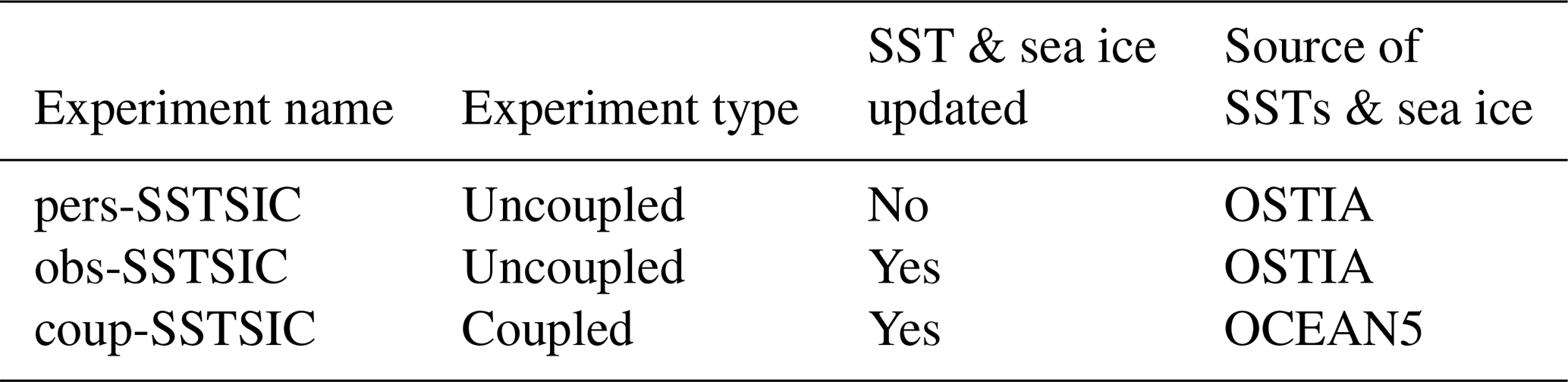
In the uncoupled forecasts (pers-SSTSIC and obs-SSTSIC), sea ice concentration and sea surface temperature (SST) from the Operational Sea Surface Temperature and Sea Ice Analysis (OSTIA; Donlon et al., 2012) are prescribed at the surface. The sea ice fields in OSTIA are derived from the European Organisation for the Exploitation of Meteorological Satellites (EUMETSAT) Ocean and Sea Ice Satellite Application Facility (OSI SAF) sea ice concentration product (Tonboe and Lavelle, 2016) but are interpolated onto the OSTIA grid and adjusted to make the ice concentration consistent with the OSTIA SSTs. In pers-SSTSIC sea ice concentration and the SST anomalies are persisted from the initial time to the end of the forecast, as was done in ECMWF high-resolution operational forecasts until the IFS Cycle 45r1 upgrade in June 2018 (the ECMWF Ensemble forecasts have included dynamic sea ice since the Cycle 43r1 upgrade in November 2016). In this experiment a persisted anomaly approach is used for the SSTs, where the anomaly at the initial time is added to the daily climatology appropriate for each forecast lead time. In the other uncoupled experiment, obs-SSTSIC, the SST and sea ice fields are updated daily throughout the forecast, again using OSTIA. This experiment allows one to assess the maximum potential benefit of correctly representing SSTs and sea ice for atmospheric forecast skill (assuming the evolution of the overlying atmosphere is consistent with the sea ice changes).

The OSTIA fields used in the ECMWF operational analysis (during the period used in this study) are updated daily at 12:00 UTC and fixed until the next day at the same time. The OSTIA analysis fields are based on observations collected during a 36 h window centred on 12:00 UTC the previous day (Donlon et al., 2012). As a result the sea ice concentration and SST fields used in the pers-SSTSIC and obs-SSTSIC runs are approximately 36 h old at the initial time.

For the coupled forecasts (coup-SSTSIC), the IFS atmosphere is coupled to NEMO (Madec, 2008) model version 3.4.1 and LIM2, using the ORCA025 horizontal grid (with a resolution of approximately ∼ 10 km in the Arctic) with 75 levels in the vertical. The IFS makes use of a single executable framework, using a sequential coupling procedure described in Mogensen et al. (2012). Operationally the only sea ice model variable that is coupled to the atmosphere is the sea ice cover. For the SSTs the atmosphere and ocean are fully coupled in the tropics at all lead times but only partially coupled in the extra-tropics to avoid SST biases that would degrade forecast skill. In these regions of partial coupling, during the first 4 d of the forecast, rather than the atmosphere seeing the actual SST field from the ocean model, SSTs from OSTIA are provided at the initial time. These are then updated by adding the SST tendencies from the ocean model onto the initial field.

In the coupled forecasts, the ocean and sea ice fields are initialised from the ECMWF OCEAN5 analysis (Zuo et al., 2019). OCEAN5 uses the same NEMO-LIM2 model used in the coupled forecasts, forced by atmospheric forecast fields at the surface, and assimilates observations using the NEMOVAR 3D-Var assimilation system. OSTIA sea ice concentration and SSTs are assimilated in its production in addition to other ocean data sources. The atmosphere of all three experiments is initialised from the ECMWF operational analysis.

2.2 Verification data and metrics

2.2.1 Sea ice edge evaluation

We compare the coupled and uncoupled sea ice forecasts using the integrated ice edge error (IIEE) metric (Goessling et al., 2016), which measures the skill of forecasts of the ice edge. It is defined as the total area where the forecast and the observations disagree on the ice concentration being above or below a given value, that is, the sum of all areas where the local sea ice extent is overestimated (O) or underestimated (U): IIEE = O + U. Since this metric captures spatial information on the position of the sea ice edge, it is a natural choice for evaluating the impact of including sea ice dynamics over a given region.

An ice concentration of 20 % was used as the ice-free–ice-covered threshold in the IIEE calculation, instead of 15 % (as used in Goessling et al., 2016), to facilitate a fair comparison between the coup-SSTSIC and pers-SSTSIC forecasts. This is because in the pers-SSTSIC experiment ice concentrations of less than 20 % were set to zero, as was done in operations at ECMWF prior to the implementation coupled system.

2.2.2 Verifying analysis

In the IIEE and other metrics, the daily mean sea ice concentration from the forecasts (calculated from 6-hourly fields at 06:00, 12:00, 18:00 and 00:00 UTC) is compared with the operational OSI SAF analysis (OSI-401-b) for the appropriate day (Tonboe and Lavelle, 2016) to evaluate the sea ice forecast skill. The choice of analysis to use for verification is a complex issue and has received significant attention for atmospheric fields in NWP, where one needs to objectively determine whether one version of a forecasting system is better than another to advance forecast skill (Geer, 2016). There is, however, little guidance for sea ice evaluation on NWP timescales, so some subjective evaluation is performed against the Moderate Resolution Imaging Spectroradiometer (MODIS) in Sect. 3.1.

Atmospheric forecast fields are evaluated against the ERA5 reanalysis (Hersbach et al., 2020). Although ERA5 is produced at a lower resolution and with an older version of the IFS than the experiments in this study, ERA5 does not have the 36 h lag in the OSTIA SST and sea ice boundary conditions present in the operational analysis and should therefore provide a better estimate of the atmospheric state at the sea ice edge. Therefore the evolution of the sea ice and atmospheric boundary layer should be more consistent than in the operational analysis.

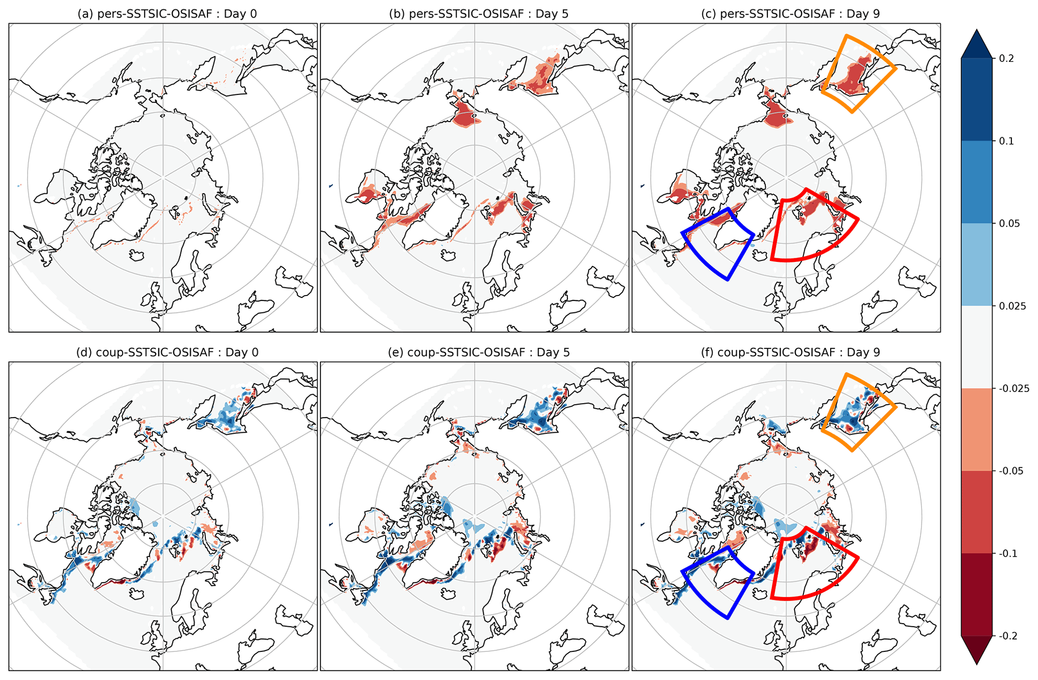
Figure 1 Daily mean sea ice concentration bias, relative to OSI SAF for the persisted forecasts, pers-SSTSIC (a–c), and the coupled forecasts, coup-SSTSIC (d–f), at a lead time of 0 d (a, d), 5 d (c, e) and 9 d (e, f). The Nordic Seas (red), Labrador and North-East Atlantic region (blue), and Sea of Okhotsk (orange) are highlighted by the coloured boxes in the right-hand column.

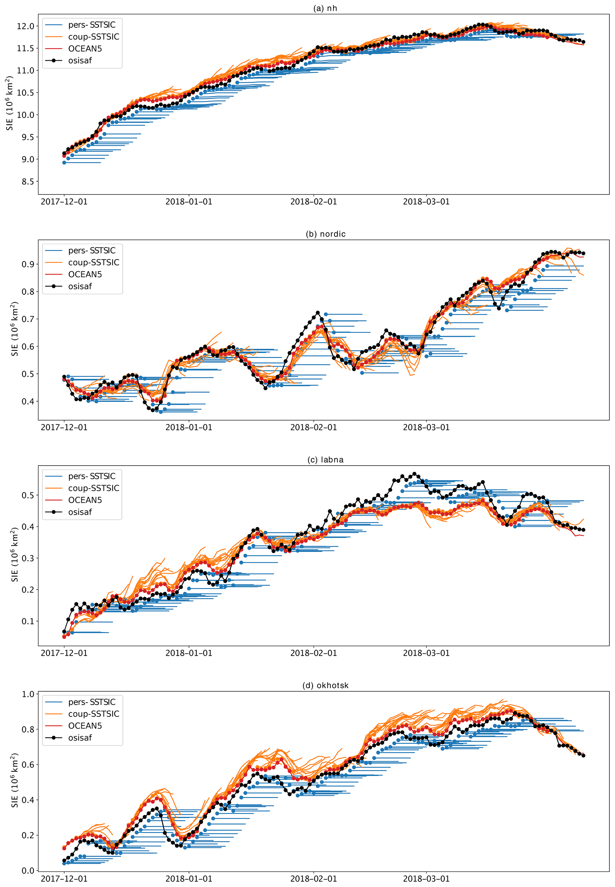
Figure 2 Time series of sea ice extent in the Northern Hemisphere (a), Nordic Seas region (b), Labrador and North-East Atlantic (c), and the Sea of Okhotsk (d). The regions are shown in Fig. 1. Daily mean sea ice extent for each 10 d forecast and each analysis product is plotted with day 0 indicated by a dot marker. The date is given in the format year-month-day.

3 Results

3.1 Sea ice forecast skill

Since the forecast experiments were performed for winter (DJFM), which is a period of ice expansion in the Northern Hemisphere, persisting sea ice (in the pers-SSTSIC runs) results in negative ice concentration (Fig. 1a) and extent (Fig. 2) biases which grow with lead time. The pattern of the bias is more complicated in the coup-SSTSIC (Fig. 1d–f). The bias is corrected, by construction, in the obs-SSTSIC runs (not shown) and improved relative to pers-SSTSIC in some regions in the coup-SSTSIC runs since the ice extent is free to increase (or decrease) in the coupled model.

In some regions the coup-SSTSIC forecasts exhibit a positive bias. This is particularly the case in the region north of Svalbard, along the Labrador Sea coast of North America and in the Sea of Okhotsk (Fig. 1), as can also be seen in the time series of Northern Hemisphere sea ice extent (Fig. 2a). The spatial pattern of the bias in the coupled forecasts is consistent across lead times, but the magnitude increases. This suggests that the pattern of the bias, with respect to OSI SAF, is present in the OCEAN5 analysis, i.e. already at the initial time of the forecast, and is inherited from biases in the background forecasts from the ice–ocean model, which advances the ice edge too rapidly, consistent with the findings of Tietsche et al. (2015) and further discussed in Sect. 3.2.

For objective scoring of the forecasts, we calculate the IIEE with respect to OSI SAF, which provides an integrated measure of forecast performance for the position of the sea ice edge in a given region. It provides a detailed picture of how accurate the forecasts are in predicting which grid boxes are covered with sea ice by taking misplacement of the ice as well as the total area of ice into account (Goessling et al., 2016). It was calculated for the Northern Hemisphere as a whole and also for the Nordic Seas (65–83^∘ N, 20^∘ W–60^∘ E), western Atlantic/Labrador Sea region (55–70^∘ N, 62–30^∘ W) and the Sea of Okhotsk (45–62^∘ N, 135–157^∘ E). These regions are shown in the coloured boxes in Fig. 1c and f.

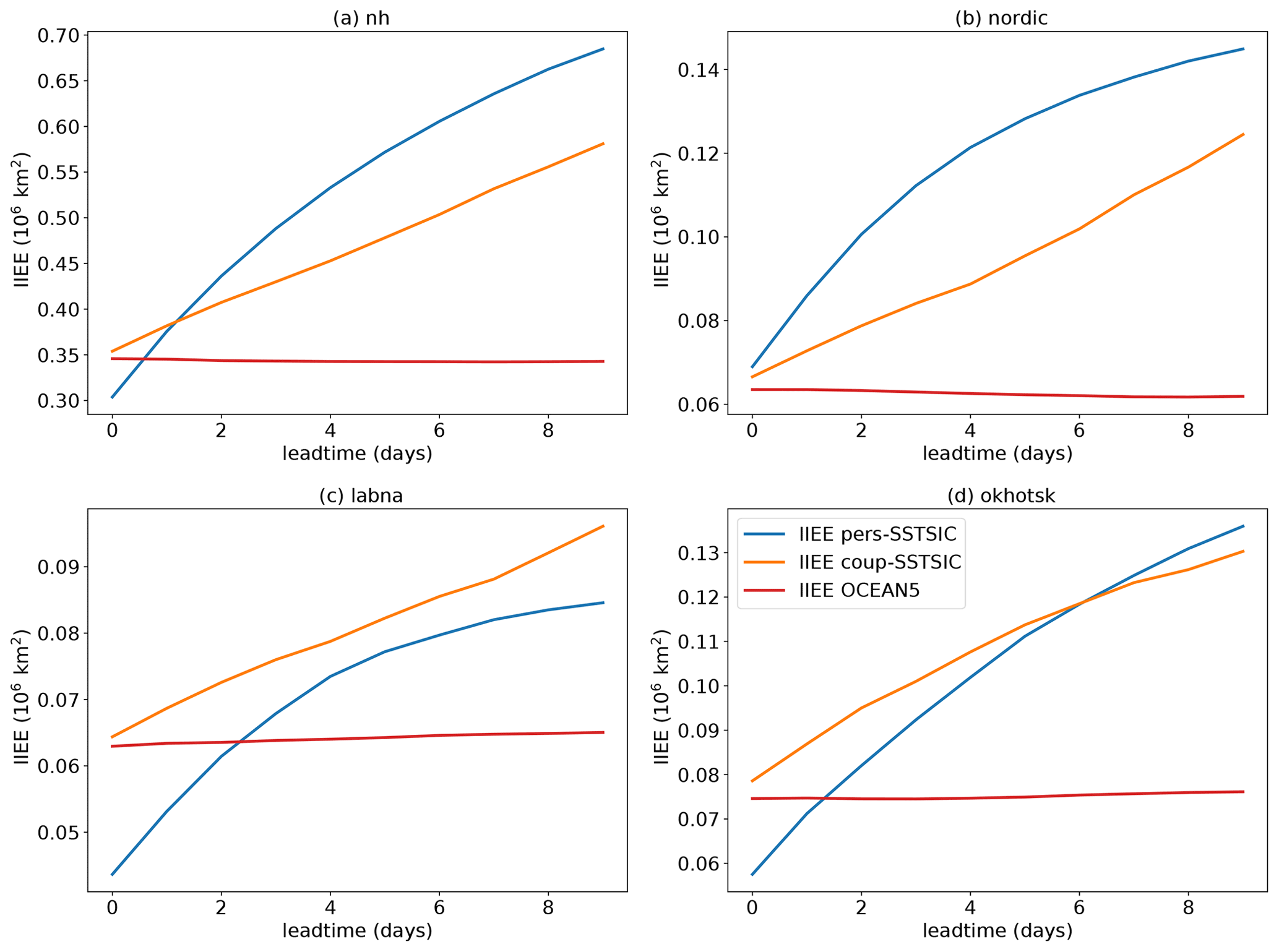
Figure 3 Average integrated ice edge error (IIEE) over all forecasts plotted against lead time, for the whole Northern Hemisphere (a), the Nordic Seas (b), and the Labrador–North-East Atlantic (c) and the Sea of Okhotsk (d) regions. These regions are shown in Fig. 1c and f.

IIEE increases with lead time for both pers-SSTSIC and coup-SSTSIC, with pers-SSTSIC generally increasing more rapidly. The lead time at which coup-SSTSIC becomes more skilful than pers-SSTSIC, based on the IIEE, varies from region to region. In the Northern Hemisphere and Nordic Seas region, coup-SSTSIC shows an improvement early in the forecast. However, the coup-SSTSIC forecasts have a larger IIEE in the Labrador and North-East Atlantic region at all lead times and in the Sea of Okhotsk until day 6. If, and at what lead time, the coupled forecast becomes more skilful depends on both the size of the initial error in coup-SSTSIC and the rates of error growth of both the coupled model and a persistence forecast. All these factors are regionally dependent: for example, in the Sea of Okhotsk there is a large initial bias in ice extent which grows with lead time, leading to worse performance than persistence during the first 6 d. In contrast the coup-SSTSIC initial error in the Nordic Seas is smaller than pers-SSTSIC and biases are more modest, and so performance is better than persistence from day 0. The skill of a persistence forecast will also vary from region to region based on the local ice dynamics.

It is interesting to note the large initial (day 0) IIEE in both pers-SSTSIC and coup-SSTSIC experiments. Errors in the pers-SSTSIC forecast at day 0 are partly due to the lag in the time at which sea ice fields are available to the operational analysis (see Sect. 2.1 for explanation) and partly due to small differences between the OSI SAF fields, used for evaluation, and OSTIA fields, used as boundary conditions for the model, due to interpolation and adjustment for consistency with the SSTs used in the OSTIA product.

Initial errors in coup-SSTSIC are inherited from the OCEAN5 analysis (also noted by Zampieri et al., 2018) as indicated by the similarity between the coup-SSTSIC IIEE at day 0 and the IIEE of OCEAN5 with respect to OSI SAF (i.e. comparing the orange and red curves in Fig. 3). It is worth noting that the coup-SSTSIC day-0 error for the Northern Hemisphere, with respect to OSI SAF, is more than 50 % of the IIEE of the coupled forecast at day 9. It is also striking that the error in the analysis, expressed as the IIEE of the OCEAN5 fields, is larger than the difference in IIEE between the coup-SSTSIC and pers-SSTSIC forecasts (Fig. 3), which suggests that using OCEAN5 instead of OSI SAF for verification would dramatically change the outcome of the evaluation. The next section will focus on evaluation of OCEAN5 sea ice concentration fields.

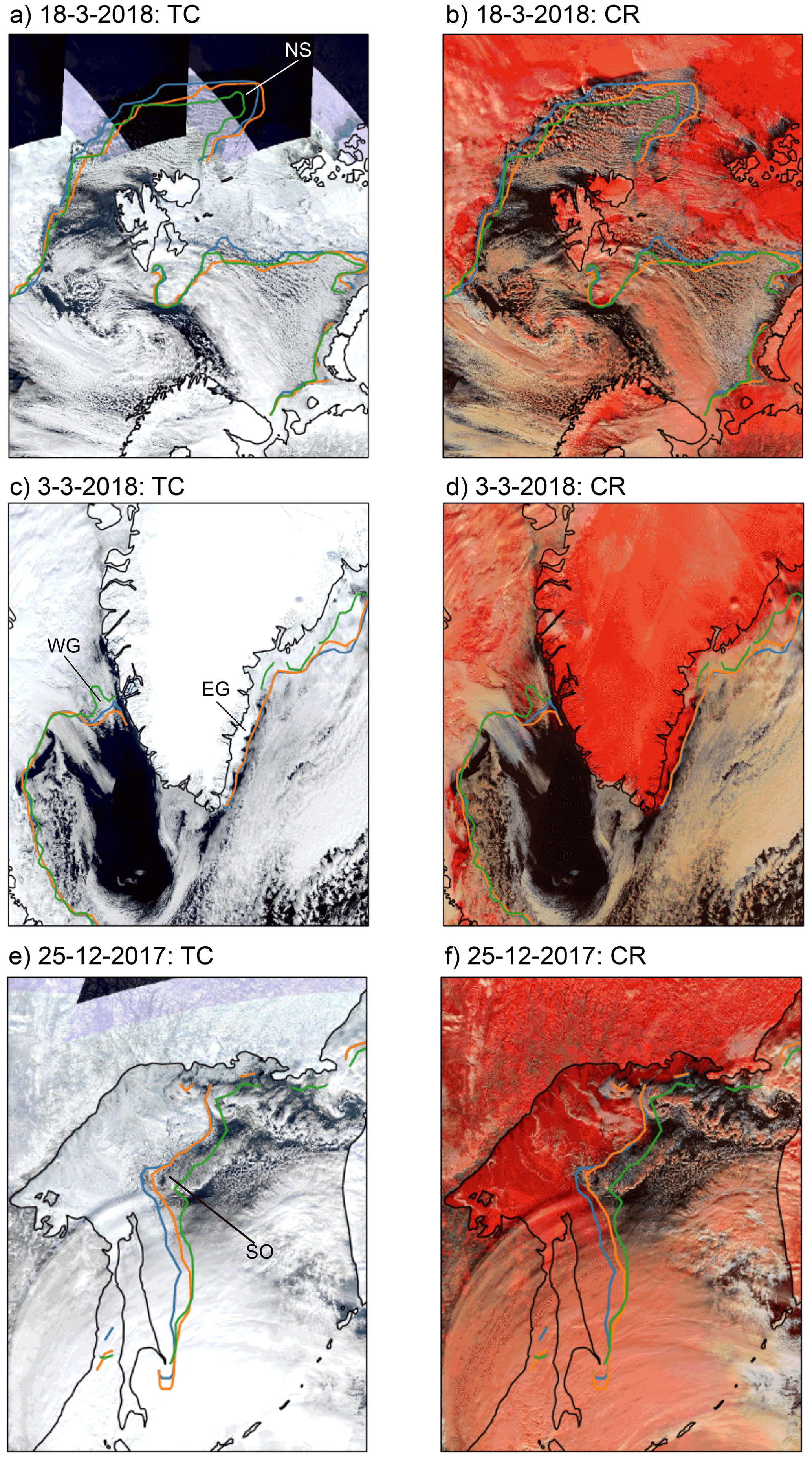
Figure 4 MODIS True Color (a, c, e) and Corrected Reflectance (b, d, f) images for the Nordic Seas on 18 March 2018 (a, b), Labrador and North-East Atlantic region on 3 March 2018 (c, d), and Sea of Okhotsk on 22 December 2017 (e, f). The 0.2 ice fraction contours from OSI SAF (blue), OSI SAF 1 d (orange) and ECMWF OCEAN5 (green) are overlaid. These regions are shown by the coloured boxes in Fig. 1c and f. Areas of large discrepancy between the OCEAN5 analysis and MODIS images are annotated.

3.2 Subjective evaluation of the initial analysis (OCEAN5)

Subjective evaluation of the sea ice edge position in the OSI SAF and ECMWF OCEAN5 analyses against True Color and Corrected Reflectance images from the Moderate Resolution Imaging Spectroradiometer (MODIS) for selected forecast dates confirms the day-0 differences seen in Figs. 1–3. In the MODIS Corrective Reflectance product (shown in Fig. 4b, d and f) snow and ice appear bright red. Thick ice and snow appear vivid red (or red-orange), while ice crystals in high-level clouds appear reddish-orange or peach. Open ocean appears dark, but small liquid water drops in clouds appear white. This strong contrast between the red (sea ice) and the dark (open ocean) shades in the images can be used to infer the position of the sea ice edge.

Overall, the OSI SAF sea ice edge is more consistent with the MODIS images than the OCEAN5 ones, which further justifies the use of OSI SAF as the reference data for the sea ice verification in this study. The largest difference between OSI SAF and OCEAN5 in the Nordic Seas is in the region north and west of Svalbard (Fig. 1d). A large area of open water is present in this region, and OCEAN5 overestimates the extent of the sea ice (see the region annotated “NS” in Fig. 4a), with the OSI SAF ice edge being a closer match to the MODIS image (i.e. comparing the line contours to the edge of the red ice-covered area in Fig. 4b). In the western Atlantic the differences between OSI SAF and OCEAN5 are largest in the regions adjacent to the east and west coast of Greenland, where OSI SAF is more extensive, stretching further south along both coastlines than in OCEAN5 (Fig. 4c and d). On 3 March 2018 there is a clear discrepancy along the eastern coast of Greenland for example (in the region annotated “EG” in Fig. 4c), where ice is completely missing in the OCEAN5 but present in MODIS and OSI SAF. There is a similar situation in the northern part of the Sea of Okhotsk (in the region indicated with the initials SO in Fig. 4e), where OCEAN5 is more extensive than the OSI SAF fields. The truth is harder to see for the bias west of Greenland, indicated by WG in Fig. 4c, due to the high level of cloud cover in the image shown and in others that were inspected on different dates that are not shown.

In Fig. 4 the OSI SAF fields from the previous day are plotted in orange to provide an indication of how large the difference one would expect from the OCEAN5 field simply due to a lag in the sea ice concentration (SIC) field used in the assimilation. The similarity between the OSI SAF fields from one day to the next and the difference between these and the OCEAN5 fields suggest that errors in the OCEAN5 are systematically biased in these regions, rather than due to a simple lag in the availability of sea ice concentration data for use in the production of the ocean analysis mentioned in Sect. 2.2.1. The fact that biases in these regions show pronounced growth with lead time (see Figs. 1 and 2) further supports the idea that these biases are inherited from the ice–ocean model via the background fields used in the assimilation process. This can be seen most clearly in the time series of sea ice extent for the Sea of Okhotsk where there is a systematic positive bias in the OCEAN5 analysis (red dots) compared to OSI SAF (black dots), which grows with lead time during the forecasts (orange lines; see Fig. 2d).

Another factor is the assimilation methodology: in the NEMOVAR 3D-Var used in OCEAN5, the minimisation of the cost function for sea ice is separate from temperature and salinity (Zuo et al., 2019), so increments in sea ice concentration will not necessarily be consistent with other fields. This may be a particular issue around the sea ice edge, which is quite poorly sampled in terms of in situ observations of temperature and salinity. Another potential avenue for development is the use of observational error estimates for sea ice concentration. These are provided by OSI SAF and OSTIA but are not currently utilised in the data assimilation process.

Figure 5 Time series of day-3 integrated ice edge error (IIEE) of all forecasts for the whole Northern Hemisphere (a), the Nordic Seas (b), and the Labrador–North-East Atlantic (c) and the Sea of Okhotsk (d) regions. These regions are shown in Fig. 1c and f. The date is given in the format year-month-day.

3.3 Improved sea ice forecasts during periods of ice advance and retreat

In this section we investigate whether the difference in skill between pers-SSTSIC and coup-SSTSIC is consistent across the period of study or is larger during specific episodes. Time series of the IIEE at day 3 (Fig. 5) and day 9 (Fig. S1 in the Supplement) show that in general the pers-SSTSIC forecasts are more variable in all regions at both lead times, except for the Sea of Okhotsk at day 3. However, the magnitude of the IIEE is highly variable from day to day, with the values of the IIEE varying by as much as an order of magnitude between the most and least skilful forecasts, depending on the region. This high variability in the error in pers-SSTSIC shows that persistence is at times a very good forecast but that at times it is very poor. Decomposing the IIEE of the pers-SSTSIC forecast into the absolute extent error (AEE) and misplacement error (ME) (following Goessling et al., 2016) allows us to investigate this further.

On average the AEE and ME contribute roughly 50 % each (Fig. S2 in the Supplement) during the period investigated (DJFM), although this ratio may depend on the season. However, further inspection of the time series reveals that situations where persistence is a poor forecast tend to be where the AEE, rather than ME, is large for the persistence forecast (Fig. S2), with the AEE explaining ca. two-thirds of the variance in the IIEE in each region. This shows that the reason that persistence forecasts are particularly poor in these episodes is because rapid expansion and contraction of the area covered with ice is missed.

Figure 6 Scatter plot of difference in IIEE between coup-SSTSIC and pers-SSTSIC forecasts at day 3 (a, c, e) and day 9 (b, d, f) and the change in observed ice extent between the initial time and the verification time for the Nordic Seas (a, b) and the Labrador–North-East Atlantic (c, d) and the Sea of Okhotsk (e, f) regions. These regions are shown in Fig. 1c and f. Colours correspond to the lowest (green), middle (blue) and highest (red) terciles of ice extent change.

These periods of rapid sea ice change are exactly the situations where one would expect the dynamic coupling to add the most value. This can be seen most intuitively from Fig. 2, which shows that pers-SSTSIC is a particularly poor forecast during periods of rapid extent change. During periods where the observed extent increases (decreases), the persistence forecast is biased low (high). As the sea ice in the coup-SSTSIC forecasts is dynamic, the model is able to follow these variations seen in the observations. As a result, the reduction in IIEE (IIEE_coup-SSTSIC − IIEE_pers-SSTSIC) is largest during periods of rapid ice extent change. There is a significant correlation between IIEE_coup-SSTSIC − IIEE_pers-SSTSIC and the magnitude of the observed change in ice extent between the initial and verification times in the Nordic, Labrador and Okhotsk seas at day 3 (r is −0.48, −0.47 and −0.35, respectively, all highly significant) and day 9 (r is −0.54, −0.62 and −0.61, respectively, all highly significant) (see Fig. 6). Indeed, even for lead times where IIEE_coup-SSTSIC is larger than IIEE_pers-SSTSIC on average (e.g. day 3 in the Sea of Okhotsk – Fig. 4d), events with exceptionally large changes in extent are better forecasted by coup-SSTSIC (see e.g. Fig. 6e). This confirms quantitatively what one can see intuitively in Fig. 2.

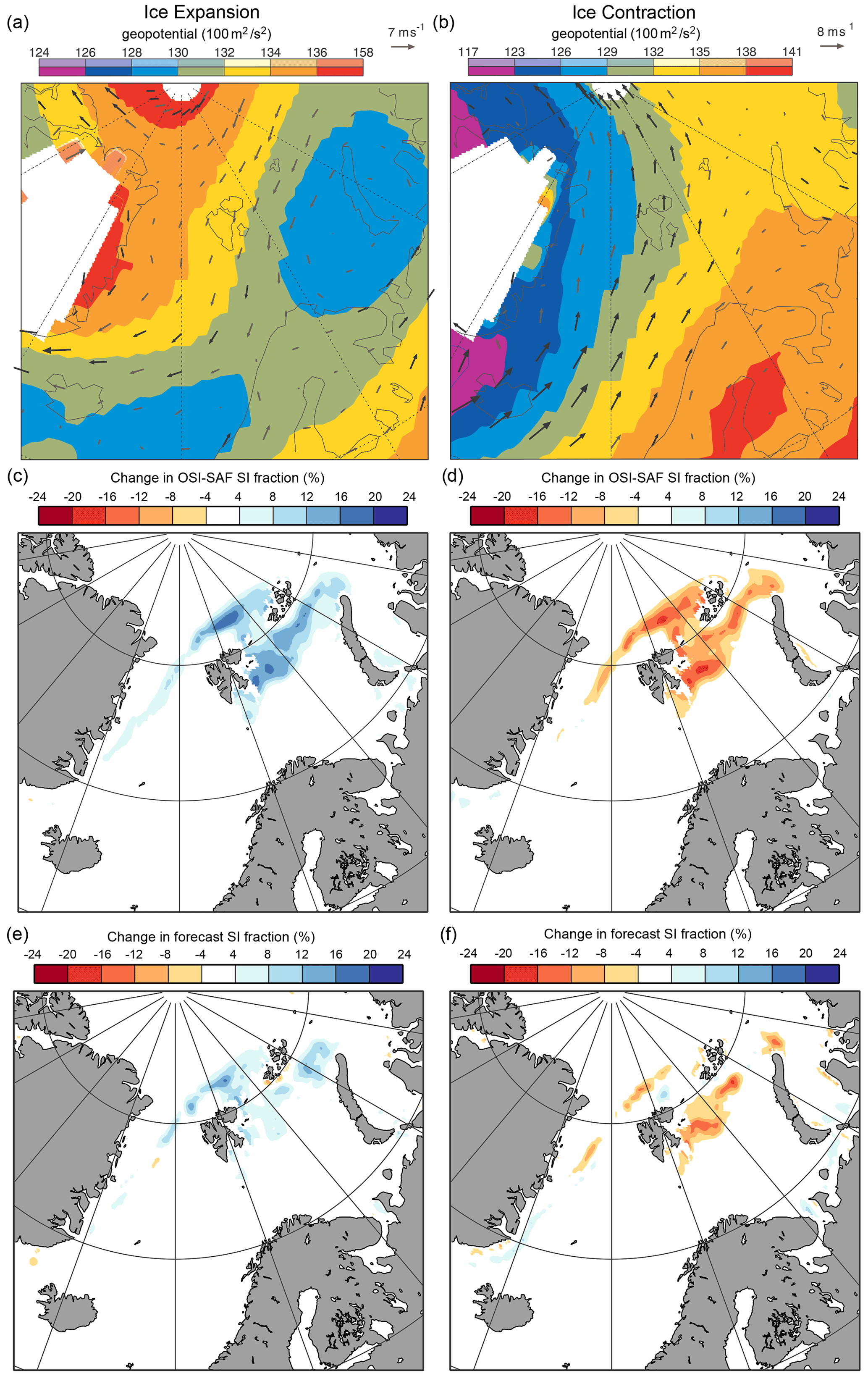
Figure 7 Composite 850 hPa geopotential and vector winds for ice advance (a) and retreat (b) cases selected based on the upper and lower tercile of the 3 d change in sea ice extent (SIE) in the Nordic Seas (highlighted in Fig. S2). Panels (c) and (d) are as (a) and (b) but for the 3 d change in observed SIC. Panels (e) and (f) are as (c) and (d) but for the coupled forecast.

Periods of rapid ice extent change involve either an advancing or a retreating sea ice edge. Splitting the forecast dates into terciles, based on the observed change in sea ice extent over the first 3 d of the forecast, and compositing the initial conditions demonstrate that mean north-easterly (south-westerly) flow is associated with advances (retreat) in sea ice cover in the Nordic Seas region (see Fig. 7a and b). During north-easterly (south-westerly) flow situations southward (northward) advection of the sea ice due to anomalous wind stress and antecedent conditions for thermodynamic growth (melt) leads to a positive 3 d change in sea ice concentration (Fig. 7c and d). Comparison of these composites with the forecast 3 d change in concentration shows that the forecast does not increase as rapidly as seen in observations (Fig. 7e and f). These behaviours can also be seen in the time series of sea ice extent in Fig. 2b, where it can be seen that sea ice extent in coup-SSTSIC does not increase as rapidly as OSI SAF during a period of rapid ice growth in late January 2018 or the subsequent period of rapid decline in early February 2018 in the Nordic Seas. A similar picture can be seen in the other sectors (not shown). Note that the larger IIEE improvement in ice advance cases compared to ice retreat cases likely reflects a positive bias in the rate of ice growth, which tends to favour performance during ice advance.

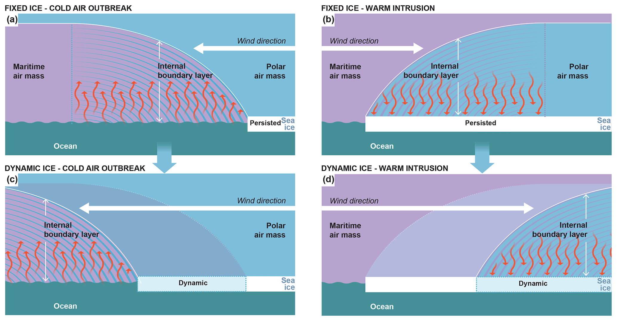
Figure 8 Schematic showing the of impact of dynamic sea ice on turbulent exchange and atmospheric boundary layer development during cold-air outbreaks (a, c) and moist intrusions (b, d).

3.4 Potential benefits of ice–ocean coupling for atmospheric forecasts

As air is advected across a boundary between distinct surface types, such as between sea ice and open water (as in the situation shown in Fig. 6), its properties are modified as it adjusts to the new set of boundary conditions (Oke, 1987). This modification begins at the surface and is propagated upwards through turbulent diffusion. The layer of air whose properties have been affected by the new surface is called an internal boundary layer, and its depth grows with distance downstream of the boundary between the media, known as the leading edge, which in our case is the edge of the sea ice. Here we will focus on variations in the sea ice edge due to their large spatial scale (and therefore importance to global NWP); however air-mass advection between ice-covered and open-water regions in the form of leads and polynyas within the ice is also known to strongly affect air-mass properties (Moore et al., 2002; Pinto and Curry, 1995).

Two such idealised situations are represented in schematics in Fig. 8a and b. Figure 8a shows a situation with off-ice flow, typically seen during marine cold-air outbreaks, where a cold polar air mass is advected across the sea ice edge and over the open ocean. Since this air is much colder and drier than conditions at the surface of the open ocean, upward sensible and latent heat fluxes are induced which act to warm and moisten the internal boundary layer (Renfrew and King, 2000; Spensberger and Spengler, 2021). Conversely, Fig. 8b shows an idealised on-ice-flow situation where a marine air mass is advected over the sea ice. Since this air mass is much warmer and more humid than conditions at the surface, anomalous downward sensible and latent heat fluxes are induced which act to cool and dry the internal boundary layer (e.g. Pithan et al., 2016, 2018).

This link between the position of the sea ice edge and the development of the downstream boundary layer is a potential source of error in forecasts where the sea ice is persisted from the initial analysis, as in pers-SSTSIC. Because the sea ice concentration is itself modified by anomalous surface wind stress and surface energy fluxes, during the situations described above, the position of the leading edge changes over time, influencing downstream boundary layer development. In particular, during persistent off-ice flows, the sea ice edge advances to cover more of the open ocean (see Fig. 8c). As a result, the polar air meets the open ocean further to the south, and the maximum in the turbulent fluxes is shifted further to the south. During persistent on-ice flows the opposite occurs, with the sea ice edge retreating to expose more open water (Fig. 8d). As a result the sea ice dynamics modify the point at which the air-mass transformation begins to occur. The impact that the ice dynamics can have on the internal boundary layer development and on the turbulent fluxes can be seen by comparing Fig. 8a and b, which show an idealised situation where the sea ice has been fixed, with Fig. 8c and d, respectively, which show the same situation but where the sea ice has been allowed to evolve dynamically. The difference in the position of the internal boundary layer is shown in faded hues.

The features described above can be clearly seen in the composites of mean temperature and specific humidity forecast errors during periods of ice advance (Figs. 8–10) and retreat (Figs. S3–S5 in the Supplement) in each of the three regions (shown in Fig. 1c) from the pers-SSTSIC forecast set during DJFM. The dates used in these composites are those for which the 3 d change in sea ice extent is in the top or bottom tercile, as used in Fig. 6.

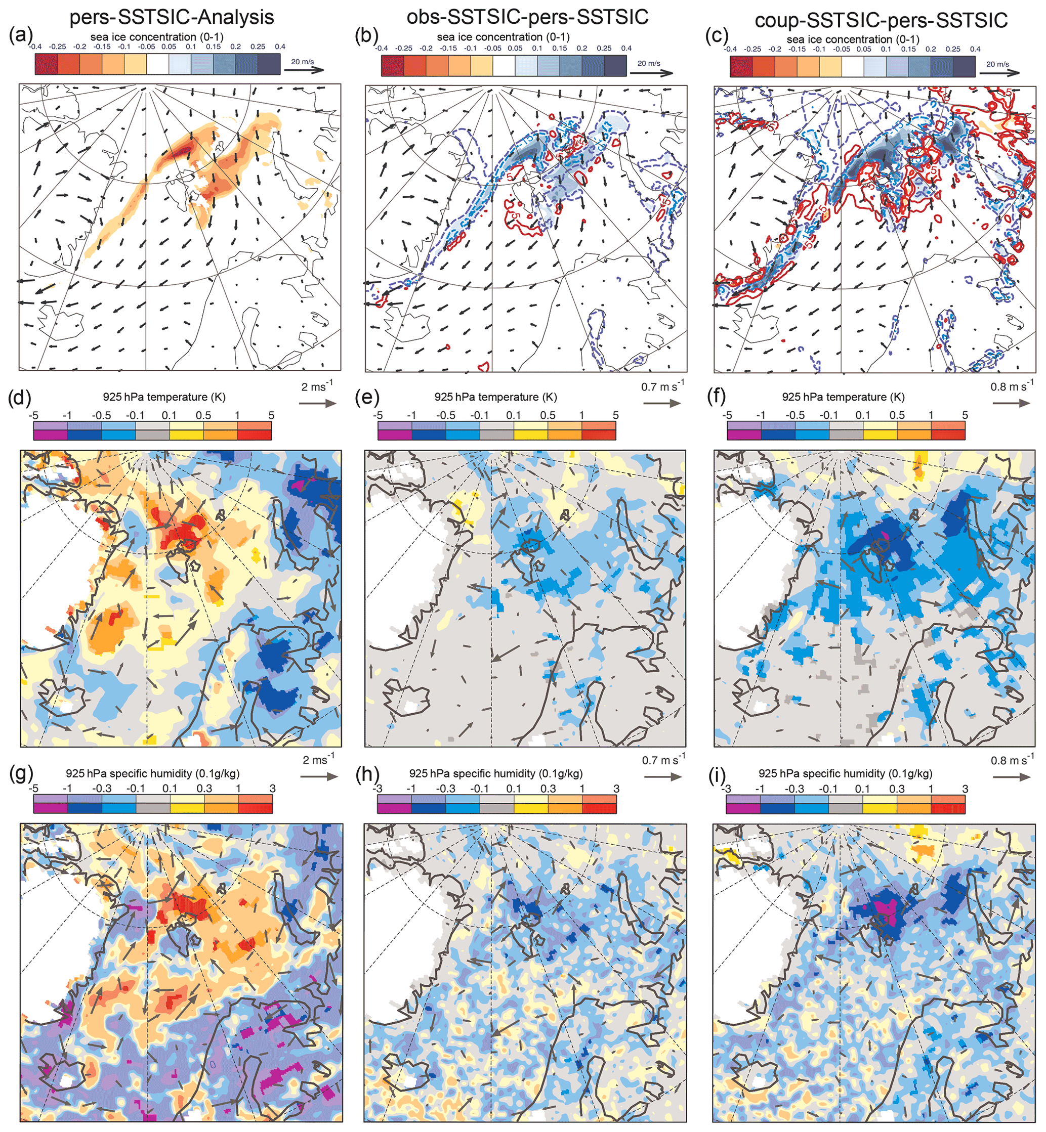
Figure 9 Composite of forecast error during periods of ice advance in the Nordic Seas: day-3 sea ice concentration bias along with composite-mean winds at 925 hPa (a), T + 72 925 hPa temperature and horizontal wind bias (d), and specific humidity and horizontal wind bias (g) for the pers-SSTSIC forecasts and the change in the bias for obs-SSTSIC (b, e and h) and coup-SSTSIC (c, f and i) with respect to the pers-SSTSIC forecasts. The change in the turbulent heat flux (sensible + latent accumulated between T + 48 and T + 72) is shown in the blue and red contours in (b) and (c) (anomalies are positive downwards). In panels (d–i), saturated colours indicate mean differences that are statistically significant at the 5 % level.

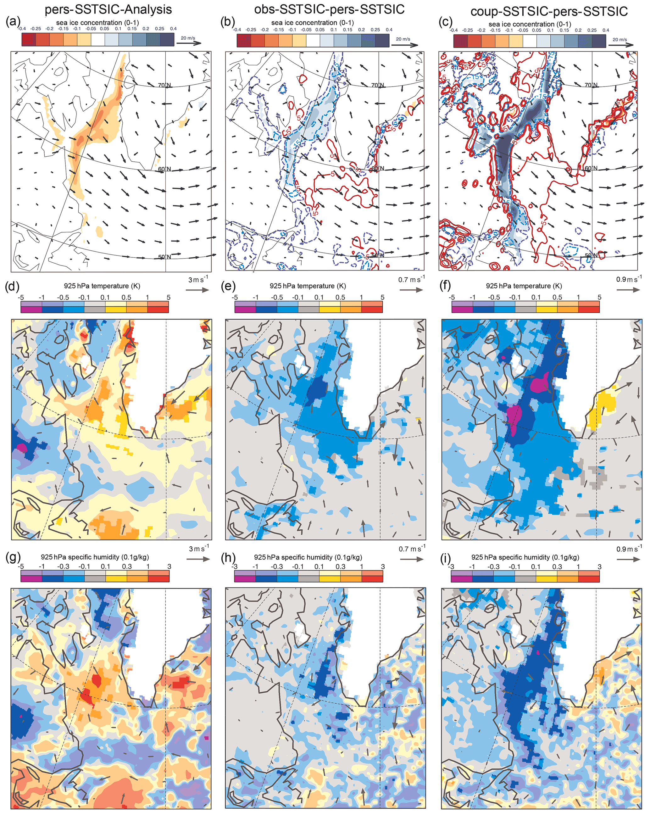
Figure 10 Composite of forecast error during periods of ice advance in the Labrador Sea and Baffin Bay: day-3 sea ice concentration bias along with composite-mean winds at 925 hPa (a), T + 72 925 hPa temperature and horizontal wind bias (d), and specific humidity and horizontal wind bias (g) for the pers-SSTSIC forecasts and the change in the bias for obs-SSTSIC (b, e and h) and coup-SSTSIC (c, f and i). The change in the turbulent heat flux (sensible + latent accumulated between T + 48 and T + 72) is shown in the blue and red contours in (b) and (c) (anomalies are positive downwards). In panels (d–i), saturated colours indicate mean differences that are statistically significant at the 5 % level.

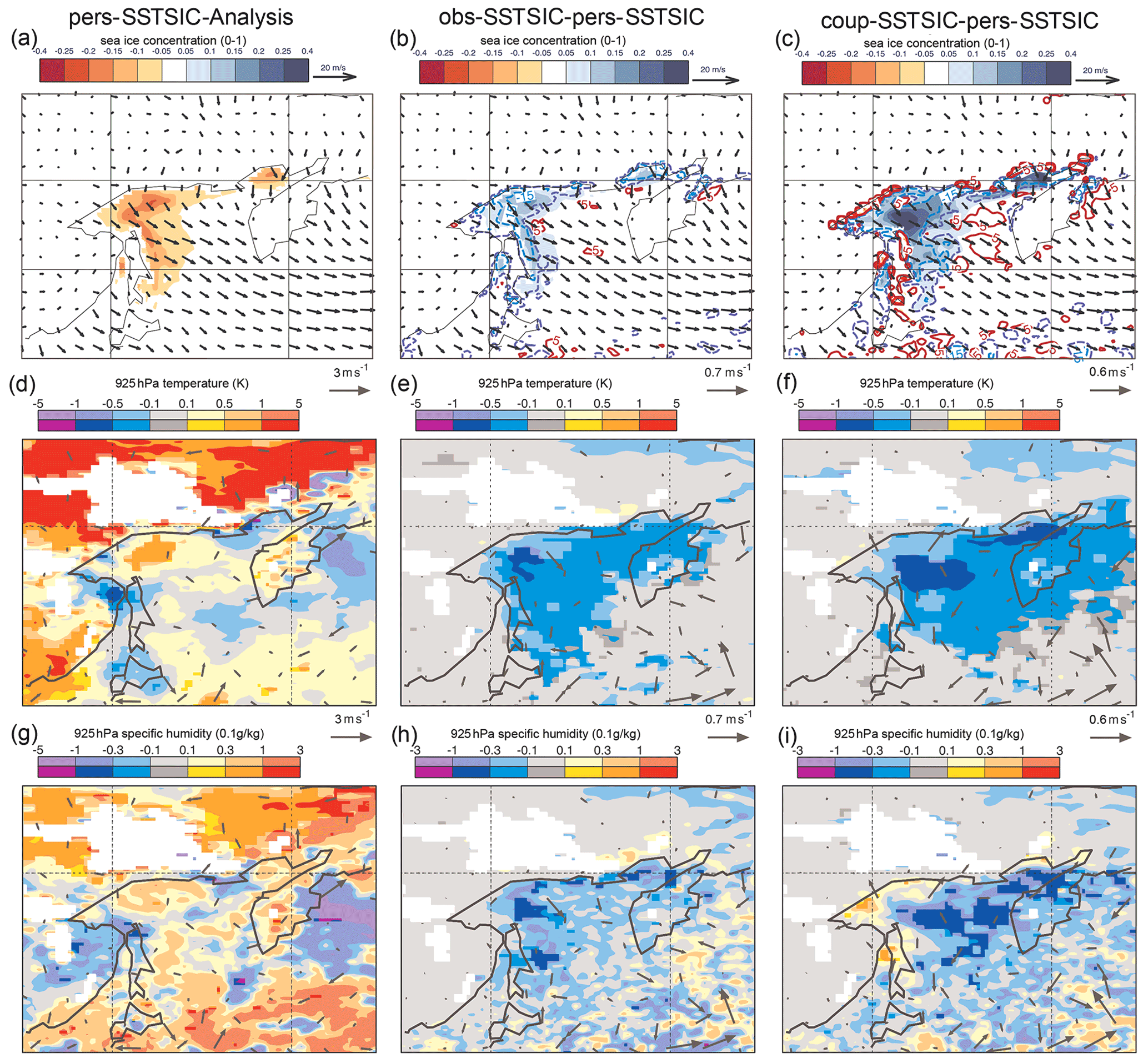
Figure 11 Composite of forecast error during periods of ice advance in the Sea of Okhotsk: day-3 sea ice concentration bias along with composite-mean winds at 925 hPa (a), T + 72 925 hPa temperature and horizontal wind bias (d), and specific humidity and horizontal wind bias (g) for the pers-SSTSIC forecasts and the change in the bias for obs-SSTSIC (b, e and h) and coup-SSTSIC (c, f and i). The change in the turbulent heat flux (sensible + latent accumulated between T + 48 and T + 72) is shown in the blue and red contours in (b) and (c) (anomalies are positive downwards). In panels (d–i), saturated colours indicate mean differences that are statistically significant at the 5 % level.

The negative bias in ice concentration in pers-SSTSIC, during periods of ice advance, goes hand in hand with positive temperature and specific humidity bias around and to the south of the sea ice edge (Figs. 9a, d, g; 10a, d, g; and 11a, d, g). The coup-SSTSIC and obs-SSTSIC forecasts have higher sea ice concentrations than the pers-SSTSIC forecasts (Figs. 9b, c; 10b, c; and 11b, c), and, as a result, the turbulent heat flux (THF) is reduced in those regions. Because the area south of the sea ice edge is a local maximum of THF field and the ice edge is further south in these simulations compared to the uncoupled runs, the THF is increased somewhat to the south, resulting in a dipole in the heat flux field (i.e. dashed red contours to the south of the blue). This effect was also observed in studies with more dramatic changes in sea ice (Day et al., 2012; Deser et al., 2010).

During periods of ice advance obs-SSTSIC and coup-SSTSIC are cooler and generally drier than pers-SSTSIC in the region downstream of the sea ice edge (Figs. 8e, f, h, i; 9e, f, h, i; and 10e, f, h, i); this difference is larger where the difference in sea ice concentration is greatest but extends some ∼ 800 km downstream to the south of the region where the sea ice has changed. To put this into context, the maximum 925 hPa specific humidity difference relative to pers-SSTSIC is perhaps 0.2 g kg⁻¹ northeast of Svalbard. At day 3 in that region the climatological humidity is about 2.5 g kg⁻¹ and the RMSE is about 0.3 g kg⁻¹ (not shown). So dynamic ice is important in terms of the 925 hPa specific humidity error (i.e. around 10 % of the total humidity).

This is consistent with previous modelling studies which have indicated sensitivity to the nature and position of the sea ice edge and marginal ice zone at similar distances downstream using large eddy simulation (LES) experiments (e.g. Gryschka et al., 2008; Liu et al., 2006), although clearly cooling of SST will also play a role. Note that near and downstream of the sea ice the coup-SSTSIC forecast is cooler and drier than obs-SSTSIC run due to having higher sea ice concentrations. These are at least partly associated with a positive bias in sea ice concentration in the Nordic sector (Fig. 1). Further, biases in sea ice in the coupled model SE of Greenland and in the Sea of Okhotsk already discussed go hand in hand with temperature and humidity biases (Figs. 8, 9, S3 and S4). This shows the potential for errors in the sea ice to influence the atmospheric fields.

Conversely, during periods of ice retreat in the Nordic Seas (which corresponds to on-ice flow), a positive bias in the uncoupled runs goes hand in hand with negative temperature and specific humidity biases over the sea ice (Fig. S3a, d and g). The coup-SSTSIC and obs-SSTSIC forecasts have lower sea ice concentrations than the uncoupled one, and as a result the THF is higher in those regions (Fig. S3b and c). Compared to the uncoupled forecast, the prescribed and coupled forecasts are warmer and more humid over the sea ice downstream of the changes in the sea ice edge (Fig. S3e, f, h and i). However, the response of the atmosphere and turbulent exchange to including the evolution of the sea ice is much more modest in these situations. This is consistent with the findings of Blackport et al. (2019), who argue that due to the orientation of the turbulent fluxes, the influence of the sea ice position on the atmosphere is much more modest during such situations. A similar picture can be seen in the Labrador Sea and Sea of Okhotsk (Figs. S4 and S5).

4 Conclusions and discussion

A set of 10 d coupled atmosphere–ocean–sea ice forecasts with the ECMWF forecasting system have been evaluated and compared with uncoupled forecasts with both persisted and updated ocean and sea ice surface fields to determine the benefits of dynamic sea ice coupling for medium-range NWP.

Overall, coupled atmosphere–ocean–ice forecasts with the IFS improve forecasts of Northern Hemisphere sea ice edge compared to persistence, although some regions see a degradation. Differences in the sea ice concentration fields in the ECMWF ocean and sea ice analysis, compared to OSI SAF, suggest that errors in the ocean analysis, used to initialise the ocean in the coupled system, form a large contribution to sea ice edge errors in the medium-range forecasts with the analysis ice edge error measuring approximately 50 % of the total day-10 forecast error.

Subjective evaluation of the analysis fields against MODIS data suggests that OSI SAF is more consistent with the ice edge in the regions considered in this paper than the ECMWF ocean and sea ice analysis, OCEAN5, so evaluation of forecasts against OSI SAF provides a more robust evaluation of forecast performance than comparing against ECMWF's own analysis at the present time. There are multiple causes for this such as limitations in current ocean data assimilation methodologies and biases inherited from the background forecasts with the ocean–sea ice model used in the assimilation, as well as lags in the data acquisition. For example, the ECMWF operational analysis sees OSI SAF and OSTIA sea ice conditions that are roughly 36 h old. The lag could be addressed by assimilating swaths as they become available, rather than using a 24 h composite product.

Further, it is well known that there is significant variation in the sea ice concentration products produced from passive microwave instruments due to the use of different algorithms and these variations mainly occur near the edge of the sea ice (Meier, 2005). This is one of the reasons to use the IIEE metric (Goessling et al., 2016) for evaluation. Ice concentration retrieval algorithm comparisons have tended to focus on uncertainties in long-term trends (Andersen et al., 2007) and evaluation of large-scale statistics for climate models (Notz, 2014), rather than on the day-to-day variations at the spatial scales important for NWP applications discussed here. As a result, there is limited guidance for how to perform sea ice evaluation for NWP. One route forwards may be to use the ice fraction derived from the Advanced Microwave Scanning Radiometer 2 (AMSR2) (Spreen et al., 2008), which provides a higher-resolution picture of the sea ice edge that is more consistent with meso-scale meteorology (Renfrew et al., 2021). However, it is more affected by the presence of clouds than the Special Sensor Microwave Imager/Sounder (SSMIS). More guidance on the pros and cons with a focus on ice variations on daily to weekly timescales and on meso-scales (< 500 km) from the remote sensing community would be very useful.

A decomposition of the IIEE metric into the absolute extent error and misplacement error terms showed that persisting sea ice concentration will lead to particularly large ice edge error during periods of rapid ice advance and ice retreat. It was also shown that these are exactly the episodes during which the coupled forecasts add the most value, i.e. when the IIEE of the coupled forecasts (coup-SSTSIC) is most reduced compared to the persistence forecast (pers-SSTSIC). Compositing analysis of atmospheric fields demonstrates that periods of ice retreat and ice advance correspond to anomalous “on-ice” and “off-ice” wind patterns, respectively.

Interestingly, it is during such on-ice and off-ice flow situations, where the position of the sea ice is expected to exert a controlling influence on atmospheric boundary layer development. Investigation of atmospheric forecast errors during these periods shows that errors in the position of the sea ice edge can lead to errors in lower tropospheric temperatures hundreds of kilometres downstream of the ice edge and that such errors were present in forecasts with persisted sea ice (pers-SSTSIC) due to missing sea ice dynamics. Using a set of experiments where observed sea ice conditions are updated as the forecast evolves (obs-SSTSIC), we demonstrate that correctly capturing the evolution of the sea ice in such conditions can reduce forecast errors in these situations. Further, in regions where the coupling improves forecasts of the ice edge position, boundary layer properties are also improved. The opposite is true in regions where forecasts of the ice edge position are degraded, such as in the Sea of Okhotsk.

These results highlight not only the potential benefits of weather forecasts that could be gained from improving the coupled atmosphere–ice–ocean system but also the risks of degrading weather forecast performance by introducing errors into the atmosphere via the coupling to the ocean (see also Laloyaux et al., 2016). Such trade-offs will need to be considered not only when considering future upgrades but also when deciding whether to use a coupled system for future versions of the ECMWF reanalysis series, where coupling is now a viable option. That said, coupled assimilation approaches have also shown promise for improving the quality of ocean–sea ice analyses in some regions. In the weakly coupled data assimilation, currently operational at ECMWF, information is passed between ocean and atmosphere data assimilation cycles, resulting in more consistency between the atmosphere and ocean initial conditions. This is particularly beneficial in the Baltic, where the proximity of sea ice to land and low ice fractions cause issues for passive microwave sea ice concentration retrievals (Browne et al., 2019).

Geographically we have focused our attention on the Northern Hemisphere in winter since this is the time of year when the evolution of the sea ice has the largest influence on turbulent exchange and is therefore likely to have most relevance for forecasts of the atmosphere. However, the limitations of a persistence forecast of the ice edge and the benefits of dynamical forecasts for capturing the evolution are likely common to summer months and the Southern Hemisphere. Similarly, the analysis is limited to one season – DJFM 2017/18 – which from a climatological perspective was quite unusual as many of the days were record lows for the time of year. However, this is unlikely to affect the general conclusions of the paper.

In terms of scientific limitations, this study only considered deterministic forecasts of the sea ice edge and its importance for heat and moisture exchange. Other properties, such as surface roughness variations with ice concentration (Elvidge et al., 2016), can have an important influence on the circulation (Renfrew et al., 2019). Similarly, we did not consider the importance of linear kinematic features or leads in the sea ice, which are also potentially important for boundary layer development. Such features emerge from sea ice models with isotropic viscous–plastic rheologies, like LIM2, at high resolution (i.e. 4 km, Hunke et al., 2020). Such resolutions are potentially within the envelope for future operational medium-range forecasts and are potentially predictable in the medium range (Mohammadi-Aragh et al., 2018); however, how to evaluate these features and what level of importance they have for medium-range weather forecasts are open questions.