Improved teleconnection between Arctic sea ice and the North Atlantic Oscillation through stochastic process representation

The extent to which interannual variability in Arctic sea ice influences the mid-latitude circulation has been extensively debated. While observational data support the existence of a teleconnection between November sea ice in the Barents–Kara region and the subsequent winter North Atlantic Oscillation, climate models do not consistently reproduce such a link, with only very weak inter-model consensus. We show, using the EC-Earth3 climate model, that while an ensemble of coupled EC-Earth3 simulations shows no evidence of such a teleconnection, the inclusion of stochastic parameterizations to the ocean and sea ice component results in the emergence of a robust teleconnection comparable in magnitude to that observed. While the exact mechanisms causing this remain unclear, we argue that it can be accounted for by an improved ice–ocean–atmosphere coupling due to the stochastic perturbations, which aim to represent the effect of unresolved ice and ocean variability. In particular, the weak inter-model consensus may to a large extent be due to model biases in surface coupling, with stochastic parameterizations being one possible remedy.

1 Introduction

Over the last several decades, Arctic sea ice has been undergoing a precipitous decline (Stroeve and Notz, 2018). Since this loss is unanimously projected to continue as long as greenhouse gas concentrations keep increasing (Notz and SIMIP Community, 2020), a considerable number of studies have been devoted to understanding what influence this may or may not have on mid-latitude weather and climate (see, for example, Barnes and Screen, 2015, for a good overview). The role of sea ice variability in driving mid-latitude weather has also been extensively examined on interannual timescales, in which it has, in particular, been suggested as a key source of predictability in seasonal forecasts of Euro-Atlantic boreal winter (García-Serrano et al., 2015; Dunstone et al., 2016; Kretschmer et al., 2016; Wang et al., 2017). Of central importance on both climate and seasonal timescales is a proposed teleconnection between November sea ice concentration in the Barents–Kara (BKS) region and the December–January–February (DJF) North Atlantic Oscillation (NAO), where a negative sea ice anomaly forces a negative NAO anomaly (Deser et al., 2007; Sun et al., 2015). Because the NAO is the dominant mode of variability in the Euro-Atlantic sector (Hurrell et al., 2003), such a teleconnection would provide a direct pathway for sea ice variability to affect the mid-latitudes.

Both tropospheric and stratospheric mechanisms have been suggested for such a teleconnection. In the tropospheric pathway, localized heat flux anomalies triggered by the exposure of the relatively warm ocean to the cold Arctic atmosphere may produce stationary Rossby waves (Hoskins and Karoly, 1981) which can subsequently grow to a large-scale NAO response (García-Serrano et al., 2015). The stratospheric pathway posits that these waves may penetrate all the way up to the stratosphere, where they break and weaken the polar vortex: this would be expected to result in a negative NAO response at the surface in late winter (Peings and Magnusdottir, 2014; Kim et al., 2014). The importance of a favourable North Atlantic storm track has been emphasized for both mechanisms (Deser et al., 2007; Strong and Magnusdottir, 2010; Siew et al., 2020).

However, there is currently no consensus in the literature on whether this teleconnection actually exists at all. While studies looking for predictors of the winter NAO in reanalysis data frequently identify a robust BKS–NAO teleconnection as the largest source of predictability (Kretschmer et al., 2016; Wang et al., 2017), this is not straightforwardly reproduced using climate model experiments. Indeed, while models show a weak NAO response to imposed sea ice anomalies when integrated over a sufficient time period, the signal appears to be far less consistent over shorter time periods, with only a weak inter-model consensus (see, for example, Screen et al., 2018, for an overview). In addition, long climate model simulations with fixed forcing exhibit decade-long periods when the correlation between BKS sea ice and the NAO can be positive, negative, or zero (Koenigk and Brodeau, 2017; Siew et al., 2021). By considering observational data covering the entire 20th century, Kolstad and Screen (2019) suggested that such decadal variability is also visible in the real world, though such analysis is confounded by the reduced quality of sea ice data prior to 1979 when the satellites came online¹. All this has led some to suggest that the apparently significant positive correlation seen in the recent observational record may be purely a result of atmospheric internal variability (Koenigk and Brodeau, 2017; Warner et al., 2020; Blackport and Screen, 2021). Some studies have also hypothesized that the correlations arise due to the existence of a common atmospheric driver of both sea ice and the NAO (Peings, 2019; Siew et al., 2021).

The situation is further complicated by the discovery in recent years of a so-called “signal-to-noise paradox” in seasonal forecasts of the winter NAO (Scaife and Smith, 2018). This paradox, in essence, is the fact that while forecast models initialized in November can now produce DJF NAO predictions that correlate remarkably well with the observed NAO, the signal is extremely weak in the forecast models, and high correlations can only be realized by taking the mean across a large ensemble forecast (Eade et al., 2014; Dunstone et al., 2016). In particular, the size of the signal compared to the level of skill (i.e. the magnitude of the correlation) implies that the real world may be significantly more predictable than the models think it is. One possible explanation for this is that models have systematically under-persistent circulation anomalies (Strommen and Palmer, 2019), but another is that models fail to capture real-world teleconnections adequately (Siegert et al., 2016). This raises the possibility that the Arctic–NAO teleconnection is real and that the weak and inconsistent signals seen in climate model simulations are a manifestation, or possibly even the cause, of the signal-to-noise paradox. A key point here is that it has been noted in Baker et al. (2018) that not all seasonal forecast models exhibit skilful winter NAO forecasts, implying the existence of model error affecting the forced dynamics of the NAO. It is therefore possible that the weak signal seen in climate model studies is at least in part due to models not representing the relevant processes correctly. This naturally begs the following question: what processes might not be represented correctly in state-of-the-art climate models that could inhibit a realistic Arctic–NAO teleconnection?

Many model errors have their origin in processes that are unresolved, either because they occur below the model grid-scale or because they are not represented in the model physics. One increasingly widespread approach to address this is the idea of stochastic parameterization schemes (Berner et al., 2017). Stochastic schemes aim to represent the influence of uncertain processes, such as unresolved sub-grid-scale physics, using carefully calibrated random noise. The potential for such schemes to radically improve weather forecasts is well known (Palmer et al., 2009; Sanchez et al., 2016; Berner et al., 2017), and a growing body of literature now suggests that such schemes can also have a beneficial impact on climate model simulations as well (see, for example, Dawson and Palmer, 2015; Watson et al., 2017; Christensen et al., 2017; Juricke et al., 2017; Strommen et al., 2019; Vidale et al., 2021, for some examples). Of particular relevance is the suggestion of Strommen et al. (2017) that stochasticity can in some cases make teleconnections more realistic.

In this paper, we will study the impact of including the stochastic parameterization schemes of Juricke et al. (2013) and Juricke and Jung (2014) to the sea ice component and of Juricke et al. (2017) to the ocean component of the fully coupled EC-Earth3 climate model. We compare an ensemble of six deterministic (i.e. non-stochastic) simulations (labelled CTRL) spanning 1950–2015, with an equivalent ensemble (labelled OCE) with stochastic sea ice and ocean parameterizations active: see “Data and methods” for details of the stochastic schemes and the model. We will show that while the CTRL simulations do not exhibit a systematic relationship between BKS sea ice and the NAO, the OCE simulations appear to systematically recover a significant teleconnection roughly comparable to that seen in the reanalysis product ERA5. Analysis using a linear inverse model (LIM), along with comparisons against simulations with prescribed sea surface temperatures (SSTs) and sea ice, suggests that the stochastic schemes are primarily acting to improve the coupling between the atmosphere, ocean, and sea ice. The ability of stochastic schemes to profoundly impact atmosphere–ocean coupling has already been observed in, for example, Christensen et al. (2017). Our results therefore support the hypothesis that inadequate ice–ocean–atmosphere coupling may be a key bias contributing to the weak and inconsistent ice–NAO teleconnection in climate models. A similar hypothesis has also been emphasized in Mori et al. (2019a) and Mori et al. (2019b) in the context of surface level teleconnections, and we add to this by showing that stochastic schemes aimed at improving ice and ocean variability may alleviate such coupling biases.

The structure of the paper is as follows. In Sect. 2 we describe the model and simulation set-up, the stochastic ocean and sea ice schemes, and the diagnostic methods used in this study. Section 3 discusses the effects of the stochastic schemes on the climatology of the model, while Sect. 4 focuses specifically on the impact of the schemes on the ice–NAO teleconnections in EC-Earth3. In Sect. 5 we test and discuss the extent to which improved teleconnections with the stochastic sea ice and ocean schemes are due to improved ice–ocean–atmosphere coupling. Finally, Sect. 6 consists of a discussion of the results and some final conclusions.

2 Data and methods

2.1 The EC-Earth3 model and description of stochastic schemes

The model used for the coupled climate simulations in this study is a version of EC-Earth3. Specifically, we use the EC-Earth3P configuration developed for the HighResMIP protocol, as described in Haarsma et al. (2020). It is very closely related to the version that was used for the introduction of the probabilistic Earth system model in Strommen et al. (2019). In their study, the focus was on stochasticity in the atmospheric and land surface component of uncoupled atmosphere-only simulations, while in this study the stochasticity is placed in the ocean and sea ice model component as discussed below.

The atmospheric model component of EC-Earth3 consists of a modified version of the Integrated Forecast System (IFS) developed and used at the European Centre for Medium Range Weather Forecasts (ECMWF). It includes the land surface model Hydrology Tiled ECMWF Scheme for Surface Exchanges over Land (H-TESSEL) (Balsamo et al., 2009). The ocean model component is represented by the NEMO model version 3.6 (Madec and the NEMO team, 2008) which includes the LIM3 sea ice model (Vancoppenolle et al., 2012). The atmospheric model is run at a spectral resolution of T255, which corresponds to an approximate grid spacing of 80 km at the Equator, with 91 vertical layers. This model produces a reasonable looking quasi-biennial oscillation (Strommen and Palmer, 2019), suggesting that the stratosphere is well resolved. NEMO is run at a resolution of around 1^∘ with 75 vertical layers. Note that, as discussed in Haarsma et al. (2020), the original NEMO configuration for EC-Earth3P produced an Atlantic Meridional Overturning Circulation (AMOC) with unrealistically low values: the configuration used in these experiments corresponds to the p2 configuration discussed in Haarsma et al. (2020) and therefore does have a realistic AMOC. We also note that the EC-Earth3P model was tuned to represent a realistic top of the atmosphere energy budget compared to observational estimates for the time period 1990–2010.

The two types of coupled simulations carried out in this study differ only by the use of stochastic parametrizations in the ocean and sea ice model component. The control simulation CTRL runs without any stochastic parametrizations turned on. The stochastic simulation OCE on the other hand has three stochastic ocean schemes (Juricke et al., 2017, 2018) and one stochastic sea ice scheme (Juricke et al., 2013; Juricke and Jung, 2014; Juricke et al., 2014) switched on.

The stochastic ocean schemes are based on perturbations to

1. the classical Gent–McWilliams parametrization for eddy-induced advection (Gent and Mcwilliams, 1990) used in coarse-resolution, non-eddy-resolving ocean simulations (henceforth StoGM: strong horizontal gradients);

2. the enhanced vertical diffusion parametrization which is used for unstable stratification (henceforth StoDV);

3. the turbulent kinetic energy (TKE) parametrization through which the amplitude of vertical diffusivity and viscosity are obtained (henceforth StoTKE: strong atmosphere–ocean interactions).

For the deterministic control simulation, all above-mentioned parametrization schemes are used in their default, non-stochastic form.

The stochastic ocean schemes have been explained in detail and tested in long ocean-only simulations by Juricke et al. (2017) and have also been tested in coupled seasonal forecasts by Juricke et al. (2018). These studies showed that the StoGM and StoTKE schemes in particular can have a considerable impact on near-surface variability in regions of StoGM or StoTKE. The StoGM scheme showed the strongest impact on variability in western boundary currents such as the Kuroshio and the Southern Ocean as it varies the effective amplitude of eddy-induced temperature and salinity advection. The StoTKE scheme on the other hand had a pronounced impact on variability and mean state in the tropics and also in mid-latitudes, as it can affect the response of the mixed layer to atmospheric forcing. The StoDV scheme showed only a very limited response in these previous studies as its variations only matter in areas of deep convection in the high latitudes and even there only at times of strong and deep convective activity. However, the effect of these schemes has so far not been tested in long (multidecadal) coupled simulations.

For the sea ice, the stochastic scheme implemented is the stochastic sea ice strength parametrization (henceforth StoSIS) by Juricke et al. (2013), which has so far been tested in ocean-only simulations with the Alfred Wegener Institute (AWI) sea ice–ocean model FESOM (Juricke et al., 2013); with NEMO (Brankart et al., 2015); in annual coupled seasonal ensemble simulations (Juricke et al., 2014); and finally in coupled climate simulations (Juricke and Jung, 2014) with the AWI-CM climate model. The scheme perturbs the resistance of sea ice to convergent motion, which can lead to plastic deformation in the sea ice model. This corresponds to the ridging of sea ice. Ridging can create sea ice of thicknesses beyond the thermodynamic equilibrium thickness of around 1–3 m (depending on local conditions and hemispheric differences between the Arctic and Antarctic) which can already be achieved by purely thermodynamic freezing of seawater. Especially for older multiyear ice in the Arctic, dynamic processes driven by convergent/divergent motion due to atmospheric or oceanic currents are dominating contributors when it comes to sea ice thickness distributions (Juricke et al., 2013). The StoSIS scheme simulates the variations and uncertainties in the local ice strength and can lead to either faster or slower ice convergence, in which the non-linearity in the process leads to a stronger response for weak ice compared to strong ice (Juricke et al., 2013). Consequentially, ice tends to move faster under stochastic ice strength perturbations until the effect is balanced by thicker sea ice that also acts to strengthen the resistance towards plastic deformation. Furthermore, ridging tends to be stronger with StoSIS, especially along coastlines if the ice is moved towards the coast (Juricke et al., 2013). However, due to the strongly coupled system consisting of sea ice, atmosphere, and ocean in the high latitudes, the climatological response with respect to both mean changes in the sea ice and surface flux variability varies between uncoupled (large increase in sea ice volume) and coupled (balancing increase in thick ice vs. decrease in thinner ice) simulations (Juricke and Jung, 2014). The sensitive response of StoSIS and, consequently, sea ice dynamics to the atmospheric coupling is one of the main foci of this study.

In summary, we will be considering two configurations of EC-Earth3, one being a default control configuration, referred to as CTRL, and one which differs only from the default by including the stochastic schemes described, referred to as OCE.

2.2 Model simulations and observational data

For each of the two configurations CTRL and OCE, described in the previous section, six ensemble members were generated according to the hist-1950 experimental protocol (Haarsma et al., 2020). Each member is therefore initialized on 1 January 1950 and run with observed anthropogenic forcing until 1 January 2015: these simulations thereby span 65 years. Different ensemble members are created by slightly perturbing the upper air temperatures at five randomly chosen grid points: the atmospheric variability in the members are found to be effectively uncorrelated after just a few months. Hereafter, we will use the terms CTRL and OCE to refer interchangeably to both the configuration of EC-Earth3 and the associated ensemble of model simulations.

To estimate the impact of mean state biases, we will also consider simulations with prescribed SSTs and sea ice. A set of three deterministic ensemble members were generated by initial condition perturbations, as above: each member then simulates the period 1950–2015. This ensemble, and its experimental configuration, will be referred to as AMIP. Note that in accordance with the HighResMIP protocol (Haarsma et al., 2016), the prescribed forcing uses daily HadISST2 data, as opposed to the more common monthly forcing. This in principle allows the simulations to simulate more sub-seasonal variability.

To place the correlations in context, we also estimate teleconnections in the historical coupled simulations for 31 single-member CMIP6 models (Eyring et al., 2016), detailed in Table B1, and for an additional 39 simulations from HighResMIP (Haarsma et al., 2016) obtained from six models run at different resolutions with multiple ensemble members, as detailed in Table B2. Only data covering 1980–2015 are used for these simulations.

In order to further assess the statistical significance of the teleconnection, we also made use of additional deterministic coupled simulations using the slightly earlier version EC-Earth3.1, as generated for the Climate SPHINX project (Davini et al., 2017). These data consist of three ensemble members spanning the period 1900–2015 using historical forcings. We found that the teleconnection behaviour of these ensemble members was consistent with that of the CTRL ensemble: to keep the presentation streamlined, these are not included in the analysis shown.

Finally, for observational data, we make use of the ERA5 data set (Hersbach et al., 2020). The OSI450 sea ice data set (Lavergne et al., 2019) is also used in Sect. 4 to compare the teleconnection region identified in ERA5.

2.3 Methods

The NAO is defined as the leading principal component (PC) of daily, detrended geopotential height anomalies at 500 hPa (zg500). The sign of the principal component is imposed to make the corresponding empirical orthogonal function match the standard NAO pattern. This is first carried out using DJF data only and then extended to November by projecting the November zg500 anomalies onto the NAO pattern obtained from DJF. A daily climatology is then directly fitted to the NAO time series and removed from it: virtually identical results are obtained if a seasonal cycle is instead removed from each grid point in the domain prior to carrying out the computation of the PC. This procedure is carried out separately for ERA5 and each of the two ensembles CTRL and OCE; in the case of the model ensembles, all ensemble members are used to define the NAO pattern itself, while climatologies are computed separately for each member to allow for differences in the mean. This deliberate choice of methodology means the NAO patterns will differ slightly between ERA5, CTRL, and OCE. Teleconnections typically project onto the dominant modes of variability (Shepherd, 2014), and since these will almost always differ somewhat in models vs. observations, allowing for such differences (rather than enforcing identical patterns) is a way to not overly penalize model performance. However, in our case, the NAO patterns are extremely similar in all data sets (pattern correlations of around 0.97), so the results are unlikely to be sensitive to this choice. All available data are used in these computations so that for ERA5 the period 1980–2015 is used, while for CTRL and OCE the period 1950–2015 is used. We obtained virtually identical results if using only 1980–2015 for each data set.

Time series of daily sea ice concentration (siconc) anomalies in a given region are computed by averaging over grid points, detrending and removing a directly fitted daily climatology. There is little material difference to the resulting time series if the detrending, or removal of the seasonal cycle, is done at each grid point before averaging instead. As with the NAO, this is done using all available data, before restricting to specific time periods. The region considered here is Barents–Kara (BKS), defined by the box 67–80^∘ N, 10–75^∘ E.

Correlations are computed as Pearson correlation coefficients. In plots showing correlations at multiple grid points, statistical significance at the 95 % confidence interval is computed using the standard error. In plots showing changes to the mean state at grid points, significance is estimated with a two-tailed t test, with no assumption of equal variance. In plots showing changes in the standard deviation at grid points, significance is estimated using the Bartlett test for SSTs. For sea ice, the distributions show larger deviations from normality, so we use the Levene test here. When computing correlations between November sea ice and DJF NAO time series (as in Table 1), a null hypothesis of each time series as independent AR1 processes is assumed, for which the lag is 1 year. By fitting such a process to each time series and simulating 10 000 random draws, we obtain confidence intervals for the correlations expected by chance due to interannual autocorrelation. For ERA5 and the individual ensemble members of CTRL and OCE, which have a sample size of 35 (covering the 35 complete DJF seasons between January 1980 and December 2015), a 95 % confidence interval is approximately given by ±0.35. For the concatenated time series of CTRL and OCE, which have a larger sample size of $\mathrm{35}\cdot \mathrm{6}=\mathrm{210}$, the standard deviation is ≈0.066, with a 95 % confidence interval of approximately ±0.13 and a 99 % interval of ±0.16.

When evaluating differences in time series between the CTRL and OCE ensembles (of the NAO, sea ice, or some grid point), the time series of each ensemble member are typically concatenated back to back prior to comparison. Note that in a standard forecasting context, in which one is comparing an ensemble of forecasts x_i for $i=\mathrm{1},\mathrm{\dots },N$ against a fixed observational time series y, the correlation between the ensemble mean and y equals the correlation between the time series of the concatenated members x_i and the time series obtained by concatenating y with itself N times. Therefore, the concatenated time series can be thought of as a natural extension of the ensemble mean, which makes sense even when the “observed” time series y is no longer fixed (as is the case when comparing CTRL and OCE).

Finally, in this paper we will generally limit our focus to the 35 winters between 1980 and 2015, when observational estimates are particularly trustworthy. Earlier time periods will be considered briefly to assess decadal variability and the role of trends.

3 Impact on the climate mean state

We first show the impact of the stochastic schemes on the long-term mean and variability of the model, noting that the impact of the stochastic ocean schemes in longer coupled simulations with EC-Earth has not previously been documented in the literature.

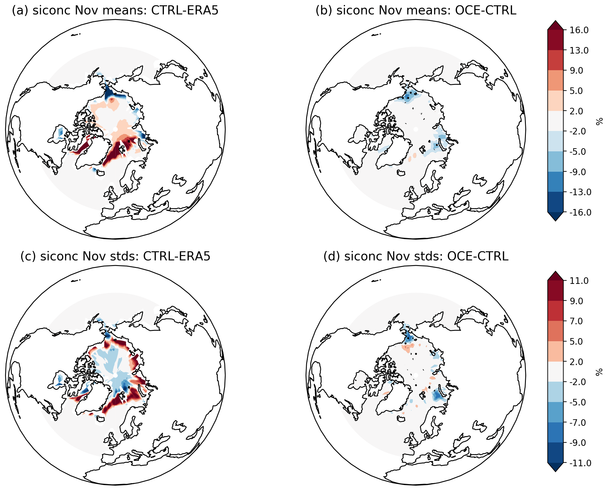
Figure 1 Sea ice concentration (mean and standard deviations) in November. Mean quantities in (a) CTRL − ERA5 and (b) OCE − CTRL. Standard deviations in (c) CTRL − ERA5 and (d) OCE − CTRL. Stippling in (b) and (d) highlights grid points where the change is statistically significant (p<0.05); in (a) and (c) almost every grid point outside the zero contour is significant, so stippling is not included for visual ease. The period considered is 1980–2015.

Figure 1 shows the differences in the mean and standard deviation of sea ice concentration (siconc) for CTRL vs. ERA5, as well as the impact on these differences in OCE. Note that this latter impact is visualized as the difference of OCE minus CTRL to more clearly highlight the changes. The differences are computed across 35 November months from the period 1 January 1980 to 31 December 2015: note that data are only drawn from the 35 winters spanning a full November–February season. A significant bias around the Greenland and Barents seas can be seen in the CTRL experiments, with the model producing too much sea ice with excessive interannual variability. The spatial pattern of the bias in the standard deviation, Fig. 1c, implies that this excess variability is due to a tendency for the ice edge to extend out much further in EC-Earth3 compared to ERA5. The main impact of OCE is to reduce the sea ice concentration along the ice edge and mitigate the excessive ice edge protrusion in the Barents Sea. This is consistent with the impact of the StoSIS in the coupled AWI-CM model (Juricke and Jung, 2014), suggesting that the changes here are mainly due to the sea ice perturbations promoting stronger ice motion towards the coast of Greenland and the Canadian Arctic Archipelago. This result is therefore consistent with their physical explanation of accelerated ice transport caused by an effective (non-linear) weakening of the sea ice by the random ice strength perturbations. Comparing Fig. 1b and d with a and c suggests that this is reducing the CTRL bias by around 10 % in the Labrador, Barents, and Kara seas but increasing the bias in the Bering sea. All these impacts were found to be qualitatively similar when considering the DJF period instead.

In summary, the OCE simulations appear to exhibit stochastically induced changes to ice transport which change the position, extension, and seasonal variability of the ice edge relative to CTRL. Such systematic changes to the variability are further supported by changes to the leading empirical orthogonal functions (EOFs) of sea ice concentration in OCE (not shown).

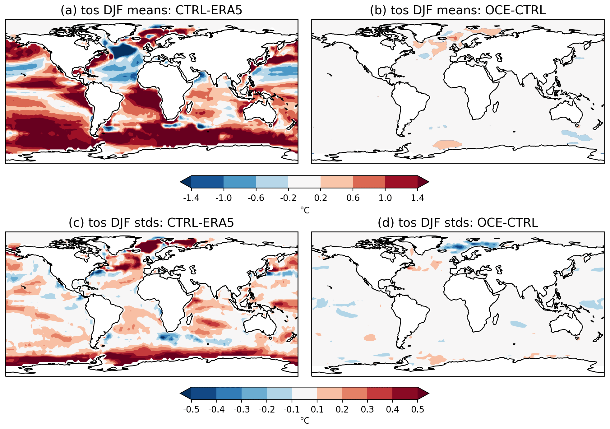
Figure 2 Sea surface temperature (mean and standard deviations) in DJF. Mean quantities in (a) CTRL − ERA5 and (b) OCE − CTRL. Standard deviations in (c) CTRL − ERA5 and (d) OCE − CTRL. In each plot, every grid point outside the zero contour is significant (p<0.05). The period considered is 1980–2015.

Figure 2 shows analogous differences in the mean and standard deviation of SSTs for CTRL vs. ERA5 and OCE. The only places where OCE appears to notably alter the mean state are the North Atlantic and Barents–Kara region. EC-Earth3 exhibits the common model bias of a cold North Atlantic (Wang et al., 2014), known to be associated with biases in the variability in and positioning of the Gulf Stream. The inclusion of stochasticity improves (i.e. increases) variability in the Gulf Stream, and this is a likely source of the differences in the North Atlantic mean state between CTRL and OCE, though it is clear that these changes do not generally constitute a reduction in the mean SST bias. Because there is a link between North Atlantic SSTs and the North Atlantic jet (Brayshaw et al., 2011; Keeley et al., 2012), we also show the impact on 850 hPa zonal winds in Fig. B1 of Appendix B. Interestingly, the changes to the jet more clearly constitute a bias reduction, which may suggest that these changes are not purely SST driven but rather related to the altered teleconnection discussed in the next section.

An examination of other variables supports an overall conclusion that the stochastic sea ice and ocean schemes are having only a modest impact on the climate mean state and do not, for example, alter the net surface global energy (not shown). We also found no evidence of significant changes to direct ocean–atmosphere coupling, as measured using the methods of Frankignoul et al. (1998) and von Storch (2000) (not shown); as will be seen later, changes to surface coupling do manifest in OCE but only in the presence of sea ice. It is likely that this limited impact on the climate mean state is due to the fact that the 1^∘ ocean does not permit eddies and is strongly damped by viscosity. Consequently, the stochastic ocean schemes, which are primarily attempting to perturb the variability in turbulent processes, cannot achieve much without making the perturbations extreme in magnitude (Juricke et al., 2017). This viewpoint is supported by the fact that in separate experiments using a 0.25^∘ ocean, the impact of the same schemes on SST variability was much greater (not shown). The main exception to this is in the Arctic and regions such as the North Atlantic, where, firstly, the sea ice perturbations play an active role, and, secondly, where the interplay between Gulf stream variability, atmosphere–ocean coupling, and vertical mixing in the ocean is large enough for the ocean perturbations to have a bigger impact.

4 Impact on the Arctic–NAO teleconnection

4.1 Changes to correlations and assessment of significance

Table 1 summarizes the magnitude of the teleconnection for each data set by showing the correlations between the November BKS ice concentration and the winter NAO over the period 1980–2015. Correlations significant to the 95 % threshold are shown in bold. It can be seen that ERA5 exhibits a significant positive correlation of ≈0.39, consistent with that reported by many other studies using a variety of techniques and observational data sets. None of the six individual CTRL members, nor the concatenated data set, show significant correlations, exhibiting both small positive and negative values. By contrast, every ensemble member of OCE shows a positive correlation. While only two of these attain statistical significance, after concatenation, OCE has a correlation of 0.26, which sits comfortably outside the 4σ range of the AR1 null hypothesis. The exact likelihood of this occurring under the null hypothesis was estimated to be less than 1 in 10 000.

Table 1 Correlations between anomalies in the November Barents–Kara sea ice concentration and the DJF NAO mean, over the period 1980–2015, for each data set. Subscript labels CTRL_n and OCE_n (N=35) denote ensemble members 1–6, while the entry for CTRL and OCE (N=210) uses the concatenated time series. Entries that are significant (p<0.05) are marked in bold. Significance is measured against a null hypothesis of uncorrelated, random AR1 processes.

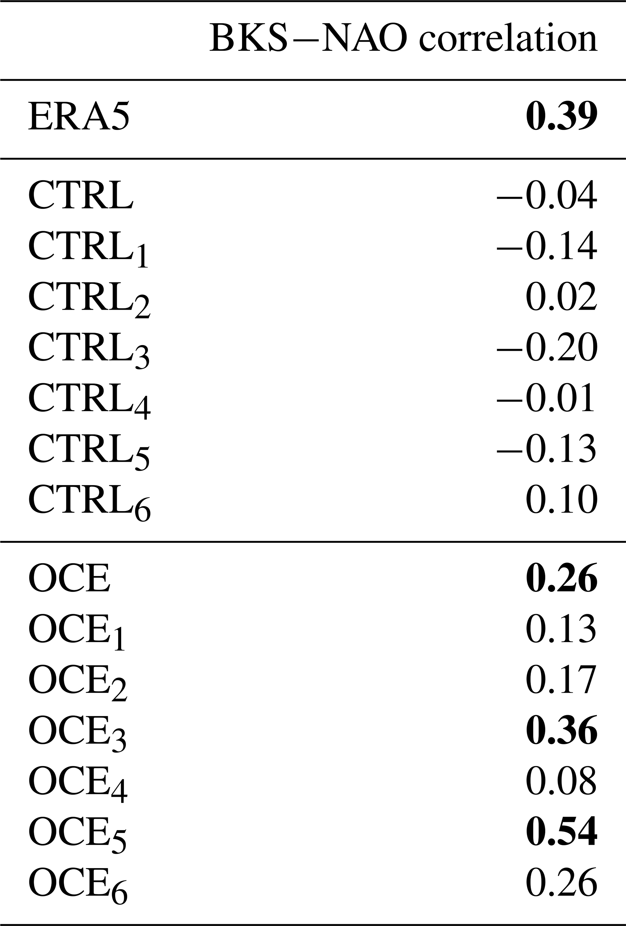
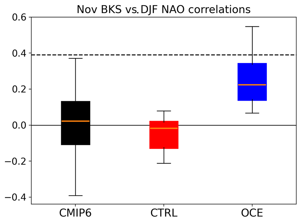
Figure 3 Boxplots of correlations between sea ice anomalies in the November Barents–Kara sea ice and the DJF NAO mean, over the period 1980–2015, for CMIP6 (black), CTRL (red), and OCE (blue). In each case, the box extends from the first to the third quartile of the data, with a line at the median. The whiskers extend from the box by 1.5 times the inter-quartile range. The stippled black line marks the correlation attained in ERA5.

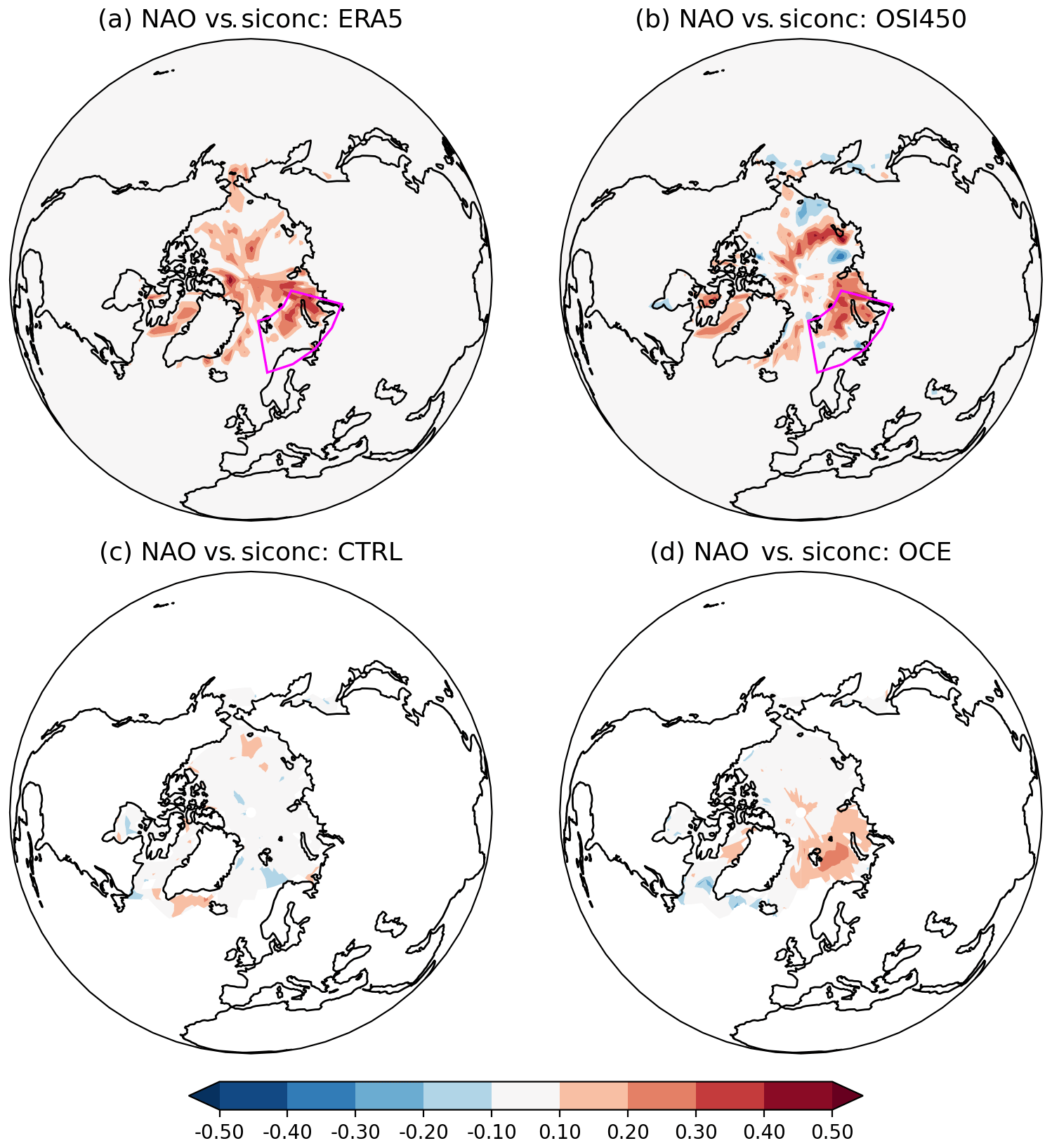
Figure 4 Correlations between the detrended November siconc anomalies at each grid point and the DJF NAO time series, over the period 1980–2015, in (a) ERA5, (b) OSI450, (c) CTRL, and (d) OCE. The ensemble members of the CTRL and OCE experiments have all been concatenated together. For the CTRL and OCE plots (c) and (d), every grid point outside the zero contour is statistically significant (p<0.05). For ERA5 and OSI450, only grid points in the Barents and Kara seas are significant. In (a) and (b) the Barents–Kara region has been marked by a purple box.

To visualize these changes, and place them in context, we show, in Fig. 3, box-and-whisker plots of these correlations along with those from the CMIP6 and HighResMIP simulations (referred to hereafter as just CMIP6 for simplicity). It is evident that the CMIP6 ensemble, consisting here of 70 model simulations covering the period 1980–2015, shows no consistent signal, with the distribution consistent with a null hypothesis that the correlations are just random draws from a mean zero normal distribution with a standard deviation of 0.17. The same conclusion holds if the HighResMIP simulations are excluded. The exact mean of 0.018 is slightly positive, consistent with earlier studies suggesting that models on the whole have a weak positive correlation, but the consensus is clearly weak, with around half the models showing negative correlations. We note that discrepancies with other studies showing a slightly stronger multi-model consensus may be due to the fact that we consider here a wider range of models than many studies, as well as the fact that different studies use differing experimental protocols that are not necessarily directly comparable (e.g. simulations using fixed anthropogenic forcing vs. simulations using actual historical forcings). The choice of which months to consider also differs between many studies. Nevertheless, it is visually clear that the deterministic CTRL correlations are consistent with random draws from the CMIP6 distribution and do not appear as unusually weak in the context we are interested in.

On the other hand, the OCE correlations are all positive with a mean value in the upper tercile of the CMIP6 distribution. The correlation of 0.54, obtained by one OCE ensemble member, is not obtained by any of the CMIP6 simulations we analysed. Under a null hypothesis that the correlations being considered are independent random draws around a Gaussian fit to the CMIP6 distribution, the chance of drawing six positive correlations is 0.5⁶≈0.016, i.e. 1.6 %. The chance of drawing six independent correlations that are not just positive but comparably large was estimated as being an order of magnitude less likely. In reality, the assumption that the six OCE ensemble members are strictly independent is likely false since, for example, we cannot rule out the possibility that being initialized in the same ocean state has predisposed the ensemble towards a particular pattern of decadal variability. However, since the CTRL members also start from the same state, the influence of the initialization on our results appears to be weak.

Figure 4 shows the spatial pattern of the correlations in each data set by plotting correlations of the DJF NAO time series against November sea ice concentration at every grid point in the Arctic. As expected, CTRL shows only a few spurious-looking correlations, with no significant correlations in the BKS region. For OCE, the largest correlations are found in the Barents Sea, but significant correlations are also found in the Kara Sea. The fact that the correlations in the Kara Sea in OCE are weaker than those in ERA5 may be related to the sea ice biases shown in Fig. 1.

In summary, we conclude that the correlations obtained in the OCE ensemble are significantly larger than both those in CMIP6 and CTRL. In particular, the circulation in OCE appears to exhibit a robust ice–NAO teleconnection.

4.2 Decadal variability, trends, and climate change

While the focus of this paper is on the period 1980–2015, we make some remarks on decadal variability in the teleconnection and the possible influence of trends, which may be of interest for future work. The reader is warned that, in the absence of more detailed analysis, this discussion is necessarily somewhat speculative.

We find that all the simulations appear to be initialized into a period of weak, but broadly positive, BKS–NAO correlations, with no clear difference between CTRL and OCE (not shown). The two ensembles diverge from each other around 1975 so that by 1980 the correlations of OCE are robustly separated from those of CTRL, as discussed in the preceding section. It is likely that some of this variability is a result of random internal variability, but consideration of the spatial pattern of the correlations suggests a somewhat more nuanced picture. This can be seen by plotting the equivalent of Fig. 4 for earlier periods: see Fig. B2 for an example of this for the period 1950–1985. This shows that in this earlier period, the weak, positive BKS–NAO correlations in CTRL and OCE are driven by a weak signal from the Barents Sea. More striking however is the presence of a much larger signal emanating from the Greenland and Labrador seas in both ensembles. Further analysis (not shown) suggests that the region of significant grid point correlations shrinks over time: in CTRL, the region basically shrinks to nothing by 1975, while in OCE it shrinks to Barents and Kara (Fig. 4).

It seems likely that this behaviour is at least in part due to the sea ice loss that occurs in this time period. Both models lose a considerable amount of sea ice in the Greenland, Barents, and Kara seas, with the OCE model losing somewhat less in Barents and Greenland and somewhat more in Kara. The loss of sea ice in the Greenland Sea in particular is associated with a permanent retreat of the sea ice edge, resulting in a collapse of interannual sea ice variability, and hence correlations, in this region.

Several studies have made the point that the strongest heat flux anomalies are associated with the variability in the ice edge. The strong temperature gradients between the relatively warm ocean and the cold atmosphere aloft mean that variations in the extent of the ice edge are associated with heat flux anomalies reaching as high as 500 W m⁻²​​​​​​​: see, for example, Koenigk et al. (2009) for a comprehensive overview. The fact that it is these heat flux anomalies that are hypothesized to influence the circulation, as opposed to the sea ice per se, suggests a plausible physical justification for the teleconnection being associated with the region of maximum November ice edge variability. For observational data in the modern period, this corresponds to the Barents and Kara seas, particularly the Barents Sea (Deser et al., 2000; Vinje, 2001; Koenigk et al., 2009). However, given the significant changes to the ice edge over the 20th century, it is interesting to consider whether other regions, such as the Greenland Sea, played an important role in the past. Figure B3 shows that, indeed, in the OCE ensemble, the November sea ice variability in the Labrador and Greenland seas is much higher in the period 1950–1980 and also that there is almost no variability in the Kara Sea in this period. The same is true for the CTRL ensemble (not shown). We note that in Kelleher and Screen (2018), it was shown that there is a significant influence of winter Greenland sea ice area on the winter polar cap geopotential height anomalies in pre-industrial CMIP5 simulations, corroborating the potential importance of the Greenland Sea in the past.

To summarize, we find that the trend of a shrinking ice edge appears to influence the location of significant grid point correlations and that much of the decadal variability in the BKS–NAO correlation prior to 1980 can be accounted for by the fact that other regions, particularly the Greenland Sea, appear to be more important in earlier periods. It is noteworthy that even in these earlier periods, the OCE ensemble has significantly higher correlations than CTRL in the relevant regions (see Fig. B2), suggesting that the stochastic perturbations are consistently enhancing ice–NAO teleconnections across the full period 1950–2015.

A final point of interest is that both CTRL and OCE show entirely comparable negative trends of the NAO over 1950–2015 (not shown). It is therefore possible that the stochastic schemes are having a negligible impact on the long-term climate change response to sea ice loss in EC-Earth3 since differing responses might be expected to manifest as differing NAO trends. It would be interesting to run future projections of the CTRL and OCE configurations to assess this further. As far as future changes to interannual variability are concerned, the discussion on decadal variability above is consistent with the trivial observation that the teleconnection would be expected to slowly vanish as the ice edge retreats.

4.3 Tropospheric vs. stratospheric pathways

Figure 5 shows the vertical structure of the teleconnection, measured by regressing November BKS ice against zonally averaged DJF zonal winds, at different latitudes and pressure levels. Two things are apparent from this. Firstly, the teleconnection in OCE, viewed here as a northward shift of the jet in response to a positive BKS anomaly, extends all the way up to the stratosphere. This means that both tropospheric and stratospheric pathways may be present in the teleconnection seen in OCE. We do not attempt to disentangle the two at present but remind the reader that the stochastic perturbations in OCE are strictly limited to the ocean and ice at the surface, so it is unlikely that changes to the teleconnection are a result of direct changes to the stratospheric dynamics. Secondly, the teleconnection in OCE is still weaker than that of ERA5: while the correlations are comparable in magnitude, the actual regression coefficients are larger in ERA5 and are statistically significant across the entire vertical structure. The same picture holds if regressing against zonally averaged geopotential height anomalies instead (not shown).

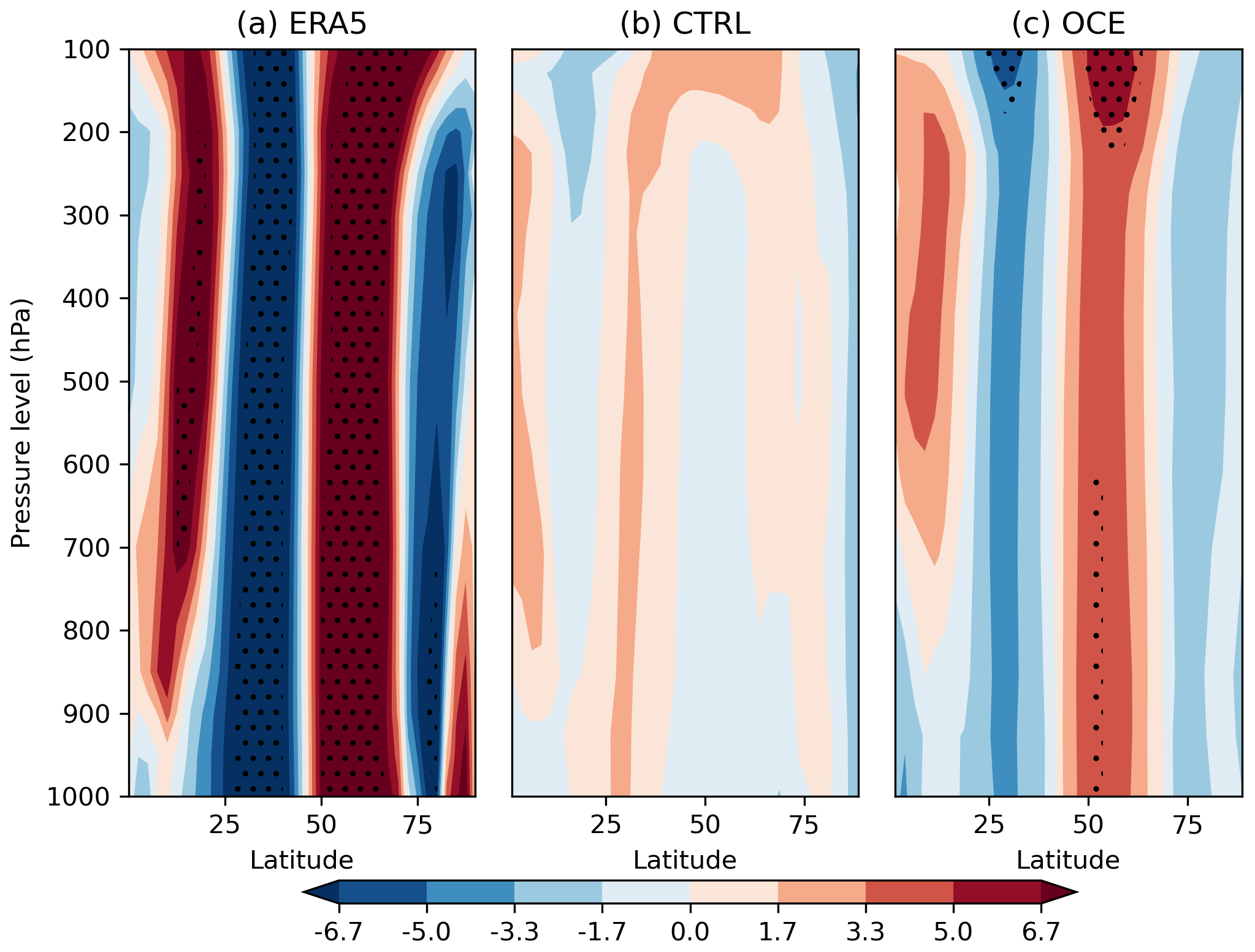
Figure 5 Regression coefficients of November BKS sea ice against zonally averaged DJF zonal winds at various latitudes (degrees north) and pressure levels (hPa) in (a) ERA5, (b) CTRL, and (c) OCE. The period considered is 1980–2015. Stippling highlights grid points where the associated correlation coefficient is statistically significant (p<0.05).

5 A quantitative explanation via ice–ocean–atmosphere coupling

5.1 Mean state changes alone do not suffice

In Sect. 3 it was shown that the stochastic schemes have notably changed the mean state of North Atlantic SSTs and Arctic sea ice. An obvious first hypothesis is therefore that the improved teleconnection is the result of these changes. To test this, we examined an equivalent set of three deterministic ensemble members using prescribed observational SST and ice boundary forcing from the HadISST data set, which we refer to as the AMIP ensemble. The equivalent version of Fig. 4 for AMIP (Fig. B4), obtained by correlating the model’s NAO with the prescribed sea ice at each grid point, shows no indication of any ice–NAO link at any grid point. The correlations of the November BKS sea ice anomalies and the DJF NAO, for each of the three ensemble members, are 0.18, 0.01, and −0.05: the correlation using the concatenated time series is 0.06. None of these values are significantly different from 0, and considering other 35-year periods between 1950 and 2015 does not change this. We therefore conclude that the AMIP ensemble does not exhibit an ice–NAO teleconnection.

Note that the tendency for AMIP-style models to have weaker Arctic–mid-latitude teleconnections than their coupled counterparts has been noted in both a multi-model context (Blackport and Screen, 2021) and for EC-Earth3 in particular (Caian et al., 2018). Consequently, having a perfect ice and/or ocean mean state does not necessarily produce a realistic teleconnection.

5.2 Coupled ice–NAO dynamics and the LIM model

In the previous section we saw that prescribing observed ocean and sea ice forcing does not result in the deterministic model exhibiting a significant teleconnection. If internal atmospheric variability is playing a key role in generating the teleconnection, then prescribing the sea ice may act to obfuscate this (Blackport and Screen, 2021). However, another possibility is that an important role is being played by the dynamic coupling of the atmosphere, ocean and ice. The potential importance of coupling to simulate the circulation or surface response associated with Arctic sea ice anomalies was already emphasized in Strong et al. (2009) and Strong and Magnusdottir (2011), as well as more recently in Deser et al. (2016), Mori et al. (2019a), and Mori et al. (2019b).

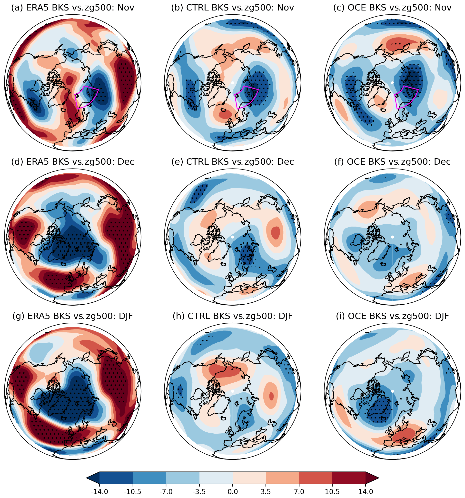
Figure 6 Regression coefficients of November BKS sea ice anomalies against monthly zg500 grid point anomalies in ERA5 for (a) November, (d) December, and (g) DJF. The same for CTRL and OCE in (b), (e), and (h) and (c), (f), and (i), respectively. The period considered is 1980–2015. Stippling highlights grid points where the associated correlation coefficient is statistically significant (p<0.05).

To gain additional insight into this, we first examine the temporal evolution of the teleconnection. This is done in Fig. 6, which shows the regression coefficients of November BKS sea ice anomalies against monthly zg500 anomalies in November, December, and DJF for ERA5, CTRL, and OCE.

The instantaneous November regression coefficients, Fig. 6a, b, and c, are all fairly similar in all three data sets, with a tripole pattern formed by a low over the Kara Sea, a high near Greenland, and a low near the eastern coast of North America. The pattern projects weakly onto the negative NAO in the Euro-Atlantic sector but deviates from the canonical NAO pattern over Greenland and the Arctic region by comparison with Fig. 6g, which shows the full DJF NAO response in ERA5. This November tripole pattern will be capturing the combined effects of the atmospheric forcing on the ice, as well as the forcing of the ice on the atmosphere, but appears to be most consistent with atmospheric forcing in the form a northerly flow into the Barents Sea², promoting enhanced sea ice (Koenigk et al., 2009). In the following months, both ERA5 and OCE see this tripole evolve into a larger low centred on Greenland, with a broad high across the North Atlantic and Europe; in DJF this pattern clearly corresponds to a positive NAO for both. In CTRL, on the other hand, the same evolution never takes place, and the seasonal evolution simply consists of a slow dissipation of the initial anomaly. Similar plots showing the evolution of heat flux and temperature anomalies (Figs. B5 and B6) corroborate this story, with a similar initial anomaly that evolves relatively realistically over time in OCE but simply persists or peters out in CTRL.

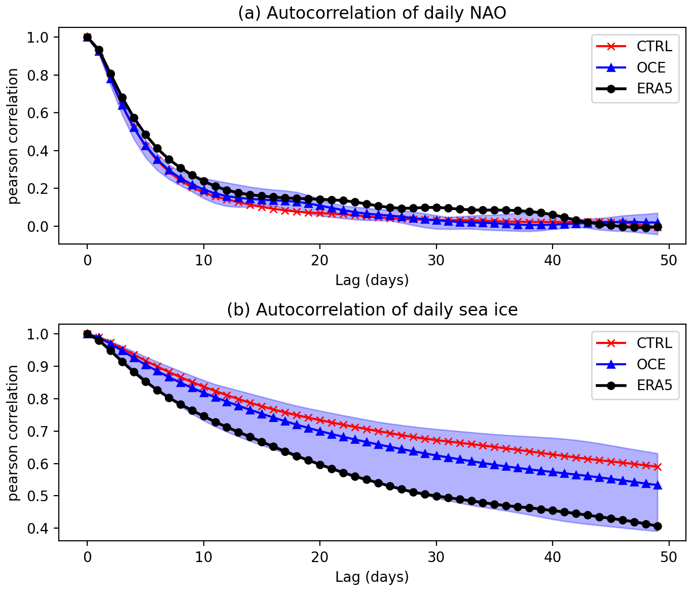
Figure 7 Autocorrelation of (a) the daily NAO and (b) the daily BKS sea ice for ERA5 (black dots), CTRL (red crosses), and OCE (blue triangles). Data are restricted to days in November through February, 1980–2015. Shading indicates the ensemble spread of OCE: the CTRL spread (not shown) is similar in extent.

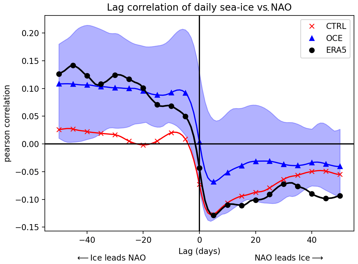
Figure 8 Lagged correlations of the daily NAO against the daily BKS sea ice for ERA5 (black dots), CTRL (red crosses), and OCE (blue triangles). Negative lags correspond to sea ice forcing the NAO, and vice versa for positive lags. Correlations are computed using all days in November through February, 1980–2015. Shading indicates the ensemble spread of OCE: the CTRL spread (not shown) is similar in extent. Note that only every fifth point has been marked by a symbol for visual clarity.

The ability of OCE to evolve the same initial response better than CTRL might be plausibly attributed to changes in persistence, either of the NAO or the sea ice. However, since the atmospheric component is identical in OCE and CTRL, there is no obvious mechanism for how the persistence of the NAO might change, and the lack of a teleconnection when prescribing the sea ice rules out the persistence timescales of the sea ice alone from explaining the change. Figure 7 confirms that the daily autocorrelation of the NAO has not changed notably between OCE and CTRL. Both ensembles have much higher sea ice persistence than ERA5, but again, the difference between OCE and CTRL is small by comparison. By contrast, Fig. 8 shows a marked difference between OCE and CTRL in the lag correlation. Most notably, the OCE model appears to be considerably more realistic when the sea ice leads the NAO, with CTRL showing virtually no impact of sea ice on the NAO for lags of up to 50 d ahead. When the NAO leads the ice, CTRL appears more realistic for small lags, but the difference has largely vanished by lags of a month or more.

Note that the opposite sign of the lag correlation based on whether the ice or the NAO is leading has been reported previously in both model data (Magnusdottir et al., 2004) and observational data (Strong et al., 2009), and it suggests a natural physical interpretation of the coupling (Strong et al., 2009). A positive sea ice anomaly in the BKS region (i.e. an extension of the sea ice edge) leads to a reduced local heat flux into the atmosphere. This reduced heat flux then forces the positive phase of the NAO, via some combination of Rossby wave forcing, changes to the meridional temperature gradient, and stratospheric pathways. This corresponds to a northward shift of the eddy-driven jet (Woollings et al., 2010), which would lead to anomalous wind stress along the ice edge and a consequent reduction in the initial positive sea ice anomaly. The more northerly jet may also lead to shifts in the distribution of sea ice more broadly which are potentially important for supporting a realistic evolution of the initial atmospheric response.

In light of our results so far, it is natural to ask if the changes to short timescale coupling between the ice and the NAO can account for the changes in the seasonal timescale teleconnection. To test this, we model the ice–NAO system using the following pair of coupled ordinary differential equations:

$$\begin{array}{}\text{(1)}& {\displaystyle \frac{\mathrm{d}}{\mathrm{d}t}}\mathrm{NAO}=a\cdot \mathrm{NAO}+b\cdot \mathrm{ICE}+{\mathit{\xi }}_{\mathrm{NAO}},\text{(2)}& {\displaystyle \frac{\mathrm{d}}{\mathrm{d}t}}\mathrm{ICE}=c\cdot \mathrm{NAO}+d\cdot \mathrm{ICE}+{\mathit{\xi }}_{\mathrm{ICE}}.\end{array}$$

Here NAO is just the daily NAO index, and ICE is the daily sea ice anomaly in the BKS region. The coefficients a and d are capturing the presence of autocorrelation, while the coefficients b and c capture the presence of coupling; the ξ terms in both equations represent the residual forcing on both quantities and are assumed to be random Gaussian processes with no temporal autocorrelation and a mean of 0. This model, hereafter referred to as the LIM, has been used extensively in the literature to capture coupling between variables in climate data, such as atmosphere–ocean coupling, and the coefficients and noise terms can be estimated using linear inverse modelling (see, for example, Penland and Sardeshmukh, 1995; Penland and Magorian, 1993; Alexander et al., 2008; Hawkins and Sutton, 2009; Newman et al., 2009, for some examples). A brief summary of how to do this is included in Appendix A: the reader may consult Penland and Sardeshmukh (1995) for more details. We are not aware of earlier examples in the literature applying the LIM framework to ice–atmosphere coupling, though the approach of Strong et al. (2009) and Strong and Magnusdottir (2011) is closely related.

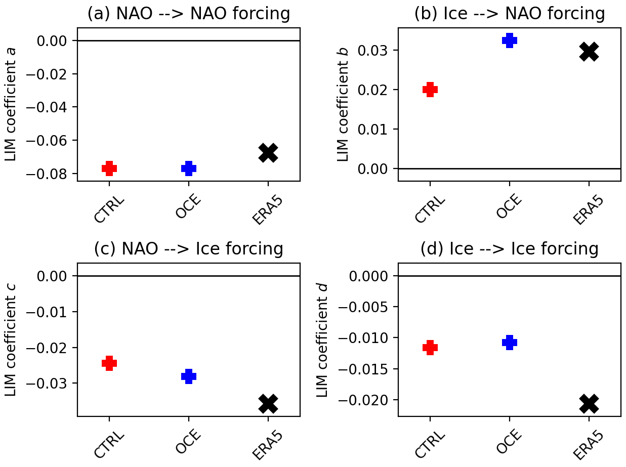
Figure 9 Estimated coefficients of the LIM model, as described by Eqs. (1) and (2). In (a), the coefficient a, describing the forcing of the NAO on itself 1 d later, (b) the coefficient b, describing the forcing of sea ice on the NAO 1 d later, (c) the coefficient c, describing the forcing of the NAO on sea ice 1 d later, and (d) the coefficient d, describing the forcing of sea ice on itself 1 d later. CTRL and OCE data are marked in red and blue, respectively. ERA5 is shown with a black cross. Daily data covering November–February, 1980–2015, are used.

5.3 Validation of the LIM hypothesis

Figure 9 shows the estimated LIM coefficients for ERA5 (black), CTRL (red), and OCE (blue), where daily data spanning November through February (NDJF) of 1980–2015 have been used. Fitting the LIM requires a choice of a lag, and we used the simplest possible choice of 1 d, which essentially amounts to fitting the full seasonal ice–NAO dynamics to the 1 d​​​​​​​ dynamics. Studies such as Deser et al. (2007) suggest that it may take up to a few weeks for sea ice anomalies to project onto the NAO, so it may in principle be better to use a longer lag. However, within the range of lags for which the LIM hypothesis is a good fit, the model parameters are independent of the specific choice of lag (Penland and Magorian, 1993). Nevertheless, due to the high autocorrelation of both the ice and the NAO, it is possible that correlations on daily timescales are reflecting dynamical processes taking place on longer (e.g. weekly) timescales. When carrying out the fitting to CTRL and OCE, all ensemble members were used under the assumption that the extent of coupling should in theory be identical across different ensemble members. Because the estimated coefficients are inevitably influenced by the chaotic internal variability, using all ensemble members (rather than fitting to each member separately) also gives more robust estimates.

Once these coefficients and the November initial conditions for each data set are obtained, it is straightforward to generate random reconstructions of the daily NDJF data using the LIM by feeding in the ice and NAO anomalies on the 1 November for each year as initial conditions and integrating the system (see Appendix A for details). Examples of LIM-reconstructed DJF NAO time series can be seen in Fig. B7, which also illustrates that, by construction, the reconstructed time series have on average the same variance as the true time series. These reconstructions can then be used to validate the LIM hypothesis for ERA5, CTRL, and OCE by testing if the ice–NAO correlations of each data set are indistinguishable from the ice–NAO correlations of randomly drawn LIM reconstructions. To test this, we generated, for each data set, 1000 random reconstructions of the corresponding LIM and for each of these correlated the LIM November ice with the LIM DJF NAO. For ERA5, this produced a mean correlation of 0.27 with a 95 % confidence interval of −0.05 to 0.56; for OCE, a mean correlation of 0.36 and a confidence interval of 0.06 to 0.62; and for CTRL, a mean correlation of 0.26 and a confidence interval of −0.08 to 0.55. Three things can be inferred from these distributions. Firstly, by comparison with Table 1, the teleconnection correlations in ERA5 and those from the OCE ensemble are consistent with the distribution obtained from their respective LIM, suggesting that the behaviour of ERA5 and OCE is consistent with the LIM hypothesis. Secondly, the correlations in the actual CTRL ensemble are not consistent with the LIM distribution, being clustered down at the lower end of the distribution with three of the six members falling outside the 95 % confidence interval (see Table 1). In other words, the behaviour of CTRL is not consistent with the LIM hypothesis. Thirdly, the variation across the LIM coefficients (Fig. 9) is largely immaterial for generating significant positive correlations. In particular, the reason the CTRL model fails to have a significant ice–NAO teleconnection cannot be accounted for by, for example, the smaller b coefficient compared to ERA5 and OCE. Rather, it is that the LIM hypothesis as a whole fails in the case of CTRL (see further discussion in Sect. 5.4).

By more systematically varying the LIM coefficients (not shown), we found that significant positive correlations are generated in the LIM primarily from the non-zero forcing of the ice on the NAO and the long persistence of sea ice anomalies: this persistence means that the small daily timescale forcing accumulates into a larger forcing on seasonal timescales. The forcing of the NAO on the ice has a mostly negligible effect on the magnitude of the correlation. The exact values of the parameters, including the forcing from the NAO, are on the other hand crucial for obtaining reconstructions with the correct variance. If the NAO forcing term is suppressed, then the LIM DJF NAO is considerably larger in magnitude than the true DJF NAO of the given data set. In other words, the sea ice forcing being continuously damped by the NAO is what allows the LIM reconstructions to have a variance closely matching that observed, but because correlations are insensitive to magnitudes, this does not impact the ice–NAO correlations generated by the LIM.

Finally, we note that no meaningful difference was found between the noise terms of the LIM for CTRL and OCE.

5.4 Why has the coupling improved in the stochastic ensemble?

The conclusion of the previous section was that the LIM hypothesis is reasonable for both ERA5 and OCE but fails in the case of CTRL. This suggests that the relevant ice–ocean–atmosphere coupling is not simulated correctly in CTRL and is improved by the inclusion of stochasticity. Why is this the case? The LIM hypothesis is, in essence, that the winter ice–NAO link can be inferred from the initial conditions on 1 November and how the ice and NAO are linked on daily timescales. There are three obvious ways this might fail for CTRL: (1) the initial conditions are unrealistic in CTRL, (2) the daily timescale link itself is unrealistic in CTRL, and (3) the dynamical response to the initial conditions, as it evolves over the winter season according to the daily timescale link, is being systematically disrupted somehow in CTRL.

Concerning the first possibility, we find no meaningful difference between the initial ice and NAO conditions of CTRL vs. OCE: see Fig. B8. While Fig. 1 shows that there are some localized differences in the variability across the BKS region, the total variance of the 1 November ice across the region as a whole is almost identical for both ensembles. There is no significant difference between the NAO variances of the two ensembles either. It does not therefore seem likely that differences in the initial conditions are playing an important role.

Concerning the second possibility, since the ice–NAO link is mediated via heat fluxes, it is natural to consider if the heat flux response in CTRL is somehow deficient compared to ERA5 and OCE. As a first test, we find no evidence that the BKS-averaged heat flux response to a sea ice anomaly on 1 November is significantly different in the CTRL or OCE ensemble means, including the vertical extent of the response. This is already apparent from Figs. 6, B5, and B6, which show that the mean November signal looks roughly similar in CTRL and OCE. However, more subtle differences between the two ensembles are apparent in Fig. 10, which shows lagged correlations between daily heat fluxes and daily BKS sea ice. While the ensemble mean correlations are similar for CTRL and OCE at all lags, the CTRL ensemble shows a much wider ensemble spread than OCE. This is especially notable for positive lags, i.e. when heat fluxes lead the ice. For lags of 5 d​​​​​​​ or less, ERA5 shows a clear positive correlation: an increase in upwards heat flux³ removes heat from the surface, leading to an increase in sea ice. In OCE, all ensemble members show positive correlations for these lags, but for CTRL the response is almost equally likely to have the wrong sign. This suggests that, counter-intuitively, the inclusion of stochastic perturbations causes the sea ice response to be more tightly constrained. In fact, this increased stability of the ice and heat flux relationship is apparent at all lags in Fig. 10 and is also found when restricting the data to other regions than BKS (not shown), pointing towards a more consistently realistic surface coupling in OCE. This may plausibly contribute to a more consistent interannual ice–NAO link and hence larger correlations.

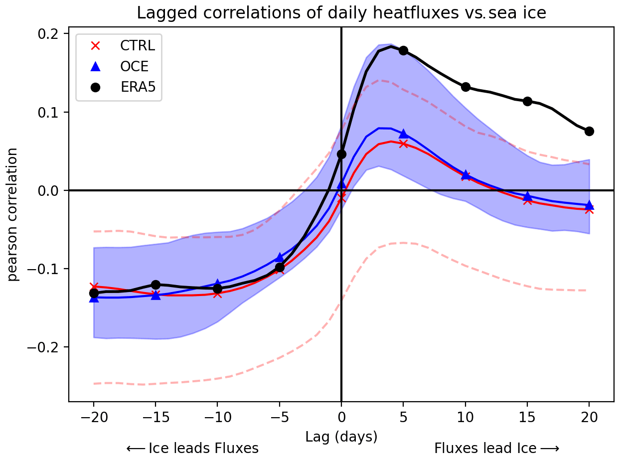
Figure 10 Lagged correlations of the daily BKS heat fluxes against daily BKS sea ice for ERA5 (black dots), CTRL (red crosses), and OCE (blue triangles). Negative lags correspond to the ice forcing heat fluxes, and vice versa for positive lags. Note that positive heat flux values correspond to an upwards flux. Correlations are computed using all days in November through February, 1980–2015. Blue shading indicates the ensemble spread of OCE; the CTRL spread is indicated by stippled red lines. Note that only every fifth point has been marked by a symbol for visual clarity.

Finally, concerning the third possibility, we suggest two ways in which the evolution of the initial pressure anomaly might be systematically disrupted in CTRL. Firstly, a northward shift of the jet (i.e. a positive NAO) will act to adjust the entire sea ice edge, not just that of Barents and Kara (Koenigk et al., 2009). The SSTs, crucial for generating heat flux anomalies and likely reinforcing the anomaly through ocean–atmosphere coupling (Deser et al., 2016), will also be adjusted by wind stress across the North Atlantic as a whole. These non-local responses may be crucial for the correct evolution of the initial pressure anomaly: such adjustments would not be captured by the AMIP simulations, potentially also explaining why these fail to exhibit a teleconnection. As discussed in the preceding paragraph, Fig. 10 suggests that such remote ice and/or SST adjustments, necessarily mediated via heat fluxes, might be better simulated in OCE. Figure B5 shows a difference in the heat flux response around the Labrador and Greenland seas in December between ERA5 and OCE and CTRL, and we speculate that adjustments in these regions may be important. Secondly, it may be that some other unrealistic atmospheric forcing occurring later in the winter is destructively interfering with the ice–NAO link in CTRL. There is some indication that the CTRL ensemble exhibits an unrealistically strong teleconnection between El Niño–Southern Oscillation (ENSO) and the NAO (see Fig. B9) which is alleviated in OCE: because the sign of this ENSO link is the opposite of the ice–NAO link, this may be a source of such destructive interference. The fact that deterministic models can have overly dominant ENSO teleconnections that are alleviated with the inclusion of stochasticity was also noted in Strommen et al. (2017).

Other more complex ice–ocean–atmosphere interactions, such as those discussed in Caian et al. (2018), might also be done poorly in CTRL, and it would be interesting to apply their methods here. In addition, it cannot be ruled out that the mean position of the storm track needs to be well aligned with the ice edge in order to foster the growth of the initial anomaly (Deser et al., 2007), implying that the mean state changes between CTRL, OCE, and AMIP may be important as well. Note that the AMIP simulations, while having perfect SSTs and ice, still have biases in their simulated storm track which could prevent a robust teleconnection from emerging.

It is clear that more work is required to understand the mechanisms at play, which we hope to address in the future. Nevertheless, our analysis suggests that the improved teleconnection in OCE may be a combination of improved ice–ocean–atmosphere coupling and mean state changes.

6 Discussion and conclusions

We briefly summarize the results of our analysis.

• The inclusion of stochasticity to the ocean and sea ice components of EC-Earth3, as evaluated with the OCE ensemble experiments, leads to the emergence of a statistically significant teleconnection between November Barents–Kara sea ice and the DJF NAO, comparable to, but somewhat weaker than, that observed in ERA5. No such teleconnection is present in the deterministic EC-Earth3 (the CTRL ensemble; Table 1 and Fig. 3). The teleconnection signal in OCE extends all the way up to the stratosphere (Fig. 5).

• Comparison with the CMIP6 and CTRL ensemble suggests that the odds of generating six random OCE ensemble members which, by chance, all show a consistent ice–NAO teleconnection is extremely low (Fig. 3). This implies that the teleconnection is likely a real feature of the circulation in OCE.

• An AMIP-style ensemble of deterministic simulations with prescribed sea ice and SSTs is still not able to manifest an ice–NAO teleconnection, suggesting that the relevant model biases are related to coupling at the surface (Fig. B4).

• Analysis using lag correlations and a simple LIM model suggests that the teleconnections in ERA5 and OCE can be accounted for by the hypothesis that the direct, local coupling between the sea ice and the NAO on daily timescales completely captures the seasonal dynamics but that this hypothesis fails in the case of CTRL (Fig. 8 and Sect. 5.3). This suggests that the ice–ocean–atmosphere coupling of EC-Earth3 has been improved by the inclusion of the stochastic schemes.

• Two broad hypotheses are put forward for the improved ice–NAO coupling in OCE: (1) a more realistic relationship between heat fluxes and sea ice (Fig. 10) and (2) a systematic disruption of the BKS-induced pressure anomaly in CTRL by some other unrealistic atmospheric variability, such as an overly dominant ENSO (Fig. B9). Improvements to the mean ice state (Fig. 1) and zonal winds (Fig. B1) may also be playing a role.

These results have important implications for the study of Arctic–mid-latitude teleconnections. The potential importance of realistic sea ice–ocean–atmosphere coupling in generating an ice–NAO teleconnection has previously been highlighted by Strong et al. (2009). The possible role of inadequate surface coupling in models has more recently been highlighted by Mori et al. (2019a) in the context of surface level teleconnections; Mori et al. (2019b) also emphasized the role of poorly simulated sea ice variability in models. Our work adds further evidence to these views by explicitly demonstrating how model development aimed at improving ice and ocean variability, here in the form of stochastic process representation, resulted in the emergence of a robust teleconnection in a model which did not previously exhibit one. Our analysis supports the hypothesis that improvements to ice–ocean–atmosphere coupling are playing an important role in this result, and it furthermore makes it clear that one cannot expect, a priori, that a given climate model does have realistic coupling. Thus, inadequate coupling may be behind coupled runs exhibiting a wide spread in ice–NAO correlations spanning both positive and negative correlations (Koenigk and Brodeau, 2017; Siew et al., 2021), as well as the weak correlations found when averaging over multiple ensemble members or longer simulation periods (Blackport and Screen, 2021; Siew et al., 2021). It is also possible that the signal-to-noise paradox in seasonal forecasting is partially due to such biases.

While the most direct interpretation of our analysis seems to be that stochasticity has altered the surface coupling, it is plausible that mean state changes are also playing a role. This is due to the potential sensitivity of the sea ice signal to a favourable storm track, which implies that getting the right signal may depend on the combined sea ice, ocean, and atmospheric mean state. As such, the lack of a teleconnection in the AMIP experiments does not conclusively rule out that the mean state changes in OCE (Sect. 3) are important. The analysis of lagged correlations and the LIM model lend support to the role of coupling, but it might be that the ice edge of OCE is more optimally aligned with the storm track compared to in CTRL and that the changes seen in Figs. 8 and 9 are simply reflecting this. Untangling this would require more careful analysis of targeted experiments which fall outside the scope of this paper.

If the stochastic schemes are, in fact, improving the coupling between sea ice, ocean, and the atmosphere, what is the precise mechanism which makes the perturbations have this impact? Here too, more careful analysis would be required which goes beyond the scope of this paper. However, a simple conceptual hypothesis might be the following. The evolution of the deterministic sea ice, including how it responds to atmospheric forcing, may be biased in various ways. Years when the sea ice forces the NAO may depend sensitively not just on the initial sea ice anomaly but also on wider adjustments to Arctic sea ice and North Atlantic SSTs following the initial atmospheric response. The deterministic model may simply be doing these adjustments incorrectly a lot of the time (as hinted at by Fig. 10), with the role of stochasticity being to force the model to not always do the same thing. We note that this idea of stochasticity acting as “damage mitigation” against biased deterministic models is ubiquitous in weather forecasting (Palmer et al., 2009; Berner et al., 2017). That the stochastic sea ice scheme can lead to very different mean responses for Arctic sea ice due to the coupling response with the atmosphere has been shown by Juricke and Jung (2014) with dedicated full and one-way coupling experiments. We consider it likely that the stochastic sea ice scheme is the dominant factor for changes to the sea ice–NAO teleconnection seen here, but note that the study of Juricke et al. (2018) has shown that the stochastic ocean schemes can also lead to improved skill over North America in seasonal forecasts, a teleconnection effect they relate to improved ocean–atmosphere coupling. It may also be that interactions between the ice and ocean schemes are essential. Further ensemble experiments would be required in order to test the impact of each scheme separately.

Our analysis has some important limitations. For example, we cannot exclude the possibility that the experiments we considered are biased in some way, e.g. due to the initial ocean state predisposing OCE towards certain patterns of decadal variability associated with higher ice–NAO correlations. Another clear limitation is that the impact of these stochastic schemes on Arctic teleconnections has only been tested using a single climate model and may not produce similar effects in other models. Indeed, it is well known that the same stochastic scheme can have different impacts on different models (Strommen et al., 2019). There may also be important non-linear effects such as those discussed in Caian et al. (2018). Finally, we made no attempt to separate the tropospheric and stratospheric pathways. On the other hand, we note that the stochastic schemes were introduced precisely to improve variability and coupling (Juricke et al., 2013; Juricke and Jung, 2014; Juricke et al., 2014, 2017), so there is good reason a priori to expect such changes to manifest in experimental data.

Our results, which suggest that the inclusion of a stochastic component in the sea ice and ocean can alleviate model biases, in coupling, the mean state, and variability, add to an increasingly large body of work showing that stochasticity can be beneficial in models across all timescales. It is especially noteworthy that although changes to the mean and variability of the model due to stochasticity in this study may, in some regions, be rather moderate, other important physical mechanisms in the climate system, such as teleconnections, might be better represented with the stochastic schemes. While the use of stochasticity in the atmospheric component is becoming more widespread, its inclusion in other components of the model is still novel. The potential benefits of representing uncertainty in all major components of a climate model was first raised in Palmer (2012), and our paper adds further weight to this view.

Appendix A: Linear inverse modelling

A system of coupled ordinary differential equations, defined by equations (1) and (2), is used to describe coupled ice–NAO interactions on daily timescales. The parameters are fitted using standard methods of linear inverse modelling. Detailed descriptions of how to do this in full generality can be found in Penland and Magorian (1993) and Penland and Sardeshmukh (1995), but to aid the reader we briefly outline the computational steps. Let $\mathbf{B}=\left(\begin{array}{cc}a& b\\ c& d\end{array}\right)$ be the coefficient matrix, and let x be the vector made up of the daily time series of the NAO and ICE. To estimate B in terms of daily timescale coupling, we computed the lag-0 covariance matrix C₀ and the lag-1 covariance matrix C₁ of x. The matrix B was then estimated as the matrix logarithm $\mathbf{B}=\log \left({\mathbf{C}}_{\mathrm{1}}{\mathbf{C}}_{\mathrm{0}}^{-\mathrm{1}}\right)$. The noise terms can then be estimated by computing the eigenvectors and values of the “noise matrix” $\mathbf{Q}=-\mathrm{1}\cdot ({\mathbf{BC}}_{\mathrm{0}}+{\mathbf{C}}_{\mathrm{0}}{\mathbf{B}}^T)$.

Once the parameters have been fitted in this way for a given data set, a reconstruction of a daily DJF NAO time series can then be created, for a given year, by initializing the coupled system with the NAO and ICE anomalies of 1 November of that year and integrating the defining equations forward in time. A single November through February period is therefore just a 120 day integration from the initial conditions.

Appendix B: Additional material

We​​​​​​​ include some figures and tables left out of the main text.

Table B1 CMIP6 models used in this paper.

Table B2 HighResMIP models used in this paper.

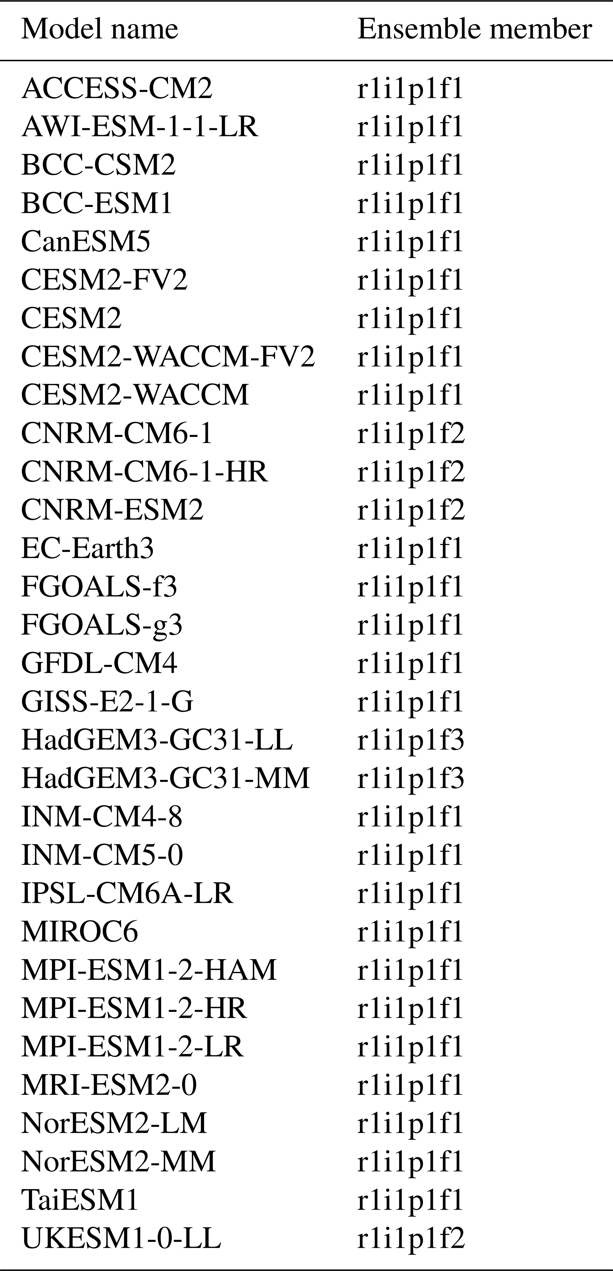
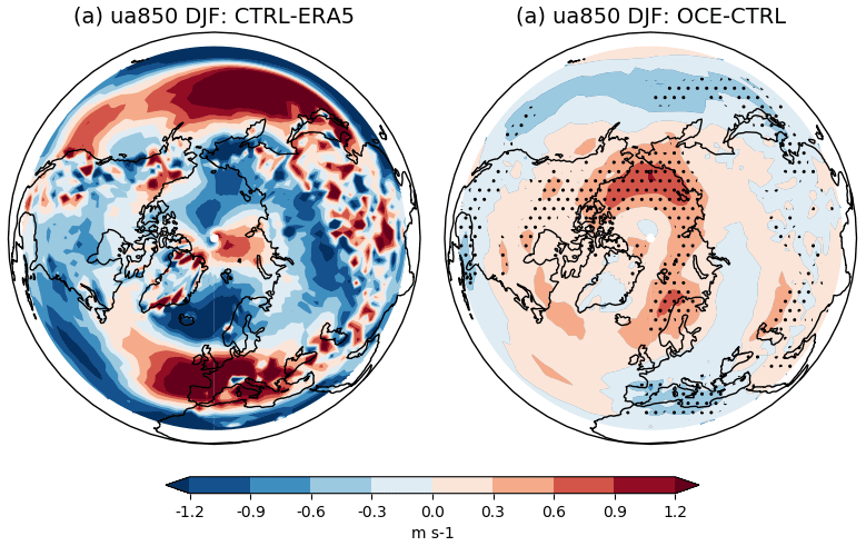
Figure B1 Mean zonal winds at 850 hPa (ua850) over the DJF season. In (a) CTRL minus ERA5, and (b) OCE minus CTRL. Stippling highlights grid points where the change is statistically significant (p<0.05); in (a) most points outside the zero contour are significant, so stippling is not included for visual ease. The period covered is 1980–2015.

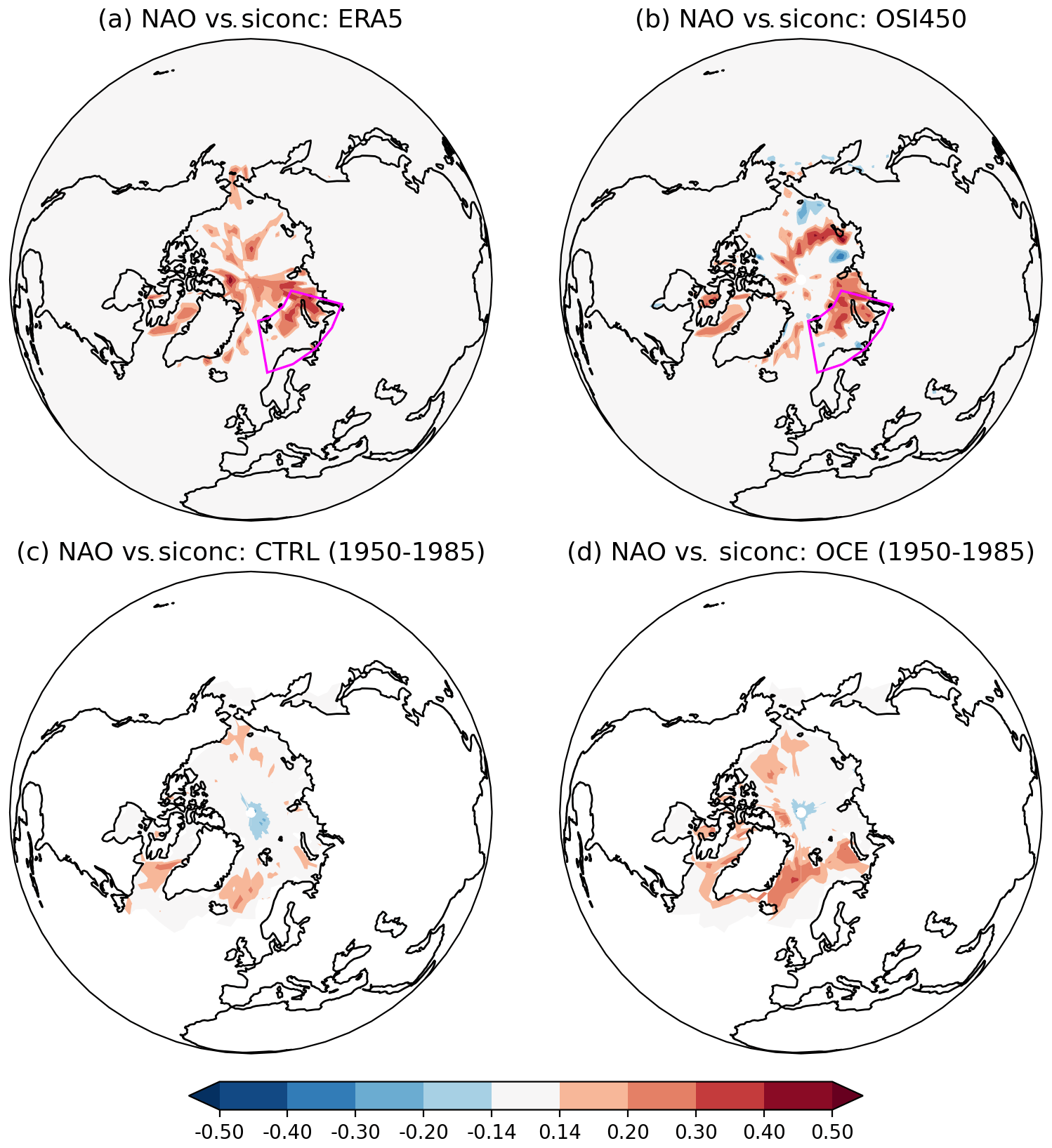
Figure B2 Correlations between the detrended November siconc anomalies at each grid point and the DJF NAO time series. In (a) ERA5 (1980–2015), (b) OSI450 (1980–2015), (c) CTRL (1950–1985), and (d) OCE (1950–1985). The ensemble members of the CTRL and OCE experiments have all been concatenated together. For the CTRL and OCE plots (c) and (d), every grid point outside the zero contour is statistically significant (p<0.05). For ERA5 and OSI450, only grid points in the Barents and Kara seas are significant. In (a) and (b) the Barents–Kara region has been marked by a purple box.

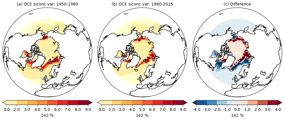
Figure B3 Sea ice concentration variance in November. In (a) the OCE ensemble over the period 1950–1980, (b) the OCE ensemble over the period 1980–2015, and (c) the difference of (b) minus (a).

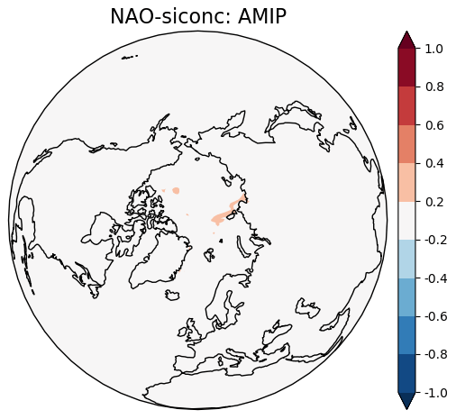
Figure B4 Correlations between the detrended November siconc anomalies at each grid point and the DJF NAO time series, using the AMIP ensemble. All three members have been concatenated. The period covered is 1980–2015.

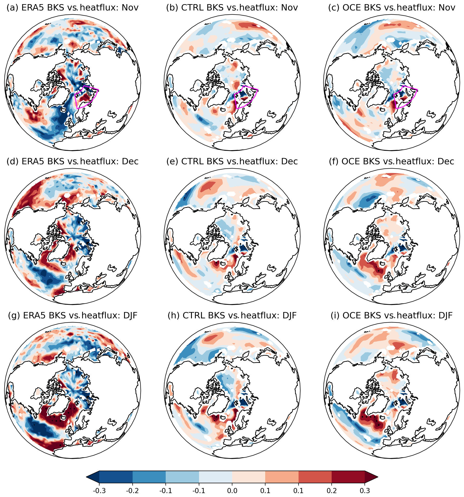
Figure B5 Regression coefficients of November BKS sea ice anomalies against monthly heat flux grid point anomalies in ERA5 for (a) November, (d) December, and (g) DJF. The same for CTRL and OCE in (b), (e), and (h) and (c), (f), and (i), respectively. The period considered is 1980–2015. Stippling highlights grid points where the associated correlation coefficient is statistically significant (p<0.05). The Barents–Kara region is shown with a purple box.

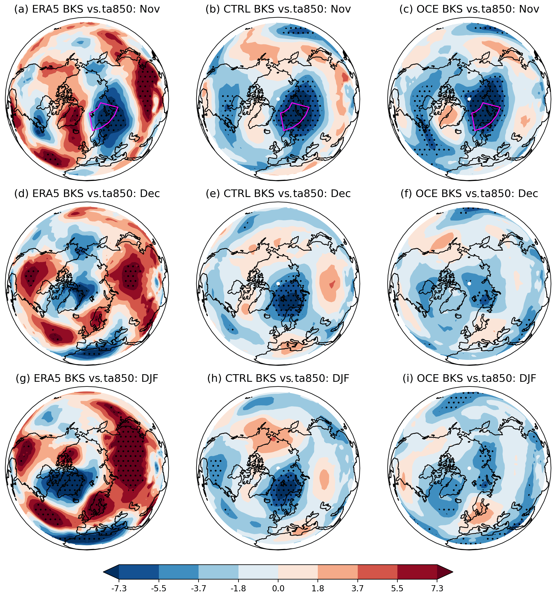
Figure B6 Regression coefficients of November BKS sea ice anomalies against monthly 850 hPa temperature (ta850) anomalies at each grid point in ERA5 for (a) November, (d) December, and (g) DJF. The same for CTRL and OCE in (b), (e), and (h) and (c), (f), and (i), respectively. The period considered is 1980–2015. Stippling highlights grid points where the associated correlation coefficient is statistically significant (p<0.05). The Barents–Kara region is shown with a purple box.

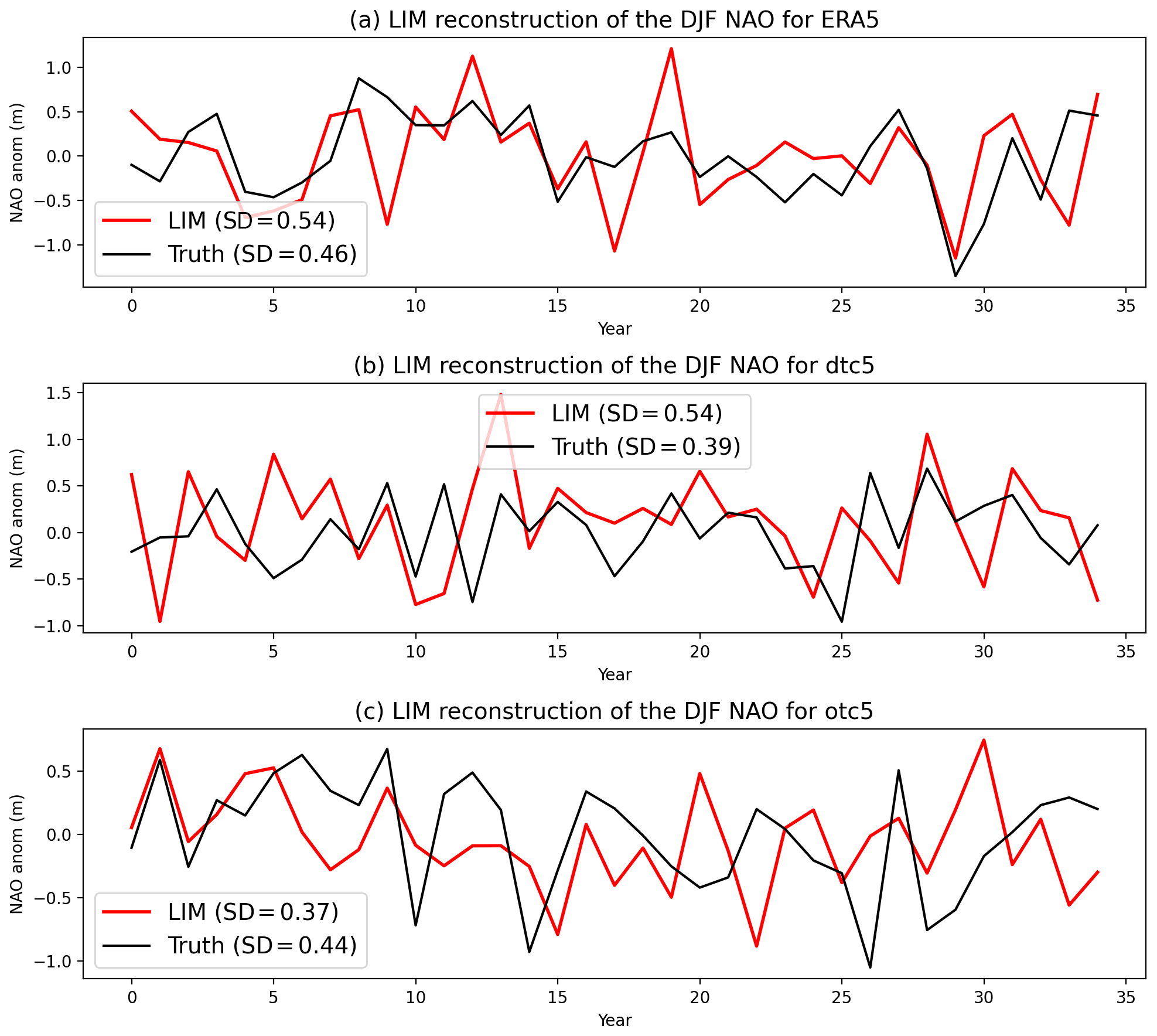
Figure B7 Randomly generated reconstructions of the DJF NAO time series using the LIM initialized each 1 November for the years 1980 to 2015. For (a) ERA5, (b) the fifth ensemble member of CTRL, and (c) the fifth member of OCE. In each plot, the LIM reconstruction is in red and the true time series in black. The sample standard deviations of each time series have been noted in the legends. Reconstructions of other ensemble members of CTRL and OCE are qualitatively similar.

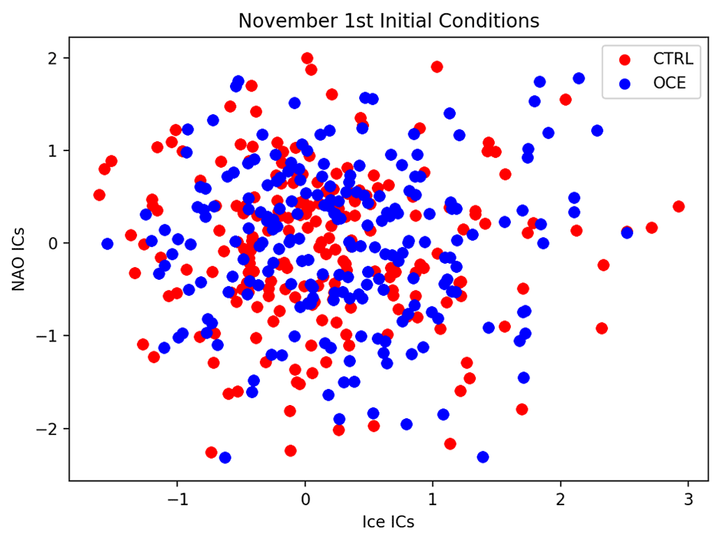
Figure B8 Scatter plot of the ice and NAO initial conditions, i.e. the values of the BKS sea ice (x axis) and NAO anomalies (y axis) on 1 November, for every year between 1980 and 2015. In red: CTRL; in blue: OCE.

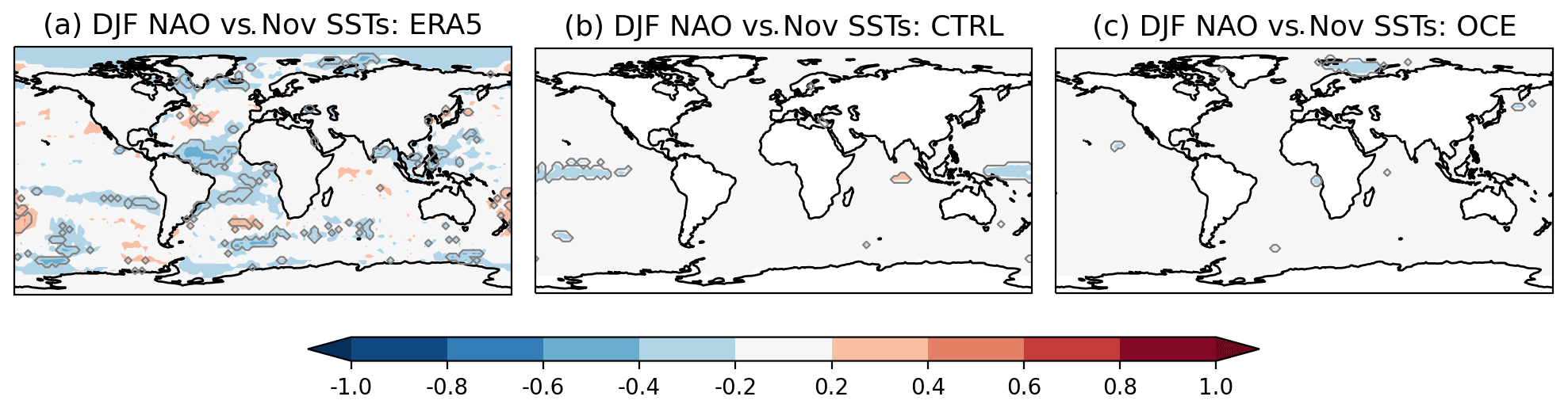
Figure B9 Correlations between detrended November SSTs at each grid point and the DJF NAO time series for (a) ERA5, (b) CTRL, and (c) OCE. The ensemble members of the CTRL and OCE experiments have been concatenated together. The period covered is 1980–2015. The grey contour highlights statistically significant correlations (p<0.05).