Validation of boreal summer tropical–extratropical causal links in seasonal forecasts

Much of the forecast skill in the mid-latitudes on seasonal timescales originates from deep convection in the tropical belt. For boreal summer, such tropical–extratropical teleconnections are less well understood compared to winter. Here we validate the representation of boreal summer tropical–extratropical teleconnections in a general circulation model in comparison with observational data. To characterise variability between tropical convective activity and mid-latitude circulation, we identify the South Asian monsoon (SAM)–circumglobal teleconnection (CGT) pattern and the western North Pacific summer monsoon (WNPSM)–North Pacific high (NPH) pairs as the leading modes of tropical–extratropical coupled variability in both reanalysis (ERA5) and seasonal forecast (SEAS5) data. We calculate causal maps based on the Peter and Clark momentary conditional independence (PCMCI) causal discovery algorithm, which identifies causal links in a 2D field, to show the causal effect of each of these patterns on circulation and convection in the Northern Hemisphere. The spatial patterns and signs of the causal links in SEAS5 closely resemble those seen in ERA5, independent of the initialisation date of SEAS5. By performing a subsampling experiment (over time), we analyse the strengths of causal links in SEAS5 and show that they are qualitatively weaker than those in ERA5. We identify those regions for which SEAS5 data well reproduce ERA5 values, e.g. the southeastern USA, and highlight those where the bias is more prominent, e.g. North Africa and in general tropical regions. We demonstrate that different El Niño–Southern Oscillation phases have only a marginal effect on the strength of these links. Finally, we discuss the potential role of model mean-state biases in explaining differences between SEAS5 and ERA5 causal links.

1 Introduction

Seasonal forecasts provide a useful tool to study atmospheric dynamics and predict seasonal variations in wind, rainfall and temperature patterns across tropical and extratropical regions (Bauer et al., 2015; Palmer and Anderson, 1994). To a certain extent, seasonal forecasts can be used by stakeholders and governments to anticipate and mitigate extreme weather events, failures in crop yields or water scarcity hazards for infrastructure such as electricity grids (Lazo et al., 2009; Challinor et al., 2003; Hagger et al., 2018; Meza et al., 2008). Tropical–extratropical interactions are linked to mid-latitude boreal surface weather conditions and represent a source of predictability at seasonal and subseasonal timescales (Shukla, 1998). Hence, improving the representation of these teleconnections in seasonal forecasts can help to improve our knowledge of atmospheric dynamics as well as to better forecast relevant weather patterns to support early warning systems.

Obtaining reliable seasonal forecasts is a challenging problem due to the intrinsic nonlinearity of processes governing atmospheric motions (Holton, 1973). While providing weather forecasts beyond a 2-week threshold is a complex problem due to the chaotic nature of atmospheric processes (Tsonis and Elsner, 1989; Palmer and Anderson, 1994), slowly varying climatic fields such as sea surface temperatures (SSTs) and soil moisture can provide forecast skill beyond the weekly timescale (Charney and Shukla, 1981). The representation of the interaction of the atmosphere with other components of the climate system, e.g. via SST variability, is an important requirement to achieve forecast skill (Roberts et al., 2021; Tietsche et al., 2020). Historically, both statistical (Gadgil et al., 2005; Kumar, 2012) and dynamical approaches (Jain et al., 2018; Scaife et al., 2019) have been used to provide seasonal forecasts, often with comparable skill (Seo et al., 2009; Barnston et al., 1999). However, when the focus is on the representation of physical processes rather than the forecast skill, dynamical forecasts, generated by general circulation models (GCMs), provide a more complete representation of the atmospheric physics that governs weather and climate behaviour (Shukla et al., 2000). Dynamical seasonal forecasts explicitly solve dynamic and thermodynamic equations and are better suited for representing the dynamic and thermodynamic processes and emerging dynamical teleconnections within the climate system.

To produce accurate seasonal forecasts, GCMs need to represent the physical processes operating at those timescales truthfully in the current climate. Great progress in this field has been made in recent decades, leading to an improved representation of dynamic and thermodynamic processes and a steady increase in model resolution (Bauer et al., 2015; Palmer, 2017; Haarsma et al., 2016). Nevertheless, probabilistic reliability of dynamical seasonal forecasts remains limited (Weisheimer and Palmer, 2014). In this context, analysing seasonal forecasts such as the SEAS5 (Johnson et al., 2019) dataset provided by the European Centre for Medium-range Weather Forecasts (ECMWF), can help to identify, understand and improve biases between observations and model simulations.

Tropical–extratropical interactions in the Northern Hemisphere during boreal summer have been analysed in several recent studies (O'Reilly et al., 2018; Di Capua et al., 2020a; Ding et al., 2011). Heat generated by tropical convective activity provides a source of wave activity that can affect weather in the mid-latitudes (O'Reilly et al., 2018; Rodwell and Hoskins, 1996; Ding and Wang, 2005), while in turn mid-latitude wave activity can modulate rainfall events in the tropical belt (Ding and Wang, 2007; Di Capua et al., 2020b). Here, we focus on the two main modes of covariability between tropical convection and mid-latitude circulation as identified in Di Capua et al. (2020a) and Ding et al. (2011). The first mode of covariability is represented by the circumglobal teleconnection (CGT) paired with the South Asian monsoon (SAM) convection (Ding et al., 2011; Di Capua et al., 2020a). Circumglobal wave trains such as the CGT are connected to temperature and precipitation anomalies at intraseasonal and interannual timescales in the northern mid-latitudes (Ding and Wang, 2005; Di Capua et al., 2020b). Recent work based on statistically evaluating causal relationships in reanalysis data has shown that the CGT pattern and the SAM circulation system are connected by a two-way causal interaction (Di Capua et al., 2020b). Moreover, the causal effect of each of these patterns on atmospheric circulation and surface conditions can be effectively represented on a 2D map (Di Capua et al., 2020a). The CGT has been studied in seasonal forecasts provided by ECMWF, and the corresponding results show that generally the model can reproduce this pattern (Beverley et al., 2019). However, the CGT pattern in seasonal forecasts is too weak, likely due to a misrepresentation of the SAM convective activity in the tropical belt.

The second mode of covariability between tropical convection and boreal summer circulation is represented by a pair of patterns associated with the western North Pacific summer monsoon (WNPSM) and the North Pacific high (NPH) (Di Capua et al., 2020a). The NPH is the result of the northward displacement of the North Pacific subtropical high due to the onset of the WNPSM activity at the beginning of July (Di Capua et al., 2020a). In reanalyses, the influence of these two patterns on other atmospheric fields is weak compared to the SAM–CGT pair and mostly confined to the Pacific Ocean. Nevertheless, the WNPSM and NPH systems can affect typhoon cyclogenesis in the tropical Pacific (Briegel and Frank, 1997) and temperature and circulation patterns in eastern Asia and North America, respectively, potentially acting as a source of wave activity downstream (Di Capua et al., 2020a; Ding et al., 2011). Therefore, even though the direct area of influence of the WNPSM–NPH pair is found over the ocean, effects of changes in their intraseasonal variability are relevant to remote and highly populated areas (e.g. the US west coast or Japan).

Causal discovery algorithms, such as the Peter and Clark momentary conditional independence (PCMCI) method, help overcome issues with commonly used statistical techniques, like correlation measures. When carefully applied, they allow one to identify and separate true causal from spurious links (Runge, 2018; Runge et al., 2014, 2019). PCMCI has been used to study stratospheric polar vortex variability (Kretschmer et al., 2017, 2016, 2018), the Silk Road pattern interdecadal variability (Stephan et al., 2019), Atlantic hurricane activity (Pfleiderer et al., 2020), and causal interactions between the Indian summer monsoon and mid-latitude wave trains (Di Capua et al., 2020a, b). Moreover, PCMCI has also proven useful in providing early forecasts of Moroccan crop yields (Lehmann et al., 2020), subseasonal statistical forecasts of US surface temperatures (Vijverberg and Coumou, 2022; Vijverberg et al., 2020) and statistical seasonal predictions of Indian summer monsoon rainfall (Di Capua et al., 2019).

Process-based validation can help us to understand and correct biases in seasonal forecasts (Eyring et al., 2019; Horak et al., 2021). Here, we propose to use causal discovery to perform a process-based validation (Nowack et al., 2020) of tropical–extratropical interactions in SEAS5 seasonal forecasts. We compare observed (i.e. reanalysis) causal interactions between tropical convective activity and mid-latitude wave trains in the Northern Hemisphere during boreal summer with those present in seasonal forecasts. The scope of this comparison is three-fold: (i) we validate causal links in a coupled GCM in forecasting mode against those derived from observations, and (ii) we gather information on missing or misrepresented links in the GCM in forecast mode. Finally, (iii) we analyse whether these differences can be attributed to model biases and what impact different phases of the El Niño–Southern Oscillation (ENSO), present in the initial conditions of the forecasts, have on the strength and representation of causal links. Thus, this work represents an initial step to improving forecast skill and the representation of tropical–extratropical teleconnections in GCMs.

The remainder of this paper is organised as follows: Sect. 2 presents the data and methods used. Section 3 describes the results obtained by applying causal maps first to ERA5 reanalysis and then SEAS5 data. Section 4 provides a discussion of the obtained results in the context of the existing literature and the final conclusions.

2 Data and methods

2.1 Data

We analyse intraseasonal (weekly) tropical convective activity and mid-latitude circulation characteristics during the extended boreal summer period (May to September, MJJAS) using gridded data (0.25^∘ × 0.25^∘ upscaled to 2^∘ × 2^∘) from the ERA5 reanalysis dataset (Hersbach et al., 2020) and the SEAS5 seasonal retrospective forecast dataset (Johnson et al., 2019), both provided by the European Centre for Medium-range Weather Forecasts (ECMWF). From the ERA5 dataset, we use daily (temporally averaged to obtain weekly samples) geopotential height fields at 200 hPa (Z200), outgoing long-wave radiation (OLR), sea surface temperature (SST) and zonal (U200) wind fields for the period 1979–2020 (ERA-L) and for the subset 1993–2016 (ERA-S) (to be consistent with the available SEAS5 dates). While Z200 is useful for representing the mid-latitude circulation, OLR can be used as a proxy of tropical convective activity. Despite SEAS5 providing values for precipitation globally, we prefer using OLR instead of precipitation itself as precipitation is not assimilated in the reanalysis (and thus is less reliable than assimilated fields such as SST), observational precipitation data coverage for tropical regions is sparse and to keep this analysis consistent with Di Capua et al. (2020a). For the general circulation model comparison, we analyse OLR, Z200, SST and U200 fields for the period 1993–2016 of SEAS5. As for ERA5, SEAS5 data are also regridded from the original 1^∘ × 1^∘ onto a 2^∘ × 2^∘ grid, and daily data are temporally averaged to obtain weekly samples. The interannual variability, seasonal cycle and any long-term trend are removed. To do so, first the interannual variability, i.e. the average value of each May-to-September period, is subtracted from the corresponding year (thus ensuring that the weekly signal does not include the interannual variability). Then, for each of the 21 time steps considered in each MJJAS season, the trend over the 24 years is removed and anomalies around zero are calculated, thus removing both the trend and seasonal cycle.

While reanalysis data from ERA5 provide one realisation per year, SEAS5 provides 25 ensemble members each year, thus a total of 25×24 (600) model years. A schematic of the SEAS5 ensemble is shown in Fig. 1. Considering only the summer season (June to September) plus May, as required by the causal discovery framework to ensure a proper handling of time lags (see Sect. 2.3), we have a total of 21 weeks per extended summer (MJJAS) for each year (Fig. 1a). Thus, for the common period 1993–2016, we have a total of $\mathrm{21}\times \mathrm{24}=\mathrm{504}$ weekly time samples for ERA5 and $\mathrm{21}\times \mathrm{24}\times \mathrm{25}=\mathrm{12}\mathrm{600}$ time samples for SEAS5 (Fig. 1b). Note that, for both ERA5 and SEAS5 datasets, the first week of the MJJAS period starts on 7 May (the first full week common to both datasets when for ERA5 the first week of the year starts on 1 January).

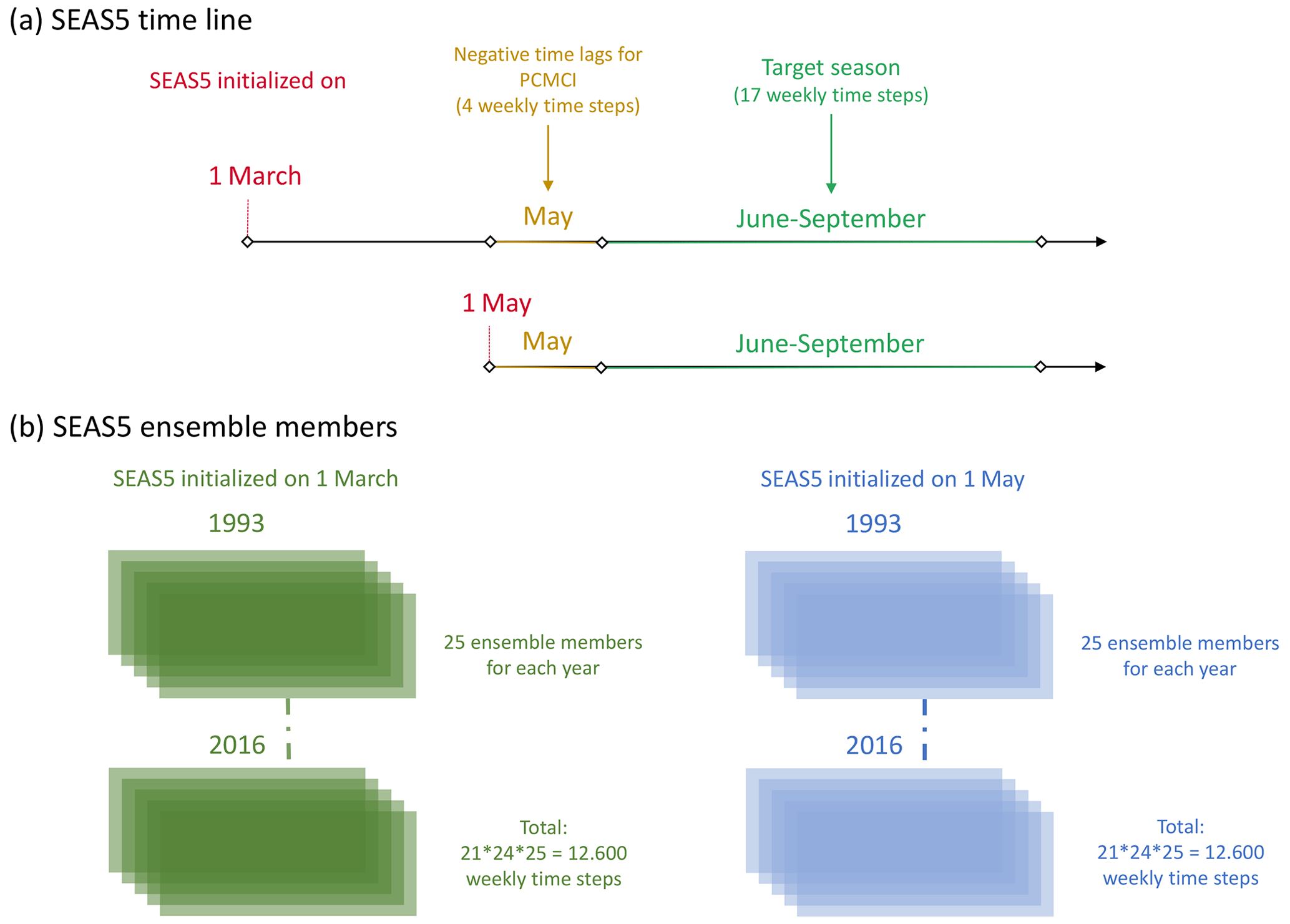
Figure 1 Schematic representation of the SEAS5 forecasting set-up. Panel (a) shows the time line for SEAS5 initialisation and target period. Panel (b) shows a schematic of the SEAS5 ensemble members.

Treating the 25 ensemble members per year for 24 years as one unique time series of 600 years composed of distinct subsequences is possible under the assumption that each member of each ensemble year is independent of the remaining members. While the ensemble is generated by varying the initial conditions, this assumption of uniqueness is not true in general, since each ensemble member for a given year has common lower boundary conditions for the atmosphere, inherited from slowly evolving features in the ocean, e.g. SST anomalies in the tropics and extratropics. However, for the purpose of this analysis we are interested in the relative effect of a certain (set of) variable(s) on the remaining atmospheric fields inside the intraseasonal variability, with a maximum lag of a few weeks (thus on a much shorter timescale than interannual). It must be noted that we do not intend to use SEAS5 data to assess or exploit its forecast skill but instead to assess the ability of a general circulation model in forecasting mode at reproducing observed tropical–extratropical teleconnections. In other words, whether there is shared information between two ensemble members for a certain year (e.g. whether a certain phenomenon in the analysed climate system is stronger or weaker) or whether a specific year shows better forecast skill than another does not affect the relative effect of that phenomenon on some selected atmospheric fields. However, we cannot exclude that different initialisation dates (SEAS5 seasonal forecasts are initialised on the first day of each month and run for 7 months), and the vicinity of the target season to the beginning of the simulation may influence the outcome and the resulting causal links. Thus, we choose to analyse SEAS5 forecasts initialised on both 1 March and 1 May of each year, with a target season of June–September (see Fig. 1a). This way, the model has up to 3 (and at least 1) months of spin-up to reduce the influence of the initial conditions. However, for the forecasts initialised on 1 May, although the month of May is outside the target season, May time steps enter the set of precursors (see below) for June time steps. Thus, we provide a sensitivity analysis to show which results depend on (or are independent of) the chosen initialisation date. In the final step of this work, we will assess whether the effect of ENSO on wind fields and convective activity in the Northern Hemisphere (i) is sufficiently well reproduced in SEAS5 when compared to ERA5 and (ii) influences the identified tropical–extratropical causal links.

2.2 Modes of co-variability

To identify the dominant modes of intraseasonal co-variability between tropical convective activity and mid-latitude circulation in the Northern Hemisphere, we apply maximum covariance analysis (MCA) as described in Di Capua et al. (2020a). The first two MCA modes are calculated by applying MCA to OLR fields in the tropical belt (15^∘ S–30^∘ N, 0–360^∘ E) paired with Z200 fields in the northern mid-latitudes (25–75^∘ N, 0–360^∘ E), thus using the same geographical borders as in Di Capua et al. (2020a).

By construction, the first MCA mode explains a maximum of squared covariance between the selected two fields (Ding et al., 2011; Wiedermann et al., 2017), and MCA modes are ranked according to their explained squared covariance fraction (SCF) (Wilks, 2011). With this method, it is possible to identify pairs of patterns that can explain shared covariance and (to some extent) evolve simultaneously. However, shared covariance, as in general correlation-based techniques, does not imply causality. To check whether these patterns may be causally related (e.g. via dynamical mechanisms), we apply the PCMCI causal discovery algorithm (see Sect. 2.3).

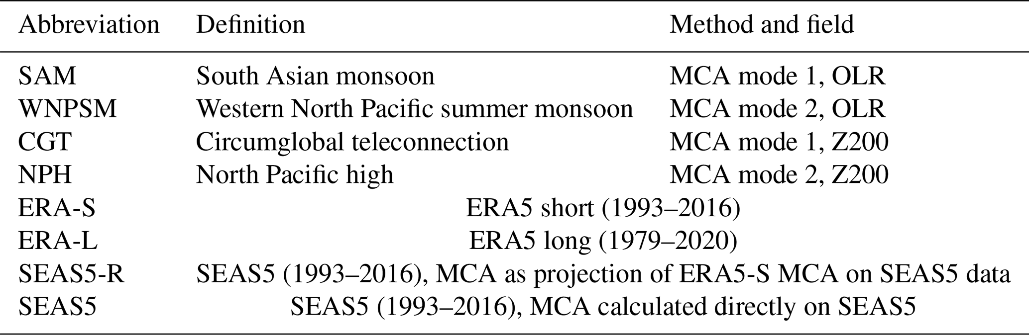
Each MCA mode provides two coupled (2D) spatial patterns (one for tropical OLR and one for mid-latitude Z200) and two associated time series. Note that separate time series are created for the OLR and Z200 MCA patterns and for each MCA mode and a total of four time series when MCA modes 1 and 2 are analysed. These time series are obtained by projecting each (2D) MCA spatial pattern on the corresponding time-varying atmospheric field and represent the time-dependent MCA scores or pattern amplitudes for both fields. Each time series describes the magnitude (prominence) and phase (sign) of those patterns for each time step of the field's time series. The abbreviations associated with the MCA patterns are shown in Table 1.

Table 1 List of the main abbreviations used in the article.

Here, we apply MCA both to the full 1979–2020 (ERA-L) and reduced 1993–2016 (ERA-S) periods and to SEAS5 for the period 1993–2016. On the one hand, we attempt to be consistent with the available SEAS5 data (ERA-S). On the other hand, we want to provide a direct comparison with Di Capua et al. (2020a), who studied the previous ERA-Interim reanalysis product, by exploiting the full length of the time series (ERA-L). However, the first two MCA modes calculated with SEAS5 data do not provide a close enough representation of the patterns shown in ERA5 (see spatial correlation coefficients shown in Table 2 and Sect. 3.1). Thus, to provide a meaningful comparison between the two datasets, we define MCA patterns in SEAS5 by projecting the first two ERA5 MCA patterns onto SEAS5 data and referring to these modes as MCA SEAS5-R. This is done in the same way in which the ERA5 MCA scores/time series are calculated, i.e. by calculating the dot product of each ERA5 MCA mode with the corresponding OLR or Z200 field time series for each time step.

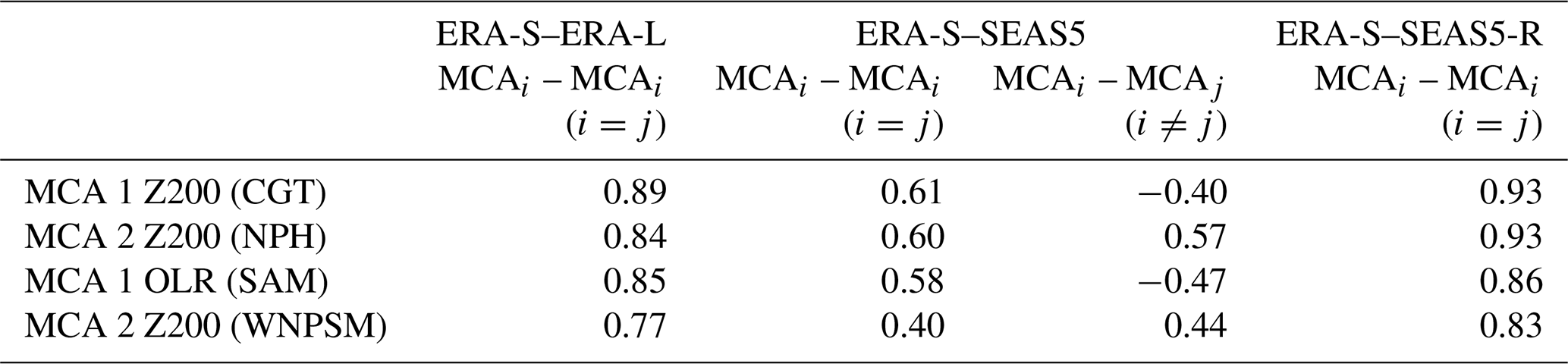
Table 2 Spatial pattern correlation between MCA modes obtained from ERA5 data over the periods 1979–2020 and 1993–2016, between ERA5 and SEAS5 data over the common period 1993–2016 and for the same period but as the projection of ERA5 MCA (see main text for more details). All numbers are significant at α=0.05.

2.3 PCMCI and causal maps

The PCMCI algorithm is a causal discovery method using conditional statistical association strengths to iteratively test for causality between two (or more) time series (actors) given a certain set of conditioning variables (Runge, 2018; Runge et al., 2014, 2019; Spirtes et al., 2000). The term causal builds upon a series of hypotheses, such as causal sufficiency (i.e. all relevant actors are included in the analysis) and stationarity of the detected causal chain (i.e. the causal links are stationary over time and actors show no trend). Hence, the detected causal links are valid in the set of analysed actors and also depend on the linear or non-linear framework applied (here, we employ linear partial correlations since they can be estimated in a more robust way from time series of limited length than their nonlinear counterparts and allow defining the direction of an effect relative to the cause) as well as a set of parameters, such as the significance threshold α. The causal links identified by PCMCI are represented in a so-called causal effect network (CEN), a graph where each actor is represented by a node and causal links are shown as arrows connecting different nodes (Fig. 2a). The sign and strength of a certain causal link are given by the β coefficient, represented in the CEN by the colour of an arrow. For example, given the causal link actor2${}_{\mathit{\tau }=-\mathrm{1}}\to$ actor1_τ=0, a β coefficient of 0.25 represents a positive change of 0.25 standard deviation (SD) of actor1 at lag 0 due to a positive change of 1 SD in actor2 at lag −1.

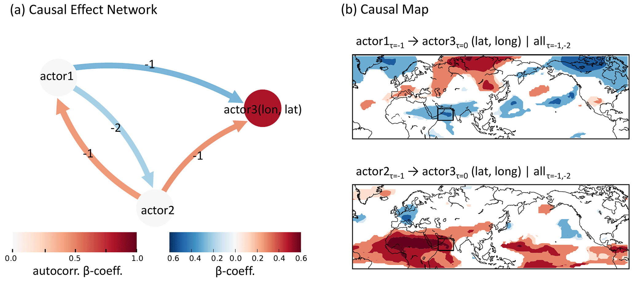
Figure 2 Schematic representation of CEN and causal map. Panel (a) shows an example of a CEN built with three actors and lag_max −2. Panel (b) shows an example of a causal map: the β value for the causal effect of actor1 and actor2 on actor3 (a time-varying field) varies with the latitude and longitude in the map.

Here we apply the concept of causal maps, an extension of PCMCI to spatial fields of variables, to analyse the influence of a set of spatial patterns representing tropical–extratropical summer interactions (identified by applying MCA) on a 2D field (Di Capua et al., 2020a). Causal maps make use of the concept of CEN and the PCMCI algorithm. However, instead of showing the typical network-like shape with actors connected by arrows representing the direction, sign and strength of the causal links as shown in Fig. 2a, causal maps provide information in a similar conceptual manner to a classical correlation map (Fig. 2b). In a causal map, however, each grid point represents the sign and strength (given by the β coefficient) of a certain causal link, e.g. between actor1 and actor3, while the direction of the link and the set of actors involved is kept constant throughout each map (more maps are necessary to show different configurations of actors as shown in Fig. 2b).

To provide a meaningful comparison with previous work, in this analysis we apply the same framework as used in Di Capua et al. (2020a); i.e. each causal map is obtained by running at grid point level a CEN analysis with three actors. Of these three actors, two represent the pair of time series obtained for each MCA mode and are kept constant throughout the map (actor1 and actor2 in our example in Fig. 2a). The third time series is the time series for any individual grid point of the considered time-varying field (OLR or Z200) and thereby depends on longitude and latitude (actor3(lat, lon) in Fig. 2a). Thus, for each MCA mode we will have eight causal maps, as we have two target fields (OLR and Z200), two MCA modes and two MCA time series for each MCA mode (one for tropical OLR and one for mid-latitudes Z200). This can be summarised in Eq. (1):

$$\begin{array}{}\text{(1)}& {\mathrm{MCA}}_i^k\to {\mathrm{field}}_j\mathrm{|}{\mathrm{MCA}}_{i\ne l}^k,\end{array}$$

where $i,l\in \mathit{\{}\mathrm{trop}.\mathrm{OLR},\mathrm{midlat}.\mathrm{Z}\mathrm{200}\mathit{\}}$, $j\in \left\{\mathrm{Z}\mathrm{200},\mathrm{OLR}\right\}$ and $k\in \left\{\mathrm{1},\mathrm{2}\right\}$ are the two MCA modes. Note that when conditioning on ${\mathrm{MCA}}_{i\ne l}^k$, i needs to be different from l since when testing the influence of actor1 on actor3(lat, lon) we want to remove the influence of actor2. Thus, if ${\mathrm{MCA}}_i^k={\mathrm{MCA}}_{\mathrm{trop}.\mathrm{OLR}}^{\mathrm{1}}$, then ${\mathrm{MCA}}_l^k={\mathrm{MCA}}_{\mathrm{midlat}.\mathrm{Z}\mathrm{200}}^{\mathrm{1}}$.

Here, we use PCMCI version 4.1 from the Python package tigramite (https://github.com/jakobrunge/tigramite, last access: 2 August 2023). We estimate causal maps with the parameters lag${}_{\min }=-\mathrm{1}$, lag${}_{\max }=-\mathrm{2}$ (units of the sampling period, i.e. weeks) and pc_alpha = 0.2 (unless otherwise indicated we use the default parameters of PCMCI). Note that only results for lag −1 are shown as almost no significant links are found for lag −2 in ERA5 causal maps. Note that pc_alpha is not the final significance threshold adopted to determine the significance of the identified causal links; instead it is a parameter used in the PC step of the PCMCI algorithm, which if taken too strictly (e.g. the usual α= 0.05) would prevent the algorithm from retaining some potentially meaningful links (for further details see https://jakobrunge.github.io/tigramite/, last access: 2 August 2023).

The significance threshold adopted for plotting the results is α= 0.05 (for a time series length of 600 years) and 0.1 (for a time series length of 24 years), and we use corrected p values by applying a false-discovery rate (FDR) correction (Benjamini and Hochberg, 1995) to control for multiple testing among the multiple grid locations in causal maps. The false-discovery rate is “the expected proportion of erroneous rejections among all rejections” (Benjamini and Yekutieli, 2001).

2.4 Subsampling experiments

We perform two subsampling experiments: Experiment A aims to better understand differences in the strength of causal links between ERA-S and SEAS5-R, while Experiment B evaluates the spread inside the SEAS5 ensemble. For each subsampling experiment, we select 1000 samples of 24 years each (for each year, one ensemble member is randomly selected out of the 25 available members), and for each sample we provide the corresponding causal map. In this way, the number of years used in each subsampling experiment (24 years) is the same as those available from ERA-S (24 years). Reducing the length of the time series in this way increases the variability and hence lowers the significance of the obtained β values. However, this should not by itself lower the strength of the β values themselves. Thus, a priori, we might expect fewer regions to show a significant β value in a smaller dataset than in a larger one but not a difference in the strength of the β values. Hence, this 1000-ensemble member subsampling experiment allows us to evaluate the distribution of β values around their mean value and to compare it to the ERA-S values of reference. For each causal map, the p values are corrected by applying the Benjamini–Hochberg false-discovery rate correction, and only β values with a corrected p value < 0.1 are retained.

In Experiment A, we impose the set of causal parents which have been detected as significant for ERA5 in the SEAS5 ensemble and then calculate the corresponding causal effect in SEAS5. In this way, we provide a fairer comparison between the strengths of β_ERA5 and β_SEAS5. In other words, SEAS5-R causal maps obtained from Experiment A will show significant causal links for the same grid points as in ERA5 causal maps, but the sign and the strength of the β coefficient will vary following the physical representation of these teleconnections in the SEAS5 dataset. However, we cannot a priori assume that all the causal links detected in ERA5 will be reproduced by the SEAS5 forecast with the same sign, direction and strength (which would be the equivalent of assuming that the effect of sampling variability in ERA5 on the selection of causal links is zero and that the model does a perfect job in reproducing all observed teleconnections, while instead well-known biases between the model and the reanalysis products are observed; e.g. Johnson et al., 2019). Therefore, in Experiment B we let the PCMCI algorithm identify the causal parents in SEAS5 and then estimate the causal effect. Thus, new causal links that were not detected in ERA5 may appear, while others that were significant in the reanalysis dataset may disappear. Analysing the results for these two subsampling experiments will enable us to compare the strength, sign and location of tropical–extratropical teleconnections between SEAS5 and ERA5.

3 Results

This section is organised as follows: first we define and describe MCA patterns both in ERA5 and SEAS5 datasets (Sect. 3.1). Then we calculate the respective causal maps and compare those obtained in ERA5 with those obtained with SEAS5 (Sect. 3.2). In Sect. 3.3 we produce a 1000-member subsampling experiment by imposing the causal parents found in ERA5-S to determine whether ERA5 β values fall in the range of realisations of SEAS5 (Experiment A). In Sect. 3.4 we use the same subsamples but allow the PCMCI algorithm to freely detect causal links in SEAS5 (Experiment B). Following those studies, in Sect. 3.5, we check whether ENSO may influence these tropical–extratropical teleconnections and what role model biases may play in explaining ERA5–SEAS5 differences.

3.1 MCA patterns in SEAS5 and ERA5

We first derive the two leading maximum covariance analysis (MCA) coupled modes of tropical–extratropical co-variability between mid-latitude (25–75^∘ N) geopotential height at 200 hPa and tropical (15^∘ S–30^∘ N) outgoing long-wave radiation in ERA5 reanalysis data for the period 1993–2016 (ERA-S; Fig. 3). MCA modes found for the extended period 1979–2020 (ERA-L) are shown in Fig. S1 in the Supplement. The two pairs of patterns identified in this way are the South Asian monsoon (SAM; Fig. 3d) paired with the circumglobal teleconnection (CGT; Fig. 3a) pattern for MCA mode 1 and the western North Pacific summer monsoon (WNPSM; Fig. 3j) paired with the North Pacific high (NPH; Fig. 3g) for MCA mode 2.

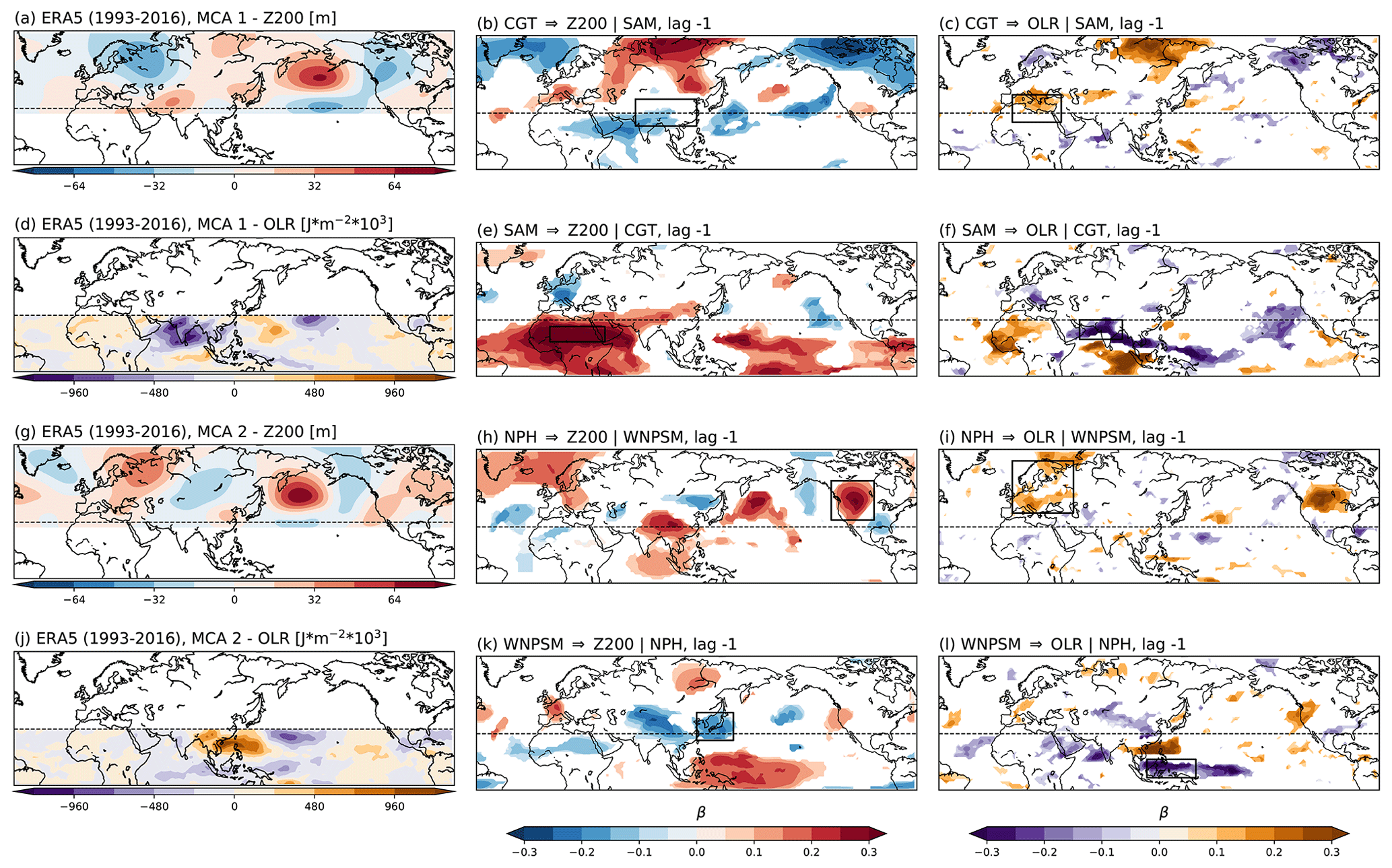
Figure 3 Causal maps for ERA5. Left column: MCA patterns for Z200 and OLR fields for ERA-S. MCA mode-1 Z200 (a) shows the CGT pattern. MCA mode-1 OLR shows the SAM (d). MCA mode-2 Z200 shows the NPH (g). MCA mode-2 OLR shows the WNPSM (j). Central column (b, e, h, k) shows causal maps for the effect of each MCA pattern on Z200 fields. Right column (c, f, i, l) shows causal maps for the effect of each MCA pattern on OLR fields. The black boxes highlight Southeast Asia (b), the Mediterranean (c), the Sahel region (e) and India (f) for MCA mode 1 and central western USA (h), eastern Europe (i), Japan (k) and the Maritime Continent (l) for MCA mode 2. Refer to the text in Sect. 3.2 for an interpretation of the results. Only grid points with corrected p values significant at α= 0.1 are shown.

The SAM is characterised by a large rainfall band stretching from the Arabian Sea towards the western edge of the South China Sea, with a peak of negative OLR (relatively high rainfall) centred over the Indian peninsula (Fig. 3d). The CGT pattern shows five centres of positive Z200 anomalies over the Iberian Peninsula, central Asia on the eastern side of the Caspian Sea, eastern China, the North Pacific and the southeastern USA (Fig. 3a). The WNPSM pattern features a region of enhanced convective activity over the tropical western Pacific between 25 and 30^∘ N accompanied by an area of suppressed convective activity on its western side centred over the South China Sea (Fig. 3j). The main feature of the NPH is a ridge in Z200 located at the western side of the North Pacific; however this pattern also shows a zonally oriented wave train like the CGT pattern but with centres of action shifted in longitude (Fig. 3g). These four patterns can explain up to 25 % of the variance in the Z200 and OLR fields depending on the region (not shown).

The key features described above for the ERA-S MCA modes 1 and 2 (Fig. 3a, d, g, j) are qualitatively very close to those found for the 1979–2020 period (ERA-L; Fig. S1a, d, g, j) or ERA-Interim (Figs. 3 and 4 in Di Capua et al. 2020a). The spatial correlation between ERA-L and ERA-S MCA modes ranges between 0.8 and 0.9 (Table 2), showing that these patterns are robust across different versions of ERA reanalysis and quite insensitive to the chosen period. However, when MCA modes are calculated on SEAS5 seasonal forecasts initialised on the 1 May and compared to ERA-S, a few key differences arise (Fig. S2). Overall each ERA-S MCA mode (Fig. 3a, d, g, j) shares common features with its corresponding SEAS5 MCA mode (Fig. S2a, d, g, j). This similarity can be quantified by calculating the spatial correlation of each ERA-S MCA mode shown in Fig. 3a, d, g and j with the corresponding SEAS5 MCA mode in Fig. S2a, d, g, and j, for both the tropical belt (15^∘ S–30^∘ N, 0–360^∘ E) and the mid-latitude region (25–75^∘ N, 0–360^∘ E). Results are shown in Table 2 (second column) and yield values ranging between 0.4 and 0.6.

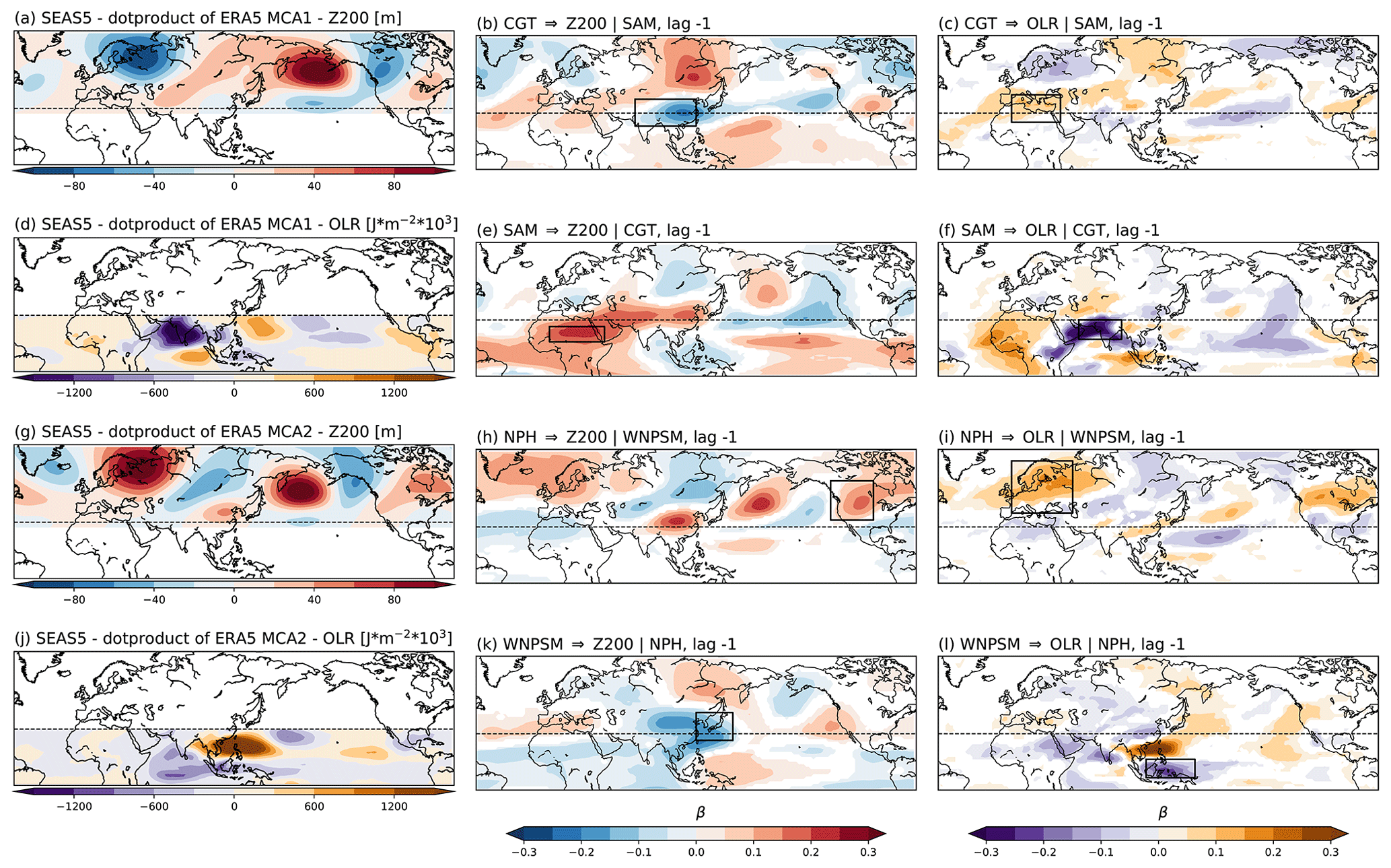
Figure 4 Causal maps for SEAS5-R. SEAS5-R MCA (calculated as the projection of ERA-S on SEAS5 Z200 and OLR fields) and related causal maps. Left column: MCA patterns for Z200 and OLR fields for SEAS5-R calculated as composites of time steps with the MCA time series values higher than 1 standard deviation (SD). MCA mode-1 Z200 (a) shows the CGT pattern. MCA mode-1 OLR shows the SAM (d). MCA mode-2 Z200 shows the NPH (g). MCA mode-2 OLR shows the WNPSM (j). Central column (b, e, h, k) shows causal maps for the effect of each MCA pattern on Z200 fields. Right column (c, f, i, l) shows causal maps for the effect of each MCA pattern on OLR fields. The black boxes highlight Southeast Asia (b), the Mediterranean (c), the Sahel region (e) and India (f) for MCA mode 1 and central western USA (h), eastern Europe (i), Japan (k) and the Maritime Continent (l) for MCA mode 2. Refer to the text in Sect. 3.2 for an interpretation of the results. Only grid points with corrected p values significant at α= 0.05 are shown (see “Data and methods” for further details).

However, some features that in ERA-S characterise MCA 1 are also found in SEAS5 MCA 2 and vice versa for ERA-S MCA 2. Thus, features that in ERA-S are separated and characterise each of the first two MCA modes appear mixed in SEAS5 (or vice versa). For example, in ERA-S the CGT-related high to the east of the Caspian Sea is only visible in MCA 1 (Fig. 3a), while in SEAS5, the same positive signal is found in both MCA 1 and MCA 2 (although stronger in MCA 1). Similarly, the convective activity over the Indian peninsula, which in ERA-S represents one of the characteristic features of MCA 1 (Fig. 3d) and is very weak in MCA 2 (Fig. 3j), is found in both MCA 1 and MCA 2 of SEAS5 almost with similar magnitudes, though the negative anomalies are stronger in MCA 1 (Fig. S2d, j). In contrast, the wave pattern over Eurasia characterising ERA-S MCA 2 showing a high-pressure region over eastern Europe and a low over central Asia (Fig. 3g) is very weak in SEAS5 MCA modes 2 (Fig. S2g) and not present in MCA mode 1 (Fig. S2a). This can be seen in spatial correlation values calculated between ERA-S MCA 1 (MCA 2) and SEAS5 MCA 2 (MCA 1) which also range between 0.4 and 0.6, although sometimes with reversed sign (opposite phase of the pattern) (Table 2, third column). Therefore, we conclude that despite the general resemblance of the first two SEAS5 MCA modes to those calculated in ERA-S, working with a mixed signal would hinder the interpretability of parts of the results, since it would make it difficult to effectively separate the causal effect of the SAM–CGT patterns from that of the WNPSM–NPH pair.

To account for this problem, SEAS5 MCA modes have been re-calculated by projecting ERA-S MCA patterns onto SEAS5 Z200 and OLR 3D fields, as explained in Sect. 2.2. Then, to visualise the equivalent SEAS5-R MCA modes (where SEAS5-R depicts the MCA modes calculated by projecting ERA-S MCA patterns onto SEAS5 fields), composites of time steps with the MCA time series values higher than 1 standard deviation (SD) are calculated (Fig. 4a, d, g, j). As a result, a much closer resemblance between SEAS5-R and ERA-S MCA patterns is obtained and the spatial correlation coefficients between SEAS5-R and ERA-S MCA patterns reach values of ∼0.8–0.9 (Table 2, fourth column). Note that the difference in the magnitude of the anomalies shown in Figs. 3a, d, g, and j and Figs. 4a, d, g and j is greatly diminished if ERA5 MCA patterns are plotted with the same methods, i.e. plotting composites of time steps with the MCA time series values higher than 1 SD (see Figs. S3 and S4 in the Supplement). In the remainder of this paper, we will analyse the causal effect of the SEAS5-R MCA modes shown in Fig. 4.

3.2 Causal maps in SEAS5 and ERA5

Having defined ERA-S and SEAS5-R MCA modes, we apply the concept of causal maps to detect the causal effect of each of these four patterns (two for each mode) on Z200 and OLR fields, in the range 15^∘ S–75^∘ N.

Causal maps calculated for the effect of ERA-S CGT and SAM at lag −1 on Z200 and OLR fields are shown in Fig. 3b–c and Fig. 3e–f respectively. Note that both the CGT–SAM time series pair and the NPH–WNPSM pair share a significant correlation of r∼0.5–0.6 at lag 0 (Table S1 in the Supplement). In contrast, the SAM–WNPSM and CGT–NPH pairs show a non-significant correlation close to r∼0. Thus, we analyse the two MCA pairs separately. The main features are the effect of SAM on Sahel Z200, the tropical Pacific Ocean, a high–low pattern in the North Pacific and the negative effect on Z200 in central Europe (Fig. 3e). A positive causal effect (positive β value) of SAM on Sahel Z200 means that enhanced rainfall over the Indian monsoon region tends to be followed 1 week later by higher Z200 anomalies over the Sahel region and the tropical Pacific. In contrast, increased SAM activity leads to negative β values over central Europe Z200, positive β values southwest of Alaska and negative β values in the eastern North Pacific Z200 (Fig. 3e). A positive causal effect (positive β values) of the CGT pattern on Z200 is mostly concentrated in the subtropical North Atlantic; southern Europe; central, northern and eastern Asia; the North Pacific; and southeastern USA (Fig. 3b). Thus, these regions will experience positive Z200 anomalies 1 week after an enhanced CGT pattern. In contrast, the North Atlantic (around Iceland), southern Asia and the Arabian Sea, the eastern North Pacific, the Philippine Sea, and Canada will experience negative Z200 anomalies (negative β values; Fig. 3b). In general, β values for OLR causal maps (Fig. 3c and f) mirror those for the Z200 field in the mid-latitudes, while in the tropics they add the information on tropical convective activity, which is not detected by Z200 anomalies. In Fig. 3c negative β values over southern India indicate that an enhanced CGT pattern leads to lower OLR values and thus increased convective activity over the region. In Fig. 3f the tilted band of convective activity stretches from the Arabian Sea and central India towards the Maritime Continent. This convective activity is related to the boreal summer intraseasonal oscillation (BSISO), as shown in Di Capua et al. (2020a).

Causal maps calculated for the effect of NPH and WNPSM on Z200 and OLR fields are shown in Fig. 3h and i and Fig. 3k and l, respectively. Causal maps for the effect of NPH on Z200 and OLR fields display a zonally oriented pattern that encircles the northern mid-latitudes (Fig. 3h, i). Positive β values in Fig. 3h indicate that an enhanced NPH pattern (Fig. 3g) leads to positive Z200 anomalies over the North Atlantic (around Iceland), southeastern China, the NPH region and the northwestern USA. Negative β values over central and eastern Asia and over the eastern North Atlantic indicate that an enhanced NPH pattern is followed 1 week later by negative Z200 anomalies over these regions. The effect of WNPSM is more confined to eastern Asia and the North Pacific, where an arch-shaped pattern stretches from the tropical western Pacific, reaching Alaska and the US west coast (Figs. 3k, l and S1k, l). Suppressed convective activity over the South China Sea and the Philippine Sea and increased convective activity over the WNPSM are followed 1 week later by negative Z200 anomalies over Southeast Asia and central Asia and positive Z200 anomalies over northeastern Asia and the US west coast (Fig. 3k, l).

In general, a two-way causal link between tropical convection and mid-latitude circulation is shown for both MCA modes: the causal effect of SAM and WNPSM reaches the northern mid-latitudes, while the effect of the mid-latitude CGT pattern and NPH extends to subtropical latitudes. Consistent results are obtained for ERA-L (see Fig. S1) with more significant causal links (likely due to the increased length of the 1979–2020 time series), improving the clarity of the spatial patterns. These patterns also show great resemblance to those produced using the ERA-Interim reanalysis in Di Capua et al. (2020a) (see their Figs. 3 and 4).

Causal maps produced with SEAS5-R MCA modes and SEAS5 OLR and Z200 fields using all the available 600 years (Fig. 4) show similar spatial patterns to those obtained with ERA-S (Fig. 3). In general, the sign and the geographical position of the causal links detected in SEAS5 are consistent with those found in ERA5, meaning that the effect of each MCA mode on the analysed fields is consistent in sign and spatial location between the two datasets. For example, the link SAM${}_{\mathit{\tau }=-\mathrm{1}}\to$ Z200_τ=0 |CGT${}_{\mathit{\tau }=-\mathrm{1}}$ shows a positive causal effect on the Sahel region both in ERA5 and SEAS5 (Figs. 3e and 4e). Thus, the first key result obtained in this section is that the main tropical–extratropical intraseasonal causal relationships in boreal summer in the Northern Hemisphere are at least qualitatively well represented in the SEAS5 system. These causal maps also show that the two-way causal pathway between tropical convective activity and extratropical circulation is captured by the seasonal forecasts. Thus, on the one hand we gain confidence in the interpretation of the earlier ERA-Interim and ERA-S/L causal map analysis, which is reproduced by SEAS5, and on the other hand we show that, to a first approximation, seasonal forecasts can reproduce such causal links.

When SEAS5 MCA modes, which capture the strongest co-variability signal in SEAS5 seasonal forecasts, are used to produce causal maps (see Supplement, Fig. S2), similar spatial structures and signs of the causal links are detected. To compare the strength of the β coefficients in ERA5 and SEAS5, we proceed by using the subsampling technique as described in Sect. 2.4. Note that comparing β coefficients obtained using a time series of 600 years (SEAS5-R) with those calculated using 24 years (ERA5-S) would not represent a good way to assess differences in the strength of the causal signal.

3.3 Causal effect strength in SEAS5 and ERA5

To assess the difference in strength between SEAS5-R and ERA-S β values, we use the causal maps obtained from subsampling Experiment A, as described in Sect. 2.4. To make sure that we properly assess changes in the strength of the causal effect between the two datasets, we (a) use the same number of years as in ERA5-S (24 years) and (b) fix the direction and significance of the causal links for each grid point to be the same as those detected for the ERA5 dataset (Fig. 3). As an example, if we analyse the effect of SAM and CGT on the Z200 field in the ERA5 dataset for the grid point at 20^∘ N, 16^∘ E, we find a significant positive β coefficient for the link SAM → Z200|CGT and a significant negative β for the link CGT → Z200|SAM (plus a certain self-influence of the Z200 time series on itself). Then, we calculate the corresponding β coefficients for each of the 1000 SEAS5 subsamples by imposing the same causal parents as those found in ERA5. This way, we obtain a set of 1000 β coefficients, for each analysed causal link and for each grid point, which would be visualised in 1000 causal maps (see Fig. S6a). The causal maps obtained by averaging these 1000 causal maps are shown in Fig. 5a, d, g and j for links CGT → Z200|SAM, SAM → Z200|CGT, CGT → OLR|SAM and SAM → OLR|CGT, respectively. In general, the strengths of the β values obtained in Fig. 4 tend to be of the same magnitude as the mean β values obtained in the 1000 subsamples.

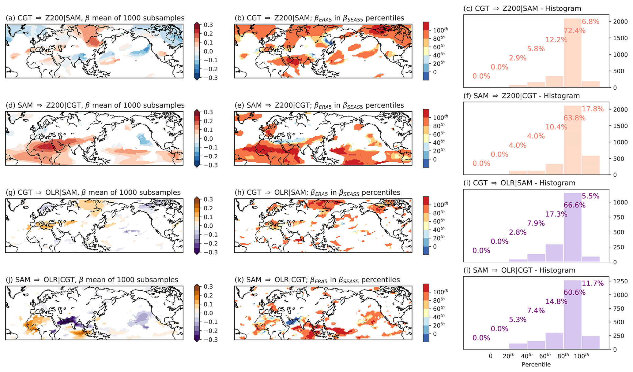
Figure 5 Strength of the β coefficients in subsampling Experiment A for MCA 1. (a) Causal effect for CGT → Z200|SAM averaged over the 1000 subsamples obtained in the SEAS5 dataset (initialised on 1 May). Direction and significance of the causal links are imposed to be the same as calculated in Fig. 3. (b) β_ERA5 compared to β_SEAS5 quantiles for the CGT → Z200|SAM link. (c) Histogram showing the percentage of grid points for which the β_ERA5 falls in a certain quantile range as obtained for β_SEAS5 coefficients. Panels (d), (e) and (f) are the same as for panels (a), (b) and (c) but for the SAM → Z200|CGT link. Panels (g), (h) and (i) are the same as for panels (a), (b) and (c) but for the CGT → OLR|SAM link. Panels (j), (k) and (l)  are the same as for panels (a), (b) and (c) but for the SAM → OLR|CGT link.

Next, we compare the β_ERA5 absolute values to the absolute values of the 1000 β_SEAS5 obtained in subsampling Experiment A. Here we use absolute values as we intend to compare the strength of the β coefficients and not the sign. Notably, the average percentage of β values in the subsampling experiment for which the sign does not agree with that of β_ERA5 is ∼20 %. Note that fixing the set of causal parents implies that the β coefficients are calculated by regressing on the same set of parents used for ERA-S; however in SEAS5 the sign and strength of the β coefficient can still vary. For each grid point, we calculate the probability density function describing the distribution of the 1000 β_SEAS5 and estimate the 0th, 20th, 40th, 60th, 80th and 100th percentiles (Fig. S6b). Then, we categorise the β_ERA5 as falling into one of the selected quantile ranges or above/below the maximum/minimum of the distribution. For example, in Fig. S6 the β coefficients for the grid point at 20^∘ N, 16^∘ E are analysed, and the β_ERA5 value is shown to fall beyond the 100th percentile, meaning that for that grid point, all of the 1000 β_SEAS5 coefficients are smaller in strength than the observed β_ERA5 value. The overall results for the analysed region are shown in Fig. 5b, e, h and k, where yellow shaded grid points indicate that β_ERA5 coefficients fall in the middle of the β_SEAS5 distribution, while blue/red shaded grid points indicate β_ERA5 coefficients falling in the lowest/uppermost tails of the β_SEAS5 distribution.

In general, for MCA 1 orange/red colours dominate all four causal maps, among which tropical and high-latitude regions show the most underestimated β_SEAS5 values compared to the β_ERA5 reference point (Fig. 5b, e, h, k). Histograms describing the percentage of grid points falling in each category for each causal map are shown in Fig. 5c, f, i and l. Results show that β_ERA5 values for the vast majority (∼70 %) of the grid points fall above the 80th β_SEAS5 percentile, and about 5 %–20 % fall above the 100th percentile, meaning that the SEAS5 subsamples are never able to reproduce the observed β_ERA5 values for those specific grid points. In contrast, the few regions where the strength of β_SEAS5 is overestimated include the Middle East and the Arabian Sea. Similar results are shown for MCA 2 (Fig. 6), with β_ERA5 values exceeding the 80th percentile of the SEAS5 subsample distribution for 60 %–70 % of the grid points. The percentage of grid points exceeding the 100th percentile is however reduced compared to MCA 1, with only 1 %–10 % of the grid points showing β_ERA5 values exceeding the maximum β_SEAS5 of the distribution.

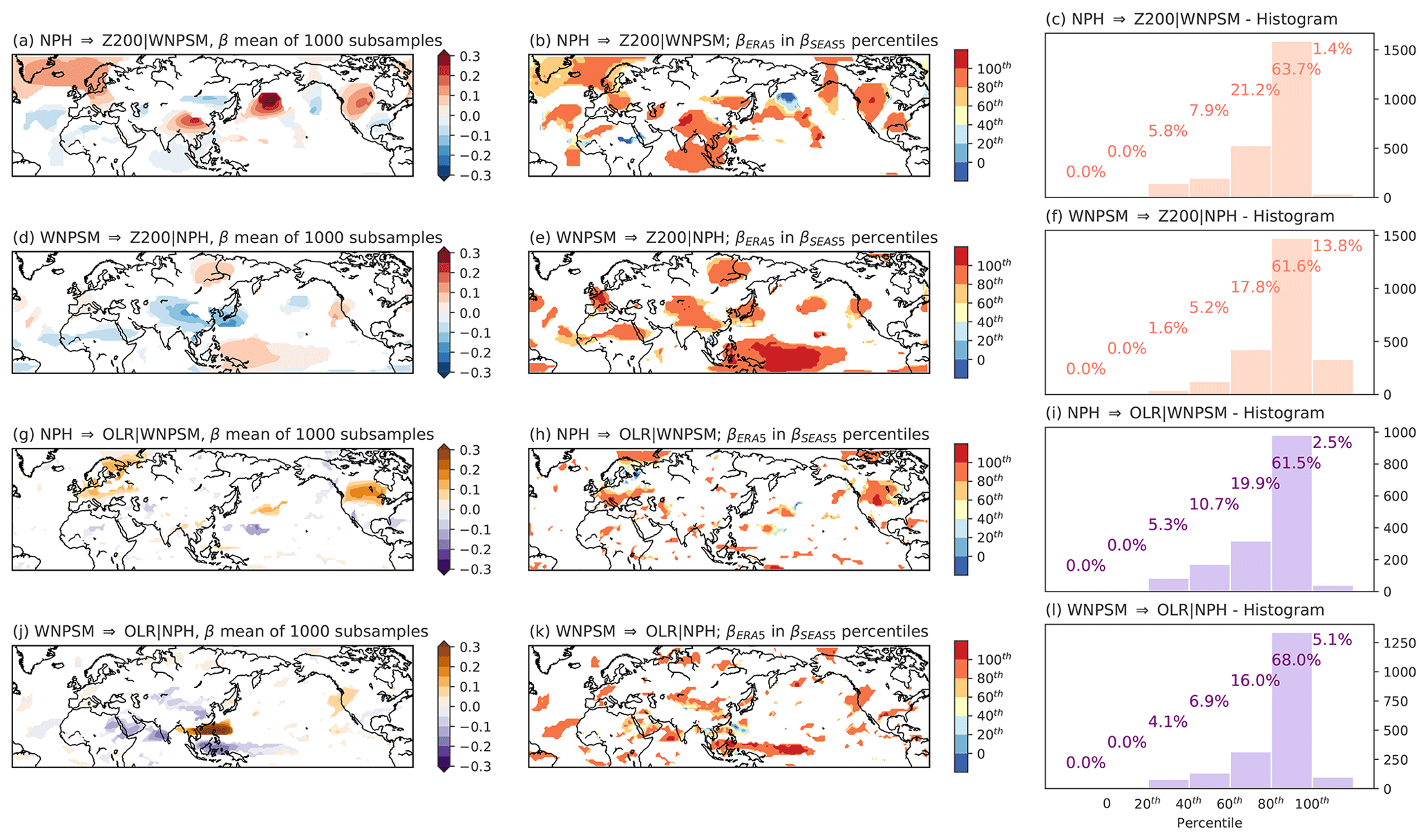
Figure 6 Strength of the β coefficients in subsampling Experiment A for MCA 2.  (a) Causal effect for NPH → Z200|WNPSM averaged over the 1000 subsamples obtained in the SEAS5 dataset (initialised on 1 May). Direction and significance of the causal links are imposed to be the same as calculated in Fig. 3. (b) β_ERA5 compared to β_SEAS5 quantiles for the NPH → Z200|WNPSM link.  (c) Histogram showing the percentage of grid points for which the β_ERA5 falls in a certain quantile range as obtained for β_SEAS5 coefficients. Panels (d), (e) and (f) are the same as for panels (a), (b) and (c) but for the WNPSM → Z200|NPH link. Panels (g), (h) and (i) are the same as for panels (a), (b) and (c) but for the NPH → OLR|WNPSM link. Panels (j), (k) and (l) are the same as for panels (a), (b) and (c) but for the WNPSM → OLR|NPH link.

The dependence of causal maps on the time of initialisation of SEAS5 has also been analysed. The same plots as Figs. 4–6 produced with SEAS5 seasonal forecasts initialised on 1 March (rather than 1 May) are shown in the Supplement (see Figs. S5, S7–S8). Figures 4–6 are very consistent with Figs. S5, S7 and S8; thus the initialisation date of SEAS5 does not have a qualitative influence on the causal maps calculated over the entire 1993–2016 period. The apparent independence of the initialisation date is most likely explained by the independence of the β coefficients of the absolute values of a certain variable in a specific year. As explained in Sect. 2, the β coefficients represent the relative change in SD of one actor given a certain change in the values of its parents (expressed in SD).

Finally, in Fig. 7 we check that the observed tendency towards underestimation of causal effect strengths does not depend on the chosen p-value threshold (also see the Supplement, Sect. S1 and Fig. S9). We demonstrate that even using non-causal β values, i.e. those β values calculated for grid points where the p value > 0.1 and therefore not representing causal links in Figs. 3, 5 and 6, the underestimation by SEAS5, though less strong, still dominates all causal maps (Fig. 7). We would like to highlight that, using a p value = 1.0 (i.e. no threshold), up to 80 % of the obtained β values do not represent causal links. Nevertheless, a peak between the 80th and 100th percentiles is still clearly also visible for very high p values, and the number of β values that fall above the 80th percentile (which should be 20 % in case an underestimation effect of the β_ERA5 is not present) is still found between 30 % and 49 % even in the most extreme case (p value = 1.0). Thus, we can confidently state that, qualitatively, the underestimation of β_ERA5 by SEAS5 does not depend on the chosen p value. However, the exact magnitude of the underestimation effect, i.e. the obtained β values for each p-value threshold, can vary.

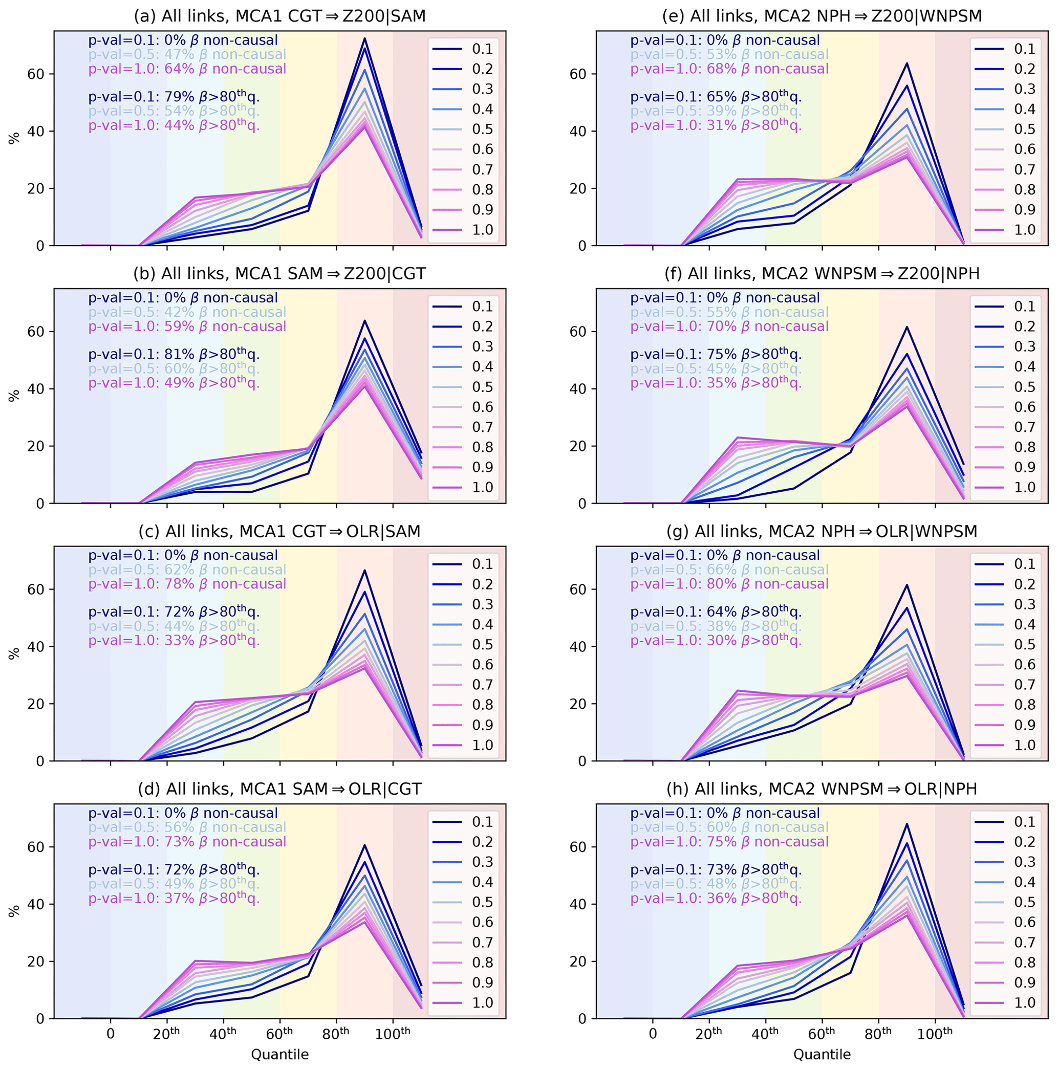
Figure 7 Experiment A, sensitivity test. (a) Histogram showing the percentage of grid points for which β_ERA5 falls in a certain quantile range as obtained for β_SEAS5 coefficients for the link CGT → Z200|SAM. Panel (b) is the same as for panel (a) but for the link SAM → Z200|CGT. Panel (c) is the same as for panel (a) but for the link CGT → OLR|SAM. Panel (d) is the same as for panel (a) but for the link SAM → OLR|CGT. Panel (e) is the same as for panel (a) but for the link NPH → Z200|WNPSM. Panel (f) is the same as for panel (a) but for the link WNPSM → Z200|NPH. Panel (g) is the same as for panel (a) but for the link NPH → OLR|WNPSM. Panel (h) is the same as for panel (a) but for the link WNPSM → OLR|NPH. In each panel, the percentage of non-causal grid points analysed and the percentage of grid points for which the β values exceeds the 80th percentile is highlighted for p values in the range {0.1, 0.5, 1.0}.

3.4 Causal effect spread in the SEAS5 ensemble

To assess whether the location, sign and strength of the causal links change between SEAS5 and ERA5 when the PCMCI algorithm is run in the 1000 subsamples of SEAS5 without imposing ERA5 causal parents, the results from subsampling Experiment B are analysed (see Sect. 2.4). The resulting 1000 causal maps are averaged and shown in the left column in Figs. 8 and 9. For each grid point, the mean β value is calculated only if at least 100 β value results are significant at an α= 0.10 level; however, non-significant values are not allowed to enter the mean. Applying this double threshold (which is not done in Fig. 3) notably shrinks the area of spatial patterns compared to those in Figs. 3 and 4; however here we concentrate only on the β values contained in the regions highlighted by black boxes in Figs. 8 and 9.

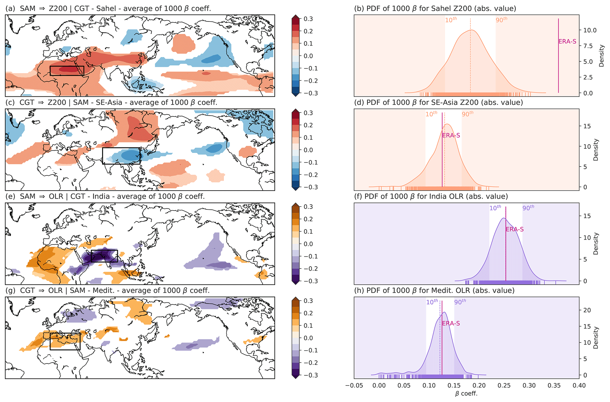
Figure 8 Ensemble spread for subsampling Experiment B for MCA mode 1. The mean causal effect is averaged over four key regions. Mean causal effect averaged over the 1000 subsamples for SAM → Z200|CGT (a), CGT → Z200|SAM (c), SAM → OLR|CGT (e) and CGT → OLR|SAM (g). Only grid point with β coefficients significant at α= 0.10 (after applying the Benjamini–Hochberg false-discovery rate correction) are shown. PDFs for the absolute values of the 1000 β coefficients are shown with highlighted 10th and 90th percentiles for the Sahel region (b), Southeast Asia (d), India (f) and the Mediterranean (h). β coefficients for ERA-S are shown in the PDFs for comparison by a vertical solid magenta line. The black boxes highlight the Sahel region (a), Southeast Asia (c), India (e) and the Mediterranean (g). The significance of the β coefficients shown in the causal maps in panels (a), (c), (e) and (g) is described in Sect. 3.4.

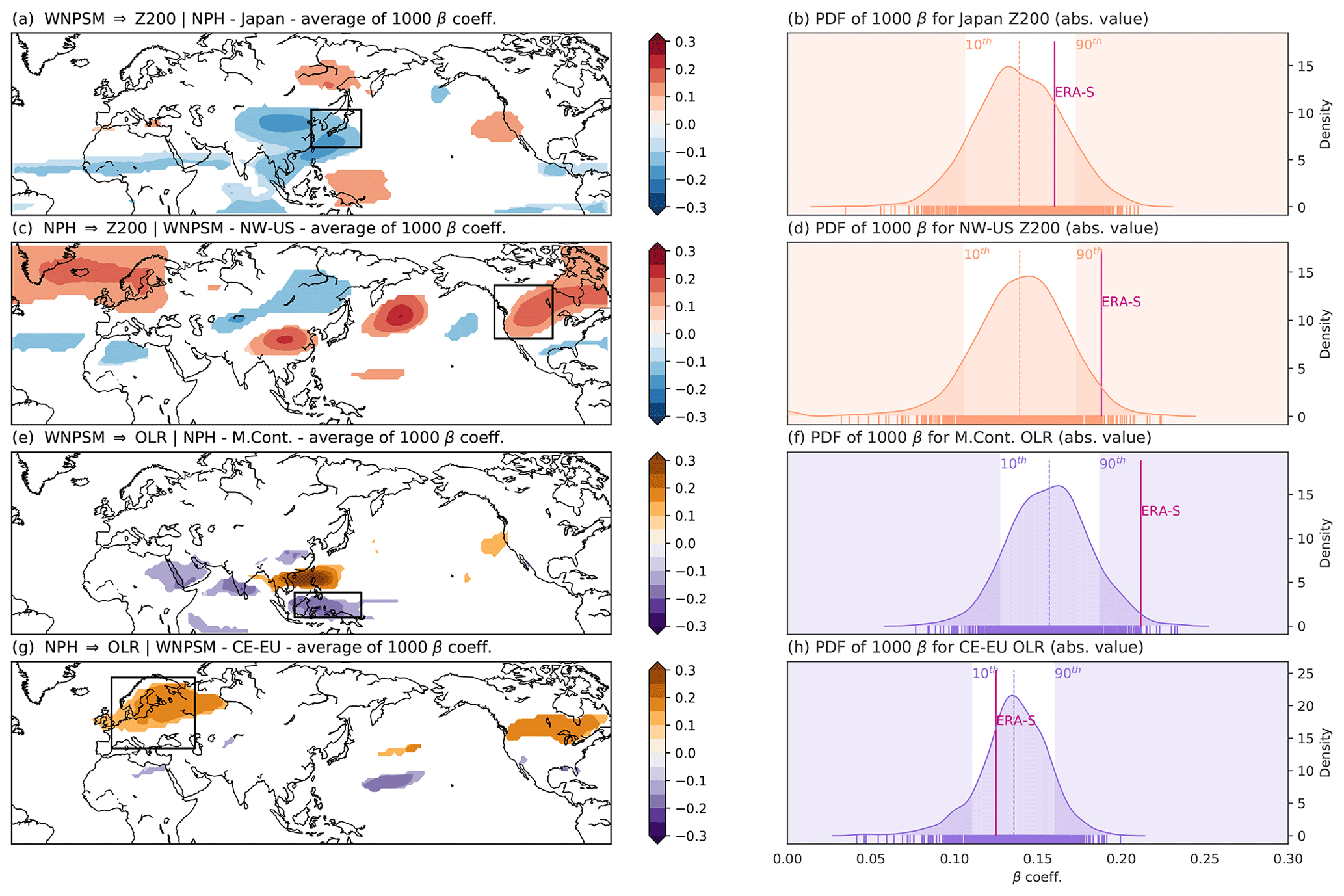
Figure 9 Ensemble spread for subsampling Experiment B for MCA mode 2. Same as for Fig. 8 but for MCA mode 2. Mean causal effect averaged over the 1000 subsamples for WNPSM → Z200|NPH (a), NPH → Z200|WNPSM (c), WNPSM → OLR|NPH (e) and NPH → OLR|WNPSM (g). PDFs for the absolute values of the 1000 β coefficients are shown for Japan (b), northwestern USA (d), Maritime Continent (f) and central eastern Europe (h).

Due to the complexity of the spatial patterns shown in the causal maps in Fig. 3, and to the smaller number of significant grid points available in ERA-S compared to SEAS5-R (as visualised in Figs. 3 and 4), calculating spatial correlations is not the most appropriate way to compare the two sets of causal maps. A high (or low) spatial correlation may result from strong or weak agreement in different regions, but it would not be possible to discern from which specific area the signal is originating. Moreover, the position of the significant links is not the same between ERA-S and SEAS5 subsampling Experiment B.

To provide a meaningful comparison, we choose four key regions for each MCA mode, and for those regions we analyse the characteristics of the causal effect in detail. We identify these regions based on (i)  the prominence of the signal in Figs. 3 and 4 and/or (ii) the misrepresentation of the strength of the β values in Figs. 5 and 6. By applying these criteria, the chosen geographical regions (shown in Figs. 8 and 9) include (a) the Sahel region, (b) Southeast Asia, (c) India and (d) the Mediterranean for MCA mode 1 (Fig. 8) and (a) Japan, (b) central western USA, (c) the Maritime Continent and (d) central eastern Europe for MCA mode 2 (Fig. 9).

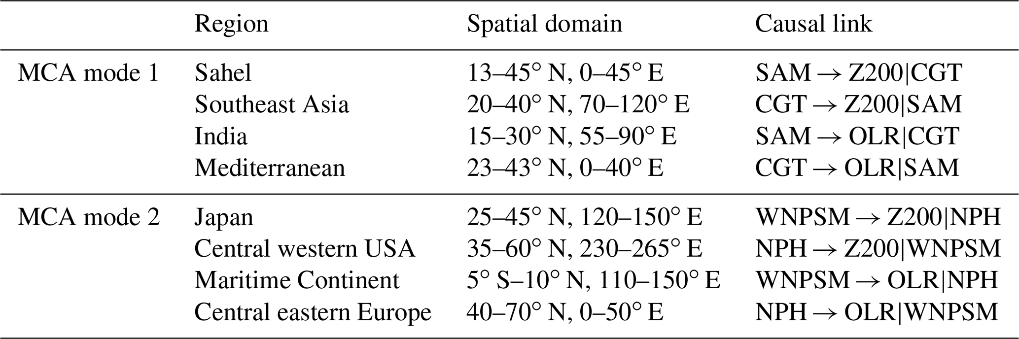
The spatial domains used to define these regions are shown in Table 3. For each region and for each sample in the 1000-ensemble member subsampling Experiment B, the causal effect is spatially averaged (accounting only for significant values; i.e. zero values are discarded as they are not significant), and the absolute value is taken after averaging. In this way, we obtain a distribution of 1000 β values for each region of interest. Note that we choose to consider spatially averaged absolute β values as indicators for corresponding teleconnection strength to focus on the strength of the causal effect rather than the number of significant grid points or the sign of the connection. Probability density functions (PDFs) for the subsampling results of each β value (one for each of the eight regions in Table 3) are estimated, and the reference β values calculated in ERA-S are shown as magenta vertical lines in each PDF in Figs. 8 and 9. We do not show the reference β values for ERA-L as those are calculated with a larger number of years and would not represent a fair benchmark to compare them with β values obtained from a different set of years.

Table 3 Spatial domains of selected regions.

For MCA mode 1, which is characterised by the SAM–CGT pair, we show that the link from the SAM to Sahel Z200 (SAM → Sahel Z200|CGT) is the one with the largest bias between SEAS5-R and ERA-S, with no subsample in our 1000-member subsampling Experiment B being capable of reproducing the ERA-S causal link strength (Fig. 8b), consistent with that shown in Fig. 6e. By contrast, the causal effect of SAM on OLR over India (SAM → India OLR|CGT) falls in the respective range of values of the 1000 subsamples, with the ERA-S β values falling between the 10th and the 90th percentile (Fig. 8f). This result is again in agreement with that shown in Fig. 5j, which depicts parts of the Arabian Sea as a region where β_SEAS5 is overestimated. Similarly, also β coefficients for the causal effect of CGT on OLR over the Mediterranean (CGT → Medit. OLR|SAM) show a good agreement between ERA5-S and SEAS5-R (Fig. 8h). Thus, in these regions the β values are compatible with those for the reanalysis data when the spread of SEAS5 β values is considered. The causal effect of the CGT towards Southeast Asia Z200 (CGT → SE-Asia Z200 | SAM) also shows a β_ERA5 falling in the middle of the β_SEAS5 distribution (Fig. 8d). However, it is worth noticing that the position of the negative causal links in Fig. 8c is displaced eastward compared to that shown in ERA5 (Fig. 3b).

Results for MCA mode 2, analysing the North Pacific high (NPH) paired together with the western North Pacific summer monsoon (WNPSM), are shown in Fig. 9. The links from the NPH towards the northwestern US Z200 (NPH → NW-US Z200|WNPSM) (Fig. 9d) and from the WNPSM towards the Maritime Continent OLR (WNPSM → M.Cont. OLR|NPH) (Fig. 9f) are those with the largest difference between SEAS5-R and ERA-S β values, with ERA-S β values falling at the upper edge of the PDF (above the 90th percentile), in agreement with what is shown in Fig. 6b and k. In contrast, the links from the WNPSM towards Japan Z200 (WNPSM → Japan Z200|NPH) (Fig. 9b) and from the NPH towards central Europe OLR (NPH → CE-EU OLR|WNPSM) (Fig. 9h) fall towards the centre of the distribution. That is, for those cases in which ERA5 values fall in the middle of the distribution, the particular modelled field is more likely to have a low bias. We again test our results for the dependence on the initialisation date of the SEAS5 dataset. Figures S10 and S11 in the Supplement show the same as Figs. 8 and 9 produced using SEAS5 initialised on 1 March. The results obtained are qualitatively and quantitatively very similar, with β values for (the same) five out of the eight analysed regions falling between the 10th and the 90th percentile consistently for both SEAS5 initialisation dates. Hence, the initialisation date does not affect the spread of the causal effect strengths in subsampling Experiment B markedly.

It should be noted again that the β values obtained in Experiment B do not refer to the same set of causal links as shown in Figs. 3, 5 and 6. Thus, we provide the same kind of information as shown in Figs. 8 and 9 also using the causal maps obtained in Experiment A (Figs. S12 and S13). In general, β values obtained from Experiment A for the analysed regions show a good agreement for MCA mode 1, where, like in Fig. 8, the link SAM → Sahel Z200|CGT shows the strongest bias with β_ERA5 falling outside the β_SEAS5 distribution (above the 100th percentile), while β values for Southeast Asia Z200, India OLR and Mediterranean OLR fall below the 90th percentile (Fig. S12). For MCA mode 2, all β_ERA5 values fall between the 90th and the 100th percentiles. Thus, the underestimation effect, which in Experiment B is limited to the NPH → NW-US Z200|WNPSM and the WNPSM → M.Cont. OLR|NPH causal maps (Figs. 8d,f), also affects causal links WNPSM → Japan Z200|NPH and NPH → CE-EU OLR|WNPSM in Experiment A (Fig. S13). These results further support that, while the spatial pattern and signs of the causal links are both fairly well reproduced in SEAS5, the underestimation of the strength of the β values is found in both Experiments A and B.

3.5 The effect of the ERA5–SEAS5 mean state bias and ENSO on tropical–extratropical causal links

We investigate how the bias in convective activity between ERA5 and SEAS5 may affect the misrepresentation of the monsoon–desert mechanism and find inconclusive results. SEAS5 shows enhanced convective activity with respect to ERA5 around the Equator (negative OLR anomalies in Fig. S14m,o) and a drier tendency over central India and the Arabian Sea (positive OLR anomalies in Fig. S14m, o). Rodwell and Hoskins (1996) have shown that the heat source provided by the convective activity in the Indian Ocean–Bay of Bengal region generates Rossby waves that reach the Sahara. However, the latitudinal position of the heat source is critical: a heat source located in the south (10^∘ N) does not act as a source of Rossby waves capable of reaching the Sahara, while a heat source located around 25^∘ N does. Thus, we investigate whether the dry bias over central India may explain low causal effect β values over the Sahel and North African region and calculate causal maps for years with enhanced convective activity over central India and for those with enhanced convective activity over the tropical Indian Ocean. Despite a certain tendency towards higher β values over North Africa being detected during years with enhanced convection over central India in SEAS5 initialised on 1 May (40 % higher compared to years with enhanced convection over the Indian Ocean; Fig. S15j), this result is not found in SEAS5 initialised on 1 March and thus remains inconclusive (Fig. S15e).

Finally, we investigate the effect of ENSO states on the sign and strength of the tropical–extratropical causal interactions shown in Fig. 4 and find that the effect of ENSO positive and negative phases on the SEAS5 dataset is mostly marginal with a few exceptions. We define Niño 3.4 positive and negative years based on seasonal (JJAS) SST anomalies averaged over the Niño 3.4 region (5^∘ S–5^∘ N, 190–240^∘ E) and calculate causal maps for the effect of SEAS5-R MCA mode 1 and 2 on the Z200 field separately for 90 Niño 3.4 positive and 90 Niño 3.4 negative years. Note that this set corresponds to those years that fall above/below the 85th/15th quantiles of SST anomalies in the Niño 3.4 region. These thresholds correspond to [+0.73 K, −0.62 K] for SEAS5 initialised on 1 March and to [+0.63 K, −0.69 K] for SEAS5 initialised on 1 May. Both pairs of thresholds are more stringent than the [+0.5 K, −0.5 K] threshold generally used in observational data. This definition allows us to have the same number of El Niño and La Niña years and thus avoid differences in the magnitude of the β values due to different sizes of each sample. Moreover, this definition is also consistent with the inherent skewness of ENSO time series, which have larger positive peaks though for the majority of the time the index is negative.

The results for SEAS5-R MCA mode 1 are shown in Fig. 10 for both Niño 3.4 positive (left column) and Niño 3.4 negative years (right column), as well as for different initialisation dates (1 March and 1 of May). Comparing the causal maps in Fig. 10 left and right column with those in Fig. 4 shows that, in general, the spatial patterns and the sign of the causal links are not affected markedly by the sign of the ENSO anomalies. A comparison of the β_niño and β_niña values with the β_SEAS5 distribution obtained from 1000 subsamples of 90 years each (consistent with the length of the El Niño and La Niña samples) is presented in Fig. S16 (see Supplement) and shows that β_niño and β_niña values tend to fall in the middle of the β_SEAS5 distribution. One noteworthy exception is presented by the β_niño and β_niña values for the SAM → Z200|CGT link in the tropical central Pacific (red cross in Fig. 10a–d). While for El Niño years, the causal effect of SAM on the tropical central Pacific is positive and markedly strong (β_niño ∼0.2–0.3; Figs. 10a, c), during La Niña years the causal effect is almost absent or weaker in strength (β_niña ∼0.1; Fig. 10b, d). In contrast, β_niño and β_niña values for the SAM → Z200|CGT link over the Maritime Continent regions (blue cross in Fig. 10a–d) show the opposite result: a strong negative causal link is found during La Niña years (β_niña $\sim -\mathrm{0.2}$; Fig. 10b, d), while during El Niño years this causal link is completely absent (Fig. 10a, c).

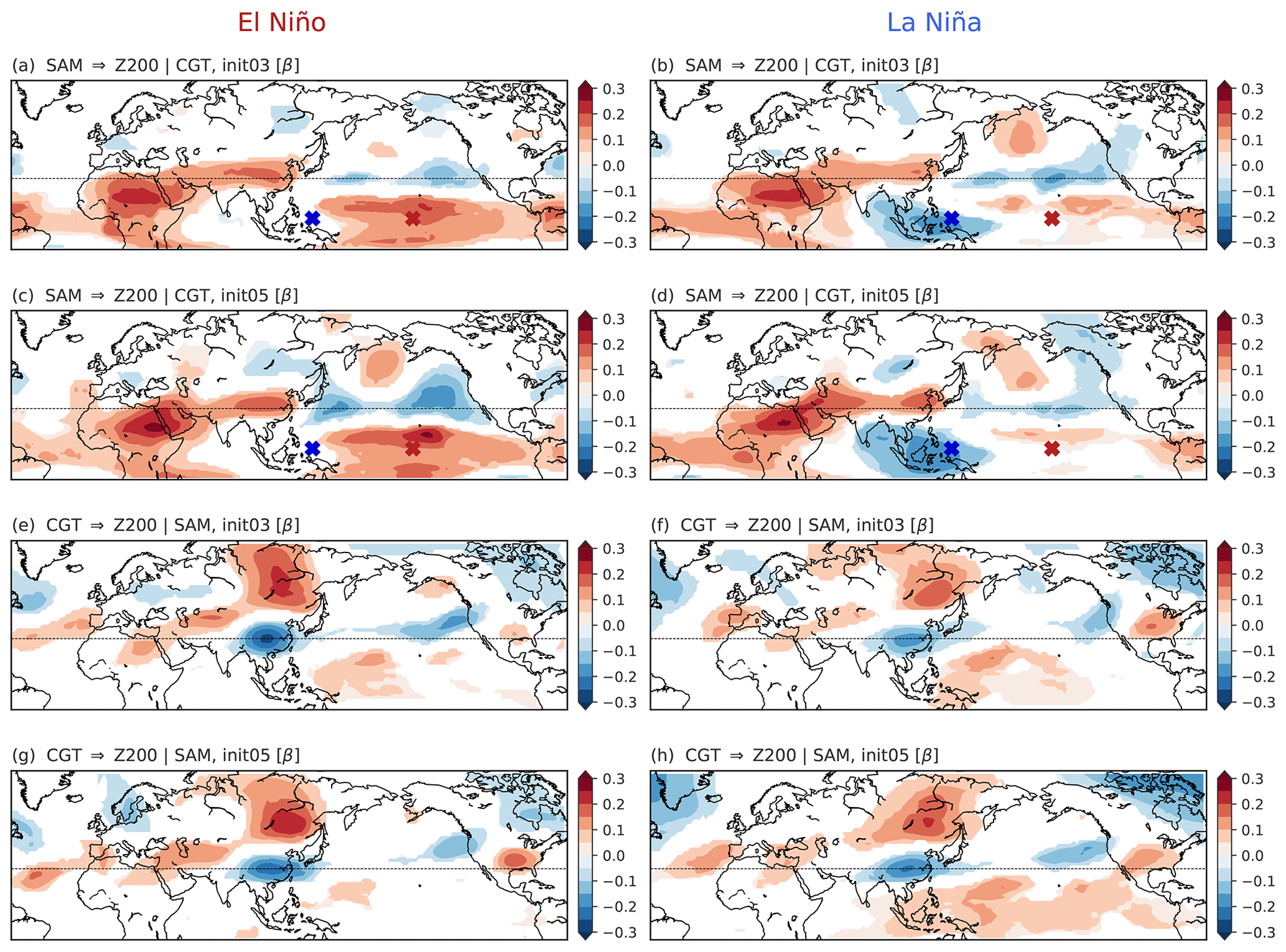
Figure 10 ENSO effect on tropical–extratropical links: MCA mode 1. Panels (a) and (b) show the causal maps for SEAS5 data initialised on 1 March for the SAM → Z200|CGT link respectively during Niño 3.4 positive and negative years. Panels (c) and (d) are the same as for panels (a) and (b) but for SEAS5 data initialised on 1 May. Panels (e) and (f) are the same as for panels (a) and (b) but for the link CGT → Z200|SAM. Panels (g) and (h) are the same as for panels (e) and (f) but for SEAS5 data initialised on 1 May. Only grid points with corrected p values significant at α= 0.05 are shown.

Causal maps for MCA mode 2 and for the ENSO years versus neutral years (i.e. analysing El Niño and La Niña years together and separating them from neutral years) are displayed in Figs. S17–S20 and show similar results. Thus, we conclude that in general ENSO does not alter the sign and spatial patterns of tropical–extratropical teleconnection qualitatively, the only exception being the ENSO region itself, where El Niño years see a more prominent causal effect over the tropical central Pacific and La Niña years over the Maritime Continent.

4 Discussion

In this work, we have provided a process-guided statistical analysis, built on causal discovery, of the representation of boreal summer tropical–extratropical intraseasonal teleconnections in the Northern Hemisphere in SEAS5 seasonal forecasts by ECMWF. We have analysed the two first modes of covariability identified using maximum covariance analysis (MCA) between weekly geopotential height (Z200) and convective activity (OLR) fields in reanalysis data from the ERA5 dataset for the period 1993–2016. The first MCA mode shows the South Asian monsoon (SAM) paired with the circumglobal teleconnection pattern (CGT), while the second MCA mode shows the western North Pacific summer monsoon (WNPSM) paired with the North Pacific high (NPH). Causal maps showing the causal effect of these four patterns on Northern Hemisphere Z200 and OLR fields at 1-week lead time for 1979–2020 (Fig. S1; see Supplement) and 1993–2016 (Fig. 3) are largely consistent with results obtained with ERA-Interim data for the period 1979–2018 (Di Capua et al., 2020a).

Here, we have focused on assessing the ability of SEAS5 seasonal forecasts in reproducing those results. To achieve this goal and provide a meaningful comparison, we have projected the first two MCA modes calculated in ERA5 onto SEAS5 data and calculated the corresponding causal maps (Fig. 4). In general, causal maps obtained with SEAS5 correctly reproduce the sign and the spatial patterns of ERA5 causal maps, though with weaker magnitudes (Fig. 4). Thus, spatial patterns shown in SEAS5 seasonal forecast causal maps are validated by those extracted from ERA5: since the SEAS5 forecasting system can qualitatively reproduce the patterns seen in ERA5 reanalysis, we gain confidence that observed causal maps represent the effect of actual physical mechanisms.

The observed commonly negative bias in causal effect strength found in SEAS5, i.e. a general underestimation of the causal effect, may arise for different reasons: (i) ERA5 causal maps are subject to multidecadal variability and/or affected by the limited time span considered or (ii) the SEAS5 forecasting system is missing and/or misrepresenting a key mechanism for a correct representation of the strength of the analysed causal links. To test the first hypothesis, we have performed a subsampling experiment, providing a thousand causal maps obtained using 24 years of randomly selecting one member for each forecast year (out of the 25 members available for each year). We have imposed the same set of causal links as observed in ERA-S (Fig. 3) and calculated the causal effect in the 1000 times subsampled SEAS5 data (Experiment A), showing that in general ∼70 % of the grid points show a β_ERA5 value above the 80th percentile of the β_SEAS5 distribution. Then, we ran the 1000-member subsampling experiment a second time but leaving it to the PCMCI algorithm to identify the causal links characteristic of SEAS5 without further constraint (Experiment B) and identified eight key regions for which we compared the observed ERA5 causal link strength with the range of SEAS5 values obtained from the subsampling ensemble (Figs. 8 and 9). Although the causal effect strengths in ERA5 are generally higher than the corresponding mean of the SEAS5 distribution, approximately half of the β coefficients for the eight analysed regions fall below the 90th percentile of the SEAS5 distribution (three out of four for MCA 1 and two out of four for MCA 2). Thus, SEAS5 has difficulty generating high values of the teleconnection strength especially over North Africa, North America and the Maritime Continent (where the ERA5 reference values exceed the SEAS5 90th percentile). In the other analysed regions, for a correct estimation of the strength of the causal links, using time series of the same length is crucial to avoid underestimation effects due to the length of the time series.

We have calculated the biases between ERA5 and SEAS5 for SST and U200 JJAS climatologies and showed that time-mean biases are present both in tropical and extratropical SST and in the mid-latitude jet over Eurasia (Fig. S14). The U200 mean-state biases in the mid-latitudes suggest a systematic northward shift of the subtropical westerly jet across Eurasia, possibly affecting the waveguide for the CGT and Silk Road patterns. Future work may employ nudging experiments to test the sensitivity to this northward shift, although previous work had shown little effect of this phenomenon on the CGT pattern (Beverley et al., 2019). Changes in the initialisation dates of the SEAS5 simulations (here 1 March and 1 May) also impact the magnitude of both SST and U200 biases, with reduced SST biases in SEAS5 data initialised on 1 May and seemingly increased biases for the Eurasian jet when compared to SEAS5 data initialised on 1 March (see Fig. S14).

In boreal summer, the CGT pattern arises even without the heat source provided by SAM (Ding et al., 2011), as it represents a preferred mode of variability of boreal summer circulation that can be ignited by different forcings (Kornhuber et al., 2020; Teng and Branstator, 2019). Recent work has shown that there is a positive causal link from the SAM to the CGT (Di Capua et al., 2020b, a). In general, climate models struggle to reproduce the climatology of SAM rainfall patterns, both in magnitude and spatial pattern (Menon et al., 2013), and SEAS5 seasonal forecasts underestimate the strength of the SAM convective activity and rainfall over the Indian peninsula and the Bay of Bengal (see Fig. S14 or Chevuturi et al. 2021). The CGT pattern has been shown to be too weak in System 4 (ECMWF's previous operational seasonal forecasting system), likely due to a dry bias in precipitation: weaker convective activity over the Indian subcontinent does not provide the heat source that reinforces the CGT pattern (Beverley et al., 2019; Ding and Wang, 2005; Di Capua et al., 2020b). If the forcing (SAM) is too weak, the response (CGT) will be too weak as well, but this does not necessarily affect the strength of the causal link. Here, our analysis shows a negative bias in β coefficients over North Africa in the first MCA mode; thus there is not only a negative bias in the precipitation over the Indian peninsula, but also the causal link strength is too weak. In general, our results also show good agreement with what was shown in Beverley et al. (2021), in which the interaction between the CGT and the SAM has been explored by applying a heating source over the Indian subcontinent in ECMWF System 4. Their results show that the heating source induced by SAM convective activity is effective at driving a CGT-like wave train in the northern mid-latitudes; however the response in the model is weak compared to the observed patterns.

Despite consistent underestimation of causal link strength in certain regions (Figs. 5 and 6), these results imply the ability of the SEAS5 forecast system to reproduce the sign and the spatial distribution of the observed causal patterns for boreal summer intraseasonal variability in the Northern Hemisphere (Figs. 4–9). Although this analysis neither relies on nor implies a skilful forecast, the causal effect of tropical and mid-latitude patterns on circulation and convection in the Northern Hemisphere in SEAS5 seasonal forecasts is qualitatively well comparable with that shown in ERA5 reanalysis. Here we have shown for which regions the agreement between SEAS5 and ERA5 is good (or for which ERA5 values at least fall in the range of values shown in the 1000-member subsampling experiments) and those for which no subsample of SEAS5 can reproduce values comparable to ERA5. The region with the strongest bias, which cannot be reproduced in SEAS5, is the Sahel region. This may be explained by the southward shift of OLR and rainfall activity towards the equatorial Indian Ocean in SEAS5, disrupting the Rossby wave-forced teleconnection pattern (Rodwell and Hoskins, 1996). However, our analysis to determine the importance of the latitudinal position of convective activity in the Indian Ocean basin is inconclusive (Fig. S15).

We further analysed the effect of the El Niño–Southern Oscillation (ENSO) on these boreal summer tropical–extratropical links in SEAS5, and we found that, in general, different ENSO phases do not affect the spatial patterns and sign of the causal links substantially (see Figs. 10 and S16–S20). However, depending on the specific region, some effect on the strength of the causal links is detected. The most prominent effect is shown in the tropical Pacific–Maritime Continent area, with causal links over these two regions that appear or disappear depending on the chosen ENSO phase (Fig. 10a–d). These findings are generally in agreement with Di Capua et al. (2020a), who showed that the spatial patterns and the sign of the causal links were mainly unaffected by ENSO; however, they noticed a regional dependence of the strength of the causal links on ENSO (see their Fig. 6). Although the effect of ENSO on the strength of the causal links seems to be marginal, we highlight those regions where a change in the strength is identified consistently both for 1 March and 1 May initialisation dates. These regions are mainly located in the tropical belt, in particular the western and central tropical Pacific (Fig. S16a–d). Similar results are found for the effect of neutral versus ENSO active years (see Figs. S19 and S20). In general, the spatial pattern and sign of the causal links do not change; however the effect of the identified MCA patterns seems to increase in the tropical Pacific during neutral years, likely due to the absence of a strong ENSO signal. These results align with the findings of Goddard and Dilley (2005), who showed that the active phase of ENSO does not affect the numbers of extremes but their overall predictability. Nevertheless, as discussed above, a change in the forcing (e.g. stronger convective activity induced by ENSO) would still result in a stronger effect even if the (relative) causal effect does not change.

This information becomes even more relevant in the context of climate change. If EC-Earth (Döscher et al., 2022) (the Earth system model built by the ECMWF which uses the same atmosphere model as SEAS5) behaves similarly to ERA5, we can gain some confidence that at least the sign and spatial patterns of these tropical–extratropical teleconnections are well represented, though the strength of the links shows a large spread (Figs. 8 and 9). Future work will analyse how these teleconnections change in future projections under global warming scenarios. The analysed regions (from the South Asian monsoon to the North American and Eurasian continents) are prone to suffering effects of ongoing anthropogenic climate change (Pfleiderer et al., 2019; Mann et al., 2018; Coumou et al., 2018, 2017; Huntingford et al., 2019; Turner and Annamalai, 2012). Therefore, it is critical to evaluate a model's ability at reproducing key seasonal modes of variability and in doing so, identify key targets for model development and motivate the improvement of parameterisation schemes. Ultimately, this could lead to increased reliability of seasonal and subseasonal forecasts: helping in improving warning systems and taking sensible early action to protect economy and society in the most vulnerable regions, especially for boreal summer, when the effect of climate change is felt the most (Christidis et al., 2014; Teng and Branstator, 2019; Kornhuber et al., 2020; Coumou et al., 2015, 2017).

Finally, this process-based validation analysis represents a step towards the implementation of hybrid forecasts that combine statistical with dynamical models to increase the skill of seasonal and subseasonal weather forecasts (Schepen et al., 2012). By identifying the regions where a certain pattern exerts a significant influence and/or deriving information on which regions have a bias in the model, we provide useful information on the regions where the model representation of these mechanisms should be improved and work towards targeted forecasts. Moreover, general circulation models show higher skill at forecasting tropical atmospheric dynamics than in the mid-latitudes or high latitudes (Shukla, 1998; Chen et al., 2015); thus, knowing which regions in the Northern Hemisphere are more affected by tropical precipitation (as shown in Fig. 4) provides valuable information to improve seasonal forecast skill.

5 Conclusions

In summary, this analysis has shown that ECMWF's seasonal forecasts have good ability at reproducing the sign and the spatial patterns of the causal effect of the two main modes of covariability between tropical convection and mid-latitude circulation in boreal summer in the Northern Hemisphere. Despite a general underestimation of the causal link strength, a subsampling experiment has shown that, in most of the analysed regions, this negative bias is actually contained in the spread of the SEAS5 seasonal forecasts. Thus, our confidence in the ability of the SEAS5 forecasting system to qualitatively correctly represent those causal links identified in ERA5 reanalysis is increased. The effect of different ENSO phases (or active ENSO versus neutral years) on tropical–extratropical links seems to be marginal, although biases in the SEAS5 model (e.g. too weak convective activity in the SAM region) may explain this discrepancy with observations. Further work is needed to confirm these results and their implications. Finally, the causal links represented in these causal maps represent a starting point to produce a new family of hybrid statistical model-based forecasts. In conclusion, this analysis has shown the usefulness of causal discovery algorithms as a tool for providing process-guided statistical validation of general circulation models and has led to increased knowledge on the effects of tropical–extratropical teleconnections in boreal summer in the Northern Hemisphere.