Predictable decadal forcing of the North Atlantic jet speed by sub-polar North Atlantic sea surface temperatures

It has been demonstrated that decadal variations in the North Atlantic Oscillation (NAO) can be predicted by current forecast models. While Atlantic Multidecadal Variability (AMV) in sea surface temperatures (SSTs) has been hypothesised as the source of this skill, the validity of this hypothesis and the pathways involved remain unclear. We show, using reanalysis and data from two forecast models, that the decadal predictability of the NAO can be entirely accounted for by the predictability of decadal variations in the speed of the North Atlantic eddy-driven jet, with no predictability of decadal variations in the jet latitude. The sub-polar North Atlantic (SPNA) is identified as the only obvious common source of an SST-based signal across the models and reanalysis, and the predictability of the jet speed is shown to be consistent with a forcing from the SPNA visible already within a single season. The pathway is argued to be tropospheric in nature, with the SPNA-associated heating extending up to the mid-troposphere, which alters the meridional temperature gradient around the climatological jet core. The relative roles of anthropogenic aerosol emissions and the Atlantic Meridional Overturning Circulation (AMOC) at generating predictable SPNA variability are also discussed. The analysis is extensively supported by the novel use of a set of seasonal hindcasts spanning the 20th century and forced with prescribed SSTs.

1 Introduction

European winter weather is strongly influenced by the variability in the North Atlantic eddy-driven jet, and it is therefore of high societal value to predict this variability as far in advance as possible. Recent studies have shown that, remarkably, retrospective ensemble forecasts (“hindcasts”) are now able to skilfully predict some components of the low-frequency variability in the winter jet at lead times of up to 10 years (Smith et al., 2019; Athanasiadis et al., 2020). However, the exact source of the predictable signal and mechanisms involved remain unclear, making it uncertain to what extent one can rely on this skill to remain for genuine decadal forecasts of the future. The aim of this paper is to try to clarify these points.

In Simpson et al. (2018), by considering a jet index based on zonal winds at 700 hPa, it was shown that the decadal variability in the jet is much stronger in March than in the boreal winter months of December, January, and February (DJF). This late winter jet variability was argued to arise from the internally generated component of Atlantic Multidecadal Variability (AMV) in North Atlantic sea surface temperatures (SSTs), though the mechanisms were not elucidated; they also showed that models failed to capture the connection. In alignment with the enhanced decadal variability, the observed connection between the AMV and the jet was shown to be far greater in March than during DJF. Nevertheless, Smith et al. (2019) and Athanasiadis et al. (2020) showed that skilful decadal forecasts of the DJF-averaged North Atlantic Oscillation (NAO) could be achieved, and the latter suggested that the skill appeared to be driven by the AMV. Both Smith et al. (2019) and Athanasiadis et al. (2020) emphasised an apparent “signal-to-noise paradox” in these forecasts, mimicking the phenomenon observed for seasonal winter NAO forecasts (Scaife and Smith, 2018). This “paradox” effectively says that the real world appears to be much more predictable than the forecast model thinks it is, with the model underestimating the response to forcing or the response to predictable boundary conditions on seasonal-to-decadal timescales relative to the unpredictable noise. A practical consequence of this behaviour is that models are likely underestimating the predictable component of decadal winter jet variability, suggesting that the results of Simpson et al. (2018) and Athanasiadis et al. (2020) are consistent with a hypothesis that the AMV is driving predictable decadal jet¹ variability from December through March. In fact, several studies have found that even the total decadal variability appears to be systematically underestimated in models (Kravtsov, 2017; Wang et al., 2017; Kim et al., 2018; Simpson et al., 2018; Bracegirdle, 2022).

Numerous studies have been conducted on the potential for air–sea coupling to generate links between the AMV and the jet, starting with the pioneering work of Bjerknes (1964). The decadal variability in the AMV itself has been hypothesised to be driven by a combination of the Atlantic Meridional Overturning Circulation (AMOC) (Bjerknes, 1964; Delworth et al., 1993; Kushnir, 1994), anthropogenic aerosols and other greenhouse gases (Booth et al., 2012; Bellomo et al., 2018; Robson et al., 2022), and stochastic atmospheric forcing (Hasselmann, 1976; Clement et al., 2015; O'Reilly et al., 2019b). An excellent recent overview on these topics with more complete references can be found in Zhang et al. (2019). Different mechanisms have been put forward for how the AMV affects the jet, including the direct modulation of low-level baroclinicity and stationary waves by the North Atlantic SST anomalies (Kushnir, 1994; Msadek et al., 2011; Kushnir et al., 2002; Peings et al., 2016), forcing from the tropical Atlantic (Davini et al., 2015), and stratospheric pathways (Omrani et al., 2014). However, the response in climate models to imposed AMV anomalies appears inconsistent and model dependent (Ruggieri et al., 2021), and the period of highly reliable observational data is short, making it challenging to distinguish between different hypotheses.

One major source of uncertainty in and across many studies is that the decadal variability is an average over several different processes occurring on different timescales due to (a) the continuous nature of air–sea coupling and (b) the fact that the AMV pattern itself evolves over time, with the anomalies in the sub-polar North Atlantic (SPNA) arising first before propagating towards the tropical Atlantic (Zhang et al., 2019; Wills et al., 2019). This makes it difficult to attribute causality between atmospheric vs. oceanic forcing and makes it unclear how to interpret the presence of multiyear lags in AMV–NAO links, such as the result that the AMV appears to force the NAO most strongly when leading by around 10 years (Peings and Magnusdottir, 2014a; Kwon et al., 2020). Furthermore, it becomes challenging to distinguish between the role played by particular regions in the Atlantic Ocean, such as the sub-polar vs. tropical North Atlantic. However, several studies have emphasised the importance of the SPNA in particular (Gastineau and Frankignoul, 2015; Woollings et al., 2015; Ortega et al., 2017; Wills et al., 2019), especially on longer timescales (Delworth et al., 2017).

In this paper, we make crucial use of two techniques to help address these challenges:

1. the separation of the eddy-driven jet into two components, corresponding to the speed and latitude of the jet;

2. the use of two seasonal hindcast ensembles, named ASF20C and CSF20C, spanning the period 1900–2010 (ASF20C is forced with prescribed, observed boundary conditions (Weisheimer et al., 2017), while CSF20C is fully coupled (Weisheimer et al., 2020); more details in Sect. 2.1).

The first point is motivated by the fact that the variability and sensitivity of the latitude and speed of the jet are very different. The jet latitude exhibits multimodality and considerable variability on seasonal timescales but shows no significant variability on decadal timescales beyond white noise (Woollings et al., 2010, 2014). The jet speed, on the other hand, is approximately Gaussian across all timescales and exhibits robust decadal variability (Woollings et al., 2014). Furthermore, Baker et al. (2017) showed that the latitude and speed respond differently to thermal forcing, and Woollings et al. (2015) showed that the processes responsible for latitudinal shifts in the jet clearly differ from those responsible for changes to the jet speed. This means that analysis based on single indices which amalgamate the latitude and speed (such as the NAO index) may struggle to identify robust links between the jet and SST anomalies. This approach has also recently been taken in Marcheggiani et al. (2023) using a complementary set of decadal forecasts.

To motivate the second point, we note that existing decadal forecasts only go back to 1954 at the earliest, leaving them with a relatively small effective sample size once any low-pass filtering or decadal averaging has taken place. The period 1954 to present also does not adequately sample the variability associated with the AMV and the AMOC. There is therefore great value in extending the analysis back to 1900. While taking decadal averages of a seasonal hindcast obviously does not constitute an actual decadal forecast, it nevertheless turns out to be useful to think of it as being like a “nudged” forecast, where both the atmospheric and oceanic state are being nudged back towards observations at the start of each winter (and moreover, for ASF20C, the SSTs are being forecasted perfectly). We will show that in fact the decadal variability reproduced by the seasonal hindcasts completely matches the predictable decadal variability in a genuine decadal forecast ensemble, justifying this perspective post hoc. This not only allows us to confidently use ASF20C–CSF20C to extend our analysis back to 1900 but also introduces two considerable benefits: the lack of coupling in ASF20C simplifies the question of causality between ocean and atmosphere, and the fact that the forecasts making up ASF20C–CSF20C only cover a single season simplifies the question of timescales.

We will show that on decadal timescales there is no predictability of the latitude of the jet and that all the observed skill at predicting the winter NAO arises from the predictability of the speed of the jet. By comparing observations with the ASF20C–CSF20C seasonal hindcasts and the Decadal Prediction Large Ensemble (DPLE) decadal forecasts (Yeager et al., 2018), we argue that predictable forcing of the jet speed arises from SST anomalies in the SPNA. Furthermore, we argue that the predictable forcing occurring on decadal timescales arises as the accumulation of a smaller forcing taking place on seasonal timescales, with no need to consider multiyear lags. Finally, we argue that the response of the jet speed to SST anomalies in the SPNA can be understood simply as the adjustment of the jet to changes in the tropospheric meridional temperature gradient across the climatological jet core.

2 Data and methods

2.1 Data

2.1.1 ERA20C

We use the 20th century reanalysis dataset ERA20C, spanning 1890–2010, as our observational “truth” (Poli et al., 2016). This reanalysis is constructed using a cycle of the Integrated Forecast System (IFS) forecast model and is made up of consecutive 1 d forecasts with data assimilation. Due to differences in available observations between the beginning and end of the 20th century, the atmospheric component of ERA20C only assimilates surface pressure in order to maintain coherence over the whole period. Both ocean and sea–ice boundary conditions come from the HadISST2.1.0.0 dataset (Rayner et al., 2003). Although it is known that the internal variability is underestimated in the early 20th century (Dell'Aquila et al., 2016), ERA20C constitutes a reasonable reference for the status of the North Atlantic climate.

2.1.2 ASF20C and CSF20C

The ASF20C model data considered come from an atmosphere-only seasonal hindcast experiment covering the 20th century (Weisheimer et al., 2017). A 51-ensemble-member seasonal forecast is initialised every 1 November from 1901 to 2010 and allowed to run for 4 months, thereby producing a December–January–February (DJF) prediction for every year in this period. The model used is version CY41R1 of the IFS. Its spectral resolution is TL255, corresponding to roughly 80 km grid spacing near the Equator, with 91 levels in the vertical. The model is run in atmosphere-only mode with prescribed observed sea surface temperatures (SSTs) with boundary conditions and initial conditions from ERA20C. Further details can be found in Weisheimer et al. (2017).

We will additionally make use of the CSF20C hindcast. This hindcast is identical to ASF20C except that it is run with dynamic coupling between the atmosphere, ice, and the ocean and is initialised using the coupled reanalysis CERA20C (Laloyaux et al., 2018). The configuration is described in Weisheimer et al. (2020) and is similar to the SEAS5 operational seasonal forecast at the European Centre for Medium-range Weather Forecasts (Johnson et al., 2019). The ocean model used is NEMO version 3.4 (Madec and the NEMO team, 2016), and the ice model is LIM2 (Fichefet and Maqueda, 1997). Both are run at a 1^∘ horizontal resolution, with NEMO using 42 vertical levels.

2.1.3 Decadal Prediction Large Ensemble (DPLE)

DPLE is made up of a suite of 40-ensemble-member forecasts, each initialised on 1 November and run for 10 years. Forecasts are initialised every year from 1954 to 2015. The forecasts are run using CESM version 1.1 using the same model and component configuration as that used in the CESM1 large ensemble (Kay et al., 2015). The atmosphere component is version 5 of the Community Atmosphere Model (CAM5; Hurrell et al., 2013), with a horizontal resolution of around 1^∘ and 30 levels in the vertical. The ocean component is version 2 of the Parallel Ocean Program (Danabasoglu et al., 2012), and the sea ice model is version 4 of the Los Alamos National Laboratory (LANL) Community Ice Code (Hunke et al., 2010). Both are run at a 1^∘ spatial resolution, with 60 vertical ocean levels. Further details can be found in Yeager et al. (2018).

To be consistent with CSF20C–ERA20C we restrict analysis to the overlapping period 1954–2010. When assessing the decadal forecast skill of DPLE, we always take averages over the entire 10-year period. For example, suppose we have a time series J made up of DJF averages of some quantity in reanalysis, and we want to assess the capacity of DPLE to predict $\stackrel{\mathrm{‾}}{J}$, where the overline denotes the average across the 10 winters from November 1954 to February 1964. Then the DPLE forecast of $\stackrel{\mathrm{‾}}{J}$ is taken to be the ensemble mean over $\stackrel{\mathrm{‾}}{x_k}$ (k=1, …, 40), where the x_k values are the 10-year forecasts initialised on 1 November 1954, with k referring to ensemble member. By doing this for consecutive 10-year periods we obtain estimates of the decadal variability predicted by DPLE which we can correlate with the observed decadal variability.

Importantly, we do not perform any drift correction of any kind in our analysis. The main goal of this paper is to understand how the atmosphere responds to decadally varying SSTs, and this can be assessed in DPLE irrespective of any drift taking place. Furthermore, it is not customary to de-drift seasonal forecasts, so no drift correction is done for ASF20C–CSF20C; not de-drifting DPLE therefore makes the analysis more directly comparable between the forecast products. For DPLE we will only ever consider two timescales: the response taking place in the first season or the 10-year mean across the whole forecast period. The drift taking place in the former is small, and the imprint of the drift in the latter is smoothed out by the large averaging window. Finally, we note that Athanasiadis et al. (2020) found that robust decadal NAO forecast skill can be diagnosed in DPLE irrespective of whether drift correction is carried out or not.

2.1.4 EC-Earth3 data

We will make use of two piControl CMIP6 (500- and 603-year long) integrations from EC-Earth3 (Döscher et al., 2022). These simulations are atmosphere–ocean coupled runs with pre-industrial forcings. These simulations are specifically interesting owing to their large internal variability induced by an internally driven centennial oscillation of the AMOC (Meccia et al., 2022), and we will use them to assess the potential role of the AMOC.

2.2 Methods

2.2.1 Metrics

The NAO index is computed as the leading empirical orthogonal function (EOF) of daily de-seasonalised DJF 500 hPa geopotential height anomalies in the Euro-Atlantic sector (30–90^∘ N, 80^∘ W–40^∘ E). A seasonal cycle is estimated by taking the average daily NAO value for each day in DJF across all years available; this cycle is then removed. When computing the NAO index for ensemble forecast data, all the ensemble member data are used to compute the EOF, after which each member's geopotential height field is projected onto the EOF pattern to obtain the individual NAO indices. The time series is not standardised further.

To compute indices of the jet speed and latitude, we follow the simplified methodology of Parker et al. (2019). Wind fields are first interpolated to a regular 1^∘ grid. Daily DJF 850 hPa zonal winds are then restricted to the region 15–75^∘ N, 60–20^∘ W and smoothed with a 5 d running mean. For any given day, the jet is said to be located at the latitude where the magnitude of the zonally averaged winds in this region is maximum. The two indices will be referred to as JetSpeed and JetLat for short. The jet latitude on that day is precisely this latitude, while the jet speed is the magnitude of the maximum. As with the NAO, a seasonal cycle is removed.

An “SPNA” index measuring SST variability in the sub-polar North Atlantic is also used extensively. This is defined as the DJF-averaged SSTs, averaged over the region 49–57^∘ N, 50–25^∘ W. The motivation for this precise choice is given in the main text. The results are not sensitive to small shifts in this region.

A more standard AMV index is also computed for comparison with the SPNA index. DJF SSTs in the North Atlantic domain 0–70^∘ N, 80–0^∘ W are detrended at every grid point; the first empirical orthogonal function of the resulting field is the standard AMV “horseshoe” pattern, and we thus take the corresponding principal component to be our AMV index.

Note that we do not remove linear trends from any of these time series. The question of whether and how to isolate internal variability in the AMV and related time series is not entirely clear (Deser and Phillips, 2021), and trends in the SPNA and jet speed time series we primarily consider here are small (e.g. around −0.5 % yr⁻¹ on average for the SPNA), with the decadal variability dominated by the oscillations that are characteristic of internal variability. Removing the trends is thus found to have no impact on the analysis (e.g. conclusions drawn concerning significance).

2.2.2 Statistics

Our default stance on significance testing is to explicitly specify a statistical model representing the null hypothesis and then generate significance thresholds by making 10 000 random draws using the model; all tests carried out in this way are two-sided. Because the motivation behind the choice of each statistical model depends on the situation at hand, we introduce each such model in the main text as and when it is required. However, we note that when modelling SSTs we generally make use of the “Fourier phase shuffle” method (Ebisuzaki, 1997). This method can be loosely described as follows. First compute the Fourier transform of the time series of interest. Second, for each Fourier mode, replace the computed phase by a randomly chosen one. Third, convert the resulting Fourier series back to a time series. The resulting randomly generated time series is guaranteed to have the same autocorrelation (at all lags) and degrees of freedom as the original time series, which is important given the considerable autocorrelation present in the SST time series we will be examining. In particular, a null hypothesis modelling SSTs in this way will typically produce much stricter significance thresholds than those that model SSTs using an AR1, which only specifies the autocorrelation at lag 1.

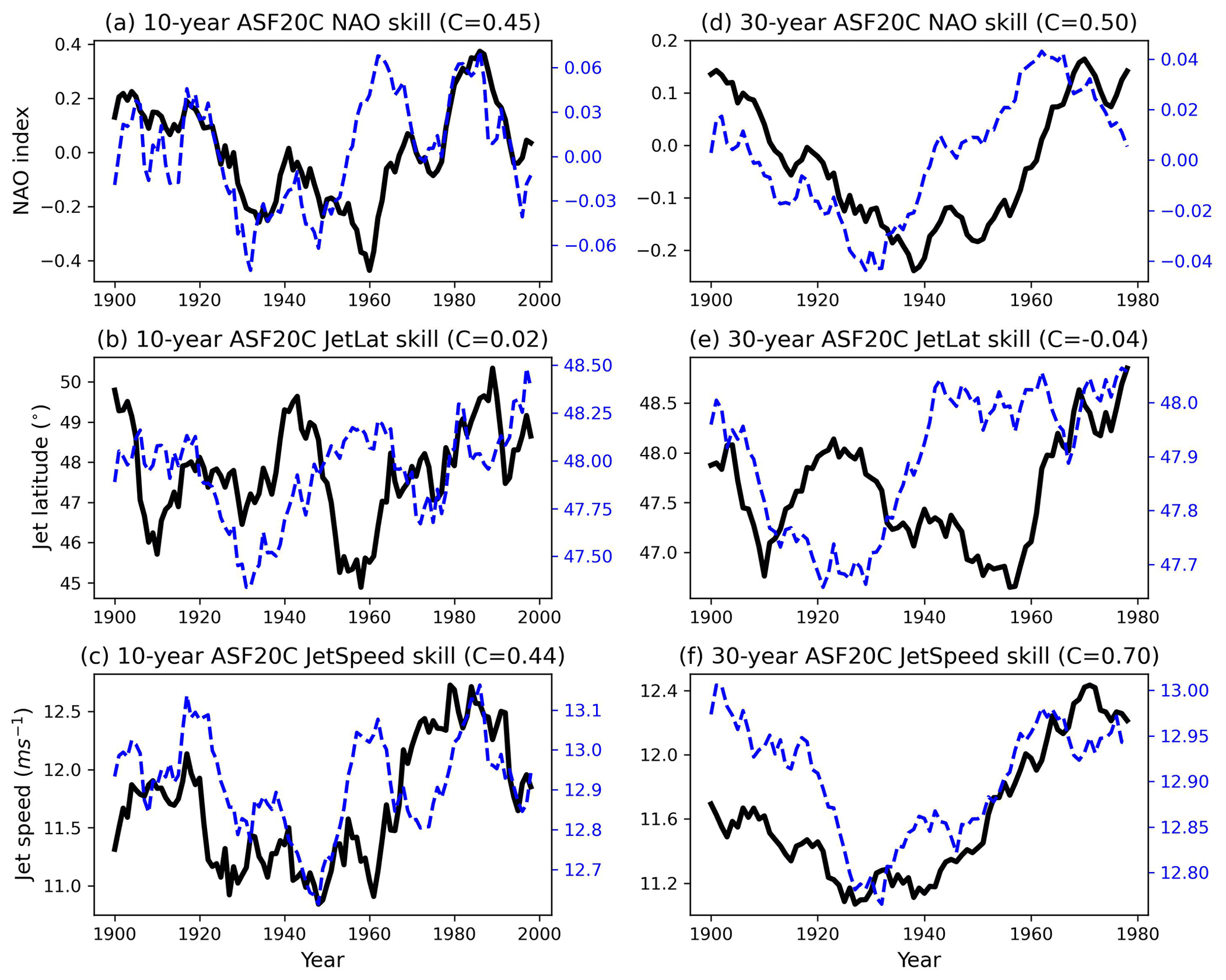
Figure 1 Time series of 10-year DJF running means of (a) the NAO, (b) the jet latitude, and (c) the jet speed. (d)–(f) The same but with 30-year running means. The thick black curves are always ERA20C, and the dashed blue curves are always the ASF20C ensemble mean. Note the different y axes for the black and blue curves. The value C in each subplot is the correlation between the two time series.

3 Predictable jet variability in ASF20C and DPLE

3.1 Predictability of the jet speed and not the jet latitude

We first examine what low-frequency jet variability is skilfully reproduced by ASF20C. Figure 1 shows 10- and 30-year running means of the NAO, jet latitude, and jet speed for ERA20C and the ASF20C ensemble mean. One aspect of the signal-to-noise paradox is that the ASF20C ensemble mean standard deviation is considerably smaller than that of ERA20C; this can be seen here by comparing the magnitudes of the two y axes, which highlight that the standard deviation in ERA20C is around 4–5 times greater than that of the ensemble mean. It can be seen that ASF20C skilfully reproduces decadal NAO variability across the entire period 1900–2010, with a correlation coefficient of ∼0.4–0.7 depending on the choice of smoothing; using the raw seasonal data gives a correlation of 0.21. The correlations obtained using 10-year smoothing closely match those reported in Smith et al. (2019) and Athanasiadis et al. (2020) using genuine decadal forecasts, suggesting that the decadal forecast skill they reported might extend all the way back to 1900. Figure 1 also clearly shows that ASF20C cannot skilfully reproduce decadal jet latitude variability but can skilfully reproduce decadal jet speed variability. Furthermore, if we regress out the (decadally averaged) ensemble mean jet speed from the ensemble mean NAO and correlate the residual with the observed NAO, we obtain ≈0.1 using 10-year averages and $\approx -\mathrm{0.1}$ using 30-year averages. Therefore, the majority of the skill that ASF20C has at reproducing decadal NAO variability is related to the jet speed. Figure S1 in the Supplement (SI) shows that, similarly, the coupled hindcast CSF20C has significant skill at predicting decadal variations in the speed but not the latitude.

Figure 2 shows that the same conclusion is true for the DPLE forecasts: there is no apparent predictability of decadal shifts in the jet latitude but high skill at predicting shifts in the jet speed. Note that taking 30-year means is much less sensible for DPLE, given its shorter coverage of 56 years, but these are included anyway for direct comparison with Fig. 1.

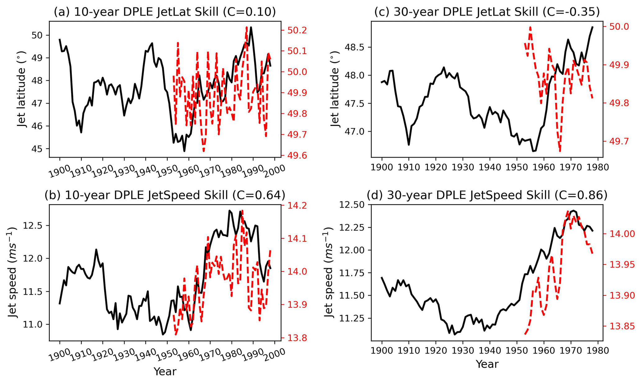
Figure 2 Time series of 10-year DJF running means of (a) the jet speed, and (b) the jet latitude. (c, d) The same but with 30-year running means. The thick black curves are always ERA20C, and the dashed red curves are always the DPLE ensemble mean. Note the different y axes for the black and red curves. The value C in each subplot is the correlation between the two time series.

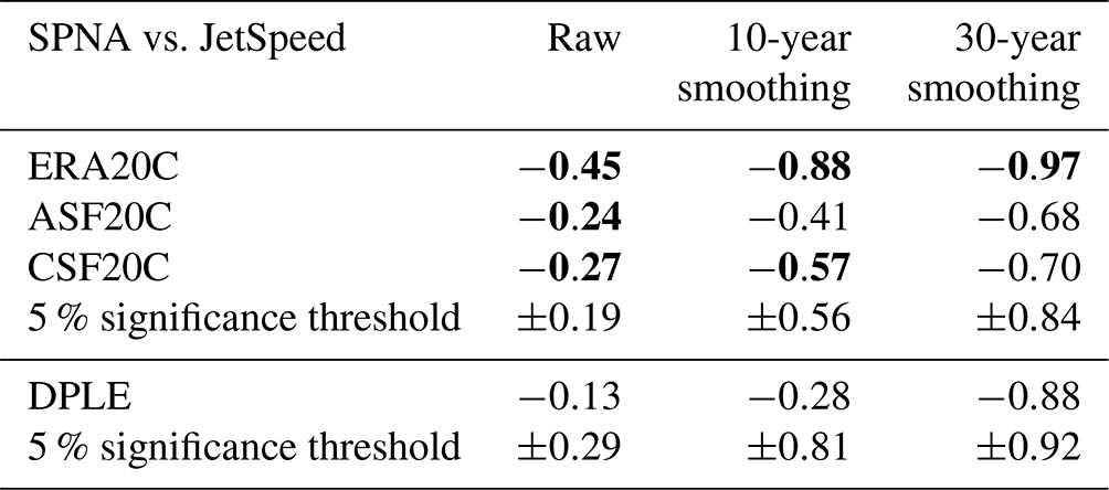
How significant are the jet speed correlations reported in Figs. 1 and 2? The 1-year jet speed autocorrelation is ≈0.0 for all three datasets, and we are therefore justified in assuming a null hypothesis of the DJF jet speed as being white noise. The approximate Gaussianity of the jet speed distribution has been previously noted (Woollings et al., 2010; Parker et al., 2019). By simulating 10 000 randomly generated DJF jet speed time series for each dataset, taking 10- or 30-year running means, and then computing correlations, we build up a distribution of correlations that can be obtained by chance. Note that taking running means will automatically introduce considerable autocorrelation to the resulting time series. Table 1 summarises the result of this significance testing. This shows that for ASF20C, whether considering 10- or 30-year smoothing, the decadal jet speed correlations are only significant to within p<0.1 and not p<0.05; the same is true for CSF20C (see Fig. S1). For DPLE, the conclusion is the same except that the correlations using 30-year smoothing appear to be significant also with p<0.05. However, as cautioned already, the small effective sample size here means that this level of confidence is probably not justified. The jet latitude correlations are never significant with respect to a similar null hypothesis, including the relatively large negative correlation emerging for 30-year jet latitude variability in DPLE ($C=-\mathrm{0.35}$).

Table 1 DJF jet speed correlations (Corr) between different datasets at different levels of smoothing. Significance thresholds assume a null hypothesis of the interannual jet speed time series being uncorrelated white noise.

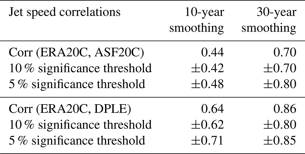
Our results here contrast somewhat with those of Smith et al. (2019) and Athanasiadis et al. (2020), which both report statistically significant decadal NAO forecasts with p<0.05. However, their significance tests differ from ours, and the smoothing they use is also very close, but not identical, to the 10-year running means we use. Table 1 shows that the 10-year ASF20C and DPLE jet speed correlations sit neatly between the bounds of the 5 % and 10 % significance thresholds, and it is therefore plausible that these differences can explain why they report a p value less than 0.05 and we do not. For this article, we will assume that ASF20C and DPLE really do have significant skill at predicting decadal variations in the jet speed.

3.2 Predictable atmospheric signals appear on interannual timescales

The similar behaviour of ASF20C and DPLE suggests that the extra information provided to ASF20C (the correct climate state every 1 November and the correct SSTs at all times) is not adding any extra jet speed skill beyond what is expected from an actual free-running, coupled decadal forecast. We interpret this as evidence for the assertion that the signals responsible for predictable decadal shifts in the jet speed are fully represented in ASF20C, and we will from now on assume that this is the case; we return to this point and alternative hypotheses later. Our assumption has two important consequences.

Firstly, since each of the 109 ASF20C winter forecasts only knows about the initial conditions and boundary forcings of the season in question, the sources of predictable decadal jet speed forcing must be present in their entirety within a single winter season. Put differently, since the atmospheric variability in ASF20C is generated by forecasts of a single season, any decadal variability ASF20C generates must arise due to atmospheric variability taking place within single seasons, even if this variability is ultimately forced by variables (e.g. SSTs) evolving on slower timescales. In particular, the predictable atmospheric signals, and the mechanisms involved, do not seem to inherently involve multiyear lags between the ocean and atmosphere or multiyear feedbacks within the atmosphere. Secondly, since the ASF20C forecasts are uncoupled, the forcing being exerted on the jet by the SSTs does not essentially depend upon atmosphere–ocean coupling in the sense that no within-season feedbacks are necessary. To the extent that there is any causal interaction between the SSTs and the atmosphere in AS2F20C, it must purely be from the former to the latter. In the sections that follow we will make use of these two points repeatedly to simplify the analysis and reasoning.

We emphasise straight away that while two-way surface coupling appears to not be required to reproduce the low-frequency jet speed variability, missing or deficient coupling may play a role in generating the signal-to-noise paradox, as suggested in Scaife and Smith (2018). It is also likely that atmosphere–ocean coupling plays a role in generating the decadal-timescale SST variability.

4 Sources of predictability from sea surface temperatures

The midlatitude troposphere broadly speaking has a decorrelation timescale of about 2 weeks (Judt, 2020), and this is also true for the daily jet speed index (not shown). This strongly suggests that the skill in both ASF20C and DPLE cannot be explained by the persistence of atmospheric initial conditions and is rather a result of forcing from some other slow-timescale process. Due to the considerable body of work emphasising the importance of SSTs in generating forecast skill, we make the assumption here that decadal jet speed skill is a result of SST forcing. The validity of this assumption is discussed in Sect. 7.1.

4.1 Sub-polar North Atlantic SSTs as a common signal across observations and forecasts

In order to locate potential sources of skill in SSTs, we compute correlations of the winter jet speed against winter SSTs at every grid point. Because of our conclusion that these sources must be visible already on seasonal timescales (see Sect. 3.2), we do this using both the raw DJF time series, as well as time series obtained by applying a 10-year running mean. Potential sources of skill are then assumed to correspond to regions of non-zero correlations that are common to ERA20C, ASF20C, CSF20C, and DPLE across both interannual and decadal timescales. While it is of course possible that the locations of signals differs somewhat across the datasets (e.g. due to biases in both the mean state and trends across the forecast models), the simplest – and more physically sound – possibility is that the signals are identical across the datasets, so we consider this possibility first.

Figure 3 shows grid point correlations for ERA20C, ASF20C, CSF20C, and DPLE at interannual timescales, while Fig. 4 shows grid point correlations of 10-year running means. Stippling indicates significance (p=5 %), where for interannual timescales the null hypothesis models the jet speed as white noise and models grid point SSTs using the Fourier phase shuffle method; on decadal timescales both the jet speed and SSTs are modelled using the phase shuffle method. At each grid point 1000 randomly generated samples from the null hypothesis are drawn in order to compute significance thresholds. Searching for commonalities across all the eight subplots by eye quickly highlights the SPNA. Already just comparing Fig. 3a and b makes this clear. A comparison with CSF20C and DPLE corroborates this and furthermore seems to rule out signals from both the tropical Pacific, tropical Atlantic, and Indian Ocean, since the correlations are opposite in sign between ASF20C–CSF20C and DPLE in these regions.

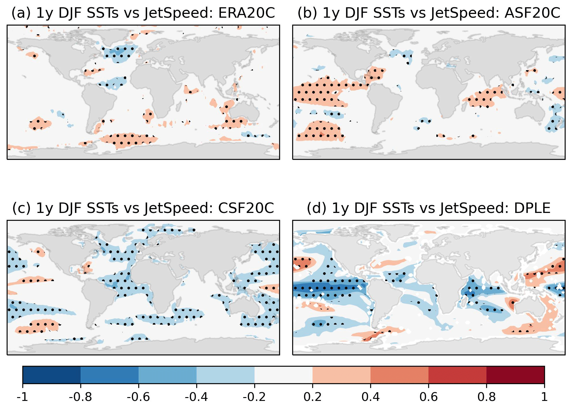
Figure 3 Correlations between the interannual DJF JetSpeed time series and DJF SSTs at each grid point in (a) ERA20C, (b) ASF20C, (c) CSF20C, and (d) DPLE. Stippling indicates significance (p<0.05); see main text for details of the null hypothesis. The period considered is 1954–2010 for DPLE and 1900–2010 otherwise.

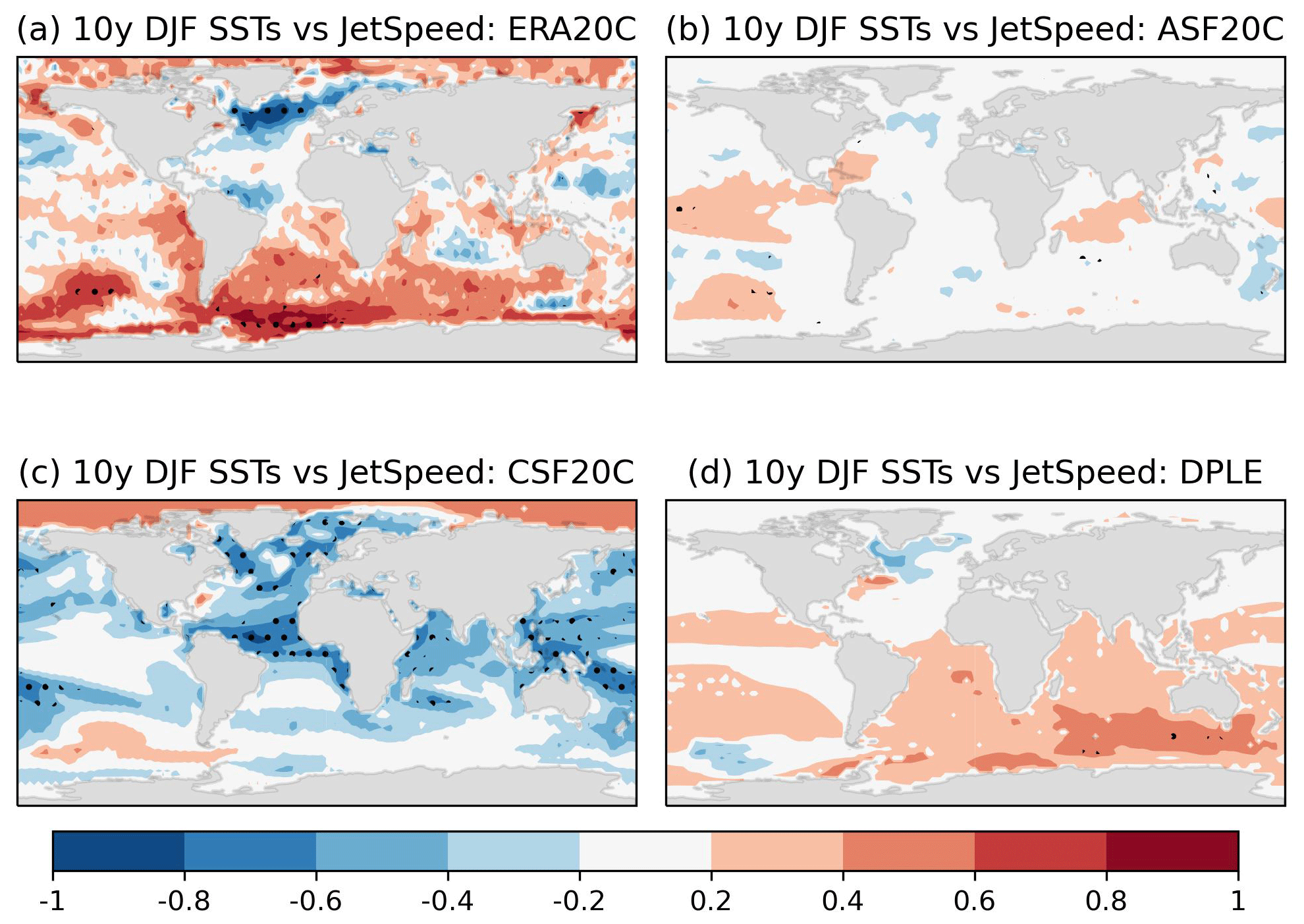
Figure 4 Correlations between 10-year running means of the DJF JetSpeed time series and DJF SSTs at each grid point in (a) ERA20C, (b) ASF20C, (c) CSF20C, and (d) DPLE. Stippling indicates significance (p<0.05); see main text for details of the null hypothesis. The period considered is 1954–2010 for DPLE and 1900–2010 otherwise.

To justify this visual inspection more objectively, we have in Fig. 5 highlighted the grid points for which all the four datasets exhibit interannual- and decadal-timescale correlations with the same sign. This makes it clear that the SPNA is the only region where spatially coherent correlations of the same sign can be found. Figures 3 and 4 show that the correlations in the SPNA region are statistically significant in five out of eight subplots, including in ERA20C across both timescales. While Fig. 5 shows a narrow strip of shared negative correlations in the tropical Atlantic, these correlations are not significant in ASF20C on any timescale and are not significant in ERA20C on decadal timescales. The correlations in this region are also close to 0 in magnitude in ASF20C on interannual timescales and DPLE on decadal timescales ($\approx -\mathrm{0.05}$ on average in both cases). Only in the SPNA are correlations of appreciable magnitude ($<-\mathrm{0.2}$) found in all datasets on all timescales. Furthermore, and crucially, the coupled DPLE forecasts have considerable skill at predicting decadal SST variability in the SPNA region but not in the tropical Atlantic (Yeager et al., 2018; Yeager, 2020).

Figure 5 Grid points where the correlations in all eight subplots of Figs. 3 and 4 have the same sign. Blue (red) grid points correspond to ones where the shared sign is negative (positive). Grid points where the sign is not consistent across all subplots have been left blank.

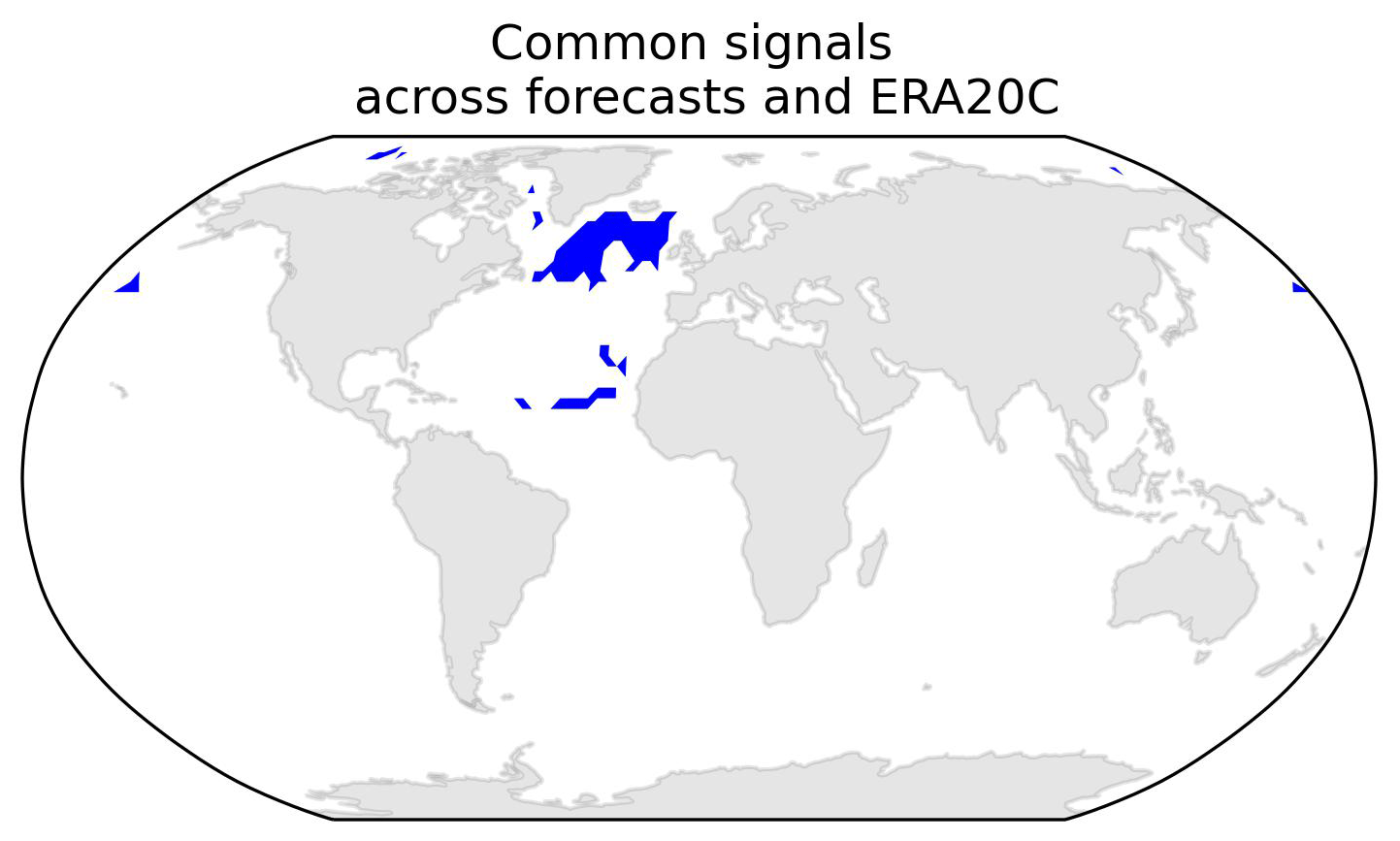
The SPNA thus emerges as a common region of interannual-to-decadal correlations between SSTs and the jet speed across ERA20C, ASF20C, CSF20C, and DPLE, and it appears to be the only such common region. We interpret this as strong evidence for the importance of the SPNA in driving decadal jet predictability. We therefore define an SPNA time series as the DJF-averaged SSTs across the domain 49–57^∘ N, 50–25^∘ W. This box was chosen because it encloses almost precisely the negative correlations highlighted in Fig. 3c in the sub-polar region. The remainder of the analysis we carry out is not sensitive to even moderately large shifts in the definition of this box, as long as the box roughly belongs to the region highlighted in Fig. 5. Other differences between the datasets seen in Figs. 3 and 4, while interesting, do not seem relevant to the study at hand and so are not discussed.

It is worth mentioning the phenomenon of false discovery rates, namely the fact that if one looks for correlations across a sufficient number of predictors, then some are bound to be significant by chance. This effect would a priori be expected to be high when considering correlations across thousands of grid points with high spatial autocorrelation. However, based on the results and discussion of previous sections, we are now assuming that (a) there is decadal forecast skill which needs to be explained and (b) this skill comes from the SSTs. A rejection of any and all grid point correlations as “false discoveries” would be directly counter to this assumption and is therefore not done. The discovery of a region of correlations common across four datasets on the other hand can be seen as providing additional evidence towards our assumption.

4.2 Significance of the SPNA–JetSpeed link

Table 2 summarises the correlations between SPNA SSTs and jet speed for the different datasets across different timescales. Figure 6 visualises the 30-year running mean time series: the sign of the SST index has been flipped for visual convenience. To generate the 5 % significance threshold reported in the table, we assume a null hypothesis that the jet speed and SPNA are uncorrelated random variables. The interannual jet speed time series is modelled as a normal distribution with no memory across years, as before. To create synthetic SPNA time series, we apply the Fourier phase shuffle method to the interannual SPNA time series in order to generate random draws that preserve the considerable autocorrelation. By correlating 10 000 such synthetic time series, along with those obtained by applying a 10- or 30-year smoothing, we can then numerically estimate the 5 % significance threshold. Note that the confidence intervals for ERA20C, ASF20C, and CSF20C were found to be almost identical, so we only report a single confidence interval encompassing all three, obtained by taking the average across the three individual intervals.

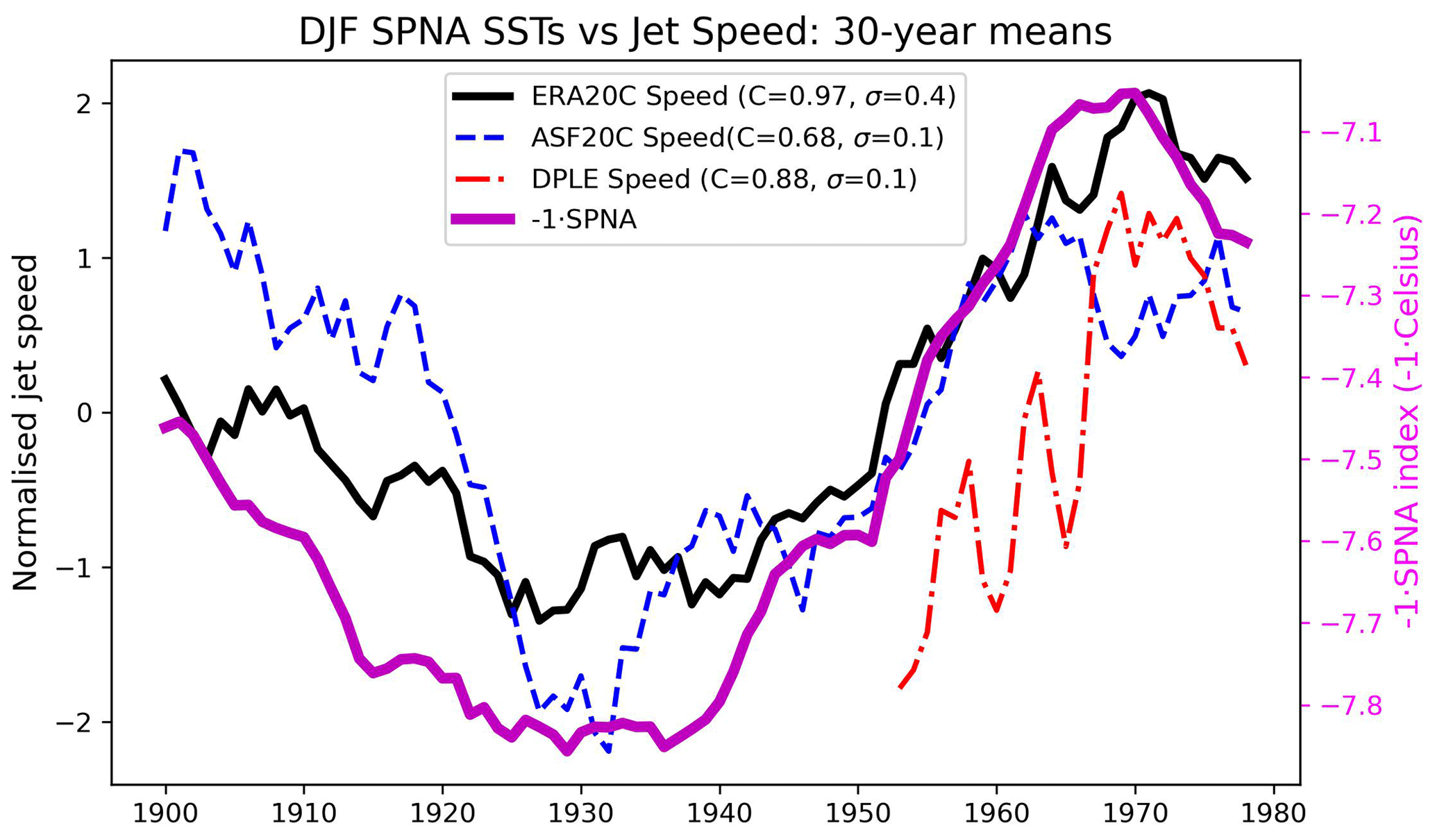
Figure 6 Time series of 30-year running means of ERA20C SPNA SSTs (thick purple: the sign has been flipped for visual convenience), ERA20C jet speeds (thick black), ASF20C ensemble mean jet speeds (dashed blue), and DPLE ensemble mean jet speeds (dashed red). The values of C in the legend indicate the correlation between the jet speed time series and the relevant SPNA time series, and the values of σ indicate the standard deviations of the jet speed time series. Note the different y axes for the jet speed and SPNA time series. The jet speed indices have all been normalised to have mean 0 and standard deviation 1.

Table 2 Correlations between DJF-averaged SPNA SSTs and DJF-averaged jet speed at different levels of smoothing. The 5 % significance thresholds shown use the null hypothesis described in the main text. Significant correlations are highlighted in bold.

The correlation between SPNA and the jet speed is highly significant in ERA20C for all timescales considered here, suggesting a robust physical link between these quantities. Both ASF20C and CSF20C have significant correlations on the interannual timescale and CSF20C also for 10-year timescales. The other correlations obtained do not pass the threshold. Of course, the lack of consistent statistical significance at 5 % does not mean the physical link in ERA20C is not simulated by the forecast models but only that these correlations would not be sufficient to establish such a link when viewed in isolation. As emphasised in Shepherd (2021), it is crucial to include physical reasoning and prior knowledge when drawing conclusions about significance. We return to this, and the question of causality, in the Discussion section.

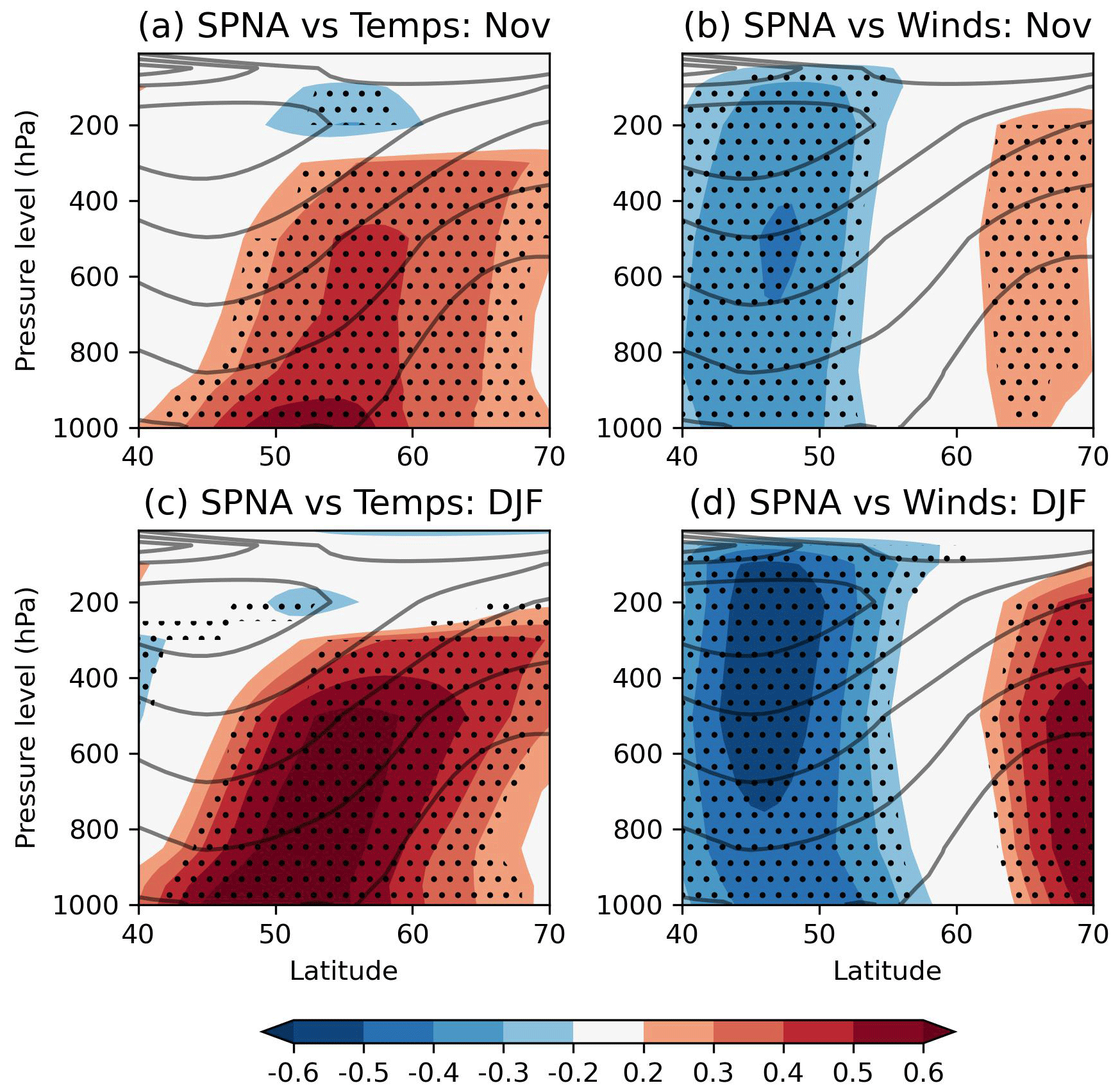
Figure 7 Correlations in ERA20C between SPNA SSTs and (a, c) zonally averaged air temperatures at different pressure levels and (b, d) zonally averaged zonal winds at different pressure levels. November averages are used in (a) and (b), while DJF averages are used in (c) and (d). The period 1900–2010 is used. The climatological zonal winds are shown in grey contours. Stippling indicates significance (p=5 %); see main text for details.

5 Pathways and timescales

5.1 The tropospheric pathway from sub-polar North Atlantic SSTs to the jet speed

When studying the impact of imposed temperature anomalies on the jet in a dry model, Baker et al. (2017) argued that much of the response could be understood simply in terms of changes to the meridional temperature gradient. This suggests a simple explanation for why the SPNA forces the jet in keeping with the analysis of Woollings et al. (2015): anomalously cold SSTs in the SPNA cool the atmosphere aloft, thereby strengthening the local meridional temperature gradient around the jet, causing an intensification of the eddies and thereby an increased jet speed. This is similar for warm anomalies but with the opposite sign. To strengthen the case for this pathway, Fig. 7 shows the vertical extent of the anomalies associated with SPNA SSTs in ERA20C by correlating November SPNA SSTs with zonally averaged (a) temperatures and (b) zonal winds at different pressure levels; the averaging is done over longitudes 60^∘ W–20^∘ E. Significance at 5 % (indicated by stippling) uses a null hypothesis which models the SPNA using the Fourier phase shuffle method and temperatures and winds as white noise. Figure 7c and d show the same but using DJF means. Figure 7a and c suggest that temperature anomalies do not remain confined to the surface but extend up to around 300 hPa, making the robust impact on the jet seen in Fig. 7b plausible. For completeness, the reverse link from the jet speed to temperatures and winds is shown in Fig. 8. Figure 8a shows that the temperature anomalies associated with the jet are maximal in the mid-troposphere. The temperature anomalies associated with the SPNA (Fig. 7a and c) project well onto the jet pattern but are maximal at the surface. Comparing Figs. 7d and 8b confirms that the association between the SPNA and the zonal winds projects onto the jet speed signature.

Figure 8 Correlations in ERA20C between jet speeds and (a) zonally averaged air temperatures at different pressure levels and (b) zonally averaged zonal winds at different pressure levels. DJF averages are used in both. The period 1900–2010 is used. The climatological zonal winds are shown in grey contours. Stippling indicates significance (p=5 %) with respect to a two-tailed t test.

Detailed analysis of the tropospheric response to an SST anomaly in the North Atlantic, such as in Deser et al. (2007), shows that the response generally proceeds in two stages. To begin with, the induced anomaly is baroclinic in nature and localised to the heat source. In the second stage the baroclinic anomalies are removed by eddy heat and momentum transport, leading to a relatively barotropic structure with a more hemispheric scope. Figure 7 shows that in DJF, the structures are relatively barotropic in nature, consistent with this tropospheric pathway having taken place. Note that this approximately barotropic structure is also visible when plotting regression coefficients instead of correlations (not shown).

To further test the importance of the tropospheric heating anomalies over the SPNA, we will compute a crude estimate of what ERA20C jet speed anomalies are expected purely from SPNA variability using geostrophic wind balance. Concretely, we will estimate the jet speed variability expected from the following assumptions:

• First is that the local meridional temperature derivative at the jet core can be completely approximated using the difference in temperatures between the jet core and the SPNA region (which sits on the northern flank of the jet). In particular, we assume that the gradient between the southern flank and the jet core does not contribute to the local derivative.

• Second is that the only air temperature variability which takes place in the period 1900–2010 is that in the atmosphere above the SPNA. In particular, temperatures above the jet core are assumed to be constant in time.

We emphasise that these are strictly stronger assumptions than standard geostrophic balance, and it is therefore not obvious, a priori, that these assumptions should suffice to accurately reconstruct jet speed variability.

To proceed, we define a region labelled “South” by 35–43^∘ N, 75–40^∘ W and a region labelled “North” using the same domain as the SPNA. The South region is chosen because it roughly encompasses the climatological core of the jet in ERA20C (not shown). We then assume a constant layer thickness between 1000 and 300 hPa, where 300 hPa is the upper limit of the heating associated with the SPNA, as seen in Fig. 7c. Let ${\widehat{T}}_{\mathrm{N}}$ and ${\widehat{T}}_{\mathrm{S}}$ denote the layer-averaged DJF air temperature between 1000 and 300 hPa in the North and South regions. By regressing our SPNA SST time series against ${\widehat{T}}_{\mathrm{N}}$, we obtain the SPNA-driven component which we denote by ${\widehat{T}}_{\mathrm{N}}$(SPNA). We let [${\widehat{T}}_{\mathrm{S}}$] denote the average of ${\widehat{T}}_{\mathrm{S}}$ across all years from 1900–2010. The time series of the difference ${\widehat{T}}_{\mathrm{N}}\left(\mathrm{SPNA}\right)-\left[{\widehat{T}}_{\mathrm{S}}\right]$ thereby roughly measures the layer-averaged meridional temperature gradient across the jet core purely associated with SPNA SST variability. Given our two assumptions, geostrophic balance with a constant layer thickness now relates this gradient to the zonal winds U_jet in the jet core according to

$$\begin{array}{}\text{(1)}& U_{\mathrm{jet}}=-{\displaystyle \frac{R}{f}}\cdot \log (\mathrm{1000}/\mathrm{300})\cdot {\displaystyle \frac{\mathrm{1}}{dy}}\left({\widehat{T}}_{\mathrm{N}}\left(\mathrm{SPNA}\right)-\left[{\widehat{T}}_{\mathrm{S}}\right]\right),\end{array}$$

where R=287.05 J kg⁻¹ K⁻¹ is the gas constant, $f=\mathrm{1}\times {\mathrm{10}}^{-\mathrm{4}}$ rad s⁻¹ is the approximate midlatitude Coriolis parameter, and $dy=\mathrm{2.553}\times {\mathrm{10}}^{\mathrm{6}}$ m. Here we have set 1^∘ latitude to be roughly 111 km. The U_jet anomaly time series is compared to the jet speed time series for ERA20C in Fig. 9 using 30-year averages. Not only do they correlate extremely well (C=0.97), but the magnitudes of the anomalies are also almost identical. The raw means of the two time series were found to differ, with the jet speed mean being around 25 % larger. This is likely due to both the crude estimate of the local derivative we made use of and the fact that U_jet is an average across multiple layers, unlike JetSpeed, which is measured at the 850 hPa level only. Nevertheless, we conclude that the decadal jet speed variability in ERA20C can be accounted for purely by tropospheric temperature anomalies associated with the SPNA².

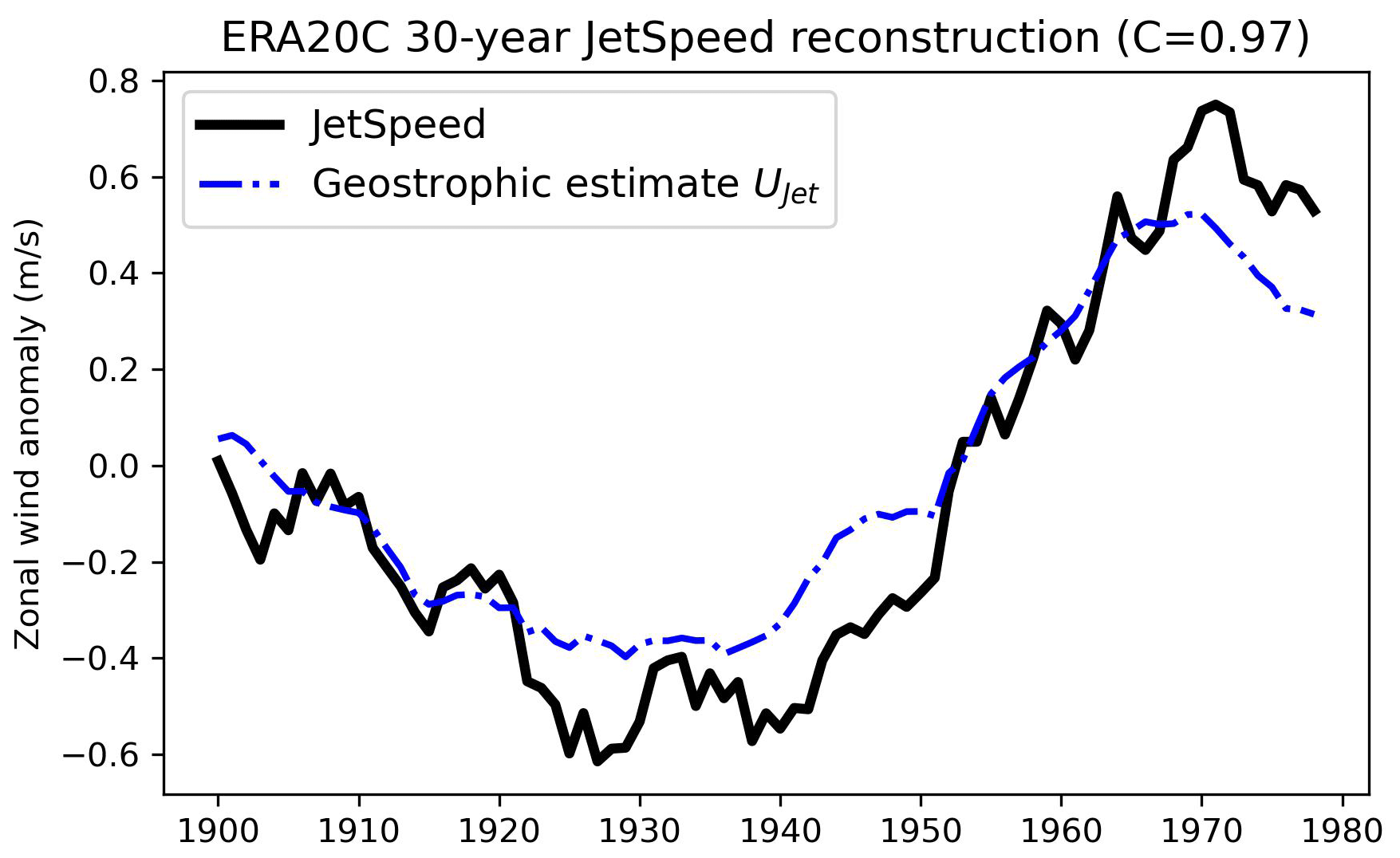
Figure 9 Black curve: 30-year-averaged ERA20C DJF jet speed anomalies. Dashed blue curve: 30-year averages of the ERA20C U_jet anomaly time series, which roughly estimates the anomalous zonal wind variability associated with SPNA-induced changes to the meridional temperature gradient assuming geostrophic balance (see main text for details). The value C denotes the correlation coefficient between the two time series.

We emphasise that the specific nature of the fast-timescale processes responsible for bringing the jet into geostrophic balance, including the role of moist processes, is actively studied (Fuchs et al., 2023; Schemm, 2023), and we do not shed any further light on these. The above analysis simply says that if the SPNA is heating the atmosphere aloft, then geostrophic balance effectively forces the jet speed to exhibit the decadal variability we observe.

Figure 10 Histograms of the SPNA–JetSpeed correlations expected by chance from the seasonal-timescale link (a, d), taking 10-year averages of the seasonal link (b, e), and taking 30-year averages of the seasonal link (c, f). See main text for details. The top row uses data fitted to ASF20C and the bottom to ERA20C. In each subplot the red line indicates the actual correlation found in that dataset, and the dashed lines indicate the 95 % confidence interval. The histograms are normalised so that the area underneath is 1.

5.2 Decadal-timescale forcing as the accumulation of seasonal-timescale forcing

In Sect. 3.2, we argued that the presence of skill in ASF20C implies that predictable jet speed variability is a result of forcing from the boundary conditions taking place already within a single season. Having now argued that this forcing is coming from SPNA SSTs, it remains to be tested whether the forcing exerted by the SPNA on the jet taking place on seasonal timescales suffices to explain the decadal-timescale correlations seen in Table 2. That is, we want to test the following hypothesis: that the jet's response to the SPNA is established within a single season and that the decadal signal seen in the jet speed arises purely from decadal power in the SSTs, without the need to invoke processes or feedbacks on slower, multiannual-to-decadal timescales.

To test this, we model the SPNA–JetSpeed system as follows. For a given dataset, we perform a linear regression of the interannual SPNA time series against the interannual JetSpeed time series to get

$$\begin{array}{}\text{(2)}& \mathrm{JetSpeed}=a\cdot \mathrm{SPNA}+b+\mathit{ϵ}\end{array}$$

for some constants, a and b, and a noise term ϵ, which is normally distributed with mean 0. We then generate a random, synthetic time series of DJF SPNA using the Fourier phase shuffle method, as in the previous subsection. A corresponding JetSpeed time series is then obtained using the linear relationship just derived; the synthetic jet speed thus relies only on the simultaneous synthetic SPNA in that season. We then take 10- and 30-year running means of these synthetic DJF time series and compute the correlations between them. By repeating this procedure 10 000 times we can assess what decadal-timescale correlations are expected from taking running means of the interannual SPNA–JetSpeed link.

The result of this for ASF20C is summarised in Fig. 10a–c. The synthetic seasonal-timescale correlations (Fig. 10a) capture the actual seasonal correlation by construction. After taking running means, the distribution of synthetic correlations becomes notably skewed. For both 10- and 30-year running means (Fig. 10b and c), the observed correlation is still comfortably within the 95 % confidence interval of the synthetic correlations. The same analysis for ERA20C is shown in Fig. 10d–f. The observed 10- and 30-year correlations are closer to the upper threshold here but still fall within it. This implies that the decadal-timescale correlations of ASF20C and ERA20C can be completely explained by the interannual SPNA–JetSpeed link, as hypothesised.

We emphasise that we are not suggesting the SPNA variability is purely interannual but rather that the connection between the SPNA and the atmosphere occurs within the span of a single season. The same conclusion can be seen to hold for CSF20C by comparing Table 2 with Fig. 10; we also verified the analysis using the shorter DPLE (not shown). To further support this point, Fig. 11 shows lag correlations of the jet speed in ERA20C against the SPNA time series (black curve). The correlations peak at lag 0 and diminish towards 0 for increasingly negative lags, consistent with an instantaneous forcing from the (decadally varying) SPNA which slowly diminishes over time. The comparison with the AMV lag correlations (red curve in Fig. 11) will be discussed in Sect. 7.3.

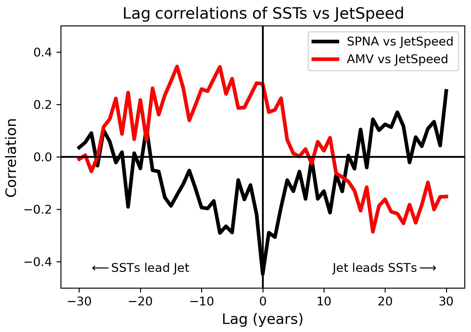
Figure 11 Lag correlations of DJF SPNA (black) and AMV (red) against JetSpeed time series in ERA20C. Negative lags correspond to SSTs leading the jet and positive lags to SSTs lagging the jet. The period covered is 1900–2010.

6 Drivers of decadal SST variability and their link to the jet speed

We have highlighted SSTs in the SPNA as the main source of decadal predictability of the jet speed. Identifying the drivers of SPNA variability and their relation to jet speed variability is thus important for understanding how reliable forecast skill is likely to be in the future. A comprehensive examination of this using the jet speed framework goes beyond the scope of the paper. Here we limit ourselves to only considering two key potential drivers: anthropogenic sulfate aerosols and the AMOC.

6.1 The role of sulfate aerosols

The question of how aerosols affect North Atlantic SSTs is still actively debated and could include the role of both direct radiative adjustments local to the region and more indirect impacts from upstream emissions (Booth et al., 2012; Robson et al., 2022). Here we will only consider the hypothesis put forth by Robson et al. (2022) due to its being based on a large multimodel ensemble, unlike most other studies. In their study, they argued that sulfate aerosol emissions over the eastern part of North America led to a cooling of surface temperatures there and that this cool air was then advected over the North Atlantic, thereby cooling the SSTs and ultimately modulating the AMOC. The possible direct impacts of emissions over the SPNA region itself will not be considered, since the emissions are generally very low in this region.

ERA20C, ASF20C, and CSF20C all share the same prescribed aerosol emissions, namely those used in CMIP5 (Lamarque et al., 2010). The climatological SO₄ emissions are shown in Fig. 12a, showing a clear concentration of emissions over the eastern North American region. To study the impact of these emissions on the SPNA and jet speed, we define an SO₄ time series by averaging the emissions over the box 30–45^∘ N, 100–75^∘ W. This box is visualised in Fig. 12a and approximately covers the eastern North American continent. This time series is compared to the 10-year-averaged SPNA SSTs and ERA20C jet speed in Fig. 12b. The SO₄ time series matches both the SSTs and jet speed in the period 1940–2010, with a correlation of around 0.8. However, in the earlier period 1900–1940, the SO₄ emissions are anticorrelated with the SSTs and jet speed, with a correlation of around −0.3. Note that the CMIP5 aerosol forcing data are constant across each 10-year period, explaining the step-like quality of the SO₄ time series.

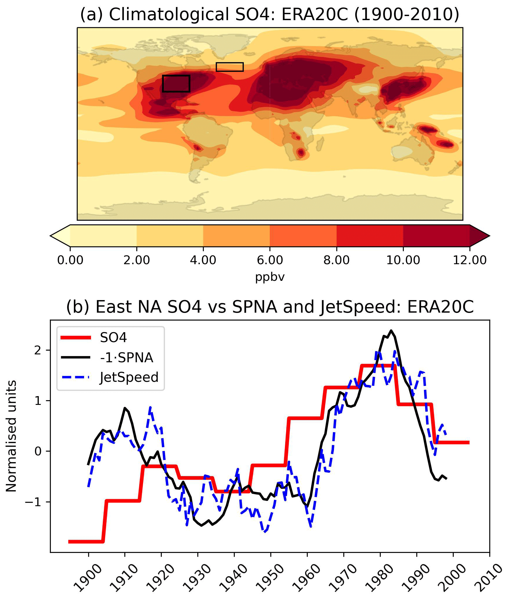
Figure 12 In (a), the climatological SO₄ emissions of ERA20C (in parts per billion by volume), which is the same as those in ASF20C and CSF20C. In (b), time series of the 10-year-averaged ERA20C SPNA SSTs, jet speed and area-averaged eastern North American SO₄. The sign of the SPNA time series has been flipped for visual convenience. In (a), the domain of the eastern North American region has been marked with a thick black box and the SPNA domain with a thin black box.

We conclude that while aerosol emissions over North America may have played a role in driving decadal SPNA variability, they are unlikely to explain the entire 20th century variability, especially in the early period when emissions are still very low. Similar conclusions were drawn in earlier work by Zhang et al. (2013). Note that the forecast models are able to capture the strong jet in this early period despite the low aerosol emissions (Fig. 1). If the aerosols are driving some of the SPNA variability, then this would be expected to lead to predictable shifts in the jet speed, as discussed in the present paper. It should also be noted that an aerosol-induced cooling of North America would strengthen the land–sea contrast, which would also be expected to drive a stronger jet (Portal et al., 2022). It is unclear if such a change in land–sea contrast alone can generate decadal-timescale forecast skill.

6.2 The role of the AMOC

To understand if the AMOC alone can drive SPNA-induced jet speed variability, we examine the two EC-Earth3 pre-industrial control simulations, which we refer to as piControl r₁ and piControl r₂. These simulations are particularly useful for assessing AMOC forcing, since they are known to exhibit large and striking centennial-timescale AMOC oscillations (Meccia et al., 2022). The lack of any anthropogenic emissions means the associated variability in the SPNA will be entirely due to the AMOC.

Figure 13 shows 30-year DJF running means of SPNA SSTs vs. JetSpeed for the two ensemble members. The centennial AMOC oscillations are clearly visible in the SPNA time series. The correlations obtained between the SPNA and JetSpeed are −0.63 for the r₁ member and −0.34 for the r₂ member. A 5 % significance threshold using the same null hypothesis as before (modelling JetSpeed as white noise and SPNA with the Fourier phase shuffle method) is approximately ±0.5, implying that the r₁ correlation is highly significant, while the r₂ is not.

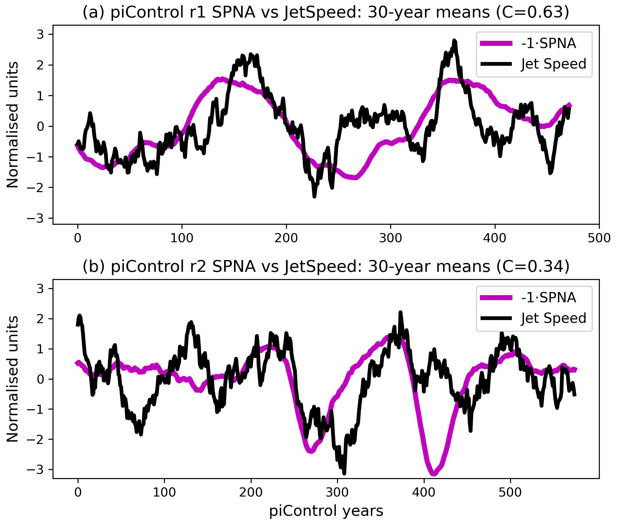
Figure 13 (a) Time series of 30-year averages of the DJF SPNA SSTs (purple) and DJF jet speeds (black) in the first EC-Earth3 pre-industrial control ensemble member. (b) The same for the second ensemble member. The sign of the SPNA time series has been flipped for visual convenience. The value C in the titles indicates the correlation between the two time series. The time series have been normalised to have mean 0 and standard deviation 1.

We cannot directly compare the correlations from these free-running coupled simulations to the ensemble mean correlations of ASF20C. However, we note that if we concatenate five back-to-back ASF20C ensemble members, we get a time series of length $\mathrm{5}\times \mathrm{109}=\mathrm{545}$, approximately the same length as the piControl members. By randomly drawing five ASF20C members, concatenating them, and computing the correlations between the resulting SPNA and JetSpeed time series, we can compare ASF20C and piControl in a like-for-like manner. If we carry out 1000 such random draws, we find that the expected ASF20C correlation is around −0.2 with a 95 % confidence interval of approximately [−0.51, 0.18]. Almost identical results are obtained when using the CSF20C ensemble. This clearly suggests that the r₂ correlation of −0.34 is perfectly consistent with the SPNA–JetSpeed link diagnosed in ASF20C–CSF20C. It also suggests that the r₁ correlation of −0.63 is larger than expected, though not impossible, with a handful of concatenated ASF20C–CSF20C members producing correlations of around −0.6. Since the AMOC oscillations are particularly strong in the piControl runs, it is possible that this translates into SPNA–JetSpeed correlations which may be unrealistically large. The r₁ member may also just be a random outlier.

Based on the above analysis we conclude that AMOC oscillations alone can in principle produce SPNA variations associated with an SPNA–JetSpeed link of the same strength as in the forecast models, even in the absence of any aerosol forcing. It is therefore natural to speculate that the AMOC is responsible for the coherent SPNA and jet speed variability seen in the early 20th century (Fig. 12), and it likely contributes to the variability later on as well.

7 Discussion

7.1 Other potential sources of skill

Our key argument for the importance of the SPNA can be understood as a conditional one: if one assumes that the skill comes from SSTs, then Figs. 3–5 suggest that the SPNA is the responsible region. How reasonable is this assumption? In other words, could the skill originate from somewhere other than the ocean?

It is possible in principle that the skill comes from the stratosphere (Omrani et al., 2014), which has a decorrelation timescale of several months. However, the initial conditions of ASF20C (CSF20C) come from ERA20C (CERA20C), which only assimilates surface variables. Because these do not strongly constrain the stratosphere, the stratospheric variability in ERA20C is highly biased. Indeed, O'Reilly et al. (2019a) found that the amplitude of the quasi-biennial oscillation (QBO) is substantially weaker in ERA20C compared to reanalysis products that assimilate a broader range of atmospheric observations. They also reported a greatly reduced downward propagation in ERA20C. O'Reilly et al. (2019a) also considered the same ASF20C hindcasts and found that the seasonal-timescale association between the QBO and the NAO was essentially zero, unlike in forecasts assimilating the stratosphere. We interpret this as evidence that there is limited scope for skill from stratospheric initial conditions in ASF20C–CSF20C. Another argument towards the stratosphere not driving the predictability was given in Simpson et al. (2018), which showed using reanalysis that the magnitudes of stratospheric anomalies do not match those of the jet on decadal timescales. Note that while they only explicitly discussed March, their Fig. B1 suggest similar conclusions would likely be drawn for DJF.

Besides the stratosphere, the remaining obvious candidates are ice and anthropogenic emissions such as carbon dioxide and aerosols. However, the impact of ice on decadal jet variability has been found to be small compared to SSTs (Peings and Magnusdottir, 2016; Ogawa et al., 2018; Liang et al., 2021). Furthermore, observations of ice are sparse and unevenly distributed prior to 1979, with obvious implications for the potential quality of the ice data used in the ASF20C boundary forcing files. As for anthropogenic emissions, the analysis in Simpson et al. (2018) showed that globally averaged emissions cannot explain the decadal variability in a closely related jet index. This leaves open the possible influence of local emissions. The most obvious way for such local emissions to alter the jet is indirectly by altering the radiative forcing and hence surface temperatures. Such indirect forcings on the jet would manifest themselves as an apparent forcing from surface temperatures. While this could potentially include forcing from temperatures over land, the decorrelation timescale over land is much faster than for SSTs, making a decadal-timescale forcing seem less likely. On the other hand, any indirect forcing via the SSTs would already be visible in Figs. 3 and 4, which highlight the SPNA.

It is hard to exclude the possibility of a more direct impact of aerosols on the jet, e.g. due to an altering of the local radiative fluxes in the troposphere (as opposed to at the surface). Figure 12a shows that sulfate aerosol concentrations are small on the north side of the jet core, making a direct contribution from there seem less likely. There are more emissions centred around the jet core, so these could be playing a role. However, as pointed out in Sect. 6.1, aerosol emissions drop considerably prior to 1940 and become anticorrelated with the jet speed time series in the period 1900–1940 even as forecast skill remains high (Fig. 12b). Such direct effects are therefore unlikely to explain all the observed skill.

While all these other potential sources of skill cannot be conclusively ruled out without targeted forecast experiments, we nevertheless conclude by process of elimination that there is strong evidence towards our assumption that the skill comes from the SSTs and hence from the SPNA in particular.

7.2 The question of causality between ocean and atmosphere

There is an obvious question concerning the causality of the SPNA–JetSpeed link we have proposed, especially since SSTs in the SPNA are known to be particularly sensitive to forcing from the jet (Visbeck et al., 2003; Barrier et al., 2014; Ma et al., 2020). Are the correlations in Table 2 in fact just indicative of stochastic atmospheric forcing on the ocean? Here we discuss several lines of evidence which suggest that at least a considerable portion of the correlations is due to a genuine forcing from the ocean to the atmosphere.

The first key point is the apparent existence of skilful decadal forecasts. We have shown that the SPNA appears to be the only clear, common, SST-based signal between reanalysis and the forecasts we have analysed. If the SPNA–JetSpeed correlations are mostly or entirely reflecting a causal influence of the atmosphere on the ocean, then one seems forced to conclude that the decadal skill does not originate from the SSTs. This is problematic, given the discussion of Sect. 7.1.

Secondly, we remind the reader that ASF20C is uncoupled and uses prescribed boundary forcing, so correlations on interannual timescales in ASF20C cannot arise from a causal influence of the atmosphere on the SSTs in the model. While this is not true for CSF20C and DPLE, which are coupled, the fact that (i) the correlations they attain are entirely comparable to those of ASF20C and (ii) all these correlations are explainable from the interannual link alone (Sect. 5.2) suggests that forcing from the SSTs to the atmosphere constitutes a pragmatic common explanation for the correlations found in all three forecast models. An alternative explanation for the correlations seen in the uncoupled ASF20C would be the existence of a different source of skill, not related to SSTs, which influences both the jet and the SSTs (possibly via the jet). Since the correct SSTs are prescribed to ASF20C, such a common driver could result in correlations of the sort seen in Table 2. However, as before, the hypothetical existence of such a non-SST-related driver is currently unfounded.

Figure 7 shows correlations between DJF SPNA and DJF temperatures and winds. If we rather correlate November SPNA anomalies against DJF temperatures and winds, we get a similar picture, albeit weaker in magnitude, especially for the winds (see Fig. S2). This suggests that the vertical heating is not purely coming from the adjustment of the jet itself but also from processes induced by the SST anomalies. The fact that the heating associated with the SPNA peaks at the surface (Fig. 7a and c) is also suggestive of SST driving. In general, replacing DJF SPNA SSTs with November averages leads to smaller but non-zero correlations of the same sign.

Another important reason for having a high prior for a causal influence from the SPNA is that several studies using idealised models and general circulation models (GCMs) have demonstrated that SST anomalies can causally affect the jet (Palmer and Zhaobo, 1985; Deser et al., 2007; Hassanzadeh and Kuang, 2016; Baker et al., 2017, 2019). Of particular relevance is the recent work of Drews et al. (2023), who carried out pacemaker experiments which suggest that SSTs in the SPNA have a positive impact on decadal forecast skill. We also highlight Baker et al. (2017), who used a dry model to show that imposed heating anomalies modulate the speed of the eddy-driven jet by altering the meridional gradient around the jet core, making the causal pathway we propose here a plausible explanation for the observed decadal forecast skill. An important caveat here is the increasingly recognised role played by moist processes in determining the jet variability, which are not represented in such a dry model (Willison et al., 2013; Papritz and Spengler, 2015; Schemm, 2023; Fuchs et al., 2023). Note, however, that the results of Baker et al. (2017) are generally consistent with those in Baker et al. (2019) using a full moist GCM.

Finally, Simpson et al. (2018) showed that the DPLE forecasts can skilfully predict decadal SPNA SST variability but fail to predict shorter-timescale North Atlantic winds of an appreciable magnitude, strongly suggesting that decadal SPNA variability is not purely driven by stochastic atmospheric forcing. This was further corroborated by Yeager (2020), who found evidence that the SST skill has an abyssal origin. Consistent with this, quantitative estimates of the stochastic forcing in the coupled CSF20C hindcast, using methods such as the one described in Ma et al. (2020), were found to be very small in the SPNA region on decadal timescales, roughly an order of magnitude smaller than the observed SPNA–JetSpeed correlations (not shown).

To conclude, we consider it likely that there is a sufficient causal influence of the SPNA on the jet to explain the observed decadal skill. Unambiguously confirming this would, however, require performing expensive forecast experiments, such as rerunning the full ASF20C hindcast using boundary forcing files from which the SPNA SST variability has been eliminated.

7.3 Relationship with Atlantic Multidecadal Variability

We have argued that the SPNA forces the NAO more or less instantaneously. How do our results relate to previous studies suggesting that the AMV forces the NAO, with the NAO response typically lagging the AMV by several years (Peings and Magnusdottir, 2014b; Peings et al., 2016; Kwon et al., 2020)? We suggest that this apparent discrepancy is a result of three factors.

Firstly, while the AMV pattern on interannual timescales is the famous horseshoe pattern, the pattern largely collapses to a signal confined to the SPNA after performing decadal-timescale smoothing (Delworth et al., 2017; Simpson et al., 2018). This suggests that as far as decadal atmospheric variability is concerned, the SPNA is more relevant than the horseshoe pattern. The importance of this region has been highlighted previously (Gastineau and Frankignoul, 2015; Woollings et al., 2015; Ortega et al., 2017; Delworth et al., 2017; Wills et al., 2019).

Secondly, anomalies in the SPNA (the northern part of the horseshoe) are observed to lead anomalies in the tropical Atlantic (the southern part of the horseshoe) by around 2 years (Zhang, 2007). It is likely that this propagation of anomalies takes place both via subsurface ocean dynamics and coupling with the atmosphere (Zhang et al., 2019). This means that performing analysis based on the standard AMV horseshoe pattern is mixing together different processes happening on different timescales. Since the SPNA anomalies arise first, restricting attention to these might be expected to give a clearer picture and better highlight causal pathways from the ocean to the atmosphere. This argument has also recently been made by Wills et al. (2019). Note that this second point is presumably related to the first, since taking decadal averages would be expected to remove the shorter-timescale signals associated with the propagation of SST anomalies along the horseshoe and processes operating at much slower timescales, such as those associated with deep convection in the Labrador Sea. This argument was also made in Delworth et al. (2017).

Thirdly, the reverse impact of the NAO on the AMV has also been noted to operate on both fast and slow multiyear timescales (Ma et al., 2020; Khatri et al., 2022), introducing additional lags to the coupled AMV–NAO system.

We therefore suggest that the apparent existence of an NAO response lagging the AMV by several years is, in fact, largely reflecting the existence of an essentially instantaneous atmospheric response to the SPNA, with the multiyear lag being an artefact of using an AMV index which averages across several different processes. This is further supported by Fig. 11. The AMV–JetSpeed lag correlations (red curve) show a peak at 7–15 years (depending on smoothing choices) when the AMV leads, reproducing what is found using the NAO index (Peings and Magnusdottir, 2014b; Peings et al., 2016). When the SPNA index is used, this lag vanishes, with correlations now peaking at lag 0.

7.4 Why is the jet latitude not predictable?

Several studies have argued that an AMV-driven NAO response involves a shift in both the strength and location of the storm track and/or baroclinic region (Msadek et al., 2011; Peings and Magnusdottir, 2014a; Frankignoul et al., 2015; Peings et al., 2016; Ortega et al., 2017). Such systematic latitudinal shifts in the storm track and/or baroclinicity, and hence the eddies, would be expected to manifest as predictable latitudinal shifts in the eddy-driven jet itself. However, as discussed in Sect. 3, there is no decadal predictability of the latitude of the jet in ASF20C, CSF20C, or DPLE. This suggests that on decadal timescales the eddies are randomly distributed around their mean position and that the mechanism driving predictable jet variability does not essentially depend on latitudinal shifts in the storm track. Rather, such predictable changes appear to be more clearly related to the direct constraint of thermal wind balance along with an intensification of the storm track. This is fully consistent with Woollings et al. (2015), who highlighted the contrasting nature of forced shifts to the latitude and speed of the jet.

Of course, it cannot be ruled out that SST anomalies in the SPNA, or indeed elsewhere, force shifts in the latitude of the jet in the real world that are simply not captured by the forecast models we considered. However, until predictability has been established it does not seem possible to reject the null hypothesis that decadal variability in the jet latitude is chaotic and unpredictable. Indeed, the inconsistent latitudinal response in multimodel studies such as Ruggieri et al. (2021) lends concrete evidence for such inherent chaos. Further evidence for this is given in Fig. S3, which repeats the procedure of Sect. 4 to search for potential sources of jet latitude skill in ASF20C. This shows that there are no regions of significant SST–jet latitude correlations common to both ERA20C and ASF20C, consistent with the lack of jet latitude predictability.

It is also possible that biases in the climatological jet latitude (i.e. in the model mean state) of the forecast models are contributing to the apparent lack of jet latitude predictability. The sensitivity analysis of Baker et al. (2017) showed that the response of the jet latitude to thermal forcing changes sign abruptly around the jet core, while the response of the jet speed is more uniform across the jet. The accurate response of a model jet to a given SST anomaly may therefore differ dramatically based on its climatological position. This could go some way to explaining the inconsistent jet latitude response in multimodel studies such as Ruggieri et al. (2021).

8 Conclusions

We briefly summarise the main results and arguments.

1. The decadal forecast skill of the winter NAO appears to be entirely due to the decadal predictability of the speed of the North Atlantic jet. There is no apparent predictability of decadal variations in the latitude of the jet, even in seasonal hindcasts with prescribed SSTs (Figs. 1 and 2).

2. Initialised seasonal hindcasts can skilfully reproduce decadal variations in jet speed all the way back to 1900 and match the behaviour of a genuine decadal forecast in the period 1954–2010. This justifies using such seasonal hindcasts to diagnose decadal forecast signals using the full period 1900–2010, effectively doubling the available years compared to existing decadal forecasts. In addition, this strongly suggests that the decadal forecast signals are already fully present and visible on interannual timescales.

3. The only clear source of an interannual-to-decadal jet speed signal coming from SSTs, common to reanalysis and forecasts, is the SPNA region (Figs. 3 and 4). SSTs in this region enjoy large and statistically significant correlations with the jet speed, which we argue are due at least in part to a causal link from the ocean to the atmosphere (Fig. 6). We also show that all of the decadal SPNA–JetSpeed links in the forecast models, along with the associated forecast skill, can be explained by a small but consistent seasonal-timescale forcing from the SSTs (Figs. 10 and 11).

4. The pathway from SPNA SSTs to the jet speed is argued to be tropospheric in nature: the surface heating anomaly extends relatively deeply into the troposphere (Fig. 7) and is optimally situated to perturb the jet speed both by direct adjustments consistent with thermal wind balance and subsequent reinforcements by the eddies.

5. Sulfate aerosol emissions in North America may explain part of the 20th century covariability in the SPNA and jet speed but do not explain the early 20th century (Fig. 12). AMOC oscillations alone are shown to be capable of inducing SST shifts in strength comparable to those connected with jet speed variability (Fig. 13).

Note that the importance of the SPNA in driving predictable decadal jet variability was emphasised in Simpson et al. (2018) using a different metric of North Atlantic jet variability in March. Our work here is clearly closely related to and was directly inspired by theirs.

There are several shortcomings to our analysis, chief of which is the fact that we have only studied two independent forecast models. However, Marcheggiani et al. (2023) have recently analysed the decadal forecasts used in Smith et al. (2019) and found that the jet speed is much more predictable than the jet latitude. They also linked the predictability to North Atlantic SSTs, thereby reinforcing two of our key conclusions using independent data. Our argument that the stratosphere is unlikely to be relevant due to the initialisation biases of the seasonal hindcasts may also be flawed, and it would be of interest to examine the role of the stratosphere more closely. We also interpreted the similar jet speed correlations in ASF20C–CSF20C and DPLE as evidence that the mechanisms involved are the same for these datasets. However, it may be that ASF20C–CSF20C obtain most of their “skill” from the initialisation (lag 0), while DPLE obtains most of its skill from representing slower-frequency coupled processes better (lags > 0). If so, conclusions drawn using ASF20C–CSF20C may not carry over to a genuine forecast context. Nevertheless, our findings have some important implications.

To begin with, we have reinforced the conclusion of earlier studies such as Baker et al. (2017), which is that the speed and latitude of the jet should be considered separately and that the use of indices like the NAO (which amalgamate the two) may be misleading. Our finding that the decadally averaged jet speed is predictable while the latitude is not stands in amusing contrast to work on seasonal forecasts, which suggest the opposite picture of a predictable latitude and unpredictable speed (Parker et al., 2019). This reinforces the analysis of Woollings et al. (2015), who showed that the nature of forced jet variability differs depending on the timescale. On interannual timescales, the variability is dominated by the jet latitude, in turn associated with meridional shifts in the transient eddies and location of blocking. On decadal timescales, the variability is dominated by the jet speed, in turn associated with changes both to the strength of the eddy forcing and to the occurrence of transient Rossby wave breaking on both sides of the jet. Our analysis corroborates the speculation in Woollings et al. (2015) that this may result in the nature and sources of predictability being different on the two timescales. In particular, our results are consistent with the following hypothetical view of the jet variability:

• a.

  On seasonal timescales the forcing from the SPNA is too small to be easily visible (resulting in the appearance of no jet speed skill), with jet latitude skill arising from accurately predicting meridional shifts in the eddies.

• b.

  On decadal timescales the eddies are varying essentially chaotically around their climatological position (resulting in no jet latitude predictability), but their intensity can vary predictably depending on the underlying SPNA SSTs, which strengthen or weaken the meridional temperature gradient.

A novelty of our work is the use of the initialised 20th century seasonal hindcast products ASF20C and CSF20C. While Parker et al. (2019) considered the fast and slow variability in the jet speed and latitude in ASF20C, the possibility of utilising these hindcasts to study the mechanisms underpinning decadal predictability seems to have been overlooked. Properties of ASF20C, i.e. covering the entire 20th century, being re-initialised every year, and being uncoupled, are all highly attractive for simplifying analysis which we made extensive use of. We believe that ASF20C may be similarly beneficial for the study of decadal predictability in many other contexts.

Finally, we add to a growing body of literature suggesting that the SPNA is the main source of North Atlantic jet forcing on decadal timescales and that the use of a larger AMV or AMOC pattern might be counterproductive for questions of predictability by mixing together different mechanisms and timescales. We have shown that the SST variability in the SPNA driving predictable jet speed shifts can in principle be due to both the AMOC and aerosol emissions, and it seems likely that the observed 20th century variability is a result of both of these. We do not shed further light in this study on the signal-to-noise paradox, but our results suggest that it may be particularly interesting to examine how well forecast models simulate fast-timescale atmosphere–ocean coupling in the SPNA region. This is a natural avenue for future work.