Waviness of the Southern Hemisphere wintertime polar and subtropical jets

The recently developed average latitudinal displacement (ALD) methodology is applied to assess the waviness of the austral-winter subtropical and polar jets using three different reanalysis data sets. As in the wintertime Northern Hemisphere, both jets in the Southern Hemisphere have become systematically wavier over the time series and the waviness of each jet evolves quite independently of the other during most cold seasons. Also, like its Northern Hemisphere equivalent, the Southern Hemisphere polar jet exhibits no trend in speed (though it is notably slower), while its poleward shift is statistically significant. In contrast to its Northern Hemisphere counterpart, the austral subtropical jet has undergone both a systematic increase in speed and a statistically significant poleward migration. Composite differences between the waviest and least wavy seasons for each species suggest that the Southern Hemisphere's lower-stratospheric polar vortex is negatively impacted by unusually wavy tropopause-level jets of either species. These results are considered in the context of trends in the Southern Annular Mode as well as the findings of other related studies.

1 Introduction

Consideration of changes in the behavior of the tropopause-level jet streams in a warming world has been catalyzed by the construction of long-period reanalysis data sets over the past 3 decades (Kalnay et al., 1996; Kistler et al., 2001; Kobayashi et al., 2015; Copernicus Climate Change Services (CS3), 2017). Recent analyses employing these data sets (e.g., Archer and Caldeira, 2008; Barnes and Screen, 2015; Gallego et al., 2005; Manney and Hegglin, 2018; Peña-Ortiz et al., 2013; Vavrus et al., 2017), in tandem with a number of studies based upon climate model output (e.g., Barnes and Polvani, 2013; Lorenz and DeWeaver, 2007; Miller et al., 2006; Yin, 2005), have produced a consensus view that poleward displacement of both jets accompanies warming. Along with an interest in latitudinal position, nearly all of the aforementioned studies have also addressed observed and/or forecasted changes in the speed of the jet streams.

In a recent paper Martin (2021) offered a feature-based analysis of the waviness of the tropopause-level polar and subtropical jets during Northern Hemisphere (NH) winter (DJF, December–January–February). The analysis proceeded from the results of Christenson et al. (2017) that identified the isentropic layers that house the two species of jets during NH winter. They found that (1) the polar jet (POLJ) has undergone a statistically significant poleward migration over the time series, not matched by the subtropical jet (STJ), and (2) neither jet species exhibited a trend in its speed. Additionally, the analysis showed that both jets have become systematically wavier over the last 6 decades.

By virtue of its land–sea distribution, enhanced lower-tropospheric warming at high latitudes of the NH, known as Arctic amplification, has recently emerged as a prominent signal of climate change (e.g., Serreze et al., 2009; Screen and Simmonds, 2013: and references therein). Francis and Vavrus (2012) were among the first to propose that changes in the undulatory nature of the jet stream might be linked to Arctic amplification. This suggestion initiated a decade-long debate on this issue (e.g., Barnes, 2013; Blackport and Screen, 2020; DiCapua and Coumou, 2016; Francis, 2017; Francis and Vavrus, 2015; Francis et al., 2018; Martineau et al., 2017; Screen and Simmonds, 2013; Vavrus, 2018). As noted by Martin (2021), at least some of the controversy and attendant lack of consensus surrounding this question (Barnes and Polvani, 2015) was nourished by the absence of a robust method of assessing the waviness of the tropopause-level jets. The average latitudinal displacement (ALD) methodology introduced in Martin (2021) (briefly described later) offers one possible remedy for this deficiency.

The principal mode of variability in the Southern Hemisphere (SH) extratropical circulation is the Southern Annular Mode (SAM; Limpasuvan and Hartmann, 1999; Gong and Wang, 1999; Thompson and Wallace, 2000), a nearly zonally symmetric structure with coincident geopotential height anomalies of opposite signs in Antarctica and the middle latitudes. In the decades prior to 2000, the SH jets shifted poleward and the SAM has tended toward positive polarity (e.g., Fogt and Marshall, 2020). These coincident trends have been presumed to be a result of ozone depletion. As the ozone recovers in the SH, simulations suggest a reversal of this trend may be forthcoming (WMO, 2022). Spensberger et al. (2020) have questioned whether the associated jet displacement also explains shifts in the storm tracks across the hemisphere. Instead they suggest that the SAM can be interpreted as a measure of the degree of coupling (or decoupling) between Antarctica and the southern mid-latitudes.

Recently, considerable attention has been devoted to interrogating the zonally asymmetric component of the SAM (e.g., Fan, 2007; Silvestri and Vera, 2009; Fogt et al., 2012; Rosso et al., 2018; Campitelli et al., 2022). This asymmetric component is characterized by a wave-3 pattern (Goyal et al., 2021; Goyal and England, 2022; Campitelli et al., 2022) with a maximum amplitude at 250 hPa in the Pacific and may be determinative of the overall positive trend in the SAM over the reanalysis era. Such a wave-3, tropopause-level signal is immediately suggestive of the influence of the jets. These observations motivate consideration of the direct measurement of the waviness of the SH wintertime jets.

Despite a number of recent studies that consider aspects of the interannual variability of the austral-winter subtropical jet (e.g., Gillett et al., 2021; Maher et al., 2020), to our knowledge, a study by Gallego et al. (2005) is the only one to consider direct measurement of the waviness of the austral-winter jets. They employed an objective method focused on identifying the geostrophic streamline of maximum average velocity at 200 hPa (i.e., the jet core at that level) to separately consider the behaviors of the STJ and POLJ. This method allowed for the consideration of the jets as continuous features around the hemisphere and thus enabled a number of novel analyses of their behavior and trends. With particular relevance to the present study, they considered a zonal index computed as the difference between the maximum and minimum latitude of the jet core (i.e., the streamline at the core of the jet) on each day. A similar metric, termed DayMaxMin, was employed by Barnes (2013) in her consideration of the behavior of the NH 500 hPa flow. Though insightful, such a metric does not comprehensively account for the waviness created by the full collection of troughs and ridges around the hemisphere that routinely characterizes the jets.

In this paper we apply the methodology of Martin (2021) to assess recent trends in the waviness of the SH wintertime polar and subtropical jets. The method of identifying the austral-winter polar and subtropical jet locations in isentropic space is described in Sect. 2 along with a description of the data sets used. Also included there is a short description of the method of assessing waviness introduced in Martin (2021). In Sect. 3, elements of the long-term trend and interannual variability of the waviness of the austral-winter polar and subtropical jets are presented along with differences between composites of the waviest and least wavy seasons for each species. A summary and conclusions are offered in Sect. 4.

2 Data and methodology

In the foregoing analysis, the zonal (u) and meridional (v) winds as well as temperature (T) at 6 h intervals from three different reanalysis data sets are employed. A total of 72 austral winters (JJA, June–July–August) (1948–2019) of the NCEP/NCAR (National Centers for Environmental Prediction/National Center for Atmospheric Research) Reanalysis at 17 isobaric levels at 10 hPa on a 2.5^∘ latitude–longitude grid (Kalnay et al., 1996; Kistler et al., 2001) are used. We employ 62 winters (1958–2019) of the Japanese 55-year Reanalysis (JRA-55) with data on 60 vertical levels up to 0.1 hPa on a horizontal grid mesh of ∼ 55 km (Kobayashi et al., 2015). Finally, the ERA5 reanalysis data set on 137 vertical levels from the surface to 80 km with a grid spacing of 31 km covering the period from 1979 to 2019 (Copernicus Climate Change Service (CS3), 2017) are used as well. The waviness of the jets is assessed in the context of understanding their relationships to the horizontal gradient of potential vorticity (PV) in prescribed isentropic layers. A similar approach was taken with respect to the STJ in recent work by Maher et al. (2020). The first step in the present analysis involves identification of the isentropic layers that house the austral-winter jets. This was accomplished empirically by identifying the isentropic level at which the maximum wind speed was observed in each grid column (between 10 and 80^∘ S) at each analysis time in JJA over the 62-year time series of the JRA-55 data set. The use of isentropic space here differs from the insightful approach taken by Manney et al. (2017) and Manney and Hegglin (2018) which employed separate latitude and elevation criteria to differentiate between the STJ and the POLJ. Of the three data sets employed in the present work, the JRA-55 was chosen for this preliminary analysis step because both its length of the time series and its horizontal and vertical resolutions are between those characterizing the other two data sets employed here. Following Koch et al. (2006) we only considered columns in which the integral average wind speed exceeded 30 m s⁻¹ in the 100–400 hPa layer. The resulting distribution is clearly trimodal with frequency maxima, and therefore separate jet features, approximately located in the 305–320, 340–355, and 395–410 K isentropic layers (Fig. 1a). The latter isentropic layer appears in the lower stratosphere and is associated with the austral polar night jet (PNJ), which, being located above the tropopause, is not a focus of the present analysis. Further separation of the STJ and POLJ is achieved through a reference to Fig. 2 of Gallego et al. (2005) which strongly implies that the STJ sharply peaks near 30^∘ S, while the POLJ more broadly peaks around 50^∘ S. Accordingly, we further constrained the analysis to latitude bins 0–40^∘ S for the STJ and 40–65^∘ S for the POLJ. With this additional refinement, the analysis identifies the STJ in the 340–355 K isentropic layer and the POLJ in the 310–325 K isentropic layer (Fig. 1b). Similar analyses of the other two data sets (not shown) revealed the robustness of this result. It is important to note that 53.8 % of all qualifying columns (to 380 K) in the 0–40^∘ S bin (STJ) were in the 340–355 K layer, while 46.8 % of all qualifying columns in the 40–65^∘ S bin (POLJ) were in the 310–325 K layer supporting the isentropic assignments for the two species mentioned previously. It is immediately apparent, consistent with prior analyses (e.g., Bals-Elsholz et al., 2001; Nakamura and Shimpo 2004; Gallego et al., 2005), that the STJ is the dominant jet feature in the southern winter.

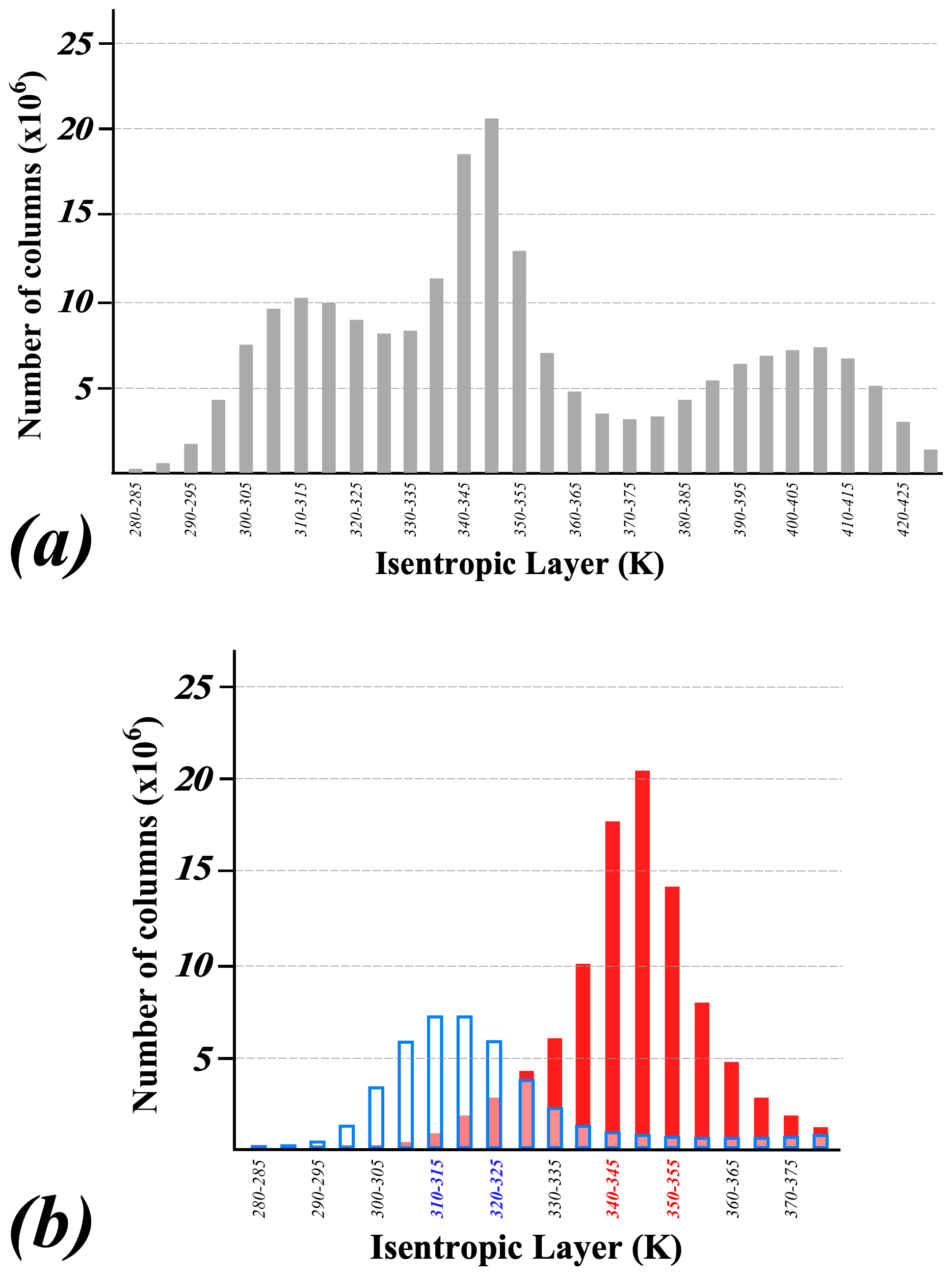
Figure 1 (a) Distribution of grid column maximum wind speeds found in 5 K isentropic layers from 10–80^∘ S for every 6 h analysis time period in JJA from 1958–2019 from the JRA-55 reanalysis. (b) As for Fig. 1a except limited to (i) grid columns in which the integral average wind speed from 400 to 100 hPa exceeded 30 m s⁻¹ and (ii) latitudes at 0–40^∘ S for the STJ or (iii) latitudes at 40–65^∘ S for the POLJ.

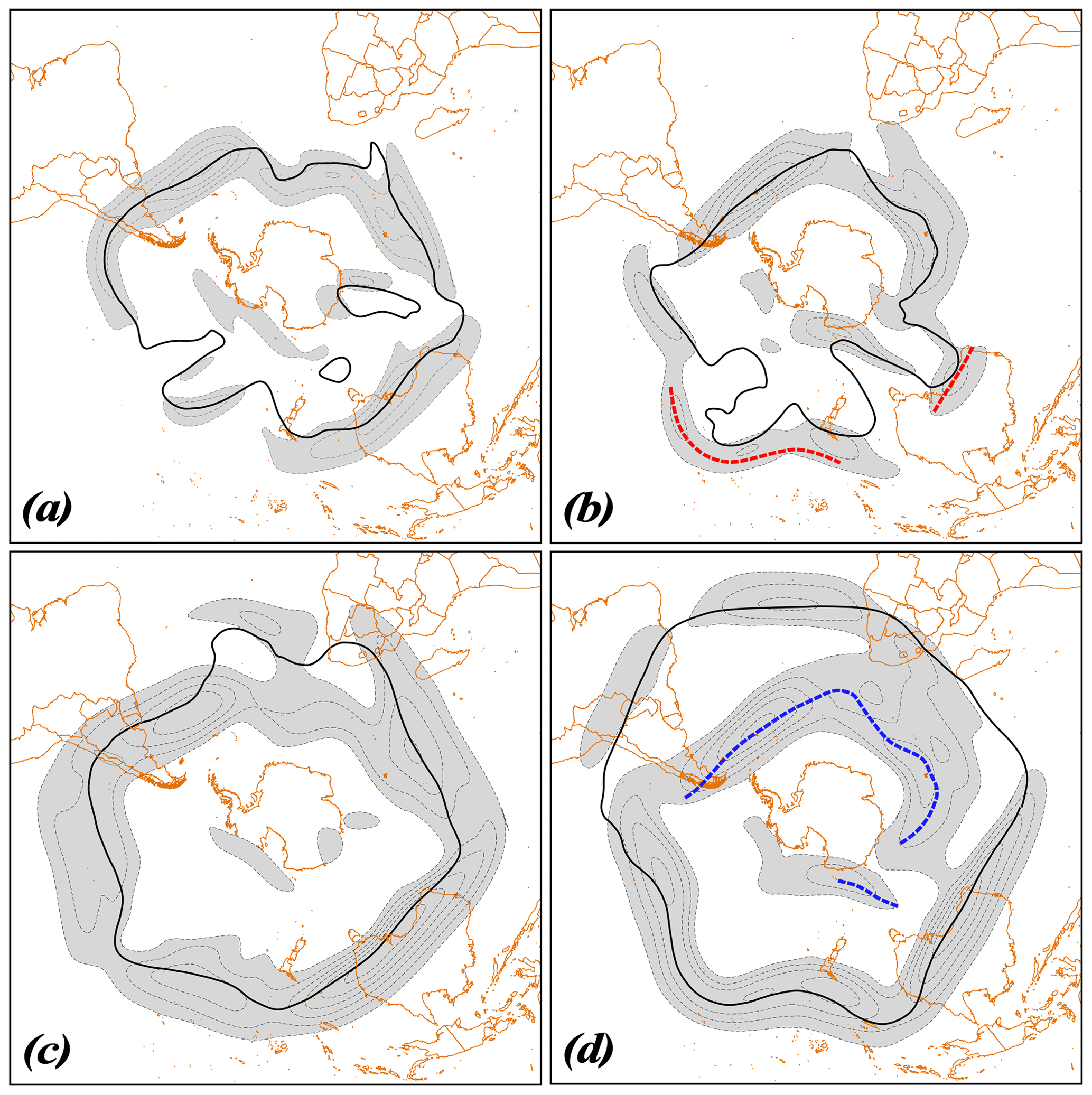
Figure 2 (a) Isotachs of the daily averaged wind speed (contoured every 10 m s⁻¹ and shaded above 30 m s⁻¹) and the core isertel (bold black line) in the 310 : 325 K isentropic layer on 13 July 1995 from the JRA-55 reanalysis data. The core isertel value is −1.3 PVU. (b) As in (a) but for 24 August 2001. Core isertel value is −2.0 PVU. Dashed red line indicates a portion of the core isertel from the overlying STJ layer (depicted in Fig. 2d). (c) As in (a) but for wind speeds and the core isertel in the 340 : 355 K isentropic layer on 13 July 1995. Core isertel value is −3.6 PVU. (d) As in (c) but for 24 August 2001. Core isertel value is −1.4 PVU. Dashed blue line indicates a portion of the core isertel from the underlying POLJ layer (depicted in Fig. 2b). See the text for further explanation.

The analysis method to be used here involves assessment of the circulation which requires calculation of the contour length. As a result, a fair comparison among the different data sets requires adoption of a uniform grid spacing. Consequently, all three data sets were bilinearly interpolated onto isentropic surfaces at 5 K intervals (from 280 to 380 K) and 2.5^∘ latitude–longitude grid spacing using programs within the General Meteorological Analysis Package (GEMPAK) (desJardins et al., 1991). The daily average PV and daily average zonal and meridional wind speeds in both the polar-jet (310 : 325 K) and subtropical-jet (340 : 355 K) layers were then calculated from the data taken four times each day in each of the three time series.

As reviewed in Martin (2021), consideration of the quasi-geostrophic potential vorticity (QGPV), following Cunningham and Keyser (2004), demonstrates that local maxima in the cross-flow gradient of QGPV are collocated with maxima in the geostrophic wind speed. In the Southern Hemisphere, the jets lie on the high-PV edge of this PV gradient. By searching through daily average isertels from −0.5 to −5.0 at 0.1 PVU intervals (1 PVU = 10⁻⁶ m² K kg⁻¹ s⁻¹), the analysis identifies a “core isertel” along which the circulation per unit length (i.e., average speed) is maximized in the separate POLJ (310 : 325 K) and STJ (340 : 355 K) isentropic layers for every day in each of the time series. This core isertel is, by design, an analytical proxy for the jet core. A glimpse into the fidelity of this method in identifying the meandering cores of the POLJ and STJ jets is illustrated in Fig. 2. In each case the objectively identified core isertel, in black, lies very near, or at, the center of the analyzed isotach maxima around the hemisphere with physically defensible exceptions. For instance, the dashed red lines in Fig. 2b indicate portions of the bold black line in Fig. 2d (i.e., the overlying STJ core), suggesting that those portions of the isotach maxima in Fig. 2b that are somewhat removed from the POLJ core isertel are the lower portions of the overlying STJ core. Similarly, an extensive isotach maxima region in Fig. 2d has a dashed blue line, a portion of the bold black line in Fig. 2b, slicing through it. This region, well poleward of the STJ core isertel, is clearly the upper portion of the underlying POLJ core.

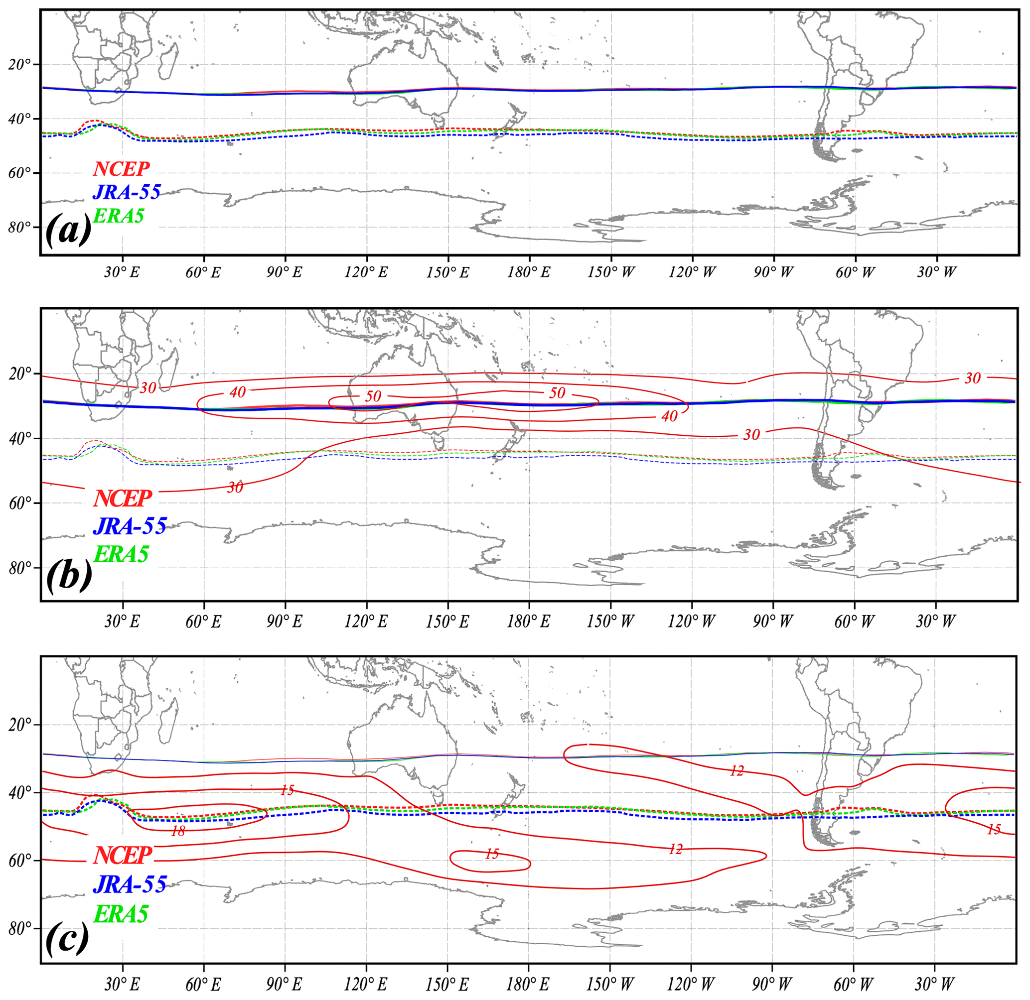
Figure 3 (a) Solid (dashed) lines are the positions of the average core isertels of the STJ (POLJ) from each of the three reanalyses employed in this study. The different reanalyses are color coded. (b) Thick solid lines are the positions of the average core isertels for the STJ from each of the reanalyses superimposed with JJA-average 200 hPa isotachs from the NCEP/NCAR Reanalysis. (c) Thick dashed lines are the positions of the average core isertels for the POLJ superimposed with JJA-average 700 hPa isotachs from the NCEP/NCAR Reanalysis.

Figure 3a shows the average latitude for the core isertels of each jet species from each of the three reanalyses data sets used in the study. The analyses return essentially identical results for the core isertel of the STJ and very nearly identical results for the POLJ. Superimposing the NCEP/NCAR Reanalysis' JJA-average 200 hPa isotachs on top of the STJ core isertels (Fig. 3b) illustrates the fact that the average core isertel accurately represents the axis of the average STJ. The relationship is also strong between the POLJ core isertels and the 700 hPa average isotachs (Fig. 3c).

The waviness of each jet is assessed by calculating a hemispheric average of the meridional displacements of the core isertel from its equivalent latitude – the northern extent of a polar cap whose area is equal to the area enclosed by the core isertel. This metric is referred to as the average latitudinal displacement (ALD). The method requires the core isertel to be the same neither in both jet layers on a given day nor from day to day in a given jet layer. Consequently, it is important to examine its distribution in each jet layer over the entire time series. Figure 4 portrays the frequency of the occurrence of the core isertels in both the STJ and POLJ layers for each of the three time series. The STJ core isertels peak between −1.95 and −2.1 PVU across the three data sets. Considering all three data sets, 81.5 % of all JJA days exhibit a core isertel between −1 and −3 PVU in the STJ layer. The POLJ distribution is shifted toward higher PV values. Overall, 74.8 % of JJA days had a core isertel between −1 and −3 PVU in the POLJ layer. The frequency of occurrence in the several isertelic bins for each species of the SH jet match quite well with what Martin (2021) found for the NH wintertime jets, even when accommodating for the different isentropic layer for the austral POLJ.

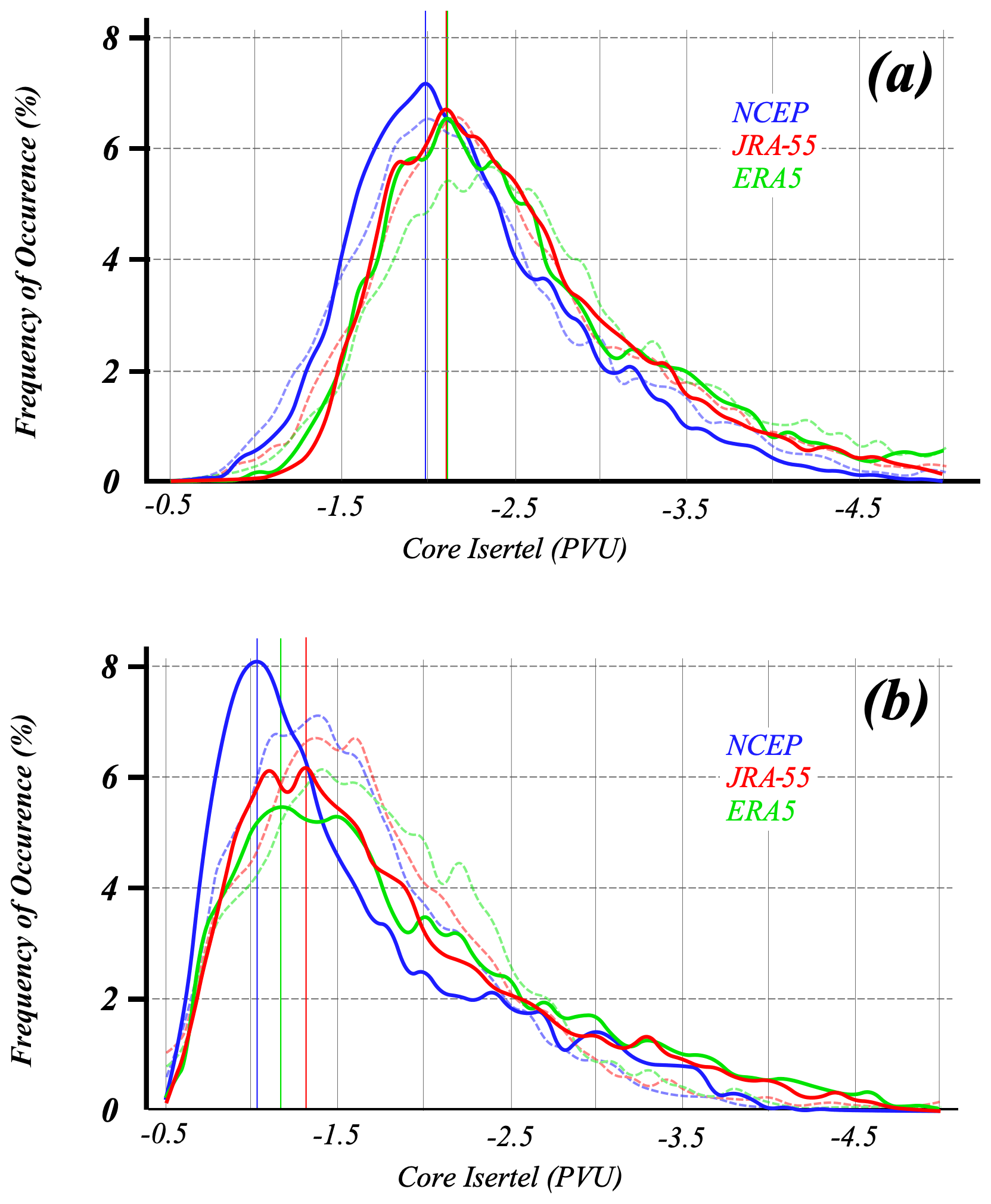
Figure 4 Frequency of the occurrence of the core isertel value for each reanalysis time series in (a) the STJ layer and (b) the POLJ layer. Solid blue, red, and green lines in (a) and (b) are the SH distributions from the NCEP/NCAR, JRA-55, and ERA5 reanalyses, respectively. The dashed blue, red, and green lines are the NH distributions from the NCEP/NCAR, JRA-55, and ERA5 reanalyses, respectively. In (b), the NH distributions are from the 315 : 330 K layer, which houses the POLJ in the boreal winter. Thin blue, red, and green lines in (a) and (b) indicate the peak values of the core isertel in each layer from each data set. Isertel values are given in potential vorticity units (PVU, 1 PVU = 10⁶ K m² kg⁻¹ s⁻¹) and are multiplied by −1 for the NH values.

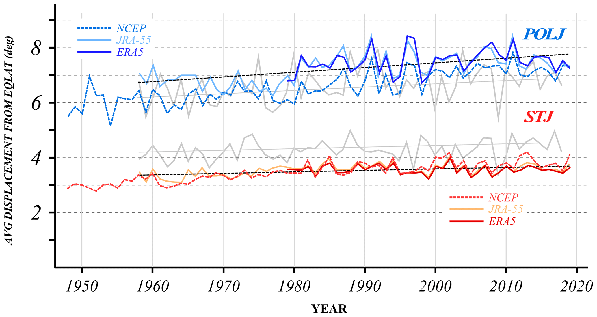
Figure 5 Seasonal-average ALD (in degrees) of the SH wintertime subtropical and polar jets for each cold season in the three reanalysis time series. The polar jet values are in the three shades of blue, while the subtropical jet values are in the three shades of red. The dashed black line through each time series represents the trend line for each (derived from the JRA-55 time series) and is significant at the 96 % level. Gray lines are the boreal-winter ALD analysis from Fig. 6 of Martin (2021). The year on the x axis indicates the year in which December of that cold season occurred. EQLAT: equivalent latitude.

3 Analysis

The JJA-average latitudinal displacement (ALD) of each jet is calculated as a 92 d average of the daily ALD in each cold season. The results are shown in Fig. 5. It is instantly clear that, as in the NH, the POLJ is wavier than the STJ and that both jets have become systematically wavier over the 62-year JRA-55 time series with p < 0.004 for both time series (a one-sided Student's t test was employed). Interestingly, the austral-winter STJ is less wavy than its NH counterpart, but the waviness of both has increased identically at 0.005^∘ yr⁻¹ (0.0125^∘ yr⁻¹ for NCEP/NCAR since 1958 and −0.001^∘ yr⁻¹ for ERA5). The winter POLJ in the SH is, on the other hand, wavier than in the NH and is trending faster (0.017 versus 0.009^∘ yr⁻¹; 0.023^∘ yr⁻¹ for NCEP/NCAR since 1958 and 0.009^∘ yr⁻¹ for ERA5) than its NH complement. Daily time series of the ALD of each jet can also be examined to determine the extent to which the waviness of the two jets covaries. Figure 6 illustrates the POLJ and STJ daily ALDs for 1999 from each of the three data sets. The low correlation between the waviness of the two species in this example year represents the rule rather than the exception. All told, more than 93 % of the STJ and POLJ ALD seasonal time series constructed for this study are correlated with magnitudes less than 0.3. This result strongly suggests that the waviness of the two species evolves independently.

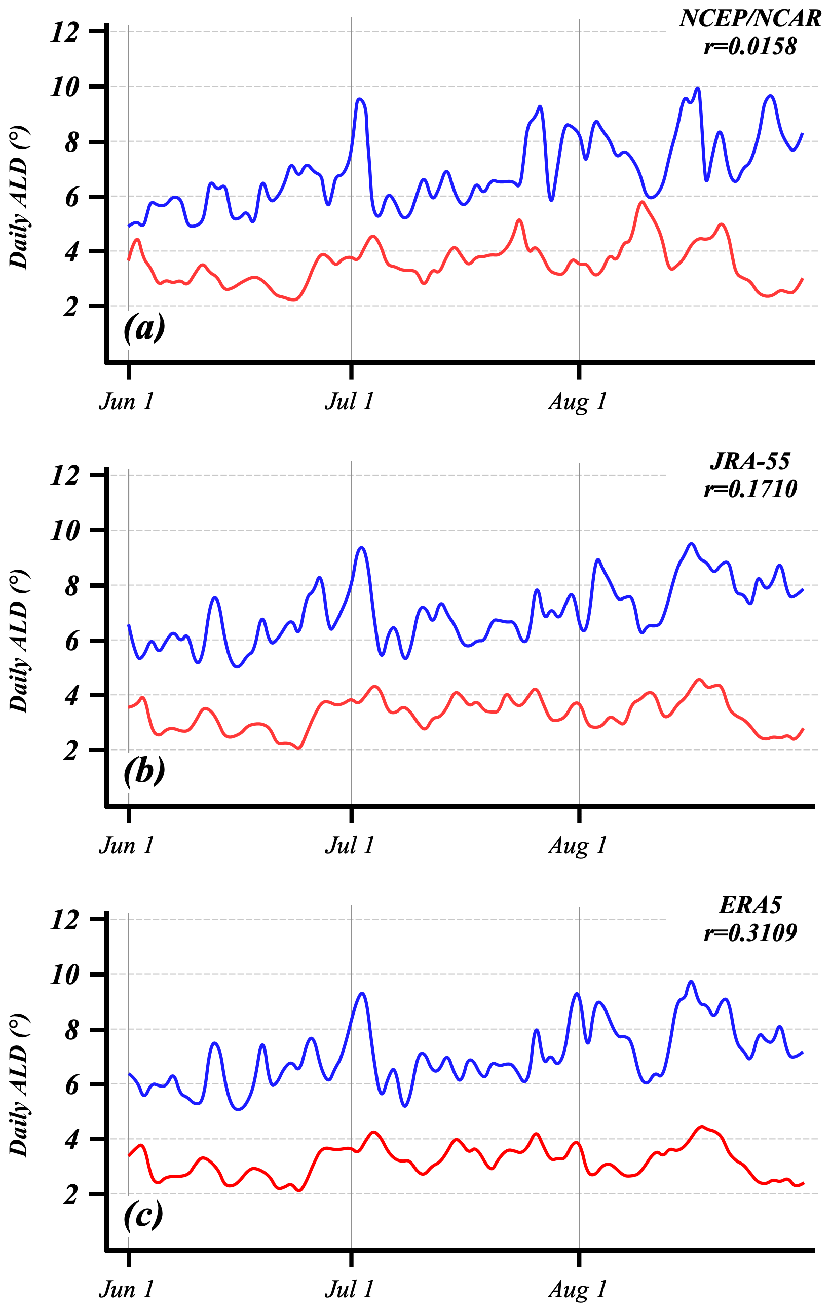
Figure 6 Time series of the daily ALD of the polar (blue lines) and subtropical (red lines) jets from the (a) NCEP/NCAR Reanalysis, (b) JRA-55, and (c) ERA5 data sets for austral winter 1999. The correlation between the two times series from each data set is indicated.

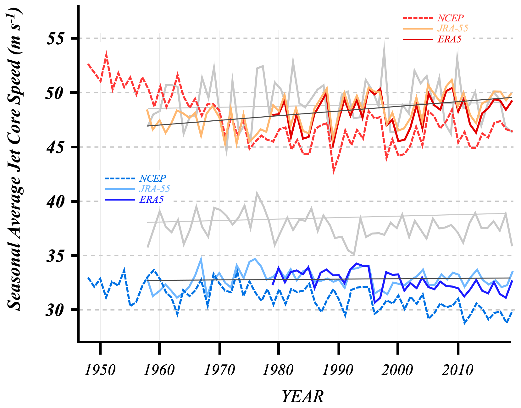
Figure 7 Seasonal-average U along the core isertel for the subtropical (red lines) and polar (blue lines) jets from each of the three SH reanalysis data sets. The thin black lines are trend lines for each time series from the JRA-55 data. Gray lines are the equivalent boreal-winter U analysis from Fig. 9 of Martin (2021).

By definition, the average wind speed along the chosen core isertel on any given day represents the average jet speed for that species on that day. Time series of seasonal-average jet core wind speeds for the wintertime STJ and POLJ in both hemispheres are shown in Fig. 7. As in the NH winter (Martin, 2021), the austral POLJ shows almost no trend in jet core speed and the slight change is not statistically significant. Notably, however, the SH POLJ is ∼ 6 m s⁻¹ slower on average than its NH equivalent. Aside from the fact that the NCEP/NCAR Reanalysis is quite different from the JRA-55 until about 1970, the austral-winter STJ exhibits a robust, as well as statistically significant (p value < 0.001), increase in speed over the JRA-55 time series – in clear contrast to its NH counterpart. It is also apparent that the SH STJ is slightly weaker but less interannually variable than the NH STJ.

Another characteristic of interest that emerges directly from the ALD analysis method is the daily value of the jet core's equivalent latitude which closely approximates its zonally averaged position. Consequently, it is straightforward to construct a time series of the seasonal-average equivalent latitudes of the two species of jets, shown in Fig. 8. Again, as in the NH, the poleward shift of the SH POLJ is occurring 3 times faster than that exhibited by the STJ. In contrast to the situation in the NH, however, the slight poleward displacement of the SH STJ is, like that of the POLJ, statistically significant (p values for the POLJ and STJ are < 0.001 and 0.002, respectively). It is interesting to note that while the SH STJ is located at a latitude roughly similar to the NH STJ throughout the time series, the SH POLJ is ∼ 4^∘ further poleward during winter than the NH POLJ. Overall, a much more systematic and dramatic poleward migration of the two jets has occurred over the last 6 decades in SH winter as compared to NH winter.

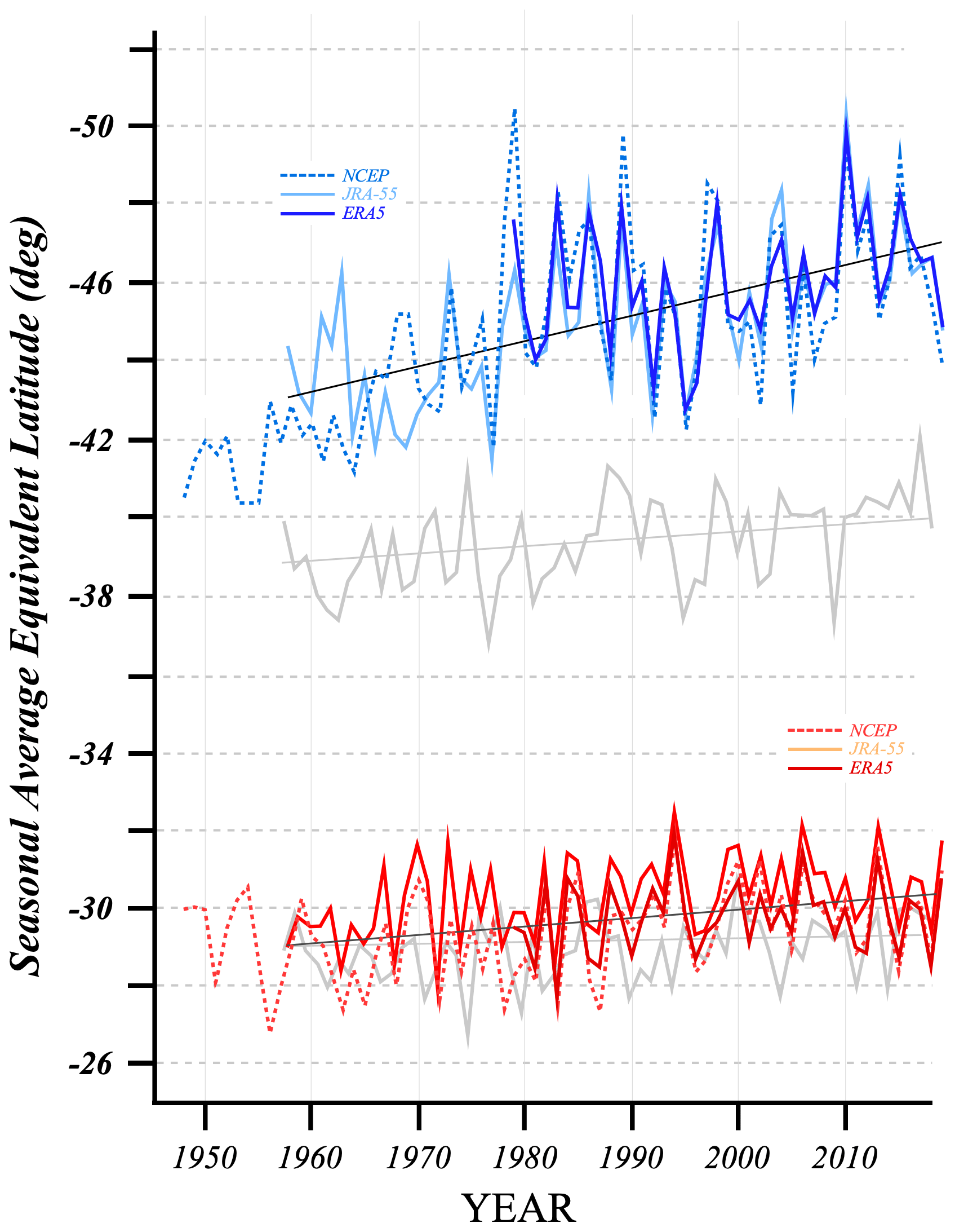
Figure 8 Time series of the seasonal-average equivalent latitude of the polar (blue lines) and subtropical (red lines) jets from the three different SH reanalysis data sets. The thin black lines are the trend lines (from the JRA-55 data) and are significant above the 99 % level for both jet species. Gray lines are the boreal-winter equivalent latitude analysis from Fig. 10 of Martin (2021).

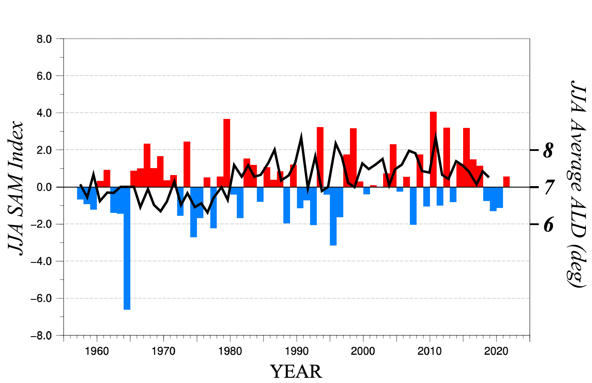
Figure 9 JJA-average SAM index (histogram) from NCEP's Climate Prediction Center. The index is calculated by projecting the daily 700 hPa geopotential height anomalies poleward of 20^∘ S onto the leading pattern of the Antarctic Oscillation (AAO) of Gong and Wang (1999). Black solid line is the JJA-average ALD of the POLJ from the JRA-55 reanalysis.

Next we consider aspects of the analysis in the context of the SAM. Figure 9 shows a histogram of the JJA-average SAM index (calculated after Gong and Wan, 1999) superimposed upon the average JJA ALD from the JRA-55 reanalysis. The tendency toward a positive SAM over the time series appears to be reflected in the increase in ALD. However, the correlation between the two time series is 0.053, suggesting almost no relationship exists between the two.

In order to investigate the relationship of ALD to extremes in the polarity of the SAM index, the 3 winter months with the most positive and most negative SAM extremes since 1979 were considered. The core isertels of the POLJ (from the JRA-55 reanalysis) for each of these 3 months is portrayed in Fig. 10. Positive extremes of the SAM (Fig. 10a, c, and e) show a clear poleward encroachment of the SH polar jet, while negative extremes (Fig. 10b, d, and f) suggest the opposite. There appears to be no systematic connection, however, between extremes in the SAM and the waviness of the POLJ as quantified by ALD.

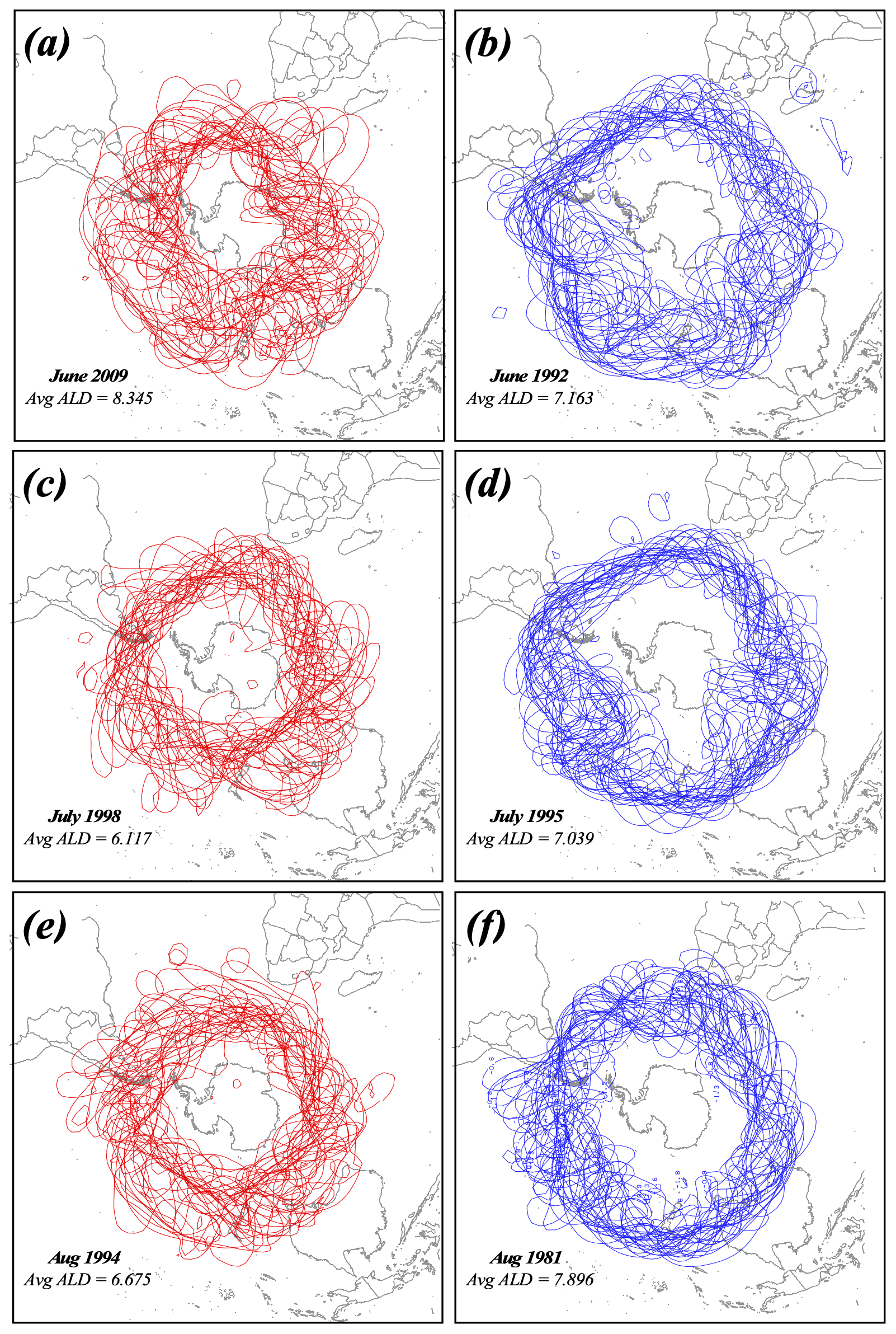
Figure 10 Spaghetti plots of core isertels from SH summer months with maximum positive (red) and negative (blue) SAM indices since 1979. (a) Daily JRA-55 core isertels from June 2009, the June with the most positive SAM in the record. (b) As for Fig. 10a but for June 1992, with June being the most negative SAM in the record. (c) As for Fig. 10a but for July 1998. (d) As for Fig. 10b but for July 1995. (e) As for Fig. 10a but for August 1994. (f) As for Fig. 10b but for August 1981. Average ALD for the given months are listed in the bottom left of each panel.

Thus far the analysis has presented elements of the seasonal-average behavior of the austral-winter jet species. The methodology, of course, allows for evaluation of daily time series of ALD as well, and, in fact, such an analysis underlies the presentation in Fig. 6. Using such daily time series, identification of the waviest and least wavy seasons for each jet species since 1979 is accomplished by summing the daily departures from calendar-day average ALD over the 92 d of each cold season. The list of such seasonally integrated departures from average waviness for each species of jet for each reanalysis data set is shown in Table 1. From this list, the five waviest and five least wavy seasons for each jet species were selected to construct composites of geopotential height at several isobaric levels employing the JRA-55 data. In the foregoing analysis, height differences are obtained by subtracting values associated with the composite least wavy seasons from those associated with the composite waviest seasons.

Table 1 Integrated seasonal departures from average ALD (degrees) for polar and subtropical jets from the three reanalysis data sets employed in this work. Bold (italics) represents one of the top five waviest (least wavy) seasons from 1979–2019.

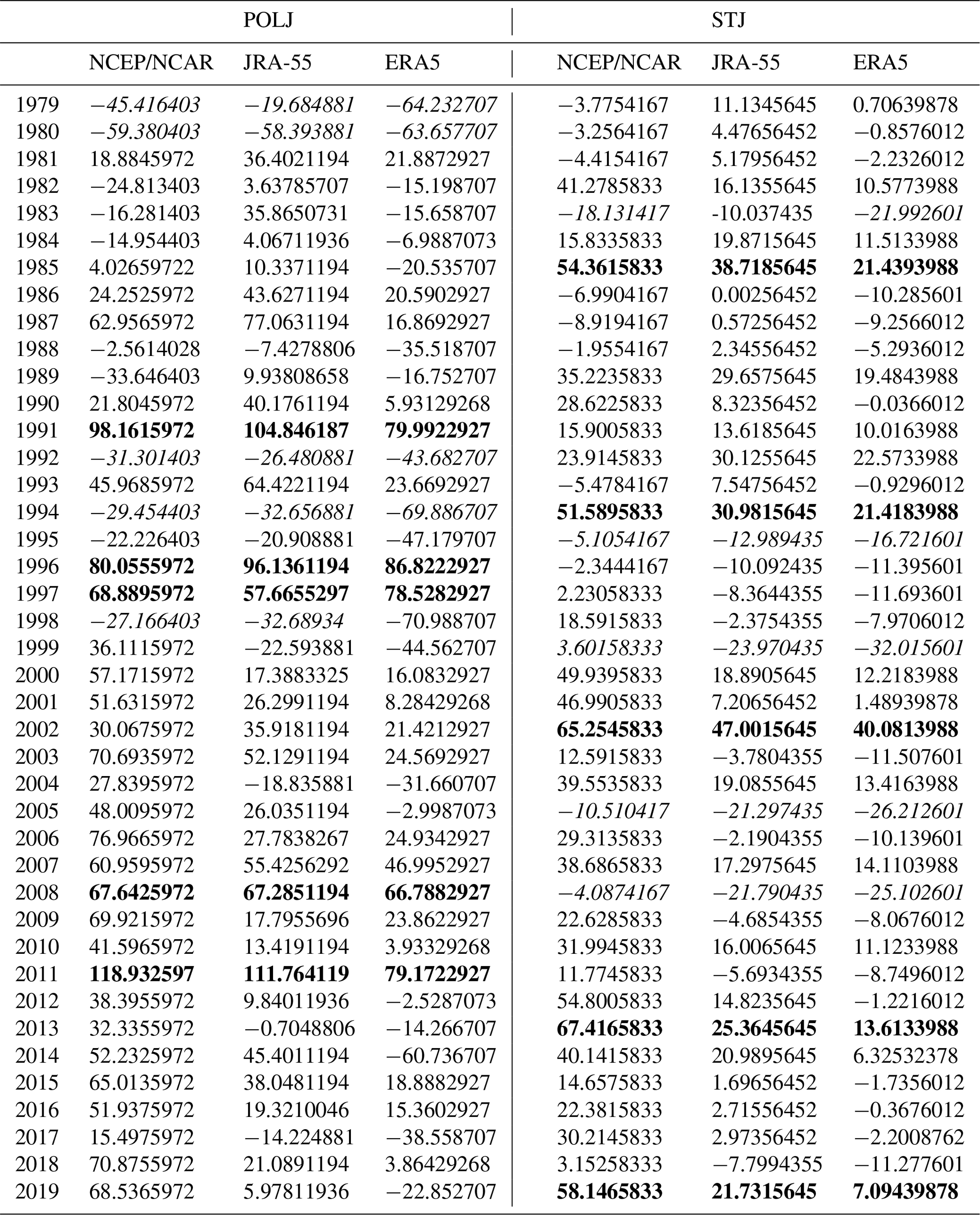
Figure 11a shows the 500 hPa geopotential height differences between the waviest and least wavy POLJ seasons. Wavy POLJ years are characterized by positive height anomalies over the continent and adjacent to its eastern and western coasts with belts of negative anomalies in a crescent beginning in the southwest of Chile and then extending from the eastern coast of South America to southern Africa toward Australia, suggestive of a negative SAM. The strongest negative height anomalies in such seasons occur west of South Africa, implying a slight weakening of the zonal winds just south of the Cape of Good Hope. Meanwhile wavy STJ years exhibit negative composite height differences in roughly the same locations as the positive composite differences just described for wavy POLJ years (Fig. 11b), suggestive of a positive SAM. These composite difference patterns strengthen slightly at 250 hPa (Fig. 12), suggesting an equivalent barotropic structure to the tropospheric portion of the difference fields.

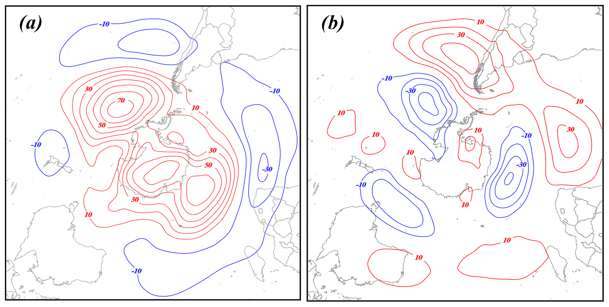
Figure 11 The 500 hPa height differences between the composite waviest and least wavy (a) polar-jet and (b) subtropical-jet seasons constructed from the JRA-55 reanalysis. See Table 1 for identification of the specific years comprising each composite. Positive (negative) height differences are solid red (blue) lines labeled in meters and contoured every 10 m (−10 m) beginning at 10 m (−10 m).

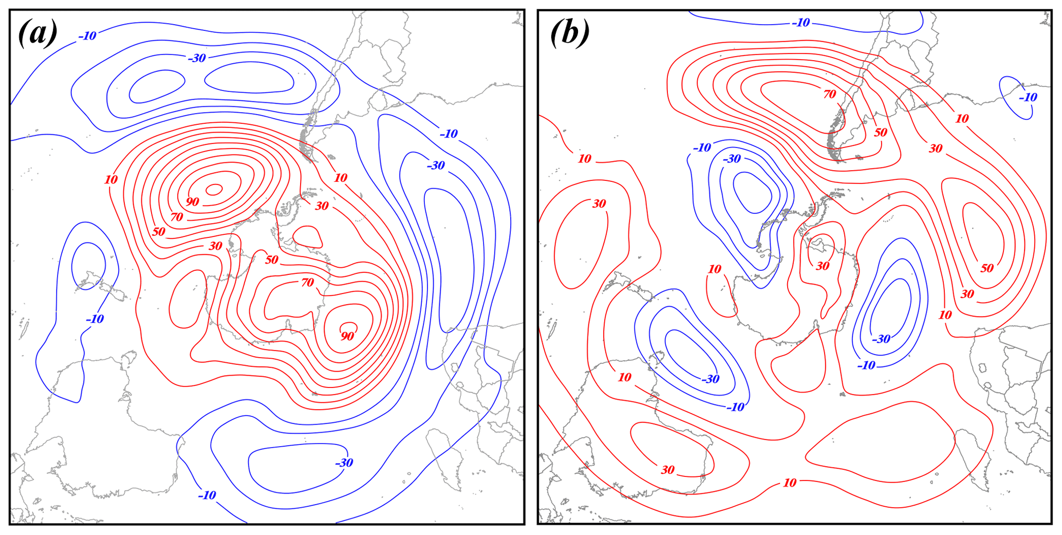
Figure 12 The 250 hPa height differences between the composite waviest and least wavy (a) polar-jet and (b) subtropical-jet seasons constructed from the JRA-55 reanalysis. See Table 1 for identification of the specific years comprising each composite. Positive (negative) height differences are solid red (blue) lines labeled in meters and contoured every 10 m (−10 m) beginning at 10 m (−10 m).

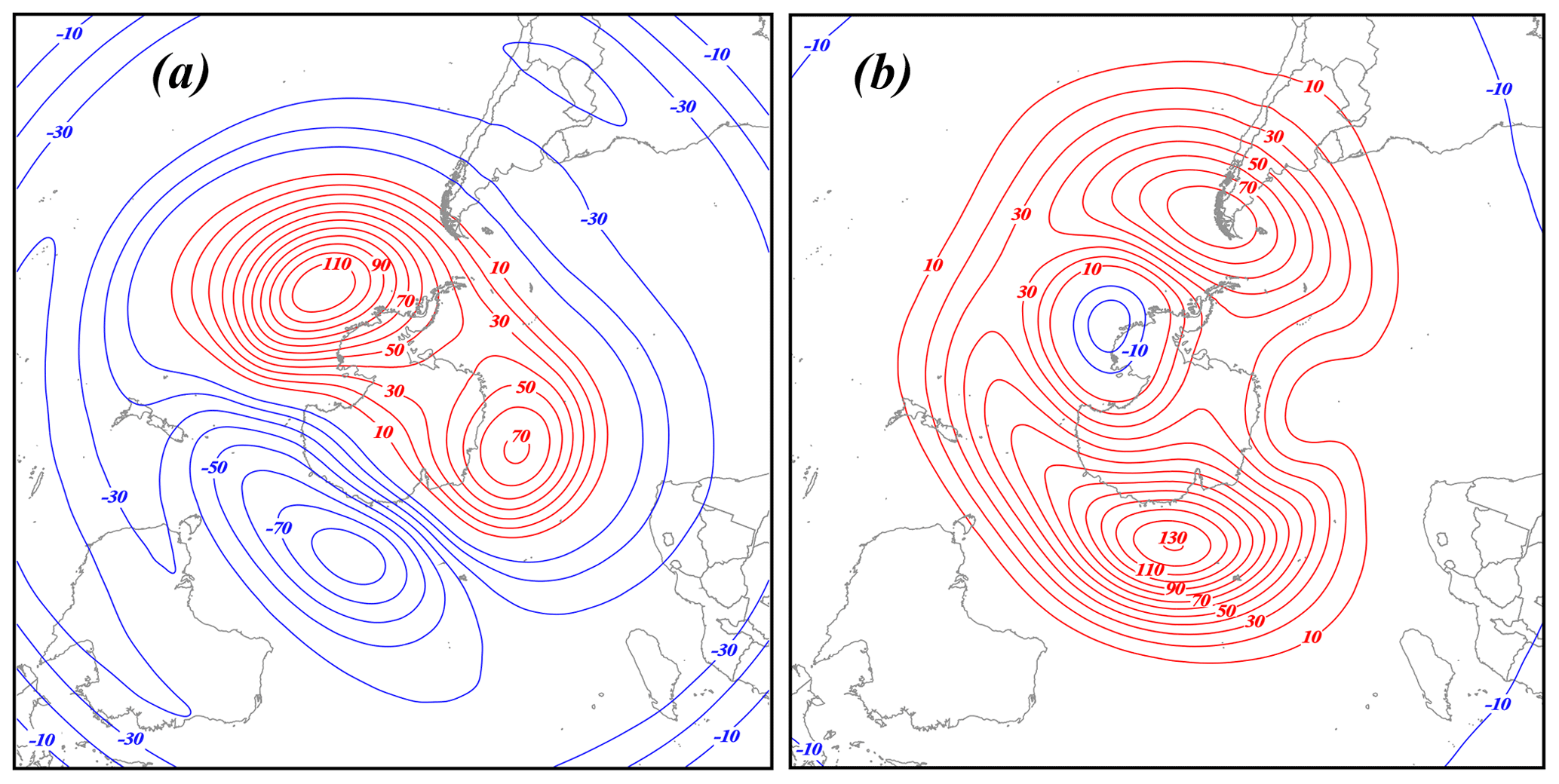
Figure 13 The 50 hPa height differences between the composite waviest and least wavy (a) polar-jet and (b) subtropical-jet seasons constructed from the JRA-55 reanalysis. See Table 1 for identification of the specific years comprising each composite. Positive (negative) height differences are solid red (blue) lines labeled in meters and contoured every 10 m (−10 m) beginning at 10 m (−10 m).

The difference fields at 50 hPa imply that the waviness of both jets exerts an influence on the strength of the austral polar vortex in the lower stratosphere. The anomalous height field associated with wavy POLJ years (Fig. 13a) suggests a broad, though modest, anticyclonic circulation anomaly just off the pole in the Western Hemisphere. Such a perturbation flow would appear to interfere with the establishment and/or persistence of strong vortex flow in the same location. Wavy STJ seasons also impose a dipole of positive heights the axis of which stretches from Cape Horn to East Antarctica (Fig. 13b). Such a configuration implies that the polar vortex is both weaker and displaced off the pole in winters with wavy STJs. Thus, the analysis suggests that in winters characterized by unusually wavy jets of either species, the SH polar vortex is likely weaker than normal. Further investigation of this intriguing implication is the subject of ongoing work.

4 Summary

The analysis presented here extends the application of a method developed by Martin (2021) to assess the waviness of the tropopause-level jets to analysis of the austral-winter polar and subtropical jets. The analysis demonstrates that both jets have become systematically wavier over the past 60+ years. In addition, as in the NH, the waviness of the two species of austral-winter jets is largely uncorrelated, suggesting little systematic influence of one on the other throughout the season. Along with these similarities, there appear to be some fundamental asymmetries in the behavior of the wintertime tropopause-level jets between the hemispheres. The austral POLJ, like its NH counterpart, has exhibited no trend in its average speed over the time series, though it is notably slower than its NH wintertime equivalent. The STJ, on the other hand, has roughly the same speed as that in the NH winter but, unlike its NH counterpart, has undergone a systematic, statistically significant increase in its core speed since about 1960. Additionally, as opposed to the situation in the NH where only the POLJ migration toward the pole is statistically significant, both SH jets exhibit a significant poleward creep with the POLJ encroachment occurring at ∼ 3 times the rate of that characterizing the STJ.

The observed poleward migration of the STJ reported here is consistent with the analysis of CMIP5 (Coupled Model Intercomparison Project) simulations of historical and projected changes to the SH wintertime STJ by Chenoli et al. (2017). Though the present work employs a similarly dynamical definition of the STJ as that used in the study by Maher et al. (2020), they found no evidence of a poleward shift of the SH wintertime STJ. We suggest that the emphasis on empirically identifying a core isertel, rather than the maximum gradient of θ on a predetermined isertelic surface (i.e., 2 PVU as the dynamic tropopause), may account for this difference.

Finally, circulation differences between the waviest and least wavy POLJ and STJ seasons are manifest in both the troposphere and lower stratosphere. In the troposphere the signals are not as coherent in the SH as they were revealed to be in the NH (Martin, 2021). Interestingly, the analysis implies that when either the POLJ or STJ is wavier than normal in a given winter, the lower-stratospheric polar vortex is negatively impacted. Again, this is different from the behavior of the NH polar vortex in the face of extremes in waviness.

The results presented here, combined with those in Martin (2021), demonstrate that in both hemispheres a wavier-than-normal STJ during winter serves to weaken the lower-stratospheric polar vortex. Though, as suggested by the analysis supporting Fig. 6, the STJ and POLJ do not appear to influence one another systematically, there are still instances in which the waviness of the two jets can be phased so as to promote intense interactions. Daily perusal of hemispheric synoptic maps suggests that such instances of jet interaction often lead to intense lower-tropospheric cyclogenesis events. Current research is examining whether such jet-interaction-induced cyclogenesis events from specific seasons systematically correspond to episodes of polar-vortex weakening.