Strengthening gradients in the tropical west Pacific connect to European summer temperatures on sub-seasonal timescales

Recent work has shown that (sub-)seasonal variability in tropical Pacific convection, closely linked to the El Niño–Southern Oscillation (ENSO), relates to summertime circulation over the Euro-Atlantic. The teleconnection is non-stationary, probably due to long-term changes in both the tropical Pacific and extra-tropical Atlantic. It also appears imperfectly captured by numerical models. A dipole in west Pacific sea surface temperatures (SSTs) was found to be the best predictor of errors in numerical sub-seasonal forecasts of European temperature. In this diagnostic study we use reanalysis data to further investigate the teleconnection pathway and the processes behind its non-stationarity. We show that SST gradients associated with the dipole represent a combination of ENSO variability and west Pacific warming, and have become stronger since 1980. Associated patterns of suppressed and enhanced tropical heating are followed by quasi-stationary waves that linger for multiple weeks. Situations with La Niña-like gradients are followed by high-pressure centres over eastern Europe and Russia, three to six weeks later. Inverted situations are followed by high pressure over western Europe, three to six weeks later. The latter situation is conditional on a strong meridional tripole in north Atlantic SSTs and a co-located jet stream. Overall, the sub-seasonal pathway diagnosed in this study connects to patterns detected on seasonal scales, and confirms earlier findings that the summertime connectivity between the Pacific and Europe has shifted in recent decades.

1 Introduction

Sub-seasonal forecasts are made with a lead time of 2–6 weeks. For weather at any mid-latitude location, part of the predictability at that lead time originates in the tropics (Vitart and Robertson, 2018). Tropical deep convection and associated diabatic heating generate upper level divergence and vorticity anomalies that force Rossby waves (Hoskins and Karoly, 1981; Sardeshmukh and Hoskins, 1988; Trenberth et al., 1998). These waves can propagate into the westerly mid-latitude flow and steer associated weather patterns, commonly affecting the mid-latitudes beyond two weeks into the future (Liu and Alexander, 2007; Branstator, 2014; Stan et al., 2017). Impacts on mid-latitude surface weather are especially pronounced when waves are quasi-stationary (Schubert et al., 2011; Wolf et al., 2018; Röthlisberger et al., 2019). An example of a teleconnection from tropical heating is the Madden Julian Oscillation, which is in the Euro-Atlantic sector, has a phase-dependent influence on the North Atlantic Oscillation (Cassou, 2008; Henderson et al., 2017; Vitart, 2017).

Since its origins, teleconnection research has mostly focused on winter, as this is a season with higher baroclinicity and more potent Rossby wave propagation (Bjerknes, 1969; Trenberth et al., 1998; Branstator and Teng, 2017). Teleconnections are also thought to have an influence in summer (Cassou et al., 2005). Heating patterns over the western tropical Pacific are of primary importance for summertime quasi-stationary Rossby waves (QSRWs) (Ting, 1994; Behera et al., 2013; Ma and Franzke, 2021). The dipole of enhanced convective activity over the Maritime continent, in conjunction with reduced activity over the west and central Pacific, is related to circulation over the Euro-Atlantic sector (O’Reilly et al., 2018; Fuentes-Franco and Koenigk, 2020). One feature known for producing such zonal contrasts in sea surface temperature (SST) and atmospheric heating, is the El Niño Southern Oscillation (ENSO). When ENSO's atmospheric component (the Walker circulation) strengthens, convection over the Maritime continent increases and that over the tropical central Pacific decreases (Bjerknes, 1969). It is for instance thought that a (developing) La Niña episode supported the prominent blocking that was part of the Russian heatwave of 2010 (Schneidereit et al., 2012). On the other hand, it is also thought that SSTs had little influence on the Russian heatwave (Dole et al., 2011; Hauser et al., 2016; Wehrli et al., 2019).

Besides the zonally oriented dipole implicated in ENSO, namely between the tropical central Pacific and Maritime continent, meridional orientation is important as well. Diagnosis by Ding et al. (2011) of heating patterns that steer mid-latitude flow reveals that anomalous subtropical heating can relate to QSRWs. Such meridional features reflect activity of the Indian Summer Monsoon and the western north Pacific monsoon, as both consist of anomalous convection extending northward, into the Indian subcontinent and the western north Pacific (WNP) respectively. The SST contrasts in both the zonal and meridional direction have increased rapidly since 1990 by what is called the “west Pacific warming mode” (Funk and Hoell, 2015). This long-term change is diagnosed in SSTs from which the first-order effects of ENSO have been removed and can thus be viewed as change in the “background state” of the Pacific. It consists of concentrated warming over the Maritime continent and the WNP region. This is found to be a response to anthropogenic emissions (Funk and Hoell, 2015) and has strengthened the Walker circulation (Funk et al., 2018; Lee et al., 2022).

Coinciding with west Pacific warming, observed connectivity between the Pacific and Euro-Atlantic circulation appears to have strengthened (O'Reilly et al., 2019; Sun et al., 2022). This strengthening is not a consequence of internal atmospheric variability but is a response to the SST trends (O'Reilly et al., 2019), potentially influencing current and future Euro-Atlantic circulation. Unfortunately, numerical climate models seem unable to reproduce the observed changes in Euro-Atlantic circulation (Boe et al., 2020; Vautard et al., 2023), meaning that they underestimate the rapid increase of European summer temperature extremes (van Oldenborgh et al., 2022). Also, numerical weather prediction (NWP) models have shortcomings in simulating Rossby wave teleconnections (O’Reilly et al., 2018; Quinting and Vitart, 2019). We previously found that west Pacific SSTs could relate to QSRWs that conditionally led to monthly European summer temperature anomalies. This teleconnection appeared imperfectly represented in the numerical model of the European Centre for Medium-range Weather Forecasts (ECMWF) (van Straaten et al., 2023).

The shortcomings of weather- and climate-models can reside in many processes associated with Rossby wave teleconnections. Whether QSRWs influence a remote location can be modulated by processes related to the forcing of waves, and processes related to wave propagation and amplification (White et al., 2022). In the Pacific region, or further along the propagation trajectory, other sources of heating and vorticity can strengthen the QSRW when they are in-phase, and negate it when they are out-of-phase, dependent on the optimal forcing pattern of the QSRW (Schubert et al., 2011; Kim and Lee, 2022). Extra-tropical Pacific SST anomalies provide such feedback when preceding dynamics have left in place an anomaly pattern that is in-phase with a summertime QSRW (Vijverberg and Coumou, 2022). In the same way the state of the north Atlantic can permit or hinder QSRW propagation towards Europe (Fuentes-Franco et al., 2022). Also, soil moisture depletion, for example over the US, can amplify wave patterns and make them circumglobal (Teng and Branstator, 2019).

A second potential modulator is the way in which atmospheric jets function as waveguides (Hoskins and Ambrizzi, 1993; White et al., 2022). Waveguides are sharp gradients in the background flow, along which Rossby waves propagate (Wirth et al., 2018; Manola et al., 2013). The role of jets is noticeable as strong waves often emanate at their exit regions, of which the Euro-Atlantic sector is one (Stan et al., 2017). The characteristics of the background flow, in the form of jet position, width, and strength, can determine whether a wave response will be of limited longitudinal extent, or circumglobal (Branstator and Teng, 2017).

In this study we characterize the west Pacific teleconnection to European summer temperature variability and evaluate whether the teleconnection relates long-term changes in the Pacific to Euro-Atlantic circulation. To that end we build an index for an SST dipole over the west Pacific, and an index for European surface temperature more than two weeks later. Such a lagged, sub-seasonal timeframe is different from the concurrent, seasonal diagnostics used in earlier studies (Ding et al., 2011; Behera et al., 2013; O’Reilly et al., 2018). We assess the apparent strengthening of teleconnection and investigate whether it is modulated by (a combination of) the processes described above. Overall, we hope that our diagnostic framework can aid the inspection of this teleconnection in weather- and climate-models, such that long-term projections and sub-seasonal forecasts of European summer extremes can ultimately be improved.

2 Data

In this study we use the ERA5 reanalysis (Hersbach et al., 2020). We extract daily values of SST and two-metre temperature (t2m), as they will form the respective start- and end-points of the teleconnection. Top-of-the atmosphere outgoing longwave radiation (OLR) was extracted as indicator of tropical deep convection, zonal wind at 300 hPa (u₃₀₀) as an indicator of jet stream strength and position, and geopotential height at 300 hPa (z₃₀₀) as an indicator of the QSRW itself. Values were extracted from 1950 until 2021, in a domain that spans from 20^∘ S to 90^∘ N, and 180^∘ W to 180^∘ E, at a spatial resolution of 0.25 × 0.25^∘.

Daily values were de-seasonalized by approximating the seasonal cycle with a polynomial that is a function of the day-in-the year (as in Mayer and Barnes, 2021, 2022). We found that a 7th order polynomial was most suited to accommodating the changing shape of seasonal cycles with latitude. For polynomials with orders lower than 5 the residuals remained visibly dependent on the season. For each grid cell the polynomial was fitted to the complete set of years from 1950 to 2021. Daily anomalies of all variables were then averaged to four-week (28 d) values. In previous studies we namely found that the four-week or “monthly” average t2m is predictable with sub-seasonal lead times (van Straaten et al., 2022, 2023). The aggregation is executed as a rolling-window averaging, such that one value was recorded each day.

The WNP region, whose warming as part of the west Pacific warming mode was found to have a strong influence on the Walker circulation, is defined from 10–30^∘ N 130^∘ E–170^∘ W (Funk et al., 2018). In this region we record each day the spatial mean, four-week average SST anomaly.

To investigate the role of ENSO we use pre-computed monthly relative ENSO indices (van Oldenborgh et al., 2021), based on the ersstv5 dataset of ocean observations (Huang et al., 2017), in regions Niño 3 (5^∘ S–5^∘ N, 90–150^∘ W) and Niño 4 (5^∘ S–5^∘ N, 160^∘ E–150^∘ W) (Trenberth and Stepaniak, 2001). Relative ENSO indices are computed like regular ENSO indices as the average SST anomaly within a Niño region (climate normals defined from 1981 to 2010), but from which the average SST anomaly between 20^∘ N and 20^∘ S is subtracted. This makes the indices less distorted by global warming and more useful for describing teleconnections (van Oldenborgh et al., 2021). We interpolate them linearly to obtain a monthly value each day.

For the Pacific Decadal Oscillation (PDO) we use standardized values of the first principle component of monthly Pacific SST anomalies north of 20^∘ N (Mantua et al., 1997). The pre-computed index is provided by the National Oceanic and Atmospheric Administration (NOAA) and is also based on ersstv5. We interpolate the PDO index linearly to obtain a monthly value each day.

As mentioned, we previously found that the average t2m anomaly is predictable when aggregated to the four-week or “monthly” timescale (van Straaten et al., 2022). Crucially, this predictand involved spatial averaging as well. Sub-seasonal predictions for individual grid cells are usually less successful, because only the overarching variability that affects daily anomalies at multiple moments and locations can be predictable (Buizza and Leutbecher, 2015; Wheeler et al., 2017; van Straaten et al., 2020). In the mentioned previous study we used hierarchical clustering to find a west and central European region (Fig. 1b), in which the average t2m anomaly is predictable (van Straaten et al., 2022). For the remainder of this study we refer to this predictand as “Western European t2m” in weeks 3, 4, 5, and 6. A diagnostic plot of June–July–August (JJA) averages of this variable shows that summer temperatures have been warming (Fig. 1a). In fact, western European summer temperatures have been warming faster than the global average, especially since the 1990s, at a rate of 0.4 to 0.8 ^∘C/decade (Christidis et al., 2015; Dong et al., 2017; Gutiérrez et al., 2021).

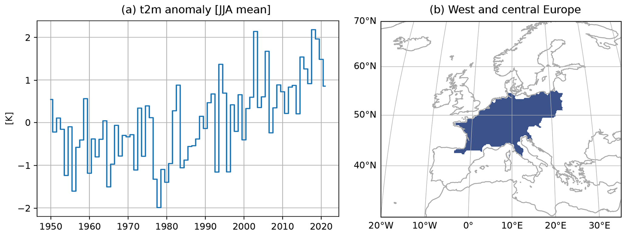
Figure 1 Two-metre temperature (t2m) anomaly in west and central Europe. (a) Seasonal mean (June–July–August, JJA) ERA5 t2m anomaly in the region, from 1950 to 2021. (b) west and central European region.

3 West Pacific dipole index

Figure 2 displays Pacific SST grid-cells whose variability precedes European t2m by more than two weeks. We correlate four-week-averaged SST anomalies (“SST in weeks −3 to 0”) to the lagged European four-week-averaged response (“t2m in weeks 3 to 6”). Our use of rolling averages leads to 92 samples per JJA season. The gap of two weeks between the two periods corresponds to the time window over which tropical Rossby waves still affect the mid-latitudes (Branstator, 2014) (alternative lags are discussed in Appendix A). The presented correlation is corrected for inflating factors like global warming and auto-correlation (Fig. 2a). Specifically, we compute the partial correlation between residual SST and residual t2m. First, we let a linear regression predict observed SST and t2m anomalies using time and the value of the previous time step (details can be found in van Straaten et al., 2022). These predictions are then subtracted from the observed anomalies, resulting in residual SST and t2m. With the confounding effects of global warming and auto-correlation removed, any correlation that remains significant is more likely to represent a sub-seasonal relation. The significance of the partial correlation is determined per grid cell by a two-sided test with nominal level ($\mathit{\alpha }=\mathrm{5}\cdot {\mathrm{10}}^{-\mathrm{12}}$) (this small α was a pragmatic way of accounting for the dependence introduced by rolling window averaging). To mitigate the accumulation of chance-based discoveries when performing multiple significance tests, we applied a false discovery rate correction (Benjamini and Hochberg, 1995) (details can be found in van Straaten et al., 2022). Within the full dataset of 1950 to 2021, we further test robustness of the partial correlation with a five-fold cross validation, leaving out consecutive blocks of 14 years. Grid cells with correlations significantly different from zero in five out of five subsets are highlighted in yellow (Fig. 2b).

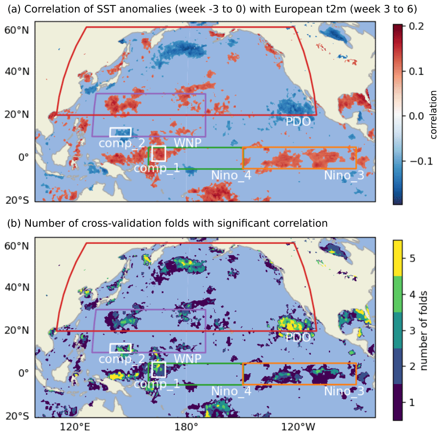
Figure 2 Connection between ERA5 Pacific sea surface temperature (SST) anomalies and European two-metre temperature (t2m) anomalies on sub-seasonal timescales in summer (1950–2021). (a) Spearman rank correlation between week −3 to 0 SST anomalies and week 3 to 6 western European t2m, corrected for inflation by linear trends, seasonality and auto-correlation. Reported is the mean correlation over five cross validation folds, constructed by leaving out consecutive blocks of 14 years. (b) Robustness of the correlation as measured by the number of folds with significant correlation. Annotated are regions commonly used to capture Pacific variability. The two components of the west Pacific Dipole (WPD) index are highlighted by white squares. PDO, Pacific Decadal Oscillation; WNP, western north Pacific.

The highlighted SST regions relate to European t2m, and do not correspond perfectly to patterns that explain the highest amount of Pacific variability, like PDO and ENSO. Aspects are however captured. A large cluster of significant cells resides in the region used to define the PDO (Mantua et al., 1997) (Fig. 2b). Also, at the western edge of the Niño 4 area, we see a cluster of cells (called “component 1”, 1.5^∘ S–5.5^∘ N, 162–169^∘ E). This cluster is flanked by “component 2” (10–14^∘ N, 140–150^∘ E), which lies within the WNP area (Fig. 2). These regions were the focus of the study by van Straaten et al. (2023), showing that the opposed sign of anomalies in these two regions, when captured with a spatial co-variance predictor, were important and related to errors in the ECMWF model. The respective positive and negative correlations of components 1 and 2 (Fig. 2a) hint at situations with anomalously warm SSTs in component 1 and anomalously cold SSTs in component 2, and in which weeks 3 to 6 European t2m would later be above normal (and vice-versa). This emphasizes the importance of the western Pacific in forcing a teleconnection towards Europe (as seen in Ding et al., 2011; Behera et al., 2013; O’Reilly et al., 2018; Ma and Franzke, 2021). Furthermore, with component 2 located in the WNP and component 1 at the eastern edge of the central Pacific, their combination appears to capture a heating contrast with both meridional and equatorial orientation (i.e. the emphasized signal consists of more than just zonally opposing anomalies along the equatorial axis).

Here, we simply capture this contrast by defining a west Pacific Dipole (WPD) index, namely the four-week anomaly in component 1 minus the four-week anomaly in component 2. As SSTs in component 2, which is further west in the Pacific, are, in absolute terms, generally warmer than those in component 1, this definition dictates that positive WPD values represent a weakening of the climatological SST gradient, and negative WPD values represent a strengthening of the climatological gradient. The reason why positive WPD is defined as “positive” is its association with above-normal western European t2m (Fig. 3c).

To test the sensitivity of choices regarding the location of the two boxes, we present additional results in Appendix A. These are additional cross validation maps, similar to Fig. 2b, and show that the exact extent and location of the robustly correlated pattern can shift when different combinations of timescales and lags are chosen. The current boxes are positioned such that only the features shared among multiple combinations are captured.

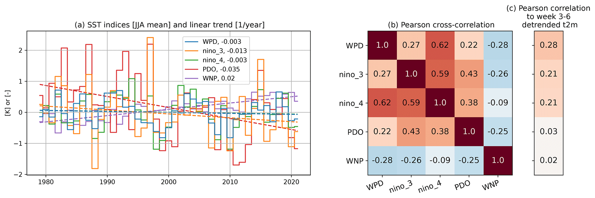
Figure 3 Correspondence between the west Pacific Dipole (WPD) index (sea surface temperature, SST, in “component_1” minus SST in “component_2”, Fig. 2), and other Pacific indices. (a) Seasonal mean timeseries and linear trend from 1979 to 2021. (b) Cross-correlation matrix between the SST indices (June–July–August, JJA, only). (c) Lagged correlation between SST indices and European t2m in weeks 3 to 6, corrected for a linear trend in t2m. The SST indices capture SSTs from week −3 to 0 (see also Sect. 2). Shading in (b) and (c) illustrates the sign of the reported correlation values (red: positive, blue: negative) and their magnitude (dark: strong, light: weak). PDO, Pacific Decadal Oscillation; WNP, western north Pacific.

We expect the WPD index to relate to other Pacific modes. PDO for instance, comprises a combination of remote ENSO-induced variability in combination with local atmosphere-ocean interactions (Newman et al., 2016). Especially due to spatial overlap in regions, we see that WPD relates to Niño 4 and WNP, which is illustrated by cross-correlations of 0.61 and −0.29 respectively, in the period from 1979 until 2021 (Fig. 3b). (We do not include the pre-1979 period because it lacks the west Pacific warming mode and the stronger Pacific–Atlantic connections, Funk and Hoell, 2015; O'Reilly et al., 2019, which would muddy the illustration of current inter-relations.) The real difference with for instance Niño 4, is that the WPD index is designed to specifically target the teleconnection towards Europe, which is confirmed by the highest correlation of all indices with weeks 3–6 t2m (Fig. 3c).

Correlation between Pacific modes is further illustrated by a year-to-year representation of the time series (Fig. 3a). Over the 1979–2021 period the standardized PDO is moving towards a negative phase (−0.031 std yr⁻¹). Also, Niño 3 displays a slight negative trend (−0.013 K yr⁻¹), which is different from Niño 4 and WPD, and opposed to the positive trend in WNP (0.02 K yr⁻¹). These opposing trends reflect documented warming in the western Pacific, whereas the central to eastern tropical Pacific has not warmed (Wills et al., 2022; Seager et al., 2022; Sun et al., 2022; Lee et al., 2022). The result is that the zonal SST gradient over the tropical Pacific has increased, which is generally referred to as a “La-Niña-like” change in the Pacific “background state”, and has been linked to a stronger Walker circulation (Lee et al., 2022; Seager et al., 2022). Also, the west Pacific warming mode, visible as the warming in the WNP region, enhances the climatological background-gradient over the Pacific, and is linked to a strengthening of the Walker circulation (Funk and Hoell, 2015; Funk et al., 2018), with potentially important influences on tropical–extratropical teleconnections (Schubert et al., 2014; O'Reilly et al., 2019; Sun et al., 2022).

4 Emergence of a teleconnection

We classify the WPD index into three tercile-based categories. The positive phase is when SSTs during weeks −3 to 0 are anomalously warm in component 1 and anomalously cold in component 2. In the negative phase this is inverted, and a neutral phase is in between. Because the WPD index does not have a significant trend (Fig. 3a, −0.003 K yr⁻¹), we determine tercile thresholds over the entire 1950–2021 dataset. Weeks 3–6 t2m, on the other hand, shows a clear trend (Fig. 1a). This trend can be due to a combination of thermodynamic and dynamic processes that can be both of forced and/or unforced origin (see e.g. Deser et al., 2016; Faranda et al., 2023). Since this study focuses on the sub-seasonal connection between WPD and Euro-Atlantic circulation we remove the long-term warming trend by computing t2m tercile thresholds per rolling time window of 21 summers. If not, the upper tercile “positive” t2m class would mostly consist of samples from recent years. With the distortion removed we can define our measure of teleconnection strength or “sub-seasonal connectivity” as: the number of occasions with (i) positive WPD AND positive t2m response, plus the number of occasions with (ii) negative WPD AND negative t2m response. A window length of 21 summers was deemed sufficiently short to adapt to non-stationarity in the roughly 72-year dataset, but sufficiently long not to be affected by inter-annual variability.

Temporal evolution of the WPD classes reveals that since 1950 (the beginning of the dataset) the negative WPD phase has strongly increased in frequency (blue line in Fig. 4a). Until 2000 this happens mostly at the expense of the neutral phase, and after that also at the expense of the positive phase. The dwindling occurrence of the neutral phase can explain why the tercile distribution shows large changes (Fig. 4a), whereas the seasonal mean of WPD had no significant trend (Fig. 3a). The increased occurrence of negative WPD phases does agree with WNP warming and the strengthening of climatological gradients over the Pacific (Sect. 3, Fig. 3a).

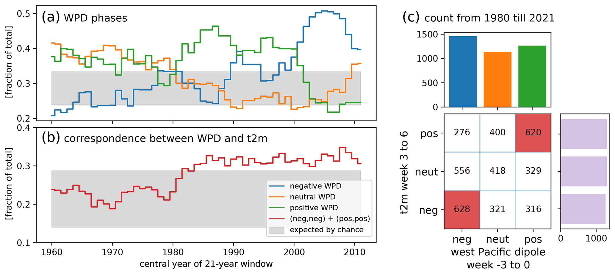
Figure 4 Teleconnection between weeks −3 to 0 west Pacific Dipole (WPD) index and weeks 3–6 European two-metre temperature (t2m), as measured by correspondence in tercile classes (negative, neutral, positive). (a) Prevalence of the three WPD classes in a moving window of 21 summer seasons (blue: negative WPD; orange: neutral WPD; green: positive WPD), with tercile thresholds determined over the entire dataset, from 1950 to 2021. Presented as a fraction of the total number of samples within each 21-year rolling window. (b) Summed occurrence of the negative and positive phases of the teleconnection, i.e. a negative WPD preceding a negative t2m response plus a positive WPD preceding a positive t2m response, as counted for each 21-season window, whereby the t2m tercile thresholds are re-computed in each window. Grey areas in (a) and (b) denote the 0.025 and 0.975 quantiles of the uncertainty distribution when counting is performed on 21 summer seasons that are randomly sampled from the 1950–2021 dataset (500 repeats, with replacement). (c) Distribution of tercile classes for WPD (x axis) and European t2m (y axis) as counted for each 21-season window from 1980 to 2021 (central years 1990–2011) when the teleconnection (both in the negative and in the positive phase) was present in a statistically significant way (as shown in b).

Concurrent with this development we see that lagged t2m phases in weeks 3 to 6 increasingly follow the WPD phases in weeks −3 to 0. The sum of positive and negative responses to positive and negative WPD respectively rises beyond values found by chance (grey area, Fig. 4b). This roughly occurs for 21-year windows centred in 1990 and beyond, meaning that it starts in 1980. The emergence of a significant teleconnection between the Pacific and Euro-Atlantic circulation is reported by other studies, both for the past decades (Wu and Lin, 2012; Lim et al., 2019; O'Reilly et al., 2019; Sun et al., 2022), and for the near-future (Mayer and Barnes, 2022).

In the remainder of this paper we focus on the period 1980–2021, in which a significant teleconnection emerged. The joint distribution of WPD and t2m phases is given in Fig. 4c. Presented are the number of samples in each category (because of rolling averaging one sample per summer day). Note that the marginal distribution of t2m is uniform, because tercile thresholds are re-estimated in each rolling 21-year window, and that the marginal of WPD is not uniform and shows the relative dominance of negative WPD phases in this period.

5 Forcing, quasi-stationary wave, and surface imprint

We now investigate the spatial and temporal patterns that occur during the period in which the teleconnection is significant. Different components of the pathway (i.e. SST, OLR, z₃₀₀, t2m) are plotted as rows in Fig. 5. The negative phase, positive phase and their difference are plotted in the left, right, and middle columns respectively. Unmasked grid cells in the middle column display differences that were found to be significantly different from differences that can arise by chance. To conduct this two-sided test we resampled entire summer seasons from the 1980–2021 data, with replacement (i.e. a block-bootstrap), until groups with sizes as in Fig. 4c were obtained. We then computed the difference between their composite means and repeated the procedure 500 times to obtain a sampling distribution per grid cell. Subsequently, we tested whether the actual difference fell outside the distributions' empirical quantiles (q0.025 and 0.975 for α=0.05, and q0.05 and 0.95 for α=0.1).

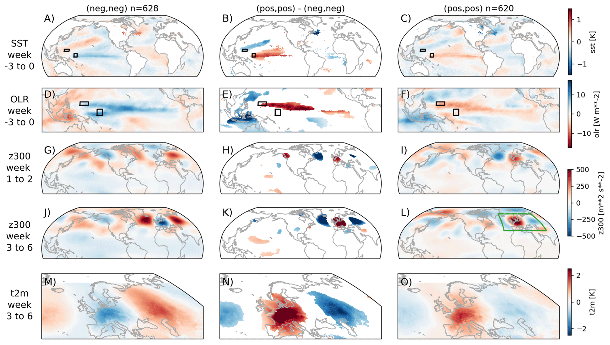
Figure 5 Composite plots illustrating the teleconnection between weeks −3 to 0 west Pacific sea surface temperature (SST) and weeks 3 to 6 west-central European two-metre temperature (t2m), based on composite anomalies from the period 1980–2021 (climate normal also estimated from 1980 to 2021). Left column: samples in which negative west Pacific Dipole (WPD) phases precede the negative t2m class (n=628). Right column: samples in which positive WPD phases precede the positive t2m class (n=620). Middle column: difference between panels in the right and left columns. Values found to not exceed the difference as expected by random chance are masked (α=0.05, more detail in Sect. 5). From top to bottom: SST pattern and outgoing longwave radiation (OLR) in weeks −3 to 0, the subsequent z₃₀₀ response in weeks 1 and 2, and the eventual impact on z₃₀₀ and surface temperature in weeks 3 to 6. Black insets in (a–f) show the two components of the WPD index. Green inset in (l) serves as reference for the spatial extent of surface t2m in the bottom row.

It is clear that the WPD index captures a large geographical pattern with pronounced SST and OLR anomalies across the Pacific ocean, despite being defined by small boxes (Fig. 5a–f). Visually, the SST states in weeks −3 to 0 represent a combination of three patterns: (i) ENSO, which is visible in the La-Niña-like equatorial contrast between anomalously cool SSTs in Niño 4 and anomalously hot SSTs around the Maritime continent in Fig. 5a, and in the El-Niño-like contrasts in Fig. 5c, (ii) the west Pacific warming mode, which Funk and Hoell (2015) describe as a tilted “V” that connects the above-normal SSTs around the Maritime continent to the extra-tropics, in north-eastward and south-eastward directions (the north-eastward extension from component 2 is significantly present in Fig. 5b), and (iii) a PDO-like pattern consisting of the same north-east extension of warm SST anomalies, surrounded by cold anomalies to its south, west, and north, which is a Pacific configuration known to provide summertime predictability for the eastern US (our Fig. 5a and Fig. 1f of Vijverberg and Coumou, 2022). Generally, patterns of SST anomalies captured by WPD resemble the results of the mentioned studies only partially. For instance, the “cold surrounding”, which is part of the PDO-like pattern, does not show up as statistically significant in this study. Such differences are understandable because the WPD index is designed for direct sub-seasonal association with summertime European t2m, which, only to a lesser degree, is found in the other modes (Fig. 3c). The important WPD features, emphasized by significance testing, are the tropical central-to-west Pacific SST anomalies, and the ones in the WNP region, extending north-eastward from component 2 (Fig. 5b).

In OLR we see that the WPD phases correspond to inverted patterns of anomalous deep convection, which need not be aligned with the dipole in anomalous SST and the WPD boxes themselves (Fig. 5d–f). Like SST however, the heating patterns during weeks −3 to 0 consist of an opposition with both equatorial and meridional orientation. Focusing for instance on positive WPD phases, the heating over the Maritime continent and in the western north Pacific monsoon region (north-east of the Philippines) is reduced, and the heating over the central Pacific is enhanced (Fig. 5e–f). This opposition matches the first mode of summertime tropical precipitation variability that was earlier found to be important for steering mid-latitude circulation (Ding et al., 2011). The main difference with the analysis of Ding et al. (2011) is that their analysis diagnosed a concurrent seasonal link, whereas our results suggest that it consists of an underlying, lagged, and sub-seasonal relation (see also Appendix A).

The forcing in weeks −3 to 0 translates into an initial atmospheric response in weeks 1–2 (Fig. 5g–i). Centres of action (locations with the largest z₃₀₀ anomalies) are found from the north Pacific to Eurasia, showing the considerable longitudinal extent of the QSRW (Fig. 5h). Characteristic and significant centres are the high-pressure anomalies in north-west US and the low-pressure anomalies situated south of Greenland and west of the British Isles (Fig. 5i), and which are inverted in the negative phase (Fig. 5g). These centres are part of summertime patterns diagnosed both with a focus on the US heatwaves (Vijverberg and Coumou, 2022) and with a focus on the Euro-Atlantic circulation (Wulff et al., 2017; O’Reilly et al., 2018). As the latter studies used variance decomposition methods (in contrast to our WPD- and t2m-based compositing), the centres found appear to be robust across methods. An interesting difference is that the tropical forcing of the south of Greenland cyclonic anomaly was thought to come primarily from the Eastern Pacific and Caribbean (Wulff et al., 2017), but our results indicate the possibility of west Pacific forcing as well.

After development in weeks 1 to 2, it is clear that the Rossby wave comprising the teleconnection is quasi-stationary, as its lifetime extends into weeks 3 to 6 (Fig 5j–l). This results in negative t2m anomalies in west and central Europe when WPD was negative and positive t2m anomalies when WPD was positive (Fig. 5m, o). In the negative phase a cool western Europe (relative to the climate normal from 1980 to 2021) is flanked by high pressure and high t2m in Eastern Europe and Russia (Fig. 5j, m). This cold-warm t2m dipole has been reported by earlier studies as well (Behera et al., 2013). In fact, given that the negative phase of WPD has been occurring more frequently since 1990 (Fig. 4a), we expect that in recent summers this t2m dipole pattern has become more frequent, which is exactly what Lee et al. (2017) have reported.

6 Modulation

As above, we can look at corresponding WPD and t2m phases and study the teleconnection pathway when it is fully present. But we are also interested in cases where positive or negative WPD phases produce Pacific heating contrasts, but where the full atmospheric response is lacking and the QSRW fails to reach Europe because of a modulating process.

The influence of ENSO on the large-scale background circulation might be such an indirect modulator (Ding et al., 2011; Schneidereit et al., 2012; O'Reilly et al., 2019). An example is the cooling of the atmosphere in the entire tropical belt by a strong La Niña episode. This changes the zonal mean equator-to-pole gradient and therefore the waveguide (Ding et al., 2011). Modulation by ENSO can also happen in a zonally asymmetric way by strengthening the western north Pacific monsoon, or Indian Summer Monsoon (Ding et al., 2011; Di Capua et al., 2020). The evolution of ENSO, i.e. whether it is strengthening, decaying, or persisting, is important as well (e.g. Jong et al., 2020). Strong expression of a pattern in the preceding winter can namely leave an imprint on extra-tropical SSTs, which leads to favourable or unfavourable diabatic interaction with QSRWs in subsequent seasons (Vijverberg and Coumou, 2022).

We investigate whether positive and negative phases of the summertime teleconnection occur under distinct ENSO evolutions, particularly focusing on ENSO evolution in the central to eastern Pacific (Niño 3), which is less directly related to our WPD index (Fig. 3b). Plotted in Fig. 6 is the monthly mean evolution of the relative Niño 3 index in each combination of phases (negative WPD phases in blue, positive WPD phases in red, with opacity denoting whether or not we see a European t2m response). As expected, positive and negative WPD phases are El-Niño-like and La-Niña-like, respectively (red lines are generally on top of blue lines, Fig. 6). This differentiation between red and blue actually increases when moving from preceding December–January–February (DJF), via JJA (zero on the x axis), to subsequent DJF. This confirms that summers with a strong forcing pattern, in our case the non-neutral WPD phases, relate to the strengthening of ENSO (Ding et al., 2011): The negative summertime WPD phase occurs during years when ENSO migrates from an average neutral state to a pronounced La Niña state. Vice versa, the positive WPD phase occurs when ENSO migrates from an average neutral state to an El Niño state. This does not imply that ENSO also fully determines the resulting t2m response. A negative t2m response is likely after a negative WPD phase (and vice versa) given the significance of the teleconnection (Fig. 4c). But within each WPD group (comparing blue lines of different opacity, and red lines of different opacity), there are no distinct ENSO states related to the “pos,pos” (darkest red) and “neg,neg” (lightest blue) teleconnection occurrences (Fig. 6).

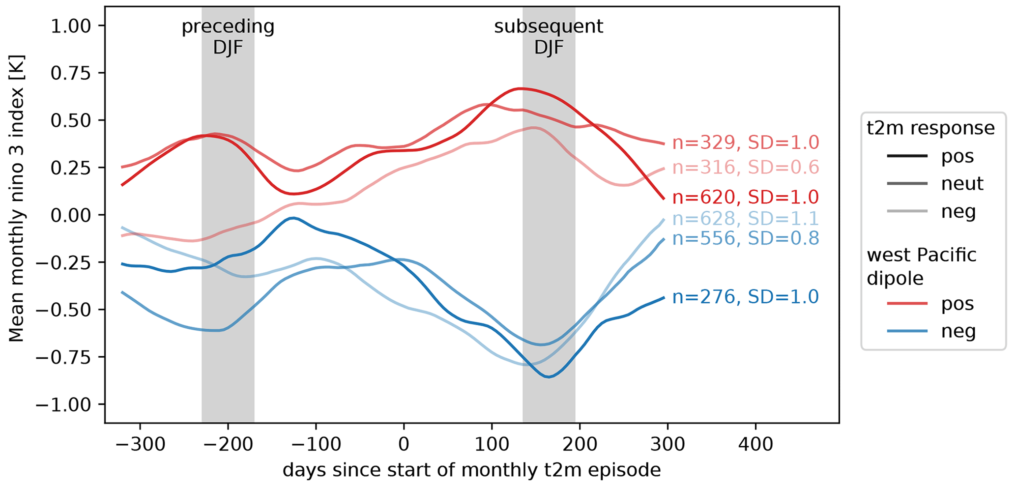
Figure 6 Evolution of the monthly mean relative Niño 3 index, computed per group of samples (determined in June–July–August, JJA). Plotted are groups with positive (red) and negative (blue) WPD phases (based on the sea surface temperature anomaly in weeks −3 to 0, sometime in JJA). The phases tend to occur when the El Niño-Southern Oscillation (ENSO) evolves from neutral to El Niño or La Niña. Plotted with opacity is the European two-metre temperature (t2m) response in weeks 3 to 6 (a moment in JJA that we set to zero on the x axis). This response seems independent of the ENSO state. Samples come from the period 1980–2021. Grey boxes indicate moments that are guaranteed to fall in winter (December–January–February, DJF), as this depends on whether x=0 occurs early or late in summer. Number of samples and standard deviation of DJF values are annotated per group.

If not by ENSO, the QSRWs from west Pacific heating anomalies can also be modulated by other factors. For negative teleconnection phases little was found, but for positive WPD phases we plot the spatial composite patterns of SST and u₃₀₀ (Fig. 7). The composite plots show the state in weeks −3 to 0, so before the QSRW occurs, and show the developing QSRW itself with z₃₀₀ in weeks 1 and 2, with on the left samples leading to a lagged, positive European t2m response, and on the right all those that do not. The middle column shows that with a similar Pacific WPD state, SST patterns are hardly significantly different, except for a branch of warm Atlantic SSTs extending north-east from the Caribbean (Fig. 7b). The warm branch is part of a meridional cold-warm-cold tripole in the north Atlantic that is associated with positive t2m responses (Fig. 7a). Diagnosed by earlier studies, this tripole pattern relates to the strength of the oceanic gyres in the north Atlantic, which are partly driven by wind-stress on the ocean surface (Häkkinen et al., 2011). In the configuration of Fig. 7a, cyclonic circulation and cold SSTs prevail south of Greenland, where heat is transferred from ocean to atmosphere (Häkkinen et al., 2011). The tripole pattern spans multiple seasons and can occur as early as late winter and early spring. From that moment onwards it is known to precede the summertime pattern with a strong low pressure anomaly positioned south of Greenland and west of the British Isles (Fig. 5g) (Gastineau and Frankignoul, 2015; Ossó et al., 2020; Wolf et al., 2020; Beobide-Arsuaga et al., 2023). Spring SST anomalies are particularly strengthened by a two-way coupling between ocean and jet stream. This happens as soon as the north Atlantic jet migrates northwards with the change of seasons (Wolf et al., 2020; Ossó et al., 2020). Indeed, we see that sharp meridional SST gradients are co-located with a jet stream position over the Atlantic (Fig. 7a, d). Strong u₃₀₀ anomalies are present in weeks −3 to 0, and show a stronger and narrower Atlantic jet than the broader climatological mean jet (green contours, Fig. 7d). In the case without an SST tripole, and without a t2m response in weeks 3–6, the jet is less strong (Fig. 7f). Strong and narrow jets form better waveguides (Manola et al., 2013; White et al., 2022), and in this case precede the succession of pressure anomalies extending from the Pacific to the Atlantic (Fig. 7h). We therefore deduce that the seasonal interplay of SST tripole and Atlantic jet could modulate the sub-seasonal teleconnection by longitudinally guiding QSRWs from the west Pacific towards Europe.

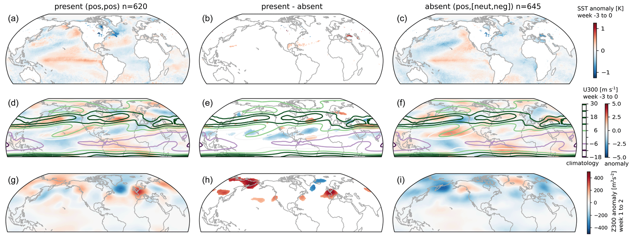
Figure 7 Modulation of the teleconnection when the west Pacific dipole in weeks −3 to 0 is in its positive phase. (a, d, g) samples with positive two-metre temperature (t2m) response in weeks 3 to 6, meaning a positive phase teleconnection (n=620). (c, f, i) samples resulting in a neutral or negative t2m response, meaning an absence of the teleconnection (n=645). (b, e, h) difference between panels in the left and right column. Values found to not exceed the difference as expected by random chance are masked (α=0.1, more detail in Sect. 5). (a, b, c) composite anomalies of sea surface temperature (SST) in weeks −3 to 0. (d, e, f) composite u₃₀₀ anomalies in weeks −3 to 0. Contour-overlay shows the summertime climatological u₃₀₀ value. (g, h, i) composite z₃₀₀ anomalies in weeks 1 to 2. Composites are extracted from the period 1980–2021 (climate normal also defined from 1980 to 2021).

7 Discussion and conclusion

In this study we have defined a WPD index that captures the strength of a dipole SST pattern in the western Pacific. The index captures a pattern of opposing SST anomalies in the central-to-west equatorial Pacific and the Western North Pacific region, i.e. a dipole with both equatorial and meridional orientation, which was shown to relate to changing patterns of deep convection and large-scale SST changes across the Pacific. Specifically, the WPD targets those heating patterns that excite QSRW, which potentially affect west and central Europe more than two weeks later. Such teleconnections are known mechanisms for sub-seasonal predictability. Cross-correlations make it clear that the emphasis of the WPD is different than, but still relates to, well-known Pacific modes (Fig. 3b, c). In particular, the positive and negative WPD phases in summer coincide with the strengthening of ENSO (Fig. 6).

A prominent result of this study is that negative WPD phases have become more frequent over recent decades. In this phase, convection over the Maritime continent and western north Pacific is enhanced, and that over the central Equatorial Pacific suppressed. Its increased occurrence reflects a long-term shift in the Pacific “background state” towards stronger zonal and meridional SST gradients, as a consequence of the west Pacific warming relative to the central tropical Pacific. This west Pacific warming mode is thought to be a response to anthropogenic forcing, and to strengthen the Walker circulation (Funk and Hoell, 2015; Funk et al., 2018).

Coinciding with the long-term SST changes we find that the WPD phase during weeks −3 to 0 becomes an important predictor for the European t2m response in weeks 3 to 6 (Fig. 4b) (also van Straaten et al., 2023). We diagnose that this summertime Pacific to Euro-Atlantic teleconnection emerged after 1980, which agrees with other studies (O'Reilly et al., 2019; Sun et al., 2022). We should however be cautious about concluding that the teleconnection was absent before 1980, as it can also relate to data quality, which improved with the advent of satellite observations (Hersbach et al., 2020). Nonetheless, we show that for the period 1980 to 2021 connectivity is significant, and that the teleconnection pathway can be well understood. Following the heating anomalies, a QSRW develops in weeks 1 to 2 and consists of known centres of action. Characteristic is the centre in the north-west US, south of Greenland and west of the British Isles (Fig. 5h) (Wulff et al., 2017; O’Reilly et al., 2018; Vijverberg and Coumou, 2022). The QSRW then extends further east, with large anomalies over our west and central European target region, and anomalies with an opposing sign over eastern Europe and Russia (an opposition also known from Behera et al., 2013; Lee et al., 2017).

The emergence of a significant teleconnection in recent decades provides a lens through which recent summer circulation changes over Europe can be interpreted. This is relevant because warming trends are the consequence of multiple factors such as direct forcing by greenhouse gases and aerosols (Dong et al., 2017), but also circulation changes (Deser et al., 2016; Faranda et al., 2023). The changes diagnosed in this study are an increased occurrence of negative WPD and a reduced occurrence of positive WPD, each with a respective QSRW response. The increased frequency of the negative WPD phase (Fig. 4a), would, according to its corresponding QSRW, induce a warming in eastern Europe and Russia (Fig. 5m). Indeed, high pressure has become more prevalent in this region (Lee et al., 2017; Kim and Lee, 2022; Teng et al., 2022), associated with a very strong increase in heat waves (Rousi et al., 2022), with average summer t2m increasing more than in our western European target region (Teng et al., 2022).

The warming of western European average summer t2m has been less severe, though still highly significant (Christidis et al., 2015; Gutiérrez et al., 2021). A precise quantification of the contribution from changes in WPD to this trend is beyond the scope of this study (and is also hindered by the methodological necessity to isolate the sub-seasonal teleconnection from the trend by using 21-year rolling-window distributions of t2m, see Sect. 4). But relative to the trend, two things can be said. First, during the time that negative WPD has roughly doubled in frequency (Fig. 8a), it has remained consistently related to the cold western European t2m tercile (Fig. 8b). This means that western European warming is likely caused by other factors.

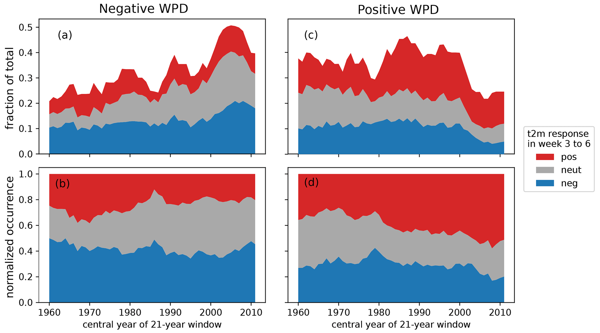
Figure 8 Prevalence of negative and positive West Pacific Dipole (WPD) phases over time (WPD index in weeks −3 to 0), as coloured by the resulting western European two-metre temperature (t2m) response in weeks 3 to 6. (a, c) presented as a fraction of the total number of samples within each 21-year rolling window. (b, d) presented as a fraction of the WPD phase itself, meaning normalized by the total prevalence of negative WPD (b) and positive WPD (d). Like in Fig. 4, tercile thresholds for WPD are determined over the entire dataset from 1950 to 2021, and tercile thresholds for t2m are re-computed in each window.

Second, one of these factors could be positive WPD. Although positive WPD reduced in frequency (Fig. 8c), we have seen that its corresponding QSRW is potentially modulated by the situation in the Atlantic (Sect. 6). A combination of an SST tripole and a strong and narrow jet in the north Atlantic allows the QSRW to reach western Europe. Prominent in this modulation are the relatively cold SSTs south of Greenland (agreeing with Fuentes-Franco et al., 2022). Such relatively cold SSTs have become prevalent since the 1980s (Chemke et al., 2020), just like the associated low pressure west of the British Isles (Faranda et al., 2023). This implies that although the total count of positive WPD phases decreases, those that do occur are more likely to generate a QSRW that reaches western Europe and results in warm t2m states there (Fig. 8d).

We suggest that the interplay between long-term Pacific changes and long-term north Atlantic changes might be researched further, particularly because cold north Atlantic SSTs can become more prevalent if Atlantic meridional overturning circulation slows down. Climate model experiments suggest that such slowdown might follow from further anthropogenic forcing and induce changes in summertime Euro-Atlantic circulation (Haarsma et al., 2015; Rousi et al., 2021). Relevant for the interplay are also long-term changes that potentially affect jet stream strength, like Arctic amplification and aerosols (Coumou et al., 2018; Dong et al., 2022).

Research into the Pacific–Atlantic interplay should probably not be conducted with numerical climate models only. Our analysis namely emphasized features that climate models have difficulty capturing. One is the strengthening of zonal gradients in Pacific SST, which we detected as the increase of negative WPD phases. We know that climate models are unable to reproduce the observed strengthening, and simulate a weakening instead (Funk and Hoell, 2015; Wills et al., 2022; Seager et al., 2022; Lee et al., 2022). It is worrying that even with prescribed SSTs, climate models fail to reproduce the associated dynamical response: an increased prevalence of high pressure over western and eastern Europe (Boe et al., 2020). It thus appears that climate models do not represent the detected QSRWs well. A similar failure to represent the teleconnection pathway happens in the ECMWF model, despite being initialized with observed SSTs (van Straaten et al., 2023).

Resolving these issues is challenging because the shortcomings of climate models force us to use observations or reanalysis products. These are of limited length, with few independent samples as a result. It is also challenging because a full theoretical understanding of QSRWs on different space- and timescales does not exist (White et al., 2022). We hope that the targeted WPD index provides future diagnostic studies with a starting point. An improved representation of the Pacific-to-Europe connection in weather and climate models has a lot to offer. One is a better projection of European summer extremes (van Oldenborgh et al., 2022). The other is a conditional opportunity to forecast European summer circulation more than two weeks in advance (Mariotti et al., 2020; van Straaten et al., 2023).

Appendix A: Optimality of time- and space scales

The teleconnection diagnostics presented in this study are based on certain chosen timescales. In particular, we relate four-week average SST anomalies (in the form of the WPD index) to four-week western European t2m anomalies, across a lead time gap of two weeks. In an earlier study, this configuration of lead time and aggregation period displayed some sub-seasonal predictability of European summertime t2m (van Straaten et al., 2022). Here we explore the position of these chosen timescales among alternatives. The black cross in Fig. A1a represents the current study, within a matrix of alternative averaging timescales (y axis) and lead time gaps (x axis). Figure A1b presents the values obtained when measuring concurrent association between WPD and western European t2m, without a lead time gap. For the concurrent, seasonal configuration (averaging a timescale of roughly 12 weeks), relatively strong association values are found (top in Fig. A1b). This is the approach that most earlier studies on the summertime Pacific to Europe connection take (Ting, 1994; Ding et al., 2011; Behera et al., 2013; O’Reilly et al., 2018). However, an equally strong or even stronger association is found for the shorter averaging timescale of 8 to 4 weeks, in which case the strongest link is not found concurrently, but at a lag of zero to one week between the end of the WPD period and the start of the t2m period (Fig. A1a). That a certain separation can be optimal is even clearer when we follow the correlation values horizontally along the two-week aggregation (Fig. A1a, second row from the bottom). These values peak at lags of 2 and 3 weeks, which corresponds to the finding that Rossby waves from tropics need time to fully establish in the mid-latitudes (e.g. Branstator, 2014). This leads us to conclude that although the Pacific to Europe teleconnection will show up in concurrent seasonal aggregates, it is quantitatively stronger in a non-concurrent framework, and thus has the character of a lagged sub-seasonal connection.

Figure A1 (a) Pearson correlation between West Pacific Dipole (WPD) and detrended western European two-metre temperature (t2m) at different lags and levels of temporal averaging (averaging applied equally to both WPD and t2m). Lag is defined as the number of intervening weeks (after the end of WPD and before the start of the t2m response). The black cross highlights the original lag and level of temporal averaging chosen in this study. The black square highlights the combinations presented in Figs. A2 and A3. Correlation is computed using data from 1980–2021. (b) Correlation obtained when WPD and t2m are fully overlapping (i.e. concurrent).

For the subset of the alternative temporal configurations highlighted by the black square in Fig. A1a, we compute correlation maps similar to those in Fig. 2b (we only investigate a subset because the computational cost is high). Figure A3 illustrates which cells remain robustly correlated within all five of the cross-validation folds in the data from 1950–2021. The original configuration of this study is displayed in Fig. A3c with the red title. One sees that the patterns shift when alternative timescales and lead time gaps are chosen. For instance, the cluster of cells extending from component 1 along the equator to the northern coast of Papua New Guinea (e.g. Fig. A3c, d) disappears on the shortest averaging timescale (Fig. A3i–k). Also influential is whether the cross-validation is performed on only the decades after 1980 (Fig. A2). In this case the equatorial extension is completely absent. Overall, we see that the component 1 and 2 boxes capture those parts of the patterns that appear in the majority of the configurations.

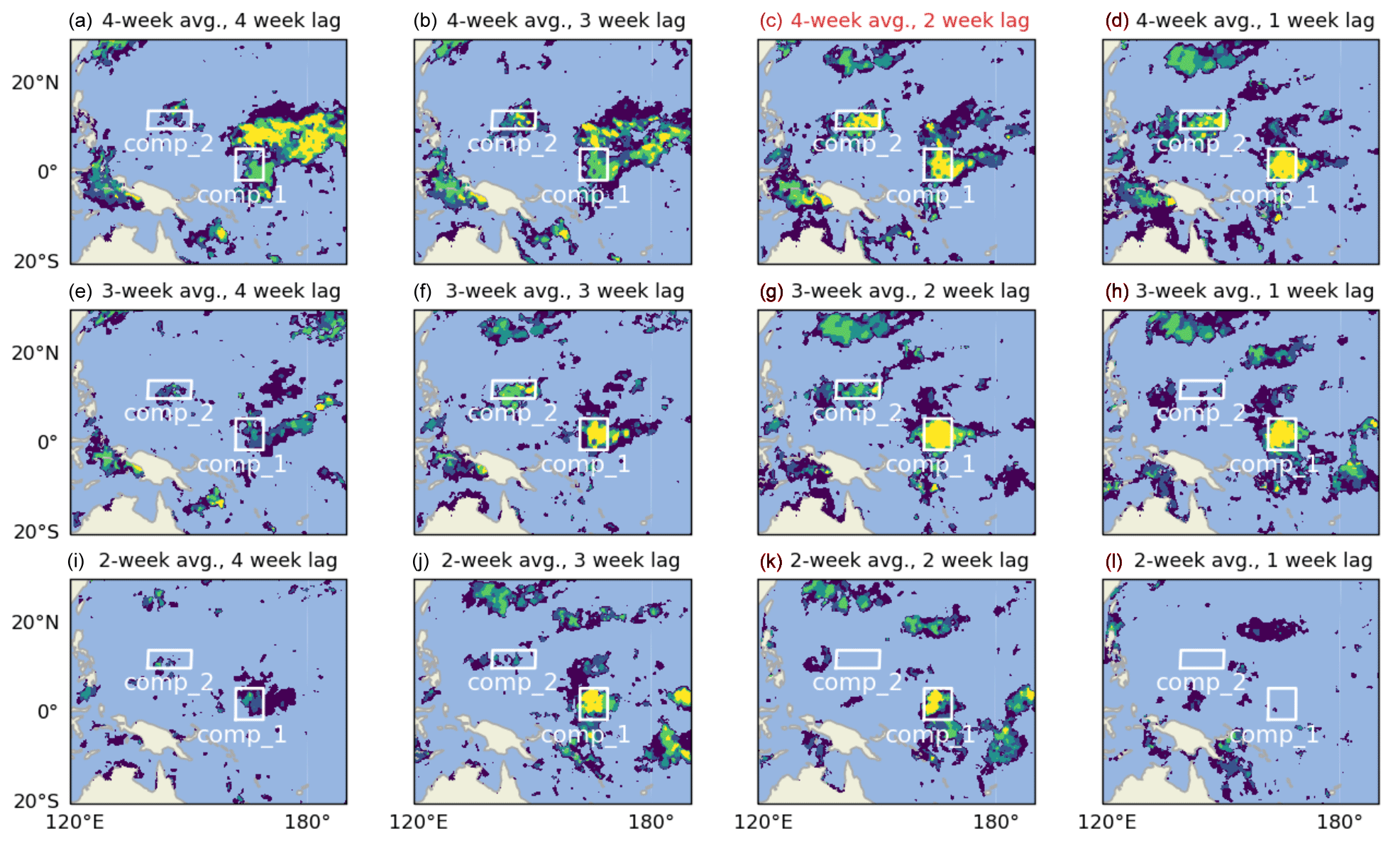
Figure A2 As Fig. 2b, but with partial correlation computed using reanalysis data from 1980 to 2021 (5-fold cross validation). Panels illustrate different combinations of lags and time aggregation applied to the SST anomalies and west/central European two-metre temperature (t2m). Temporal aggregation (rows) is applied to West Pacific Dipole (WPD) and t2m response equally. Lag (columns) is defined as the number of weeks after the end of WPD and before the start of the t2m response. Panel c shows the pattern under the original temporal aggregation and lag chosen in this study.

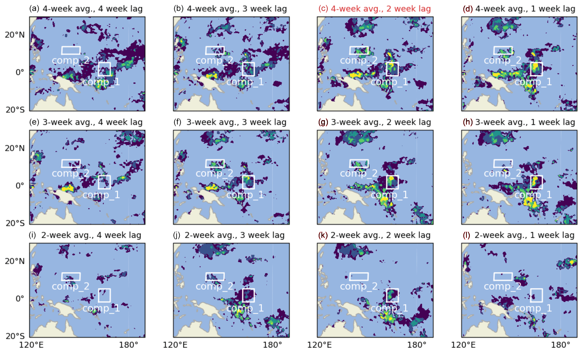
Figure A3 As Fig. A2, but with partial correlation computed using reanalysis data from 1950 to 2021 (5-fold cross validation). (c) shows the pattern under the original temporal aggregation and lag chosen in this study (in combination with using the full 1950–2021 data; it is therefore an exact copy of the map in Fig. 2b).