the Creative Commons Attribution 4.0 License.
the Creative Commons Attribution 4.0 License.
 | 28 Feb 2024
European summer weather linked to North Atlantic freshwater anomalies in preceding years
Marilena Oltmanns
N. Penny Holliday
James Screen
Ben I. Moat
Simon A. Josey
D. Gwyn Evans
Sheldon Bacon
Amplified Arctic ice loss in recent decades has been linked to the increased occurrence of extreme mid-latitude weather. The underlying mechanisms remain elusive, however. One potential link occurs through the ocean as the loss of sea ice and glacial ice leads to increased freshwater fluxes into the ocean. Thus, in this study, we examine the link between North Atlantic freshwater anomalies and European summer weather. Combining a comprehensive set of observational products, we show that stronger freshwater anomalies are associated with a sharper sea surface temperature front between the subpolar and the subtropical North Atlantic in winter, an increased atmospheric instability above the sea surface temperature front, and a large-scale atmospheric circulation that induces a northward shift in the North Atlantic Current, strengthening the sea surface temperature front. In the following summer, the lower-tropospheric winds are deflected northward along the enhanced sea surface temperature front and the European coastline, forming part of a large-scale atmospheric circulation anomaly that is associated with warmer and drier weather over Europe. The identified statistical links are significant on timescales from years to decades and indicate an enhanced predictability of European summer weather at least a winter in advance, with the exact regions and amplitudes of the warm and dry weather anomalies over Europe being sensitive to the location, strength, and extent of North Atlantic freshwater anomalies in the preceding winter.
- Article
(13004 KB) - Full-text XML
-
Supplement
(5282 KB) - BibTeX
- EndNote


Arctic near-surface temperature is currently warming twice as fast as the global average (Cohen et al., 2019), which manifests itself in an average sea ice volume loss of km3 per decade, based on the period 1979 to 2018 (Kumar et al., 2020). Similarly large losses are observed for land ice, particularly from the Greenland ice sheet, amounting to km3 per decade, based on the period 2003 to 2012 (Khan et al., 2015). Earlier studies noticed statistical links between an amplified sea ice loss at high latitudes and an increased occurrence of weather extremes at mid-latitudes (Francis and Vavrus, 2012; Tang et al., 2014; Screen and Simmonds, 2013; Cohen et al., 2014). However, the robustness of these links has been questioned, and the underlying mechanisms are poorly understood (Barnes, 2013; Overland et al., 2015; Blackport and Screen, 2020).
One potential connection occurs through the ocean. Specifically, the loss of sea ice and glacial ice in the Arctic and sub-Arctic regions constitutes a source of freshwater for the North Atlantic (Bamber et al., 2018; Carmack et al., 2016). Large North Atlantic freshwater anomalies, moreover, were found to give rise to cold surface anomalies and the development of storms in the subpolar region in winter (Oltmanns et al., 2020). In turn, cold anomalies in the subpolar region in winter were found to precede heat waves over Europe in the subsequent summer (Duchez et al., 2016; Mecking et al., 2019). The heat waves were attributed to a stationary jet stream over the North Atlantic (Duchez et al., 2016) and were successfully reproduced in model simulations initialized with the cold anomaly (Mecking et al., 2019). Thus, by triggering cold anomalies in winter, increased surface freshening could initiate a deterministic chain of events that first leads to cold anomalies and storms in winter and then heat waves in the subsequent summer.
While earlier studies support individual connections between the North Atlantic sea surface temperature (SST) and the jet stream (Woollings et al., 2010) or between shifts in the jet stream and European heat waves (Dong et al., 2013; Gervais et al., 2020), the role of freshwater in initiating this causal chain is unclear. Yet, given that the Arctic and sub-Arctic regions are expected to continue to warm and release freshwater from melting sea ice and glacial ice into the North Atlantic, it is critical to understand how the resulting feedbacks could affect weather in Europe.
The gap in our knowledge around the potential influences of North Atlantic freshwater anomalies on European summer weather arises from the difficulty in simulating salinity. Freshwater enters the subpolar region through narrow boundary currents and mesoscale eddies requiring ocean models with a fine grid spacing of ∘ (Marzocchi et al., 2015; Böning et al., 2016; Müller et al., 2019). Most current coupled global climate models have a coarser grid spacing, giving rise to salinity biases (Mecking et al., 2017; Menary et al., 2015; Wu et al., 2018). From an observational perspective, estimating freshwater variations is also difficult. In situ observations of sea surface salinity mostly stem from Argo floats which cannot fully capture the large spatial variability at high temporal resolution. Moreover, satellite observations of sea surface salinity are associated with large uncertainties and only available since 2009 (Bao et al., 2019; Xie et al., 2019).
Given the limitations associated with currently available model and observational products of sea surface salinity, we use a new approach to estimate freshwater variations, taking advantage of a dynamical constraint of the sea surface salinity on the SST. In the subpolar region in autumn and winter, the air is colder than the ocean surface. Thus, the surface water is cooled by the atmosphere, becomes denser, and sinks. Enhanced surface freshening reduces the surface density and requires additional cooling before the surface water is dense enough to sink. This constraint of freshwater on the surface cooling can be used to infer its variability using a mass balance analysis (Oltmanns et al., 2020).
In the following, we describe the involved data products (Sect. 2). We then explain the approach to estimate freshwater variability from a surface mass balance (Sect. 3). In Sect. 4, we examine the ocean–atmosphere evolution associated with freshwater anomalies and assess their links with European summer weather based on statistical analyses (Sect. 4). We conclude by discussing the dynamical role of freshwater anomalies in the identified ocean–atmosphere evolution and the implications for predictability (Sect. 5).
First, we describe the observational products involved in this study and describe any processing steps. Since the analyses are based on statistical methods, a high data quality is important. Thus, we focussed on the period since 1979, motivated by the increased data quality associated with the onset of satellite observations in 1979.
2.1 Datasets
The analysis of ocean variability includes a merged SST product consisting of Hadley Centre HadISST1 data (Rayner et al., 2003; Hurrell et al., 2008) and optimal interpolated, remote-sensing-based SST data from NOAA (Reynolds et al., 2002). The merged Hadley–NOAA data product has a monthly temporal resolution, has a spatial resolution, and is available at https://gdex.ucar.edu/dataset/158_asphilli.html (last access: 16 April 2023).
To assess changes in surface currents, we further used absolute dynamic topography data since 1993, derived from altimetry (Le Traon et al., 1998). Absolute dynamic topography represents the sea level anomaly with respect to the geoid and thus the stream function of the geostrophic surface flow. The monthly, gridded, absolute dynamic topography dataset has a spatial resolution of and is distributed by the Copernicus Marine Environment Monitoring Service (2023, https://doi.org/10.48670/moi-00148). Geostrophic surface velocities were calculated from the absolute dynamic topography using and , where ug and vg are the zonal and meridional geostrophic velocities, η is the absolute dynamic topography, g is the gravitational acceleration, f is the Coriolis parameter, RE is the Earth's radius, and θ and ϕ are the latitude and longitude respectively.
Moreover, to compare freshwater anomalies, estimated from the surface mass balance analysis, with in situ observations from the subpolar North Atlantic, we included a hydrographic, mixed layer database. The dataset provides mixed layer depths, mixed layer salinities, and mixed layer temperatures derived from Argo float profiles (Holte et al., 2017). It is freely available at http://mixedlayer.ucsd.edu (last access: 11 January 2018).
The ocean data are complemented by monthly output from the ERA5 atmospheric reanalysis model from the European Centre for Medium-Range Weather Forecasts since 1979 (Hersbach et al., 2018). In addition to the standard variables, we estimated the maximum Eady growth rate using monthly mean output from ERA5 to qualitatively assess the baroclinic instability in the lower troposphere over increased meridional SST gradients. Following earlier studies (Lindzen and Farrell, 1980; Dierer and Schluenzen, 2005), the maximum Eady growth rate in the 1000 to 750 hPa layer was calculated as , where f is again the Coriolis frequency, u is the zonal wind, z is the height, N os the Brunt–Väisälä frequency, and the subscripts refer to the associated pressure levels.
A key parameter used to derive freshwater indices is the mean North Atlantic Oscillation (NAO), obtained from the National Oceanic and Atmospheric Administration (NOAA) Climate Prediction Center. The NAO index was calculated using rotated principal component analysis, applied to the monthly standardized 500 hPa geopotential height anomalies between 20 and 90∘ N (Barnston and Livezey, 1987). It corresponds to the dominant mode of variability in the Northern Hemisphere. A detailed derivation can be found at https://www.cpc.ncep.noaa.gov/products/precip/CWlink/pna/nao.shtml (last access: 9 March 2023).
Lastly, we included data from the Greenland climate model MAR to assess potential causes of freshwater anomalies. We used version 3.12, run at a resolution of 20 km forced by the ERA5 reanalysis (Fettweis et al., 2017) and distributed by the Laboratory of Climatology at the University of Liège. For the purpose of this study, we considered the runoff over the full ice sheet from 1950 through to the end of 2022 at monthly resolution. The dataset is available at ftp://ftp.climato.be/fettweis/MARv3.12 (last access: 7 April 2023).
2.2 Preprocessing
Over the investigated period, the climate has been characterized by increasing greenhouse gas concentrations, leading to enhanced surface warming (Lashof and Ahuja, 1990). Over the last 2 decades, moreover, the freshening has also been increasing (Tesdal et al., 2018), particularly because of increased runoff and melting from Greenland (Bamber et al., 2012, 2018). Thus, the surface warming resulting from increased greenhouse gases could be superimposed on potential surface cooling or warming signals resulting from changes in the ocean or atmospheric circulations associated with increased North Atlantic surface freshening. This superposition could distort the interpretation of the statistical analyses when assessing the specific influences of changes in the ocean and atmospheric circulations associated with increased North Atlantic freshening.
Considering that the freshening trend is an important part of the signal we are investigating, removing trends at each location (or grid point) would remove an important part of a signal that we are interested in. Thus, to reduce the influence of increasing greenhouse gas concentrations on European air temperatures, we subtract regionally averaged trends from the air temperature. The method of subtracting regionally averaged trends is motivated by the observation that greenhouse gases are distributed comparatively uniformly in the atmosphere (Reuter et al., 2020), whereas the observed surface warming exhibits large regional differences (Simmons, 2022). These regional differences in surface warming result from changes in the ocean and atmospheric circulations, which are redistributing the excess heat. Since, in this study, we are specifically interested in these dynamic processes associated with changes in the ocean and atmospheric circulations, we are subtracting a spatially uniform warming trend associated with increasing greenhouse gases.
We tested different regions and found that the results are not sensitive to the exact area that is used for the averaging, as long as it is sufficiently large. Here, we averaged over the main area of investigation from 25 to 65∘ N and from 60∘ W to 60∘ E, resulting in an average trend of ∼0.04 ∘C yr−1 in the 2 m air temperature from ERA5. Extending the region in any direction does not appreciably change this trend, nor the subsequent results, consistent with the assumption that the direct warming trend that is solely due to increasing greenhouse gases is distributed relatively uniformly.
While the summer air temperature is strongly affected by a spatially uniform warming trend, the other variables exhibit no or only minor trends after they have been averaged over a large area. Thus, after removing the trend in the air temperature prior to the analyses, we obtain a signal that is dynamically consistent across all investigated variables. If, on the other hand, we do not remove the trend in the air temperature, we still obtain the same patterns throughout the results, but there would be a large-scale, uniform warming signal superimposed over the full domain.
We did not apply any other averaging, smoothing, filtering, or further preprocessing steps to the datasets.
The objective of this study is to investigate feedbacks initiated by freshwater anomalies. However, high-quality global salinity measurements have only been routinely available since 2002 and mostly in the open ocean from Argo floats. Moreover, satellite observations of the sea surface salinity are of relatively low accuracy and only available since 2009 (Bao et al., 2019; Xie et al., 2019). Considering the limitations associated with currently available salinity products, we use a surface mass balance analysis to estimate the variability in freshwater.
3.1 Mass balance
The mass budget for the surface mixed layer in the subpolar region in winter can be expressed as
where ρ is the mixed layer density, h is the mixed layer depth, η is the surface elevation above the geoid (which is equivalent to the absolute dynamic topography), g is the gravitational acceleration, B is the buoyancy flux through the surface, and u corresponds to the velocity vector (Gill, 1982; Griffies and Greatbatch, 2012). The term represents the convergence of mass, which we separate into an active component A and a passive component E. The passive component is defined as the entrainment of mass into the mixed layer that results from mixed layer deepening as the mixed layer density increases. The active component results from externally forced, horizontal, and vertical mass fluxes, such as wind-driven Ekman transports and upwelling. The passive component can only change the mixed layer depth but not its density, while the active component does change the mixed layer density.
Next, we assume that the density is homogeneous in the mixed layer and that η in winter is much smaller than the mixed layer depth h. After integrating Eq. (1) from summer to winter and neglecting the contribution of the surface elevation η relative to the mixed layer depth on the lefthand side of Eq. (1), we thus obtain
where h0 and ρ0 represent a mixed layer depth and density at the end of the summer (for instance in September), h and ρ refer to the depth and density in winter (January to March), and Δt is the corresponding integration interval from summer to winter.
While the climatological mean mixed layer density increases during the winter, the mixed layer deepens. Thus, before the winter, the mixed layer is several tens of metres deep, while during the winter, it reaches several hundred metres. Since the density anomaly in the initial shallow mixed layer becomes distributed over a much larger depth range, the first term on the righthand side is negligible compared to the other terms. Any density anomalies beneath the initial, shallow mixed layer are still included in E. Equation (2) thus simplifies to
We further separate each term into a mean and an anomaly n, with n referring to the nth winter of an arbitrary subset of N winters and the mean representing the mean over these winters. Since we have defined E as a passive component that can only change the mixed layer depth, not its density, we can write it as . Moreover, assuming that the mean state is in balance, we subtract the mean values from Eq. (3), resulting in
where the terms involving hn cancel each other out.
Lastly, we express the density as a function of temperature and salinity by considering variations in the density around a reference state, which we choose to be the mean over the N selected winters. Since local density variations due to pressure are several orders of magnitude smaller than those due to changes in salinity and temperature (Talley, 2011), we only consider temperature and salinity variations: , where T is the temperature, S is the salinity, and α and β are the thermal and haline expansion coefficients. Plugging this expression into Eq. (4), we obtain
The objective of the following analysis is to find conditions in which the density anomalies associated with temperature anomalies are much larger than the effect of potential, active drivers of density anomalies on the righthand side of Eq. (5): . Under these conditions, the temperature and salinity anomalies must compensate each other in their influence on density, allowing us to estimate the salinity anomalies from the associated temperature anomalies: βSn≈αTn.
The idea that such conditions exist is motivated by the observation that salinity changes not only are a response to surface fluxes and entrainment but can, in turn, constrain the drivers of density anomalies. Large freshwater anomalies in winter can impede convection and entrainment and thus limit the oceanic heat release to the atmosphere (B). At the same time, a stronger surface cooling is required to mix freshwater down, influencing the mixed layer temperature T. Considering the competing influences of salinity and temperature on stratification, the conditions in which freshwater may impact the temperature can only occur in autumn and winter, when surface water is cooled by the atmosphere, becomes denser, and sinks. In summer, the temperature and salinity do not compete in their influence on stratification and thus do not constrain each other.
To exploit this constraint of salinity on temperature and identify these potential conditions, we assume that the surface mixed layer in winter is relatively well mixed, so we can approximate the mixed layer temperature T with the SST. We then search for potential freshwater indices that exhibit a strong linear relationship with subpolar SST anomalies, regress Eq. (5) onto these indices, and compare the magnitude and spatial characteristics of the resulting terms. If enhanced surface freshening substantially affected the SST, we expect the terms An and Bn to drop out of Eq. (5) after the regression. In essence, the indices serve as filters that help us to identify conditions in which freshwater anomalies have been sufficiently large to influence the heat exchange between the ocean and the atmosphere, either within the subpolar region or before entering it. Later (in Sect. 4.5), we will further assess if these conditions in which the air–sea heat exchange and, in turn, the SST have been affected by freshwater anomalies hold generally over the North Atlantic or only for selected indices.
3.2 Derivation of freshwater indices
The challenge in detecting the conditions in which freshwater anomalies may have affected the SST consists in the complexity of SST and freshwater variability in the subpolar region. In theory, changes in surface freshwater can be influenced by river runoff, sea ice and glacial melting, evaporation and precipitation, mixing, and ocean currents. Considering that multiple factors can contribute to freshwater variations over a range of timescales and spatial scales, it may not be possible to reduce the complexity of freshwater variability in space and time into a single, one-dimensional index.
To overcome this challenge, we construct indices over subsets of years that allow us to closely constrain the variability in the SST over the selected subset. Thus, this approach is different to traditional methods in which the dynamical mechanisms are known a priori, and statistical methods are used to assess the significance of these mechanisms. Here, we first select indices with a strong and significant statistical relationship with the SST and then look for potential freshening mechanisms that can explain the relationship, assuming that these mechanisms exist but may be masked by other drivers.
As a first, educated guess to identify suitable freshwater indices, we start with the NAO index in summer (Fig. 1a), motivated by its dynamical links to freshwater. On the one hand, a more negative NAO phase in summer has been associated with enhanced runoff and melting over Greenland (Hanna et al., 2013, 2021), which is a source of freshwater to the North Atlantic (Bamber et al., 2018; Dukhovskoy et al., 2019). On the other hand, a more positive NAO phase has been associated with an intensified subpolar gyre circulation, leading to enhanced freshwater imports into the subpolar region (Häkkinen et al., 2011a, 2013; Holliday et al., 2020). Yet, even if the freshening occurs in summer (when melting and runoff are strongest), the effect of the freshwater on the SST would only become visible in autumn and winter (when the freshwater impedes the sinking of surface water). Thus, we focus on the SST in winter to infer the occurrence of freshwater anomalies.
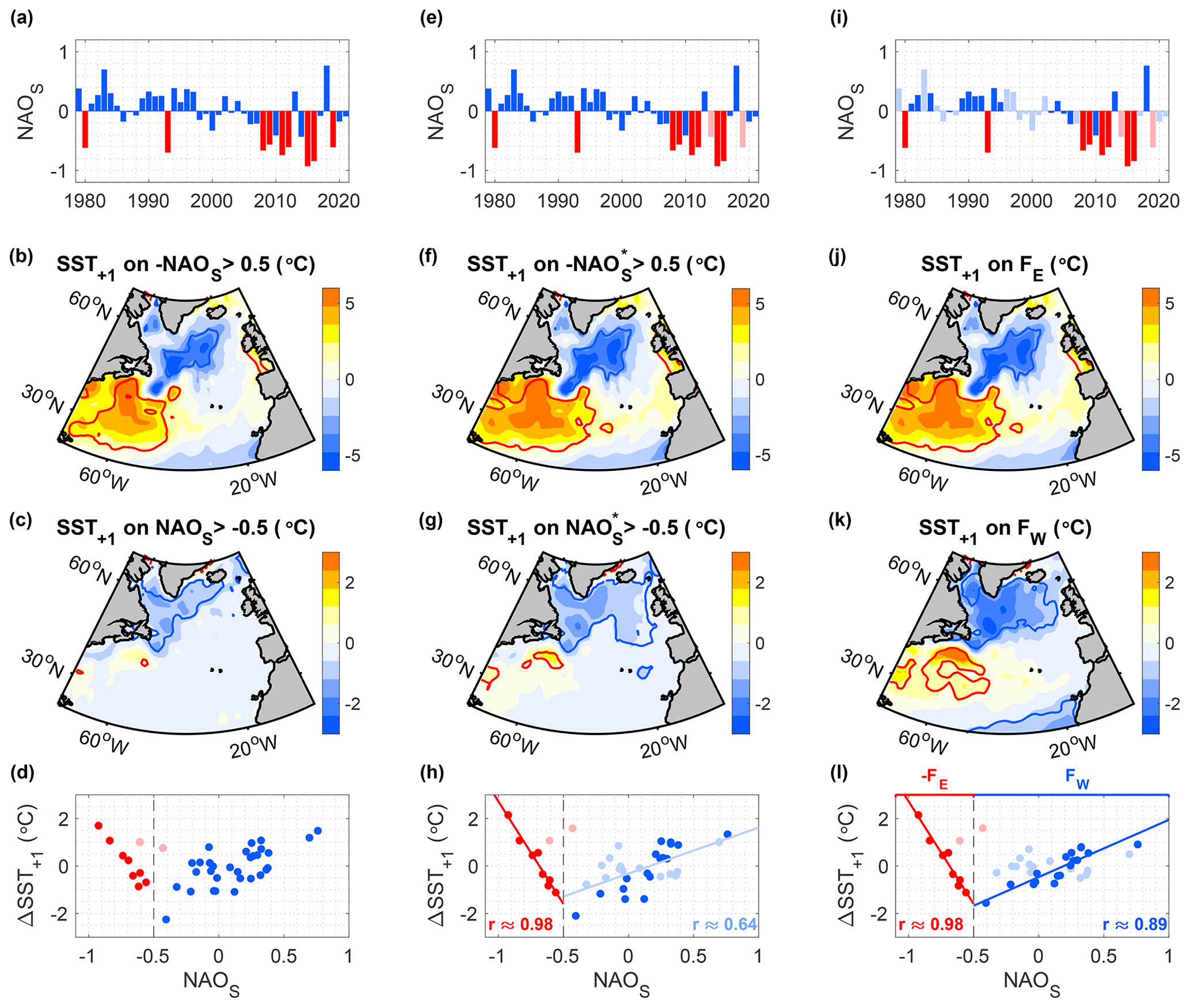
Figure 1(a, e, i) Variability in the NAO index in July and August (NAOS). The strong red coloured bars represent the NAO years used for the regressions in the second row (b, f, j), and the strong blue coloured bars represent the NAO years used for the regressions in the third row (c, g, k). Light coloured bars indicate the years that were removed in the course of the subsampling. (b, c) Regression of the SST in winter (January through to March) onto (b) in all years in which NAO and (c) NAOS in all years in which NAO. The SST anomalies correspond to the winter following the NAOS summers (indicated by the “+1” in the titles). (f, g) As in (b) and (c) but for NAO corresponding to NAOS without the two light red coloured outliers. (j, k) As in (b) and (c) but for the final two freshwater indices FE and FW (shown by the strong coloured years in i and l). Contours encompass regions that are significant at the 95 % confidence level. Please note the different colour scales. (d, h, l) Relationship between NAOS and the subsequent ΔSST in winter, where ΔSST represents the SST difference between the red subtropical and the blue subpolar 95 % confidence regions in the respective panels above (b, f, j) for the red years and (c, g, k) for the blue years, relative to the temporal means over each subset. Light coloured dots correspond to years that are rejected in the course of the subsampling. The final indices FE and FW are shown as strong coloured dots in (l).
Consistent with the existence of multiple possible drivers of freshwater and SST anomalies in winter, we obtain a qualitatively different relationship between the summer NAO index in July and August (NAOS) and the temperature difference between the subpolar and subtropical gyres in the subsequent winter below and above a threshold of in NAOS (Fig. 1a–d). Below the threshold of , there is a progressively larger SST difference between the northern subtropical region and the southern subpolar region for decreasing NAOS phases in the preceding summer (Fig. 1b). Above this threshold, there is a progressively larger SST difference for increasing NAOS phases in the preceding summer. Also, the associated cold, subpolar SST anomaly is weaker and displaced further to the northwest (Fig. 1c). The threshold of was initially identified using box regions for the subpolar and subtropical regions (for instance with latitudinal boundaries between 45 and 60∘ N for the subpolar region and between 30 and 45∘ N for the subtropical region), but the identified relationships are not sensitive to the exact region.
Next, we strengthen the identified relationships between the two NAO subsets (above and below −0.5) and the subsequent SST anomalies through subsampling. Specifically, if xi corresponds to the NAOS subset years and yi corresponds to the SST anomaly in the subsequent winter, we strive to derive a linear relationship , where a and b are constants and in which is high. The higher the magnitude of a is, the higher the magnitude of αT is on the lefthand side of Eq. (5) after regressing Eq. (5) onto the index. Thus, we aim to select NAO years for which the magnitude of the slope is large, where , and represents the (temporal) mean over the subset yi. At the same time, we strive to obtain a high correlation between the subset and the subsequent SST anomalies. Thus, we aim to select NAO years where (xi−x0)2 is large, since this increases the variance of the SST anomalies that can be explained by the index.
The values of xi included in each subset directly correspond to the respective NAOS values without scaling them, while the values of yi correspond to the observed SST difference between the subpolar and the subtropical gyres in any given year (ΔSST) rather than only the SST anomaly at a single location. Using the SST difference has the advantage that we filter out any spatially uniform, radiative warming signals due to increasing greenhouse gas concentration. In addition, we only average the SST over regions in which the SST anomalies are significant (Fig. 1b and c), allowing us to directly inspect the robustness of the correlations and ensure that they are not due to outliers or clusters. Thus, we identify two outliers, corresponding to the NAO summers in 2014 and 2019 (faint red years in Fig. 1d), which we exclude from the subsequent subsampling to obtain a faster convergence of the results. Individual inspection of both years showed that they were associated with pronounced cold, subpolar SST and freshwater anomalies. However, their relation to NAOS differed from those in the other years, precluding them from being included in the subsets.
Following the above objectives to maximize the slope and variance of the subsampled index, we select the N years where the term is highest. Here, the subscript i refers to all years in each subset, excluding the two outliers, and y is the associated, linear regression of yi on xi (Fig. 1e–h). Graphically, the subsampling is equivalent to increasing the slope of the regression line (the light blue line in Fig. 1h) while keeping a high variance. Thus, the method aims at increasing the statistical relationship between two variables for identifying dynamical links, based on the assumption that noise, and other mechanisms, can mask these links. Once a strong statistical connection has been established, the physical basis will be assessed by investigating the potential, underlying dynamical links.
There is a trade-off between the number of years N included in each subset and the resulting correlations between the NAO subset and subsequent SST pattern. Considering that the number of years is already low for the cold anomalies preceded by negative NAO summers, where NAOS is smaller than −0.5 (N=8), we do not apply any further subsampling (Fig. 1i and j). For the other subset (corresponding to the NAOS years higher than −0.5), we select N=17 years as a reasonable compromise for obtaining a high correlation while keeping a relatively large sample size (Fig. 1i and k). Thus, we achieve an increase in the correlation between the subsampled NAOS index and the resulting SST difference between the subpolar and subtropical region from ∼0.64 to ∼0.89, resulting in a low p value of (Fig. 1h and l).
In Sects. 4.5 and S2, we show that the results are not sensitive to the subsampling or the number of years included. However, having a close relationship between the index and the SST results in reduced uncertainties when estimating the associated freshwater anomalies. In addition, the high correlations help us to identify and assess potential dynamical links more clearly: freshwater indices that are only poorly correlated with freshwater are only of limited use when assessing links between freshwater and other ocean or atmospheric parameters. Since the indices will be used as a tool for representing freshwater anomalies, high correlations between the indices, the SST, and potential freshwater anomalies are a prerequisite, not a conclusion, and we make no assumptions on the suitability of both subsets outside the selected years.
Through the subsampling, we have derived two subsets with close, linear relationships with the SST difference between the subpolar and subtropical gyre (Fig. 1i–l). To distinguish the two subsets from each other, we name them according to the location of the associated cold SST anomalies. Since the maximum cold anomalies associated with are strongest over the southeastern subpolar region (Fig. 1j), we refer to the selected 8 years as FE index – shown by the clear red coloured bars in Fig. 1i. For the other subset, the maximum cold anomalies extend over the full subpolar gyre, including the western part (Fig. 1k). Thus, we refer to the selected 17 years as FW index – shown by the clear blue coloured bars in Fig. 1i. The corresponding years included in each index are additionally listed in Table A1. In the following analyses, we will examine the dynamical links of both indices to freshwater anomalies and the associated air–sea feedbacks.
Having selected two NAO subsets, we will first assess their suitability for representing freshwater anomalies. Thus, we evaluate the associated mass balance to estimate freshwater anomalies and examine their potential causes. We will then use the indices to investigate links between the estimated freshwater anomalies and the large-scale ocean and atmospheric conditions in winter and summer and test if the identified links hold generally by using an un-subsampled index. Lastly, we will assess the role of North Atlantic freshwater anomalies as a predictor for Europe's warmest summers by constructing composites of the 10 warmest relative to the 10 coldest summers between 1979 and 2022 and comparing the preceding freshwater anomalies.
4.1 Estimation of freshwater anomalies
Taking advantage of the strong relationships between the selected NAOS subsets and subsequent SST anomalies, we regress each term in Eq. (5) on the corresponding indices FE and FW. We then evaluate the surface mass balance over the subpolar cold SST anomaly regions within the regions enclosed by the 95 % confidence lines. In the following, we present the key analysis steps and results, while a detailed evaluation and comparison with in situ observations is provided in Sect. S1 in the Supplement.
To estimate the temperature term αTn, we again assume that the mixed layers are relatively homogenous and approximate the mixed layer temperature with the SST, averaged over the winter (January through to March). Even if the SST is slightly warmer or colder than the mixed layer temperature, the relationship between the mixed layer temperature and the mixed layer salinity will still remain the same as that between the SST and the sea surface salinity due to having a constant density profile in the mixed layer. To estimate the mean mixed layer depth hmean, moreover, we averaged the mean mixed layer depth, obtained from Argo floats (Holte et al., 2017), over the same regions and months as the SST, resulting in a mean mixed layer depth of ∼250 m for the FE subset and ∼280 m for the FW subset.
We further compute α and β using the Gibbs Seawater routines (Intergovernmental Oceanographic Commission, 2015), in accordance with the highest standards of current knowledge. Noting that the effects of salinity and pressure on α and β are small and only affect the second decimal place or less, we use nominal values of 35 g kg−1 and 10 db for the subpolar region in winter to compute α and β. The dependence of α and β on temperature is larger, however. For instance, α can vary from to ∘C−1 across the subpolar ocean surface. Thus, for an enhanced accuracy, we allow α and β to vary with the SST.
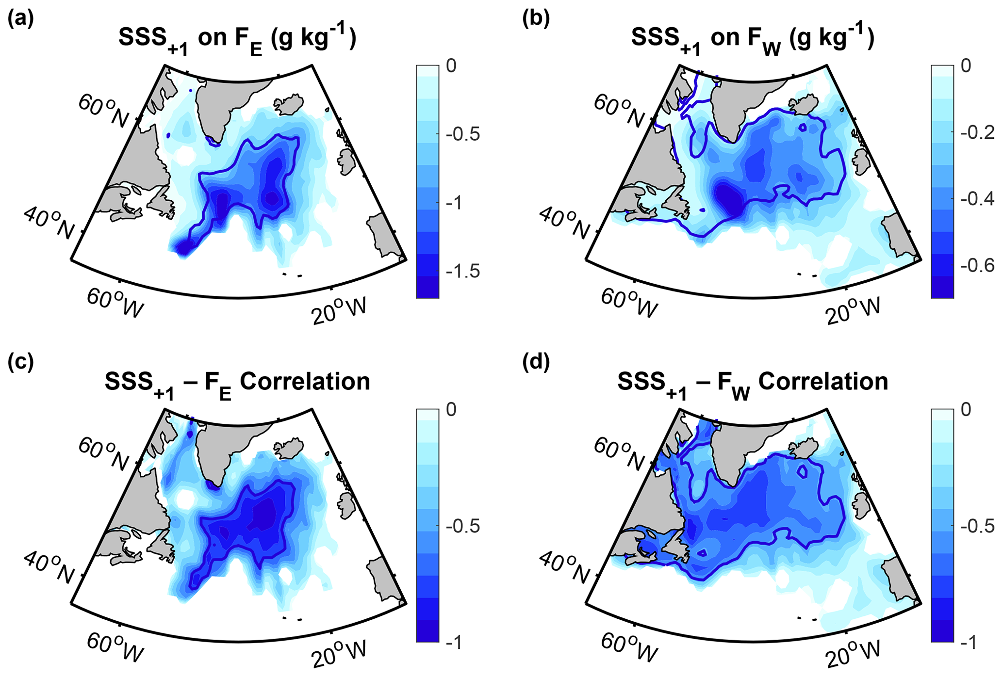
Figure 2(a, b) Regression of the sea surface salinity in winter (January through to March) on the two freshwater indices from the preceding summer (Fig. 1i). The contours delineate the regions that are significant at the 95 % confidence level. (c, d) Correlations between the sea surface salinity in winter and the freshwater indices from the preceding summer, with the thick contours delineating the regions that are significant at the 95 % confidence level, assessed by means of two-sided t tests. The underlying sea surface salinity variability has been estimated from the surface mass balance by assuming density compensation with the SST anomalies.
Next, we estimate the terms on the righthand side of Eq. (5). On the timescales and spatial scales considered, oceanic flows are predominantly in geostrophic balance, redistributing heat and freshwater. However, geostrophic flows cannot contribute to a net mass input. Over the open ocean, away from topographic boundaries, on interannual timescales, the winds and air–sea fluxes represent the largest energy sources that can result in vertical mixing or horizontal mass convergence (Ferrari and Wunsch, 2009; Wunsch and Ferrari, 2004). Other sources of energy include pressure loading by the atmosphere, geothermal heating, biological activity, and the tides, but we estimate them to be negligible over the investigated timescales and spatial scales. Thus, the terms on the righthand side of Eq. (5) are confined to the surface buoyancy fluxes, horizontal Ekman transports, and wind-driven vertical fluxes, all of which are estimated using the atmospheric reanalysis ERA5. Considering the nonlinearity within the individual terms of Eq. (5), we first evaluate each term before regressing it onto the indices.
After estimating the density anomalies associated with the cold anomalies and the buoyancy fluxes, the horizontal Ekman transports, and the vertical Ekman velocity and then regressing them onto the freshwater indices (Sect. S1), we find that, regardless of the exact region and mean mixed layer depth and regardless of which month is selected as the starting month of the integration, the density increase implied by the cold anomalies associated with FE and FW is always more than an order of magnitude larger than the density changes associated with An or Bn. Moreover, neither of these fluxes is significantly correlated with the subsets, and their spatial patterns are inconsistent with the obtained SST patterns, regardless of whether we include the full subpolar region where the SST anomaly is negative or only the region enclosed by the 95 % confidence lines or whether we start the integration in October or only consider the winter months of January to March.
With the buoyancy fluxes, vertical Ekman transports, and horizontal advection being negligible, we conclude that the density increase associated with the cold anomalies must be balanced by a density decrease associated with freshwater anomalies: αSSTE≈βSSSE, and αSSTW≈βSSSW, where SSS is the sea surface salinity and the subscripts refer to the anomalies obtained from the regressions onto the respective index. This result implies a close connection between freshwater and SST anomalies included in each subset. A demonstration of the connection between SSS and SST anomalies with hydrographic observations shows that, even in winters with the most intense air–sea fluxes, freshwater anomalies can still be inferred from the SST with reasonably small uncertainties (Sect. S1).
Using the obtained density compensation between SSS and SST anomalies, we estimate SSS anomalies from the two NAO subsets. Thus, we find that the maximum freshwater anomalies (or minimum SSS anomalies) associated with FE occur over the central subpolar region (corresponding to the southeastern subpolar gyre) and are spatially more confined than the maximum freshwater anomalies associated with FW (Fig. 2a and b). Moreover, the significant area of FW freshwater anomalies extends further eastward, westward, and northward compared to FE freshwater anomalies, and the anomalies have a smaller amplitude, consistent with the associated cold, subpolar SST anomalies (Fig. 1j and k).
Since the buoyancy fluxes represent the largest term on the righthand side of Eq. (5), they determine the uncertainty of the obtained salinity estimates, amounting to 4 % for the FE subset and 6 % for the FW subset. These uncertainties apply to the cold anomaly regions, enclosed by the 95 % lines. Uncertainties at each individual grid point can differ. Moreover, if the freshwater forcing is very large, the surface mass balance may underestimate the freshening because freshwater anomalies can (in theory) increase up to a salinity threshold of zero, while SST anomalies cannot drop below the air temperature. Still, we find that even during the strong observed freshwater anomalies in 2015 and 2016, the surface mass balance provided a good approximation (Sect. S1), suggesting that a potential underestimation is only small.
In addition to the low overall uncertainties of the SSS estimates, another implicit advantage of the selected NAO subsets FE and FW is that they are, by construction, highly correlated with the obtained freshwater estimates in the subsequent winter, with the magnitude of the correlations between the SSS anomalies and the freshwater indices exceeding 0.9 (Fig. 2c and d). The SSS correlations with the FE subset reach their highest magnitude over the southeastern subpolar gyre, while the highest magnitudes of the SSS correlations with FW occur over the central and northern subpolar region, covering an overall larger area, like the corresponding regressions. Considering the low uncertainties of the obtained freshwater estimates and their high correlations with the two NAO subsets, we conclude that both subsets represent suitable freshwater indices.
4.2 Causes of freshwater anomalies
Freshwater anomalies may result from enhanced sea ice or glacial melt, river runoff, surface fluxes (precipitation minus evaporation), and circulation changes. After investigating the surface fluxes from ERA5, glacial runoff from the Greenland climate model MAR, and the regional gyre circulation from altimetry, we find a significant anti-correlation between the summer NAO and runoff (Fig. 3a), pointing to runoff as a potential freshwater source for the FE freshwater anomalies since they are preceded by a strongly negative summer NAO. While other sources of meltwater, such as sea ice, may also contribute to enhanced freshening, the correlation between runoff and the summer atmospheric circulation is consistent with other studies evaluating individual links between the summer atmospheric forcing and glacial runoff (Hanna et al., 2013, 2021), as well as the resulting freshwater input into the North Atlantic (Bamber et al., 2018; Dukhovskoy et al., 2019).
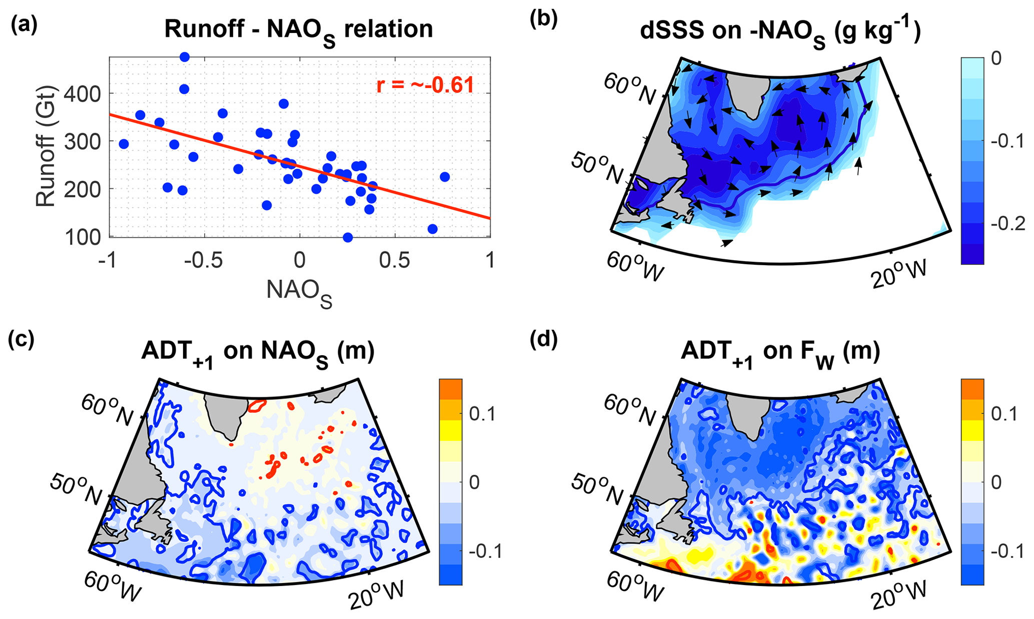
Figure 3(a) Relationship between the NAO in July and August (NAOS) and Greenland runoff integrated over the ice sheet from July to August. (b) Regression of the newly arriving, seasonal surface freshening between summer (August) and winter (January to March) onto from the preceding summer; dSSS corresponds to the SSS change from summer and winter, estimated using a mass balance analysis (Oltmanns et al., 2020). The arrows represent the mean geostrophic surface flow, obtained from the absolute dynamic topography, averaged from August to March (the freshening period). Multiplying the summer NAO by “−1” serves the purpose of using an index that is positively correlated with the surface freshening. (c, d) Regression of the absolute dynamic topography in winter (January to March) onto (c) NAOS and (d) FW from the preceding summer. Contours in (b)–(d) encompass regions that are significant at the 95 % confidence level.
With the majority of seasonal runoff arriving in the subpolar gyre during autumn (Fratantoni and McCartney, 2010; Schmidt and Send, 2007), the change in the surface salinity from summer (August) to winter (January to March) has previously been estimated by evaluating the mass balance of a shallow surface layer (Oltmanns et al., 2020). Thus, the summer NAO, multiplied by “−1” was identified as a suitable index for the seasonal freshwater that reaches the subpolar region between August and winter (Fig. 3b). The timing of the increased seasonal freshwater input associated with supports the role of seasonal runoff and melting for the FE freshwater anomalies. However, we point out that the relationship between the NAO index and runoff cannot explain differences in the freshwater anomalies within the FE subset. Instead, it explains the existence of the FE subset in the first place since runoff and increased surface melting are the only drivers of freshwater anomalies that are anti-correlated with the summer NAO.
While the full, un-subsampled summer NAO is a suitable indicator of runoff and the seasonal surface freshening from summer to winter, it is not necessarily correlated with absolute SSS anomalies in winter. Once a seasonal mixed layer is eroded, the SST and surface salinity are expected to be influenced by other factors, consistent with the nonlinear relationship between the summer NAO and subsequent winter SST anomalies (Fig. 1l).
Among the dominant drivers of deeper freshwater anomalies is the subpolar gyre circulation. Specifically, a stronger subpolar gyre circulation, particularly in the northwestern subpolar region, has been found to lead to enhanced inflow of fresh and cold polar water from the coastal Labrador Current into the subpolar gyre (Häkkinen and Rhines, 2009; Häkkinen et al., 2011a, 2013; Koul et al., 2020). Since the subpolar gyre circulation is, in turn, largely forced by the wind stress (Häkkinen et al., 2011b; Spall and Pickart, 2003), earlier studies have identified a significant link between a stronger wind stress curl over the subpolar North Atlantic and a reduced salinity in the subpolar gyre (Häkkinen and Rhines, 2009; Häkkinen et al., 2011a, 2013; Hátún et al., 2005; Holliday et al., 2020).
To assess the role of the wind stress curl and subpolar gyre circulation for the cold and fresh anomalies associated with higher summer NAO states, we inspect the associated absolute dynamic topography in winter. The full, un-subsampled summer NAO only displays a weak and mostly non-significant relationship with the geostrophic surface circulation in the southwest subpolar region (Fig. 3c). When using the subsampled summer NAO corresponding to the FW subset, however, the absolute dynamic topography north of 50∘ N in winter is significantly reduced, implying a more cyclonic and, hence, stronger subpolar gyre circulation in the northwest subpolar region (Fig. 3d). The strengthened relationship between the subsampled summer NAO and the subpolar gyre circulation thus supports the subsampling by providing a physical explanation for the freshwater anomalies associated with FW (Fig. 2b). For the rejected years (in the second step of the subsampling), the dependence of hydrographic anomalies on the subpolar gyre circulation still holds (Häkkinen et al., 2011a, 2013), but the NAO index is not a suitable indicator of this circulation.
While a detailed quantification of the freshwater budget is beyond the scope of this study, the proposed physical causes of the obtained freshwater estimates are supported by their spatial characteristics and intensities. FW freshwater anomalies are largest over the western subpolar region, where the subpolar gyre circulation is strongest and where the surface heat fluxes are largest, and can erode seasonal freshwater anomalies more easily. FE freshwater anomalies are largest over the southeastern part of the subpolar region where surface fluxes and the subpolar gyre circulation are weaker and where the mixed layer depths are shallower. We also examined the associated surface fluxes (precipitation minus evaporation) but found that they were too weak to account for freshwater anomalies. In autumn and winter, moreover, the surface freshwater fluxes were evaluated as part of the buoyancy fluxes in the surface mass balance and found to be negligible. The implication that seasonal runoff and melt may cause absolute freshwater anomalies in winter is new and suggests that many of the strong fresh and cold anomalies in the subpolar North Atlantic since 2005 were forced by a different mechanism to those in earlier decades.
4.3 Atmosphere–ocean circulation in winter
Next, we examine the large-scale atmosphere circulation associated with both types of freshwater anomalies. We focus on the anomalies that are represented by the FE subset (Fig. 2a) due to their sharper SST signals. However, freshwater anomalies associated with the FW subset show qualitatively similar atmospheric responses, both in winter (not shown) and in summer (Sect. 4.4). Since the meridional SST gradient is increased in winters after stronger freshwater anomalies, there is a sharper SST front between the subtropical and the subpolar gyre, particularly over the western North Atlantic (Fig. 1j). Directly above this sharper SST front, we observe an amplified baroclinic instability in the atmosphere, indicated by an enhanced Eady growth rate (Fig. 4a).
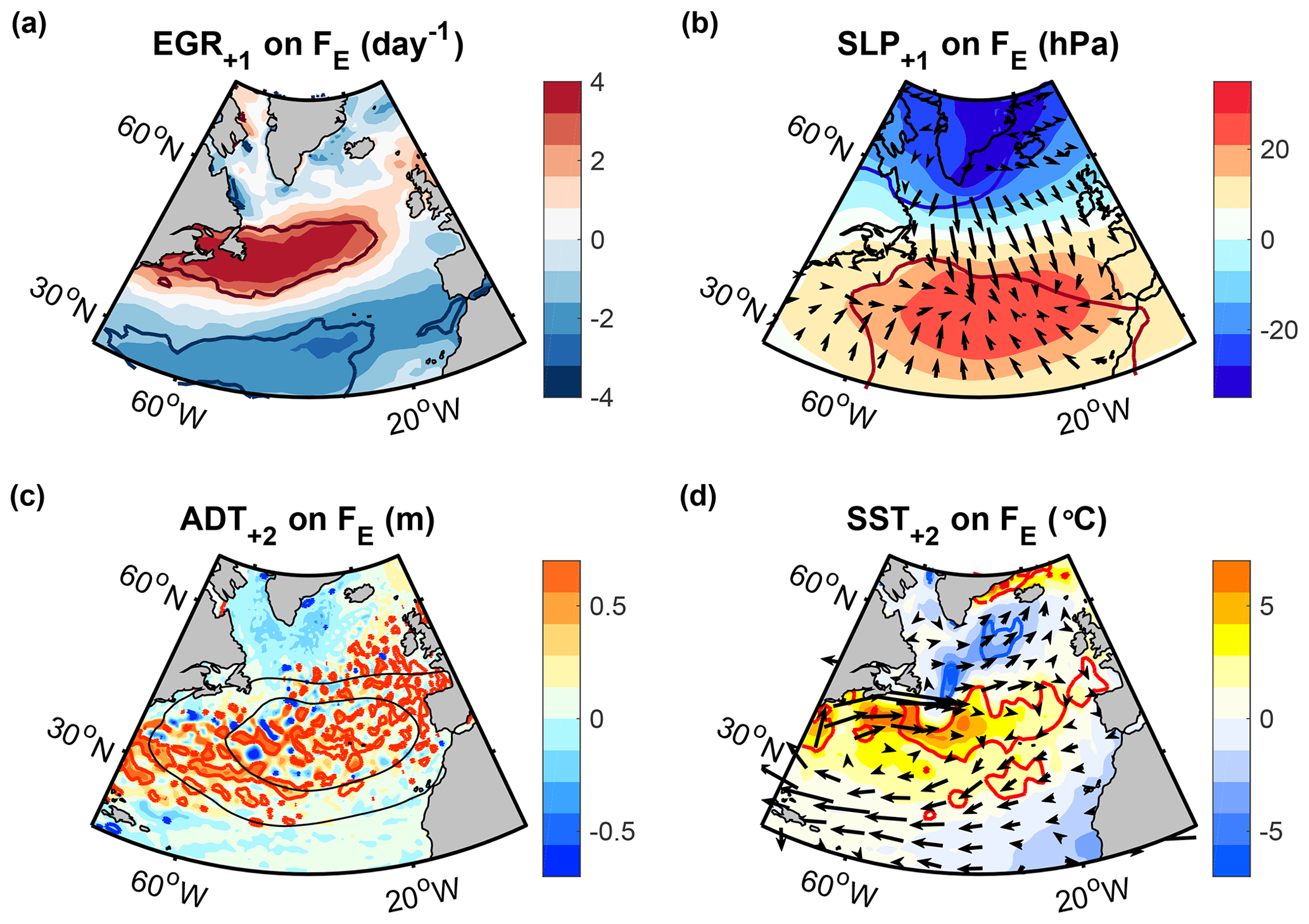
Figure 4Regressions of (a) the maximum Eady growth rate in the lower troposphere, (b) the sea level pressure, (c) the absolute dynamic topography (ADT), and (d) the SST in winter (January through to March) on the freshwater index FE. The anomalies shown in (a) and (b) occur in the first winter after the anomalies, whereas those in (c) and (d) occur in the second winter after the FE summer (indicated by the “+1” and “+2”' in the title). The arrows in (b) show the direction of the associated Ekman transports, while those shown in (d) represent the smoothed geostrophic flow implied by the ADT anomaly. Thin black contours in (c) show the region of Ekman flow convergence from (b). Thick contours in all panels encompass regions that are significant at the 95 % level.
The amplified baroclinic instability manifests itself in a distinct atmospheric circulation anomaly. When an air parcel travels northward across the SST front, it rises because it is warmer than the surrounding air masses. By rising, the air column stretches, acquiring positive vorticity. The opposite occurs when an air parcel travels southward across the front. Consistent with the resulting enhanced baroclinic wave activity, the observations show a cyclonic anomaly north of the SST front and an anticyclonic anomaly to the south (Fig. 4b), representative of a positive NAO phase. Accordingly, we find that after all but the two weakest FE years, the NAO changed from its strongly negative state in summer into a positive state in the subsequent winter. Moreover, over the full period 1979 to 2022, without conditioning on FE years, the correlation between the NAO in summer (July and August) and the NAO in the subsequent winter (January to March) is r≈0.12, which is not significant (p≈0.46). With conditioning on FE years, the correlation is , which is significant (p≈0.03).
The obtained atmospheric circulation anomaly drives a convergent Ekman transport between the subtropical and subpolar gyre (Fig. 4b), leading to an increase in sea level. This Ekman transport is an instantaneous response to the wind forcing (on the investigated timescales), but the resulting increase in sea level and horizontal pressure gradients has longer lasting effects. Thus, we find that the increased sea level and associated ocean instabilities manifest themselves in a broad band of anticyclonic eddies that extends into the second winter after the freshwater anomalies (Fig. 4c). The eddies are not visible in the SST due to the coarser grid spacing of the SST product, compared to the grid spacing of the absolute dynamic topography product. Considering that the mean flow along the eddies is eastward, representing the North Atlantic Current, the integrated effect of the anticyclonic eddies is a reduced eastward speed at the southern edge of the band and an increased eastward speed at the northern edge (Fig. 4d). This circulation pattern has been referred to as inter-gyre gyre circulation (Marshall et al., 2001) and is equivalent to a northward shift in the North Atlantic Current (Kostov et al., 2021; Zhao and Johns, 2014).
The northward shift in the North Atlantic Current implies a warm SST anomaly to the south of the subpolar cold anomaly, not because the water inside the current is anomalously warm but because the current occurs at an anomalously northward location. Thus, the warm SST anomaly to the south of the subpolar cold anomaly is reinforcing the SST gradient, driven by the large-scale winds. It is seen in the first and the second winter after freshwater anomalies (Figs. 1j and 4d). However, in the first winter, the northward shift is partially obscured by the southward expansion of the cold SST anomaly over the eastern North Atlantic, potentially driving enhanced mixing and erosion of the SST front. We point out that the spatial distribution of the surface heat fluxes does not match the SST field (Fig. S1d in the Supplement), indicating that the contribution of the surface heat fluxes to the warm SST anomaly is limited. While this mechanism has been demonstrated using the FE subset, the signals for the FW subset are qualitatively the same but confined to only the first winter.
We summarize that freshwater anomalies are associated with cold anomalies in the subpolar region in winter (Fig. 1j and k). The cold anomalies form part of an enhanced meridional SST gradient, implying a sharper SST front between the subpolar gyre and the subtropical gyre. The sharper SST front is associated with an amplified baroclinic instability in the atmosphere (Fig. 4a) that is characterized by a more cyclonic circulation anomaly over the subpolar gyre and a more anticyclonic anomaly to the south (Fig. 4b). This atmospheric circulation anomaly sets up surface pressure gradients through Ekman transports, which drive a geostrophic flow that contributes to the warm anomaly south of the subpolar cold anomaly (Fig. 4c and d).
The overall effect of the ocean–atmosphere coupling is a sharper SST gradient between the subtropical warm anomaly and the subpolar cold anomaly, which is characteristic of the large-scale SST tripole pattern and associated feedbacks (Czaja and Frankignoul, 2002; Marshall et al., 2001). By being highly correlated with the SST anomalies, the freshwater indices serve as valuable tools for visualizing the associated ocean and atmospheric circulations, reinforcing each other (Figs. 1 and 4). However, we do not causally attribute the SST pattern to freshwater anomalies, and we do not infer that the freshwater anomalies act as a trigger for the characteristic tripole SST pattern.
4.4 Links to European summer weather
The preceding analysis revealed a close statistical link between freshwater anomalies and associated winter conditions. Next, we investigate the SST and atmospheric conditions in subsequent summers. To facilitate the integration of the results into a larger context, we are comparing the regression anomalies obtained from the two subsets with the climatological mean SST and atmospheric conditions in summer, which are similar to the mean conditions across each of the two subsets. We start by investigating the SST field after freshwater anomalies (Fig. 5a–c). In the first summer after stronger freshwater anomalies (again represented by FE), we find that the SST is characterized by an enhanced subpolar cold SST anomaly covering part of the North Atlantic Current in the central North Atlantic (Fig. 5b). In the second summer, the northward shift of the North Atlantic Current is the most pronounced signal, visible as a band of increased SST that extends northeastward across the North Atlantic from Nova Scotia towards the British coast (Fig. 5c).
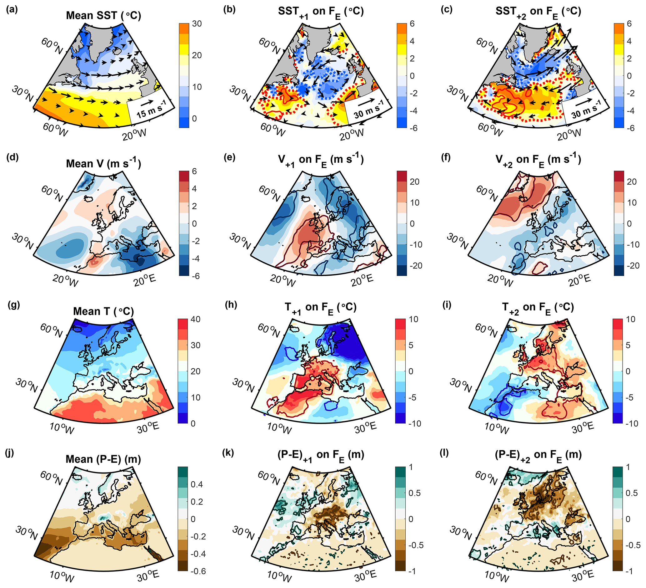
Figure 5Climatological mean (a) SST, (d) meridional winds at 700 hPa, (g) 2 m air temperature, and (j) precipitation minus evaporation in summer (May through to August). Regressions of (b, c) the SST (colour shading) and 700 hPa winds (arrows), (e, f) the meridional winds at 700 hPa, (h, i) the 2 m air temperature, and (k, l) the accumulated precipitation minus evaporation on FE in (b, e, g, k) the first and (c, f, h, l) the second summer (May through to August) after the freshwater anomalies (indicated by the “+1” and “+2” in the titles). We removed large-scale trends from the air temperature to reduce the direct warming effect of greenhouse gases (Sect. 2), and we excluded the anomaly in 2016 since it exhibited a different spatial SST distribution from the other anomalies (Fig. A1). Thick contours encompass regions that are significant at the 95 % confidence level, and the red and blue dotted lines in (b) and (c) delineate the regions in which the SST anomalies exceed 2 ∘C and fall below −2 ∘C.
The SST signal in both summers after the freshwater anomalies implies an increased SST difference between the warm subtropical gyre and the cold subpolar gyre. The exact location of the SST front between the subtropical gyre and the subpolar gyre can differ between the years and is therefore poorly constrained, resulting in reduced significances at individual grid points. However, the increased SST gradient – which is of greater dynamical relevance than absolute SST anomalies – is highly significant. For instance, the SST difference between the region in which the SST anomaly exceeds 2 ∘C and the region in which the SST anomaly falls below −2 ∘C includes a substantial area of the extra-tropical North Atlantic (Fig. 5b and c) and is significantly correlated with the FE index with a correlation coefficient above 0.7 in both summers (r≈0.76 and 0.84 in the first and second summer respectively), with p values well below 0.05.
As in the preceding winters, we find that the atmospheric circulation is aligned with the underlying SST in both the first and second summer after the freshwater anomalies, with the winds at 700 hPa circulating cyclonically around the subpolar cold SST anomalies (Fig. 5b and c). Accordingly, we observe a northward deflection of the lower-tropospheric winds downstream of the cold SST anomaly along the coast (Fig. 5d–f). In the first summer, the northward deflection occurs west off northern Africa, Spain, Portugal, France, and the British coastline (Fig. 5e). In the second summer, the northward deflection of the winds occurs further north to the northwest of the Scandinavian coastline (Fig. 5f), consistent with the more northerly SST front over the North Atlantic (Fig. 5b and c).
The northward deflection of the lower-tropospheric winds forms part of a large-scale atmospheric circulation anomaly, with an increased baroclinic instability across the European coastline, a more cyclonic circulation anomaly over the ocean, and a more anticyclonic circulation anomaly over the continent (not shown but indicated by the arrows in Fig. 5b and c, and the southward wind deflection to the east of the northward deflection in Fig. 5e and f). Thus, the large-scale atmospheric circulation is similar to the conditions described in winter (Fig. 4b). In both seasons, there is a cyclonic atmospheric circulation anomaly above the cold SST anomaly. In summer, however, the anticyclonic circulation occurs over the continent instead of over the subtropical North Atlantic. We hypothesize that the difference is due to the faster surface heating of the land in spring and summer, which increases the surface temperature difference between the colder subpolar ocean surface and the warmer continent and which hence favours an increased atmospheric instability across the coastline.
In line with the shifted large-scale atmospheric circulation anomalies, we observe relatively warmer and drier air over northern Africa and southwest Europe in the first summer after stronger freshwater anomalies and relatively warmer and drier air over northwest Europe in the second summer (Fig. 5g–l). In the first summer, the maximum warm anomalies extend from Morocco and Algeria northward to France and southern Germany, while the maximum dry anomalies occur further to the east covering large parts of southwest Europe, including Italy and Greece. In the second summer after the freshwater anomalies, the maximum warm anomalies occur over central to northern Europe, including Germany, France, the UK, Poland, and southern Sweden, while the maximum dry anomalies again extend further eastward, including Finland and the Baltic countries. Considering that precipitation anomalies preferentially occur along trailing cold fronts and are shifted southward relative to cyclone centres (Booth et al., 2018; Kodama et al., 2019), the observed displacement of the dry anomalies relative to the warm anomalies is expected from their locations within individual weather systems and consistent with other studies (Yu et al., 2023).
Placing the identified atmospheric anomalies into a larger context described in the literature, we find that it is representative of blocking anticyclones (Brunner et al., 2018; Kautz et al., 2022). In summer, blocking anticyclones over Europe are typically associated with increased surface pressure and higher surface air temperatures (Brunner et al., 2018; Kautz et al., 2022). Considering that the maximum temperature anomalies in summers after enhanced FE freshwater anomalies occur east of the northward wind deflection, in the centre of the anticyclonic circulation anomaly, the location of the increased air temperature anomalies is consistent with earlier studies which have attributed the warm anomalies to enhanced shortwave radiation (Kautz et al., 2022; Pfahl, 2014; Sousa et al., 2018). Moreover, the occurrence of the dry anomalies to the east of the warm surface air temperature anomalies likely results from a reduced passage of cyclonic weather systems, which are blocked by the large-scale anticyclonic circulation anomalies (Sousa et al., 2017).
A downside of the statistical approach arises from the sensitivity of European summer weather to the exact location of the SST front between the subtropical and subpolar gyres. Small deviations in the spatial characteristics of the SST pattern and lower-tropospheric circulation between 2 years can lead to shifts in the location of the maximum warm and dry anomalies over Europe, partially cancelling each other out. Thus, we found that the spatial patterns in summer 2016 did not match those of the other years included in the FE subset (Fig. A1). The cold SST anomaly extended further south of the North Atlantic Current, resulting in enhanced mixing and a patchy meridional SST gradient just west of the European coast with two cold anomalies of reduced amplitudes. Consistent with the underlying SST field, we identified a split zonal wind between ∼0 and ∼10∘ E, with one branch extending northward along the European coastline and another one crossing the southern Mediterranean Sea. Accordingly, one warm surface air temperature anomaly covered northern Africa and another warm anomaly occurred along the northwest European coastline (Fig. A1). So, even though the spatial SST pattern in summer 2016 did not match those in the other summers, we still identify the same close relationship between the SST, the tropospheric winds, and European weather anomalies.
Similar to the FE freshwater anomalies, freshwater anomalies associated with the FW subset are also followed by a cold SST anomaly in the subsequent summer. However, compared to FE freshwater anomalies, the cold SST anomalies associated with the FW index are smaller and confined to the central and western North Atlantic off the coast of Newfoundland, with the regressions peaking in July and August (Fig. 6a). Consequently, we observe a sharp northward deflection of the winds just eastward of the cold anomaly and further west compared to the FE subset (Fig. 6b). Likewise, the warm air temperature anomalies over Europe also occur further west and are centred over France, Great Britain, Belgium, and northern Spain, extending westward off the coast, while the dry anomalies extend eastward to the Baltic Sea region and northern Poland (Fig. 6c and d).
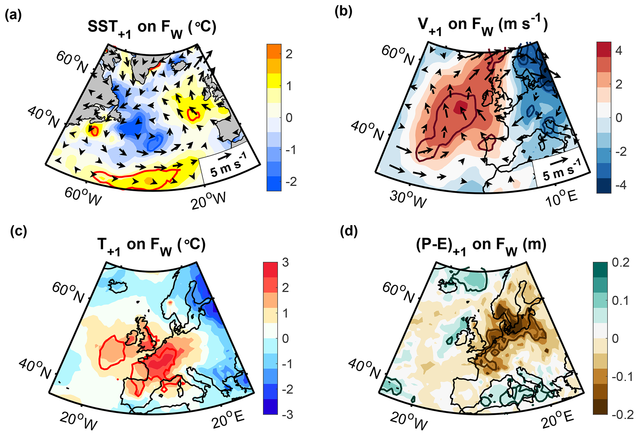
Figure 6Regressions of (a) SST (colour shading) and 700 hPa winds (arrows), (b) meridional winds at 700 hPa, (c) 2 m air temperature, and (d) precipitation minus evaporation in summer (July and August) on FW from the preceding summer, again after subtracting large-scale trends from the air temperature. Thick contours encompass regions that are significant at the 95 % confidence level.
Overall, we find that the regressions of the SST and atmospheric circulation on FW are weaker compared to those on FE, consistent with weaker freshwater anomalies (Fig. 2) and smaller regression slopes (Fig. 1l), implying weaker sensitivities to the freshwater index and associated atmospheric circulation in the preceding summer. Yet, despite differences in the location and magnitude of the anomalies, the overall patterns are qualitatively similar after FE and FW freshwater anomalies: both types of freshwater anomalies are characterized by a cold SST anomaly and northward deflection of the lower-tropospheric winds over the North Atlantic in the subsequent summer. In both cases, the obtained, large-scale atmospheric circulation anomaly is associated with warmer and drier weather over parts of Europe. Moreover, considering that – from all the years included in each subset (17 and 8 respectively) – only summer 2016 exhibited a spatially diverging SST pattern, the results suggest that (1) the statistical method is overall successful in selecting years with similar spatial structures and (2) the spatial coherency for which we selected in winter is, in most cases, maintained through to the subsequent summer.
4.5 Significance and robustness
The significance of the relationships between the freshwater indices and the ocean and atmospheric conditions in the subsequent winter and summer was assessed by Student t tests. Importantly, the subsampling was based on the SST and freshwater anomalies only. Thus, it does not affect the relationship between the subsampled index and any variable that is statistically independent of freshwater (or the SST). If a random variable has no actual connection to freshwater anomalies, the probability for randomly obtaining a significant statistical link by chance remains the same.
Based on the Student t tests, we obtained statistically significant links above the 95 % confidence level, indicating that the probability for randomly obtaining the identified connections between North Atlantic freshwater anomalies in winter and the subsequent European summer weather is less than 5 %. To ensure that the results are robust, we repeated the regressions by changing the number of years included in the subsampling and by excluding anomalies in consecutive years (Sect. S2). In all cases, we find that the identified links are robust, which is consistent with the scatter diagram (Fig. 1l), showing that there are no outliers or clusters of values responsible for the high correlations.
A downside of the FE and FW indices arises from the limited set of years, raising the question of if the relationship between the SST, SSS, and subsequent atmospheric anomalies holds generally or only over the selected subsets. To address this question, we use an un-subsampled SST-based index covering all years. As before, we avoid potential influences of a spatially uniform warming trend by using the spatial SST differences between the subpolar and the subtropical gyre (“ΔSST”) rather than absolute cold anomalies. Specifically, we use the observed SST difference between regions enclosed by the 95 % lines in Fig. 1j in any given year. We selected these regions since they cover such a large area of the subpolar and northern subtropical region and clearly define both regions. However, the results are not sensitive to this choice. The resulting time series is shown in Fig. 7a.
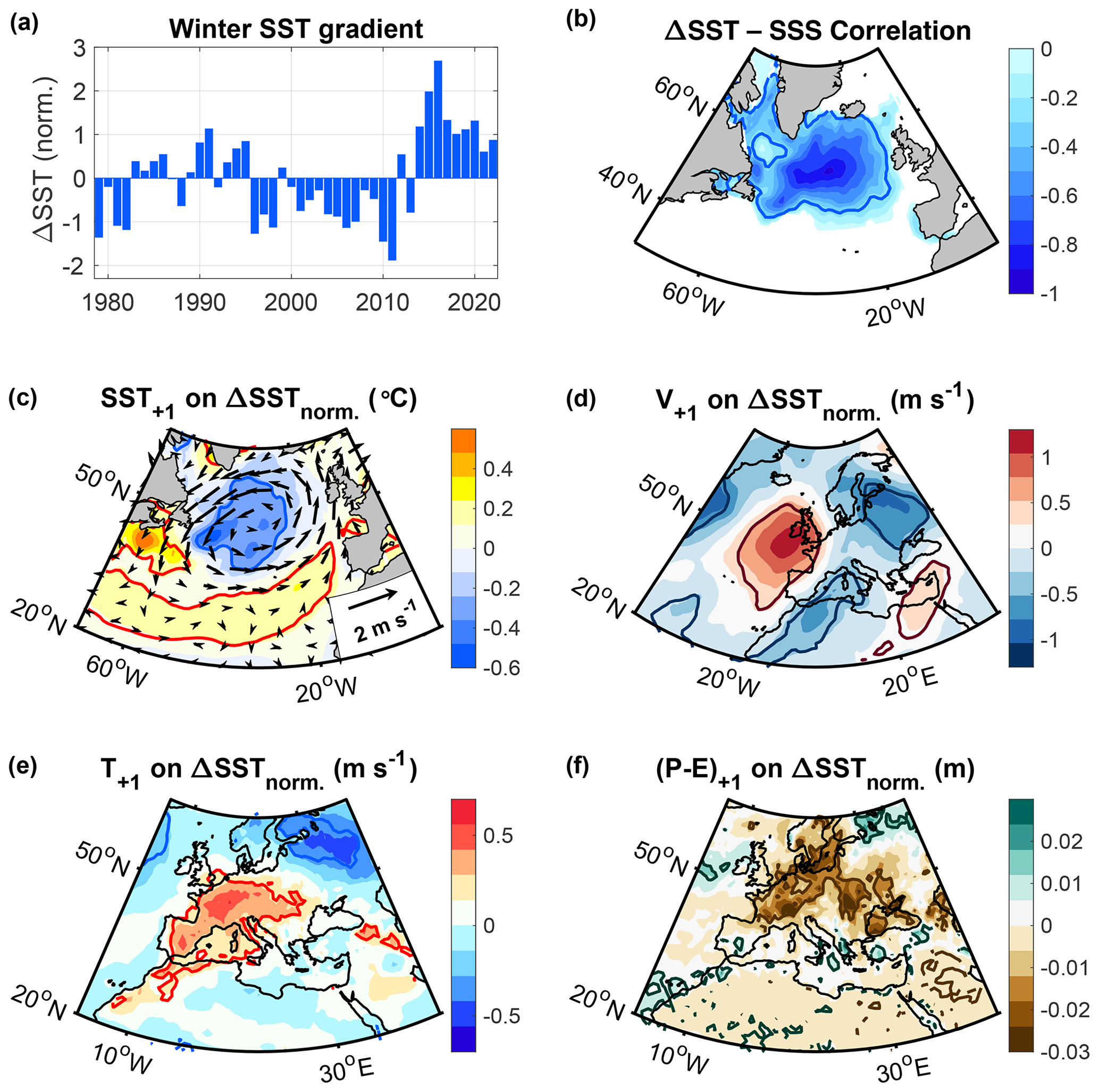
Figure 7(a) ΔSST index corresponding to the SST difference between the subtropical warm anomaly and the subpolar cold anomaly, enclosed within the 95 % confidence lines in Fig. 1j. The time series of the SST difference has been normalized by its standard deviation. (b) Correlation between the ΔSST index, shown in (a), and the sea surface salinity anomaly in the same winter (January through March), estimated from the surface mass balance (Sect. S1). (c–f) Regressions of (c) SST (colour shading) and 700 hPa winds (arrows), (d) meridional winds at 700 hPa, (e) 2 m air temperature, and (f) precipitation minus evaporation in summer (July and August) onto the ΔSST index from the preceding winter (a), again after subtracting the large-scale trends from the air temperature. Thick contours encompass regions that are significant at the 95 % confidence level.
Evaluating the surface mass balance associated with the new ΔSST index, we again find that none of the terms on the righthand side of Eq. (5) can account for the mass increase, implied by the associated cold, subpolar SST anomaly (Sect. S1). Thus, we conclude that the cold anomaly can only be explained by the simultaneous existence of a freshwater anomaly, allowing us to infer the variability and spatial distribution of surface freshwater with an overall uncertainty of ∼6 % which results from assuming density compensation. The correlation of the estimated freshwater variability with the ΔSST index extends over the full subpolar region, with maximum amplitudes of up to ∼0.8 occurring in the eastern subpolar gyre (Fig. 7b). This correlation is slightly smaller than those obtained for the other two freshwater indices, but the index now covers all 44 years.
Considering the significant link between the ΔSST index and surface freshwater in the subpolar region, we use it as a new freshwater index and examine the ocean and atmospheric conditions in the subsequent summer. Inspection of the SST shows that a stronger ΔSST index in winter is associated with a pronounced cold SST anomaly over the central subpolar region in the subsequent summer (Fig. 7c). The atmospheric circulation is aligned with the underlying SST field, with the winds at 700 hPa circulating cyclonically around the cold, subpolar SST anomaly (Fig. 7c). To the east of the cold SST anomaly, the winds are deflected northward along the European coastline (Fig. 7d). Again the northward-deflected winds form part of a large-scale atmospheric circulation anomaly that is associated with warmer and drier weather over Europe. The associated warm anomalies extend over Spain; Italy; France; the Netherlands; and parts of Germany eastward to Austria, Hungary, and Slovakia, while the dry anomalies occur further northeastward, covering France; the Netherlands; Denmark; and parts of northern Germany, Poland, and Ukraine (Fig. 7e and f).
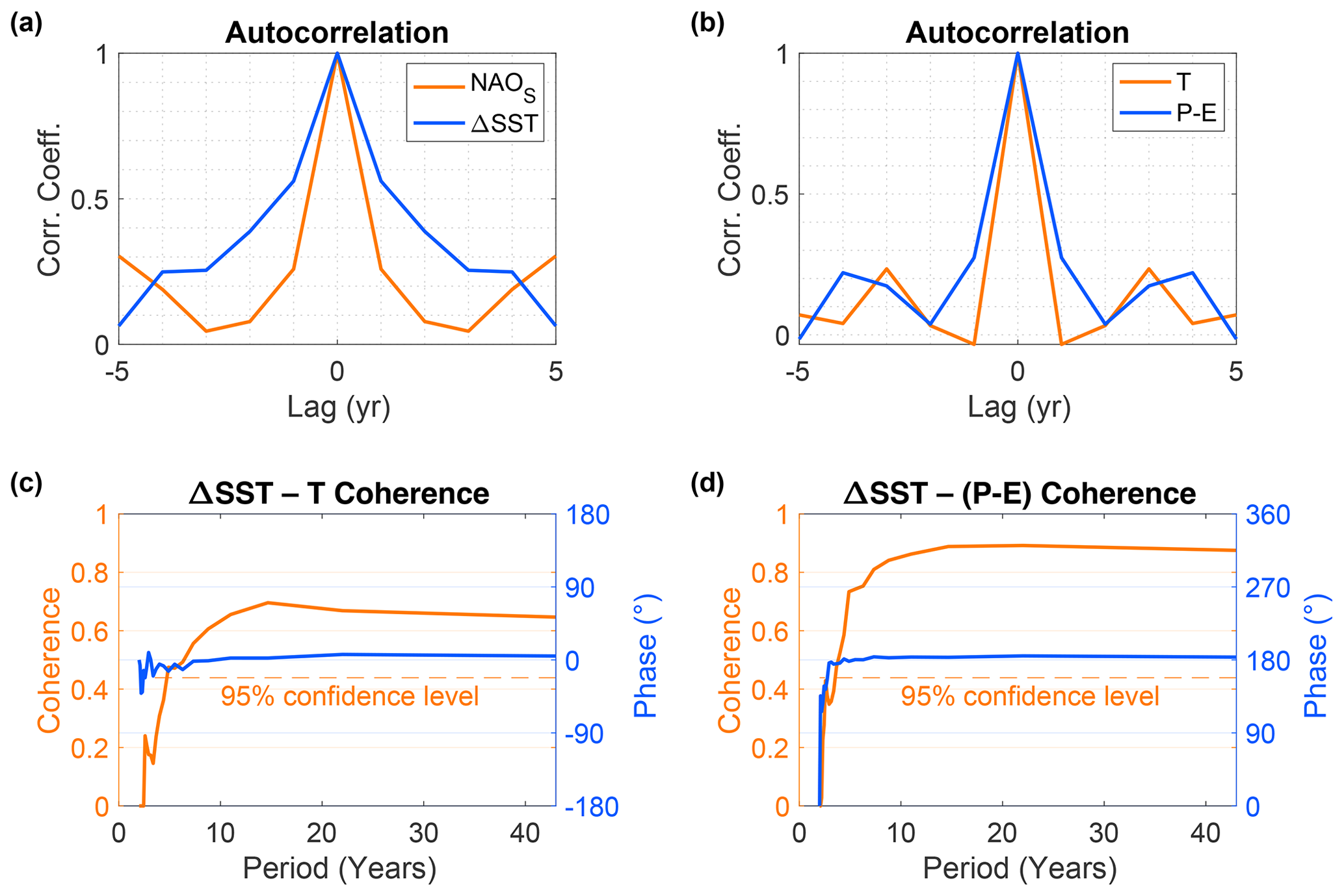
Figure 8(a, b) Autocorrelations of (a) the NAO index in summer (July and August) and the ΔSST index in winter (Fig. 7a) and (b) the 2 m air temperature and precipitation minus evaporation anomalies in summer (July and August), averaged over the regions enclosed by the 95 % confidence lines in Fig. 7e and f. (c, d) Multi-taper coherence and phase shift estimates for the ΔSST index in winter (January to March) and (c) the 2 m air temperature and (d) precipitation minus evaporation in the subsequent summer (July and August), again within the regions enclosed by the 95 % confidence lines in Fig. 7e and f. We used eight tapers. The 95 % confidence estimates are based on Amos and Koopmans (1963) after correcting for the bias inherent in coherence estimates (Priestley, 1982).
Unlike the summer NAO, the new, SST-based index has higher autocorrelations (Fig. 8a), which we attribute to enhanced low-frequency variability in the North Atlantic climate in winter. We still assume that interannual variability substantially contributes to the correlations due to the high, interannual variability in European summer weather, reflected in low autocorrelations (Fig. 8b). Nonetheless, to assess the contribution of low-frequency variability to the obtained links, we lowpass filter European summer weather with a Hanning filter, using a window size of three summers to approximate the higher autocorrelations of the ΔSST index (Sect. S2). After accounting for the reduced number of independent samples in the significance tests with , where N here refers to the number of data points, Δt is the time interval between them, and Te is the e-folding timescale of the autocorrelations (Leith, 1973), we still obtain statistically significant relationships, but the amplitudes of the regressions are reduced (Fig. S13), indicating that high-frequency, interannual variability substantially contributed to the relationship obtained from the unfiltered time series (Fig. 7).
To further assess the timescales on which the identified relationship holds and is significant, we carry out a multi-taper coherence analysis. Specifically, we calculate the coherence between the ΔSST index and the temperature and precipitation minus evaporation anomalies in the regions in which we identified a significant link from the regressions (Fig. 7e and f). Inspection of the coherence estimate shows that both temperature and precipitation minus evaporation over Europe are significantly linked to freshwater variations in the subpolar region on timescales from a few years to decades (Fig. 8c and d). The coherence between the ΔSST index and the precipitation minus evaporation anomaly is particularly high and well above the 95 % significance line (Fig. 8d). The associated phase shifts are relatively constant at 0∘ for the air temperature (indicating a positive correlation) and 180∘ for precipitation minus evaporation (implying anti-correlation). We used eight tapers, which is a standard value. However, the results are not sensitive to this choice.
We conclude that the link between cold, fresh ocean anomalies in the subpolar North Atlantic region in winter and warm, dry atmospheric anomalies over Europe in the subsequent summer is robust, significant at both higher and lower frequencies, and independent of the spatial and temporal characteristics of the freshwater index that is used.
4.6 Predictability of European summer weather
The preceding analyses revealed significant links between North Atlantic freshwater anomalies and European summer weather in subsequent years. This raises the question of the extent to which this link can be used to predict European summer weather in advance. Thus, we next assess the predictability based on the explained variance in the observations, estimated by means of the squared correlation coefficient with the freshwater indices.
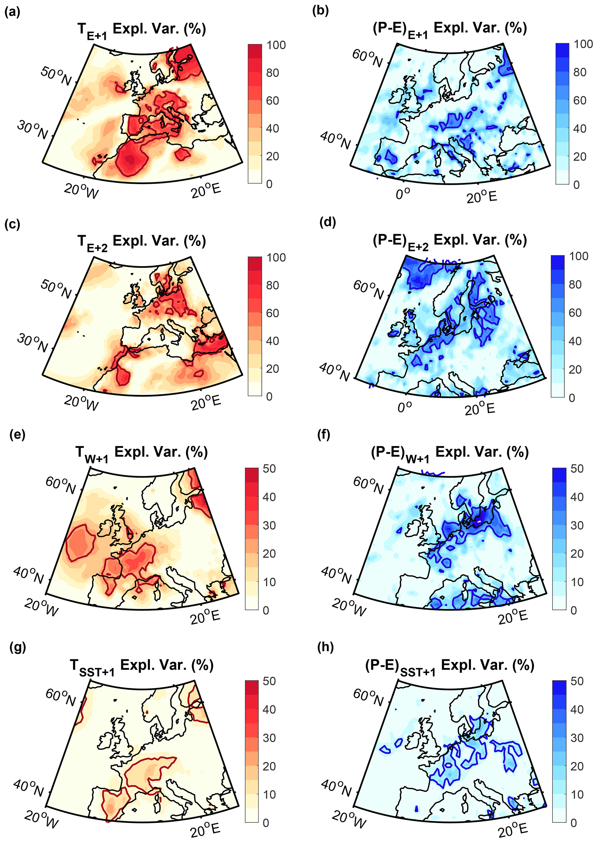
Figure 9Variances explained by (a–d) FE, (e, f) FW, and (g, h) the ΔSST index of (a, c, e, g) the 2 m air temperature and (b, d, f, h) precipitation minus evaporation after freshwater anomalies. “+1” and “+2” in the titles refer to the first and second summer after the freshwater anomaly. We again excluded the 2016 freshwater anomaly from FE since its spatial SST anomaly was inconsistent with the others (Fig. A1). Thick contours delineate the regions in which the correlation is significant at the 95 % confidence level, assessed by means of two-sided Student t tests. The explained variances were obtained from the squared correlation coefficients. Please note the different colour scales.
The variance in the near-surface temperature and precipitation minus evaporation anomalies, explained by the FE subset, reaches and even exceeds 80 % over large parts of Europe (Fig. 9a–d). For the FW subset, the explained variance drops to ∼50 % (Fig. 9e and f), and for the ΔSST index, the explained variance drops further to ∼20 % (Fig. 9g and h), as expected from the trade-off between the number of years included in the index and the associated correlations with freshwater anomalies in the subpolar North Atlantic region in winter and European weather anomalies in the subsequent summer.
Overall, we find that the higher the correlation is between the initial freshwater anomaly and its index, the higher the variance of European summer weather also is that the index subsequently explains. The FE index, in particular, has an extremely high correlation with the initial freshwater anomaly of over ∼0.9 (Fig. 2c) and explains over 80 % of the variance of European summer weather. Considering that all indices represent fresh and cold SST anomalies in the subpolar region and notwithstanding the small sample sizes or the reduced correlations, these results indicate that accurate estimates of the sea surface salinity in the subpolar region can serve as valuable constraints for the subsequent European summer weather. Specifically, the amount of the variance in European summer weather, explained by the freshwater anomaly, depends on the location, amplitude, and type of the freshwater anomaly in the subpolar region in the preceding winter.
4.7 Warm summers in Europe
The preceding analyses showed that two types of freshwater anomalies with opposite atmospheric drivers (characterized by a high and a low NAO states in the preceding summer) are associated with cold SST anomalies over the North Atlantic in winter. The resulting increased SST fronts are maintained through to the subsequent summer, when (aligned with the underlying SST fronts) the lower-tropospheric winds are deflected northward east of the cold anomaly and along the European coastline. The winds form part of large-scale atmospheric circulation anomalies that lead to warmer, drier weather over Europe, with the location of the warm and dry anomalies being sensitive to the exact location, strength, and type of freshwater anomaly in the preceding winter. In this last section, we investigate if the warmest European summers can in turn be linked back to a freshwater anomaly in the preceding year. Thus, we assess the extent to which enhanced freshwater anomalies are not only a sufficient but also a necessary condition for warmer European summers.
Based on composites, we find that the 10 warmest relative to the 10 coldest summers in western Europe were associated with a dry anomaly to the east of the warm air temperature anomaly; a northward deflection of the wind at 700 hPa west of Portugal, France, and Britain; and a pronounced cold SST anomaly in the subpolar North Atlantic (Fig. 10a–e). Using a surface mass balance (Sect. S1), we again identify a significant freshwater anomaly in the preceding winter, with the freshwater anomaly covering a large part of the subpolar North Atlantic (Fig. 10f). Selecting different regions for the temperature variability over Europe (Fig. 10a and b) shifts the location of the atmospheric circulation pattern and the location of the maximum North Atlantic SST gradient and freshwater anomalies but does not qualitatively alter the results.
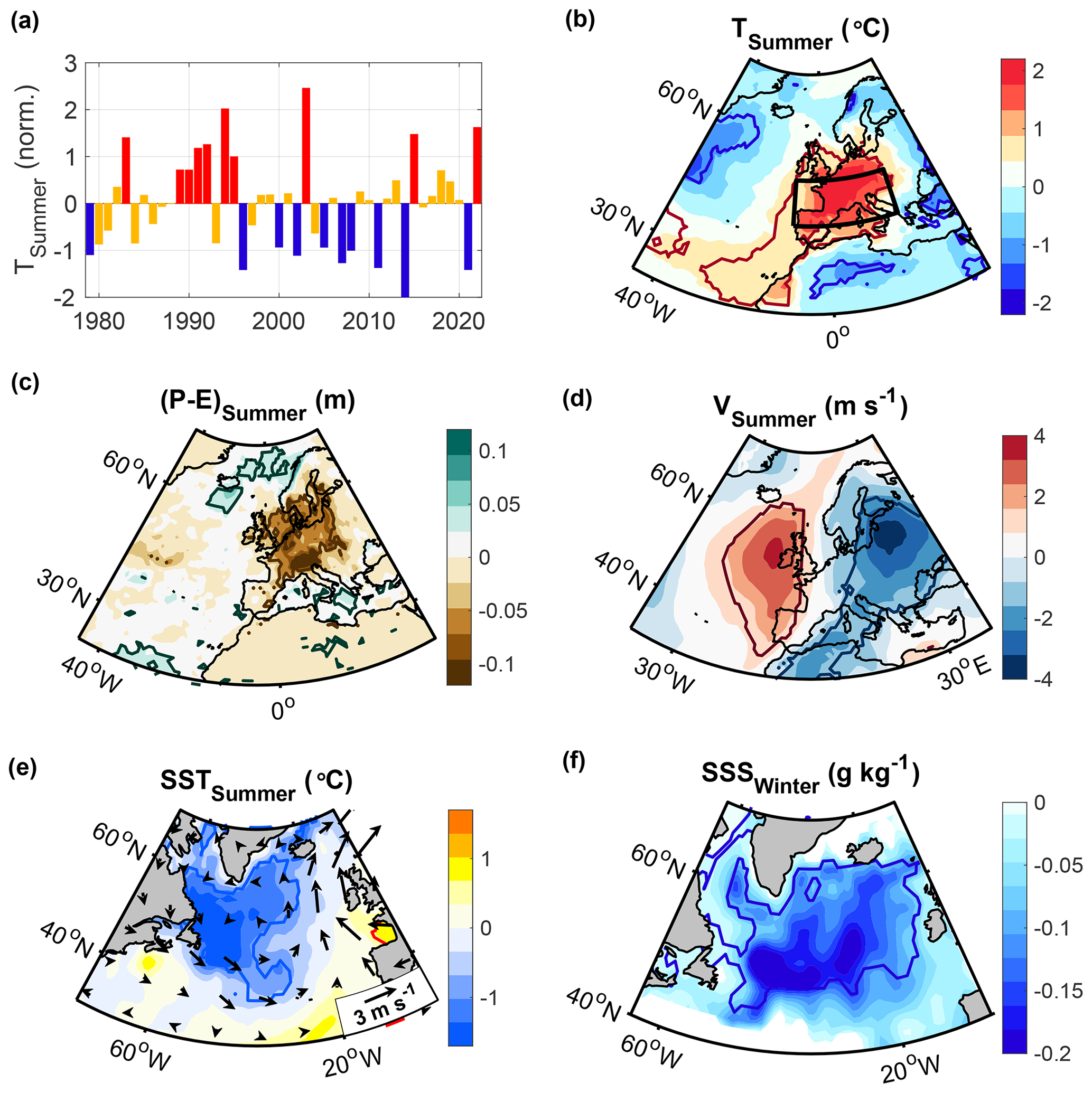
Figure 10(a) Variability in the de-trended 2 m air temperature anomaly over land within the box shown in (b) during summer (July and August). (b–e) Composites of (b) the 2 m air temperature, (c) precipitation minus evaporation, (d) the meridional winds at 700 hPa, and (e) the SST (colour shading) and the 700 hPa winds (arrows) for the 10 warmest minus the 10 coldest summers, shown in (a). (f) Same as in (b)–(e) but for the sea surface salinity anomaly in the preceding winter, obtained from a surface mass balance (Sect. S1). Contours delineate the regions that are significant at the 95 % confidence level, assessed by means of two-sided, two-sample t tests.
The similarity of the ocean and atmospheric conditions with those described in the preceding sections supports the relevance of freshwater anomalies in winter for the subsequent ocean–atmosphere evolution into the summer. In addition, the composites suggest that enhanced freshwater anomalies in the subpolar North Atlantic in winter can serve as early warning signs of Europe's warmest and coldest summers approximately half a year in advance.
In this study, we examined the link between North Atlantic freshwater anomalies and European weather in subsequent summers. Given the limitations of currently available salinity observations, we estimated the variability in freshwater based on a surface mass balance analysis. We further investigated the statistical links between the obtained freshwater anomalies in winter and the subsequent European summer weather by applying regression and correlation analyses, composite analyses, and multi-tapered coherence analyses.
Combined, the analyses reveal a significant relationship between freshwater anomalies in winter and European weather in subsequent summers. Specifically, we found that enhanced freshwater anomalies are associated with colder, subpolar SST anomalies and an increased SST difference between the warm subtropical and the cold subpolar gyre in winter. The increased, meridional SST gradient is linked to an amplified atmospheric instability and a large-scale atmospheric circulation anomaly with a more cyclonic circulation over the subpolar region and an anticyclonic anomaly to the south. This atmospheric circulation anomaly induces a northward shift in the North Atlantic Current which contributes to a warm anomaly to the south of the subpolar cold anomaly, amplifying the meridional SST gradient. In subsequent summers, the lower-tropospheric winds are deflected northward over the North Atlantic in the wake of the cold SST anomaly, aligned with the underlying SST fronts. This northward deflection of the winds forms part of a large-scale atmospheric circulation anomaly consisting of a more cyclonic circulation over the subpolar North Atlantic region and a more anticyclonic circulation over parts of Europe, giving rise to warmer and drier weather over Europe.
The atmospheric circulation in summer is characteristic of blocking anticyclones over Europe described in earlier studies (Brunner et al., 2018; Kautz et al., 2022). Thus, the warm surface anomalies can be explained by increased shortwave radiation in the centre of the anticyclones (Kautz et al., 2022; Pfahl, 2014; Sousa et al., 2018), while the dry anomalies to the east can be explained by the blocking of cyclonic weather systems (Sousa et al., 2017). Further studies are required to quantify the relative contributions of ocean and atmospheric drivers to the large-scale atmospheric circulation anomaly in summer, their uncertainties, and the role of freshwater as a potential trigger of the identified chain of events. However, the obtained evolution of freshwater anomalies follows the chain of events expected from theory. In addition, the statistical links identified in this study suggest that the estimation of the extent, amplitude, and type of freshwater anomaly in any given winter can constrain the subsequent European summer weather, based on the evolution of past freshwater anomalies and the associated explained variances.
Current numerical weather prediction systems show very limited to no forecast skill for European summer weather (Arribas et al., 2011; Dunstone et al., 2018). Thus, the existence of a link between North Atlantic freshwater anomalies and European summer weather indicates new potential to enhance the predictability of European summer weather a year in advance. Further studies that improve the representation of North Atlantic freshwater variations in models and that quantify the predictability arising from them are therefore desirable. In addition, targeted observational networks that monitor the variability in freshwater anomalies may help improve current forecast systems.
Linking European summer weather with North Atlantic freshwater anomalies, as opposed to linking it to SST anomalies only, has the advantage that the occurrence of freshwater anomalies is easier to predict into the future than SST anomalies due to having more narrowly defined drivers. In this study, we attributed the freshwater anomalies to only two main drivers on interannual timescales. One type of freshwater anomaly was linked to a change in the subpolar gyre circulation. The other type of freshwater anomaly was linked to enhanced runoff and melting. Runoff and melting, specifically, largely occur in summer, giving rise to a longer predictive timescale: half a year in advance of the cold and fresh anomalies in winter and 1 year in advance of the subsequent European summer weather anomalies.
The melting of land and sea ice are expected to increase (Notz and Stroeve, 2018; Briner et al., 2020) over the coming decades, resulting in an enhanced freshwater discharge into the North Atlantic. With stronger freshwater anomalies, our results indicate an increase in the risk of warm, dry European summers and of heat waves and droughts accordingly. Unfortunately, global climate models have difficulties in capturing the hydrographic structure and freshwater distribution in the subpolar North Atlantic (Menary et al., 2015; Heuzé, 2017; Liu et al., 2017; Sgubin et al., 2017; Mecking et al., 2017; Wu et al., 2018). Considering the identified links between freshwater anomalies and subsequent ocean–atmosphere evolution, our results suggest that models may miss a key source of climate variability and potential long-range predictability.
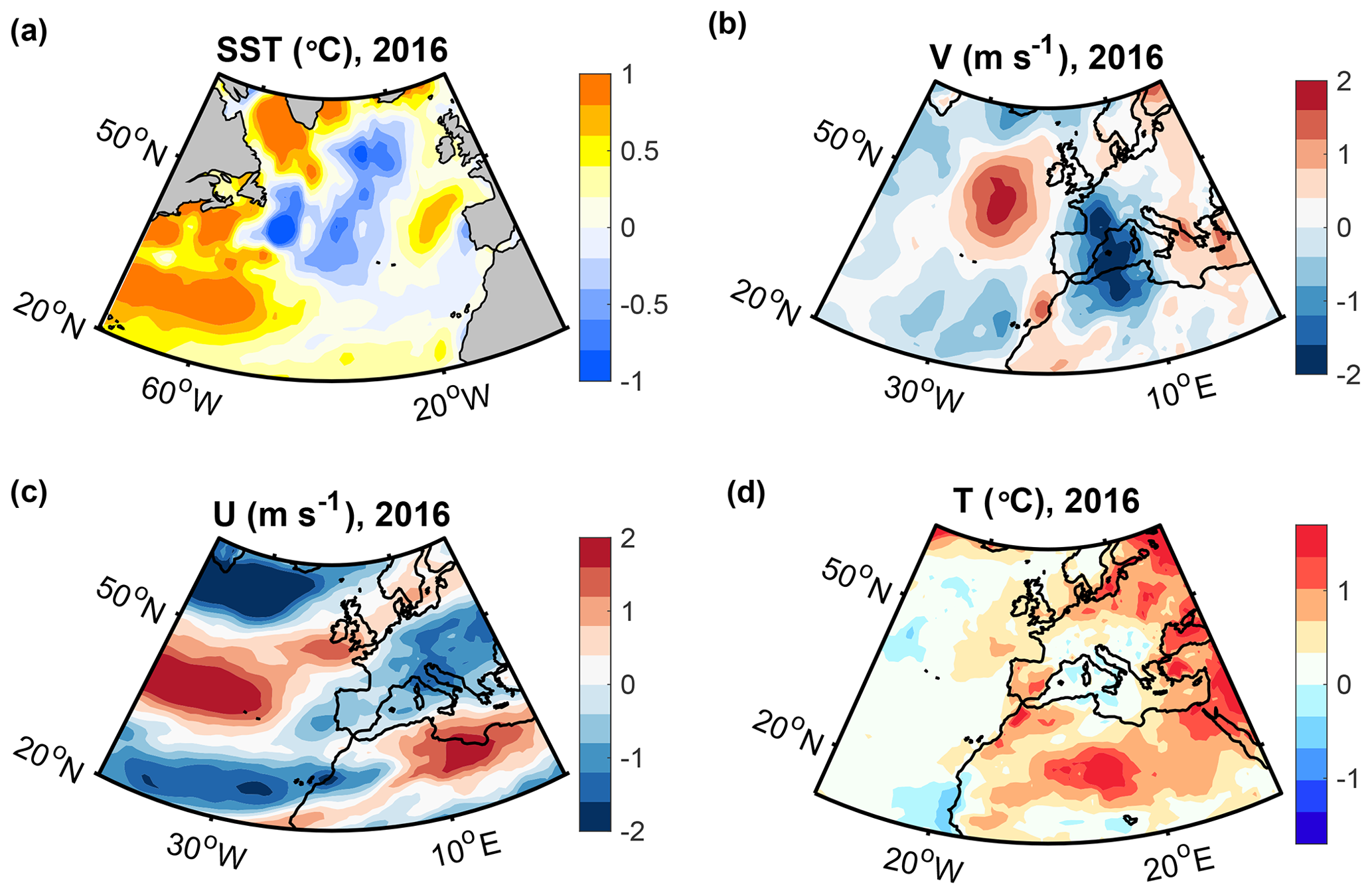
Figure A1Anomalies of (a) SST, (b) the meridional winds and (c) the zonal winds at 700 hPa, and (d) the 2 m air temperature in summer (May through to August) in 2016, relative to the climatological mean.
Table A1List of years included in the three freshwater indices FE, FW, and ΔSST. The years listed for FE and FW correspond to the years of the summer NAO index in July and August, while the period listed for ΔSST corresponds to the years of the SST anomalies in winter (January to March).
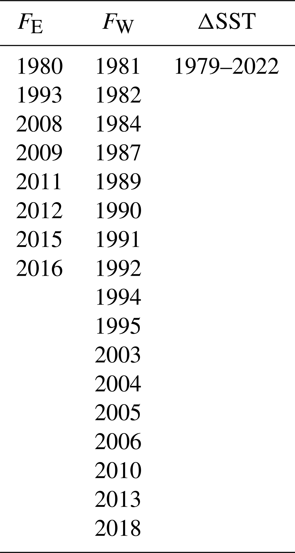
This study is only based on publicly available data and standard analysis techniques. The NAO data are based on rotated principal component analysis (Barnston and Livezey, 1987; Chen and van den Dool, 2003; van den Dool et al., 2000) and available from NOAA: https://www.cpc.ncep.noaa.gov/products/precip/CWlink/pna/nao.shtml (last access: 9 March 2023). We further used the merged SST dataset (Shea et al., 2022), which is available at https://doi.org/10.5065/r33v-sv91. The merged dataset includes SST data from NOAA (Reynolds et al., 2002) and the Hadley Centre (Rayner et al., 2003). Absolute dynamic topography data are distributed by the Copernicus Marine Environment Monitoring Service (2023, https://doi.org/10.48670/moi-00148). ERA5 data (Hersbach et al., 2023) can be obtained from the Copernicus Climate Change Service (C3S) at https://doi.org/10.24381/cds.adbb2d47. The mixed layer Argo database (Holte et al., 2017) is available at http://mixedlayer.ucsd.edu (last access: 11 January 2018). MATLAB codes can be obtained from the corresponding author. This study employed the GSW Oceanographic Toolbox (McDougall and Barker, 2011), which is available at http://www.teos-10.org/software.htm (last access: 23 May 2020).
The supplement related to this article is available online at: https://doi.org/10.5194/wcd-5-109-2024-supplement.
MO conceived the study, carried out the analyses, and was lead writer of the text. NPH and JS provided guidance in the framing of the study; SB helped to revise the paper. All authors contributed to the development of the manuscript in multiple discussions.
The contact author has declared that none of the authors has any competing interests.
Publisher's note: Copernicus Publications remains neutral with regard to jurisdictional claims made in the text, published maps, institutional affiliations, or any other geographical representation in this paper. While Copernicus Publications makes every effort to include appropriate place names, the final responsibility lies with the authors.
We thank NOAA/OAR/ESRL and the Hadley Centre for providing the SST data, the Copernicus Marine Service for distributing the altimetry products, the European Centre for Medium-Range Weather Forecasts for developing the reanalysis ERA5 product, and the NOAA Physical Sciences Laboratory for facilitating access to the climate model outputs. We also thank Xavier Fettweis for providing output from the Greenland climate model MAR. This study was funded through the grants ACSIS (NE/N018044/1), CLASS (NE/R015953/1) and CANARI (NE/W004984/1) from the UK National Environmental Research Council.
This research has been supported by the Natural Environment Research Council (grants CLASS: NE/R015953/1; CANARI: NE/W004984/1; and DIMSUM: NE/Y005090/1).
This paper was edited by Stephan Pfahl and reviewed by two anonymous referees.
Amos, D. E. and Koopmans, L. H.: Tables of the distribution of the coefficient of coherence for stationary bivariate Gaussian processes, vol. 483, Sandia Corporation, https://doi.org/10.2172/4727236, 1963. a
Arribas, A., Glover, M., Maidens, A., Peterson, K., Gordon, M., MacLachlan, C., Graham, R., Fereday, D., Camp, J., Scaife, A., Xavier, P., McLean, P., Colman, A., and Cusack, S.: The GloSea4 ensemble prediction system for seasonal forecasting, Mon. Weather Rev., 139, 1891–1910, 2011. a
Bamber, J., van den Broeke, M., Ettema, J., Lenaerts, J., and Rignot, E.: Recent large increases in freshwater fluxes from Greenland into the North Atlantic, Geophys. Res. Lett., 39, L19501, https://doi.org/10.1029/2012GL052552, 2012. a
Bamber, J., Tedstone, A., King, M., Howat, I., Enderlin, E., van den Broeke, M., and Noel, B.: Land ice freshwater budget of the Arctic and North Atlantic Oceans: 1. Data, methods, and results, J. Geophys. Res.-Oceans, 123, 1827–1837, 2018. a, b, c, d
Bao, S., Wang, H., Zhang, R., Yan, H., and Chen, J.: Comparison of satellite-derived sea surface salinity products from SMOS, Aquarius, and SMAP, J. Geophys. Res.-Oceans, 124, 1932–1944, 2019. a, b
Barnes, E. A.: Revisiting the evidence linking Arctic amplification to extreme weather in midlatitudes, Geophys. Res. Lett., 40, 4734–4739, 2013. a
Barnston, A. G. and Livezey, R. E.: Classification, seasonality and persistence of low-frequency atmospheric circulation patterns, Mon. Weather Rev., 115, 1083–1126, 1987. a, b
Blackport, R. and Screen, J. A.: Insignificant effect of Arctic amplification on the amplitude of midlatitude atmospheric waves, Sci. Adv., 6, eaay2880, https://doi.org/10.1126/sciadv.aay2880, 2020. a
Böning, C. W., Behrens, E., Biastoch, A., Getzlaff, K., and Bamber, J. L.: Emerging impact of Greenland meltwater on deepwater formation in the North Atlantic Ocean, Nat. Geosci., 9, 523–527, 2016. a
Booth, J. F., Naud, C. M., and Willison, J.: Evaluation of extratropical cyclone precipitation in the North Atlantic basin: An analysis of ERA-Interim, WRF, and two CMIP5 models, J. Climate, 31, 2345–2360, 2018. a
Briner, J. P., Cuzzone, J. K., Badgeley, J. A., Young, N. E., Steig, E. J., Morlighem, M., Schlegel, N.-J., Hakim, G. J., Schaefer, J. M., Johnson, J. V., Lesnek, A. J., Thomas, E. K., Allan, E., Bennike, O., Cluett, A. A., Csatho, B., de Vernal, A., Downs, J., Larour, E., and Nowicki, S.: Rate of mass loss from the Greenland Ice Sheet will exceed Holocene values this century, Nature, 586, 70–74, 2020. a
Brunner, L., Schaller, N., Anstey, J., Sillmann, J., and Steiner, A. K.: Dependence of present and future European temperature extremes on the location of atmospheric blocking, Geophys. Res. Lett., 45, 6311–6320, 2018. a, b, c
Carmack, E. C., Yamamoto-Kawai, M., Haine, T. W., Bacon, S., Bluhm, B. A., Lique, C., Melling, H., Polyakov, I. V., Straneo, F., Timmermans, M.-L., and Williams, W. J.: Freshwater and its role in the Arctic Marine System: Sources, disposition, storage, export, and physical and biogeochemical consequences in the Arctic and global oceans, J. Geophys. Res.-Biogeo., 121, 675–717, 2016. a
Chen, W. Y. and van den Dool, H.: Sensitivity of Teleconnection Patterns to the Sign of Their Primary Action Center, Mon. Weather Rev., 131, 2885–2899, 2003. a
Cohen, J., Screen, J. A., Furtado, J. C., Barlow, M., Whittleston, D., Coumou, D., Francis, J., Dethloff, K., Entekhabi, D., Overland, J., and Jones, J.: Recent Arctic amplification and extreme mid-latitude weather, Nat. Geosci., 7, 627–637, 2014. a
Cohen, J., Zhang, X., Francis, J., Jung, T., Kwok, R., Overland, J., Ballinger, T., Bhatt, U., Chen, H., Coumou, D., Feldstein, S., Gu, H., Handorf, D., Henderson, G., Ionita, M., Kretschmer, M., Laliberte, F., Lee, S., Linderholm, H. W., Maslowski, W., Peings, Y., Pfeiffer, K., Rigor, I., Semmler, T., Stroeve, J., Taylor, P. C., Vavrus, S., Vihma, T., Wang, S., Wendisch, M., Wu, Y., and Yoon, J.: Divergent consensuses on Arctic amplification influence on midlatitude severe winter weather, Nat. Climate Change, 10, 20–29, 2019. a
Copernicus Marine Environment Monitoring Service: Global Ocean Gridded L4 Sea Surface Heights And Derived Variables Reprocessed 1993 Ongoing, E.U. Copernicus Marine Service Information (CMEMS), Marine Data Store (MDS) [data set], https://doi.org/10.48670/moi-00148, 2023. a, b
Czaja, A. and Frankignoul, C.: Observed impact of Atlantic SST anomalies on the North Atlantic Oscillation, J. Climate, 15, 606–623, 2002. a
Dierer, S. and Schluenzen, K. H.: Influence parameters for a polar mesocyclone development, Meterol. Z., 14, p. 781, https://doi.org/10.1127/0941-2948/2005/0077, 2005. a
Dong, B., Sutton, R. T., Woollings, T., and Hodges, K.: Variability of the North Atlantic summer storm track: Mechanisms and impacts on European climate, Environ. Res. Lett., 8, 034037, https://doi.org/10.1088/1748-9326/8/3/034037, 2013. a
Duchez, A., Frajka-Williams, E., Josey, S. A., Evans, D. G., Grist, J. P., Marsh, R., McCarthy, G. D., Sinha, B., Berry, D. I., and Hirschi, J. J.: Drivers of exceptionally cold North Atlantic Ocean temperatures and their link to the 2015 European heat wave, Environ. Res. Lett., 11, 074004, https://doi.org/10.1088/1748-9326/11/7/074004, 2016. a, b
Dukhovskoy, D., Yashayaev, I., Proshutinsky, A., Bamber, J., Bashmachnikov, I., Chassignet, E., Lee, C., and Tedstone, A.: Role of Greenland freshwater anomaly in the recent freshening of the subpolar North Atlantic, J. Geophys. Res.-Oceans, 124, 3333–3360, 2019. a, b
Dunstone, N., Smith, D., Scaife, A., Hermanson, L., Fereday, D., O'Reilly, C., Stirling, A., Eade, R., Gordon, M., MacLachlan, C., Woollings, T., Sheen, K., and Belcher, S.: Skilful seasonal predictions of summer European rainfall, Geophys. Res. Lett., 45, 3246–3254, 2018. a
Ferrari, R. and Wunsch, C.: Ocean circulation kinetic energy: Reservoirs, sources, and sinks, Annu. Rev. Fluid Mech., 41, 253–282, 2009. a
Fettweis, X., Box, J. E., Agosta, C., Amory, C., Kittel, C., Lang, C., van As, D., Machguth, H., and Gallée, H.: Reconstructions of the 1900–2015 Greenland ice sheet surface mass balance using the regional climate MAR model, The Cryosphere, 11, 1015–1033, https://doi.org/10.5194/tc-11-1015-2017, 2017. a
Francis, J. A. and Vavrus, S. J.: Evidence linking Arctic amplification to extreme weather in mid-latitudes, Geophys. Res. Lett., 39, L06801, https://doi.org/10.1029/2012GL051000, 2012. a
Fratantoni, P. S. and McCartney, M. S.: Freshwater export from the Labrador Current to the North Atlantic Current at the Tail of the Grand Banks of Newfoundland, Deep-Sea Res. Pt. I, 57, 258–283, 2010. a
Gervais, M., Shaman, J., and Kushnir, Y.: Impact of the North Atlantic Warming Hole on Sensible Weather, J. Climate, 33, 4255–4271, 2020. a
Gill, A. E.: Atmosphere-ocean dynamics, Vol. 30, Academic press, ISBN 978-0122835223, 1982. a
Griffies, S. M. and Greatbatch, R. J.: Physical processes that impact the evolution of global mean sea level in ocean climate models, Ocean Model., 51, 37–72, 2012. a
Häkkinen, S. and Rhines, P. B.: Shifting surface currents in the northern North Atlantic Ocean, J. Geophys. Res.-Oceans, 114, C04005, https://doi.org/10.1029/2008JC004883, 2009. a, b
Häkkinen, S., Rhines, P. B., and Worthen, D. L.: Warm and saline events embedded in the meridional circulation of the northern North Atlantic, J. Geophys. Res.-Oceans, 116, C03006, https://doi.org/10.1029/2010JC006275, 2011a. a, b, c, d
Häkkinen, S., Rhines, P. B., and Worthen, D. L.: Atmospheric blocking and Atlantic multidecadal ocean variability, Science, 334, 655–659, 2011b. a
Häkkinen, S., Rhines, P. B., and Worthen, D. L.: Northern North Atlantic sea surface height and ocean heat content variability, J. Geophys. Res.-Oceans, 118, 3670–3678, 2013. a, b, c, d
Hanna, E., Jones, J. M., Cappelen, J., Mernild, S. H., Wood, L., Steffen, K., and Huybrechts, P.: The influence of North Atlantic atmospheric and oceanic forcing effects on 1900–2010 Greenland summer climate and ice melt/runoff, Int. J. Climatol., 33, 862–880, 2013. a, b
Hanna, E., Cappelen, J., Fettweis, X., Mernild, S. H., Mote, T. L., Mottram, R., Steffen, K., Ballinger, T. J., and Hall, R. J.: Greenland surface air temperature changes from 1981 to 2019 and implications for ice-sheet melt and mass-balance change, Int. J. Climatol., 41, E1336–E1352, 2021. a, b
Hátún, H., Sandø, A. B., Drange, H., Hansen, B., and Valdimarsson, H.: Influence of the Atlantic subpolar gyre on the thermohaline circulation, Science, 309, 1841–1844, 2005. a
Hersbach, H., Bell, B., Berrisford, P., Biavati, G., Horányi, A., Muñoz Sabater, J., Nicolas, J., Peubey, C., Radu, R., Rozum, I., Schepers, D., Simmons, A., Soci, C., Dee, D., and Thépaut, J.-N.: ERA5 hourly data on single levels from 1979 to present, Copernicus Climate Change Service (C3S) Climate Data Store (CDS) [data set], https://doi.org/10.24381/cds.adbb2d47, 2018. a
Hersbach, H., Bell, B., Berrisford, P., Biavati, G., Horányi, A., Muñoz Sabater, J., Nicolas, J., Peubey, C., Radu, R., Rozum, I., Schepers, D., Simmons, A., Soci, C., Dee, D., and Thépaut, J.-N.: ERA5 hourly data on single levels from 1940 to present, Copernicus Climate Change Service (C3S) Climate Data Store (CDS) [data set], https://doi.org/10.24381/cds.adbb2d47, 2023. a
Heuzé, C.: North Atlantic deep water formation and AMOC in CMIP5 models, Ocean Sci., 13, 609–622, https://doi.org/10.5194/os-13-609-2017, 2017. a
Holliday, N. P., Bersch, M., Berx, B., Chafik, L., Cunningham, S., Florindo-López, C., Hátún, H., Johns, W., Josey, S. A., Larsen, K. M. H., Mulet, S., Oltmanns, M., Reverdin, G., Rossby, T., Thierry, V., Valdimarsson, H., and Yashayaev, I.: Ocean circulation causes the largest freshening event for 120 years in eastern subpolar North Atlantic, Nat. Commun., 11, 1–15, 2020. a, b
Holte, J., Talley, L. D., Gilson, J., and Roemmich, D.: An Argo mixed layer climatology and database, Geophys. Res. Lett., 44, 5618–5626, 2017. a, b, c
Hurrell, J. W., Hack, J. J., Shea, D., Caron, J. M., and Rosinski, J.: A new sea surface temperature and sea ice boundary dataset for the Community Atmosphere Model, J. Climate, 21, 5145–5153, 2008. a
Intergovernmental Oceanographic Commission; Scientific Committee on Oceanic Research; International Association for the Physical Sciences of the Oceans: The International thermodynamic equation of seawater – 2010: calculation and use of thermodynamic properties, Paris, France, UNESCO, 196 pp., Intergovernmental Oceanographic Commission Manuals and Guides, 56, https://doi.org/10.25607/OBP-1338, 2015. a
Kautz, L.-A., Martius, O., Pfahl, S., Pinto, J. G., Ramos, A. M., Sousa, P. M., and Woollings, T.: Atmospheric blocking and weather extremes over the Euro-Atlantic sector – a review, Weather Clim. Dynam., 3, 305–336, https://doi.org/10.5194/wcd-3-305-2022, 2022. a, b, c, d, e
Khan, S. A., Aschwanden, A., Bjørk, A. A., Wahr, J., Kjeldsen, K. K., and Kjaer, K. H.: Greenland ice sheet mass balance: a review, Rep. Progr. Phys., 78, 046801, https://doi.org/10.1088/0034-4885/78/4/046801, 2015. a
Kodama, C., Stevens, B., Mauritsen, T., Seiki, T., and Satoh, M.: A new perspective for future precipitation change from intense extratropical cyclones, Geophys. Res. Lett., 46, 12435–12444, 2019. a
Kostov, Y., Johnson, H. L., Marshall, D. P., Heimbach, P., Forget, G., Holliday, N. P., Lozier, M. S., Li, F., Pillar, H. R., and Smith, T.: Distinct sources of interannual subtropical and subpolar Atlantic overturning variability, Nat. Geosci., 14, 491–495, 2021. a
Koul, V., Tesdal, J.-E., Bersch, M., Hátún, H., Brune, S., Borchert, L., Haak, H., Schrum, C., and Baehr, J.: Unraveling the choice of the north Atlantic subpolar gyre index, Sci. Rep., 10, 1–12, 2020. a
Kumar, A., Yadav, J., and Mohan, R.: Global warming leading to alarming recession of the Arctic sea-ice cover: Insights from remote sensing observations and model reanalysis, Heliyon, 6, e04355, https://doi.org/10.1016/j.heliyon.2020.e04355, 2020. a
Lashof, D. A. and Ahuja, D. R.: Relative contributions of greenhouse gas emissions to global warming, Nature, 344, 529–531, 1990. a
Leith, C.: The standard error of time-average estimates of climatic means, J. Appl. Meteorol., 12, 1066–1069, 1973. a
Le Traon, P., Nadal, F., and Ducet, N.: An improved mapping method of multisatellite altimeter data, J. Atmos. Ocean Tech., 15, 522–534, 1998. a
Lindzen, R. and Farrell, B.: A simple approximate result for the maximum growth rate of baroclinic instabilities, J. Atmos. Sci., 37, 1648–1654, 1980. a
Liu, W., Xie, S.-P., Liu, Z., and Zhu, J.: Overlooked possibility of a collapsed Atlantic Meridional Overturning Circulation in warming climate, Sci. Adv., 3, e1601666, https://doi.org/10.1126/sciadv.1601666, 2017. a
Marshall, J., Johnson, H., and Goodman, J.: A study of the interaction of the North Atlantic Oscillation with ocean circulation, J. Climate, 14, 1399–1421, 2001. a, b
Marzocchi, A., Hirschi, J. J.-M., Holliday, N. P., Cunningham, S. A., Blaker, A. T., and Coward, A. C.: The North Atlantic subpolar circulation in an eddy-resolving global ocean model, J. Mar. Syst., 142, 126–143, 2015. a
McDougall, T. J. and Barker, P. M.: Getting started with TEOS-10 and the Gibbs Seawater (GSW) Oceanographic Toolbox, 28 pp., SCOR/IAPSO WG127, ISBN 978-0-646-55621-5, 2011. a
Mecking, J., Drijfhout, S., Jackson, L., and Andrews, M.: The effect of model bias on Atlantic freshwater transport and implications for AMOC bi-stability, Tellus A, 69, 1299910, https://doi.org/10.1080/16000870.2017.1299910, 2017. a, b
Mecking, J., Drijfhout, S., Hirschi, J. J., and Blaker, A.: Ocean and atmosphere influence on the 2015 European heatwave, Environ. Res. Lett., 14, 114035, https://doi.org/10.1088/1748-9326/ab4d33, 2019. a, b
Menary, M. B., Hodson, D. L., Robson, J. I., Sutton, R. T., Wood, R. A., and Hunt, J. A.: Exploring the impact of CMIP5 model biases on the simulation of North Atlantic decadal variability, Geophys. Res. Lett., 42, 5926–5934, 2015. a, b
Müller, V., Kieke, D., Myers, P. G., Pennelly, C., Steinfeldt, R., and Stendardo, I.: Heat and freshwater transport by mesoscale eddies in the southern subpolar North Atlantic, J. Geophys. Res.-Oceans, 124, 5565–5585, 2019. a
Notz, D. and Stroeve, J.: The trajectory towards a seasonally ice-free Arctic ocean, Curr. Clim. Change Rep., 4, 407–416, 2018. a
Oltmanns, M., Karstensen, J., Moore, G., and Josey, S. A.: Rapid cooling and increased storminess triggered by freshwater in the North Atlantic, Geophys. Res. Lett., 47, e2020GL087207, https://doi.org/10.1029/2020GL087207, 2020. a, b, c, d
Overland, J., Francis, J. A., Hall, R., Hanna, E., Kim, S.-J., and Vihma, T.: The melting Arctic and midlatitude weather patterns: Are they connected?, J. Climate, 28, 7917–7932, 2015. a
Pfahl, S.: Characterising the relationship between weather extremes in Europe and synoptic circulation features, Nat. Hazards Earth Syst. Sci., 14, 1461–1475, https://doi.org/10.5194/nhess-14-1461-2014, 2014. a, b
Priestley, M.: Spectral analysis and time series, number v. 1–2 in Probability and mathematical statistics, Academic Press, ISBN 978-0125649506, 1982. a
Rayner, N., Parker, D. E., Horton, E., Folland, C. K., Alexander, L. V., Rowell, D., Kent, E., and Kaplan, A.: Global analyses of sea surface temperature, sea ice, and night marine air temperature since the late nineteenth century, J. Geophys. Res.-Atmos., 108, 4407, https://doi.org/10.1029/2002JD002670, 2003. a, b
Reuter, M., Buchwitz, M., Schneising, O., Noël, S., Bovensmann, H., Burrows, J. P., Boesch, H., Di Noia, A., Anand, J., Parker, R. J., Somkuti, P., Wu, L., Hasekamp, O. P., Aben, I., Kuze, A., Suto, H., Shiomi, K., Yoshida, Y., Morino, I., Crisp, D., O'Dell, C. W., Notholt, J., Petri, C., Warneke, T., Velazco, V. A., Deutscher, N. M., Griffith, D. W. T., Kivi, R., Pollard, D. F., Hase, F., Sussmann, R., Té, Y. V., Strong, K., Roche, S., Sha, M. K., De Mazière, M., Feist, D. G., Iraci, L. T., Roehl, C. M., Retscher, C., and Schepers, D.: Ensemble-based satellite-derived carbon dioxide and methane column-averaged dry-air mole fraction data sets (2003–2018) for carbon and climate applications, Atmos. Meas. Tech., 13, 789–819, https://doi.org/10.5194/amt-13-789-2020, 2020. a
Reynolds, R. W., Rayner, N. A., Smith, T. M., Stokes, D. C., and Wang, W.: An improved in situ and satellite SST analysis for climate, J. Climate, 15, 1609–1625, 2002. a, b
Schmidt, S. and Send, U.: Origin and composition of seasonal Labrador Sea freshwater, J. Phys. Oceanogr., 37, 1445–1454, 2007. a
Screen, J. A. and Simmonds, I.: Exploring links between Arctic amplification and mid-latitude weather, Geophys. Res. Lett., 40, 959–964, 2013. a
Sgubin, G., Swingedouw, D., Drijfhout, S., Mary, Y., and Bennabi, A.: Abrupt cooling over the North Atlantic in modern climate models, Nat. Commun., 8, 14375, https://doi.org/10.1038/ncomms14375, 2017. a
Shea, D., Hurrell, J., and Phillips, A.: Merged Hadley-OI sea surface temperature and sea ice concentration data set, Version 6.0, UCAR/NCAR – GDEX [data set], https://doi.org/10.5065/r33v-sv91, 2022. a
Simmons, A. J.: Trends in the tropospheric general circulation from 1979 to 2022, Weather Clim. Dynam., 3, 777–809, https://doi.org/10.5194/wcd-3-777-2022, 2022. a
Sousa, P. M., Trigo, R. M., Barriopedro, D., Soares, P. M., Ramos, A. M., and Liberato, M. L.: Responses of European precipitation distributions and regimes to different blocking locations, Clim. Dynam., 48, 1141–1160, 2017. a, b
Sousa, P. M., Trigo, R. M., Barriopedro, D., Soares, P. M., and Santos, J. A.: European temperature responses to blocking and ridge regional patterns, Clim. Dynam., 50, 457–477, 2018. a, b
Spall, M. A. and Pickart, R. S.: Wind-driven recirculations and exchange in the Labrador and Irminger Seas, J. Phys. Oceanogr., 33, 1829–1845, 2003. a
Talley, L. D.: Descriptive physical oceanography: an introduction, Academic Press, ISBN 978-0750645522, 2011. a
Tang, Q., Zhang, X., and Francis, J. A.: Extreme summer weather in northern mid-latitudes linked to a vanishing cryosphere, Nat. Clim. Change, 4, 45–50, 2014. a
Tesdal, J.-E., Abernathey, R. P., Goes, J. I., Gordon, A. L., and Haine, T. W.: Salinity trends within the upper layers of the subpolar North Atlantic, J. Climate, 31, 2675–2698, 2018. a
van den Dool, H. M., Saha, S., and Johansson, Å.: Empirical Orthogonal Teleconnections, J. Climate, 13, 1421–1435, 2000. a
Woollings, T., Hannachi, A., and Hoskins, B.: Variability of the North Atlantic eddy-driven jet stream, Q. J. Roy. Meteorol. Soc., 136, 856–868, 2010. a
Wu, Y., Park, T., Park, W., and Latif, M.: North Atlantic climate model bias influence on multiyear predictability, Earth Planet. Sc. Lett., 481, 171–176, 2018. a, b
Wunsch, C. and Ferrari, R.: Vertical mixing, energy, and the general circulation of the oceans, Annu. Rev. Fluid Mech., 36, 281–314, 2004. a
Xie, J., Raj, R. P., Bertino, L., Samuelsen, A., and Wakamatsu, T.: Evaluation of Arctic Ocean surface salinities from the Soil Moisture and Ocean Salinity (SMOS) mission against a regional reanalysis and in situ data, Ocean Sci., 15, 1191–1206, https://doi.org/10.5194/os-15-1191-2019, 2019. a, b
Yu, H., Screen, J. A., Hay, S., Catto, J. L., and Xu, M.: Winter Precipitation Responses to Projected Arctic Sea-Ice Loss and Global Ocean Warming and Their Opposing Influences over Northeast Atlantic region, J. Climate, 36, 4951–4966, https://doi.org/10.1175/JCLI-D-22-0774.1, 2023. a
Zhao, J. and Johns, W.: Wind-forced interannual variability of the Atlantic Meridional Overturning Circulation at 26.5∘ N, J. Geophys. Res.-Oceans, 119, 2403–2419, 2014. a