Impact of climate change on persistent cold-air pools in an alpine valley during the 21st century

When anticyclonic conditions persist over mountainous regions in winter, cold-air pools (i.e. thermal inversions) develop in valleys and persist from a few days to a few weeks. During these persistent cold-air pool (PCAP) episodes the atmosphere inside the valley is stable and vertical mixing is prevented, promoting the accumulation of pollutants close to the valley bottom and worsening air quality. The purpose of this paper is to address the impact of climate change on PCAPs until the end of this century for the alpine Grenoble valleys.

The long-term projections produced with the general circulation model MPI (from the Max Planck Institute) downscaled over the Alps with the regional climate model MAR (Modèle Atmosphérique Régional) are used to perform a statistical study of PCAPs over the period 1981–2100. The trends of the main characteristics of PCAPs, namely their intensity, duration, and frequency, are investigated for two future scenarios, SSP2–4.5 and SSP5–8.5. We find that the intensity of PCAPs displays a statistically significant decreasing trend for the SSP5–8.5 scenario only. This decay is explained by the fact that air temperature over the century increases more at 2 m above the valley bottom than in the free air at mid-altitudes in the valley; this might be due to the increase of specific humidity near the ground.

The vertical structure of two PCAPs, one in the past and one around 2050, is next investigated in detail. For this purpose, the WRF (Weather Research and Forecasting) model, forced by MAR for the worst-case scenario (SSP5–8.5), is used at a high resolution (111 m). The PCAP episodes are carefully selected from the MAR data so that a meaningful comparison can be performed. The future episode is warmer at all altitudes than the past episode (by at least 4 ^∘C) and displays a similar inversion height, which are very likely generic features of future PCAPs. The selected episodes also have similar along-valley wind but different stability, with the future episode being more stable than the past episode.

Overall, this study shows that the atmosphere in the Grenoble valleys during PCAP episodes tends to be slightly less stable in the future under the SSP5–8.5 scenario, and statistically unchanged under the SSP2–4.5 scenario, but that very stable PCAPs can still form.

1 Introduction

Mountain valleys are subject to cold-air pools during wintertime when an anticyclonic synoptic regime sets in over the valley region. An anticyclonic episode is associated with mid-level warming and – often – weak synoptic winds, making the valley atmospheric boundary layer nearly decoupled from the synoptic flow. The boundary layer dynamics is then controlled by local thermal winds (see Whiteman and Doran, 1993, for a fuller discussion), which result from the cooling (at night) and the warming (during daytime) of the slopes of the valley. During wintertime when solar insolation is weak and shadow effects are important, downslope winds due to cooling dominate over upslope winds, ceasing only for a few hours around noon (e.g. Largeron and Staquet, 2016b). These downslope winds bring cold air down to the valley bottom, thereby forming cold-air pools which trap pollutants. These cold-air pools are persistent during anticyclonic episodes; namely they are not fully destroyed during the day by convective motions at the ground or turbulent erosion at the top (Whiteman and McKee, 1982). They can last from a few days to even a few weeks depending upon the length of the episode. The link between anticyclonic wintertime episodes and persistent cold-air pools (PCAPs) was indeed clearly assessed by several authors such as Milionis and Davies (2008) using radiosoundings in the UK over 5 years and by Reeves and Stensrud (2009) using a 3-year climatology of PCAPs from valleys and basins in the western United States. In urbanized areas, the formation of PCAPs leads to pollution episodes of similar duration to the PCAP episodes. Air quality degrades all along the episode because the along-valley or basin ventilation is generally weak. PCAPs are thus of primary societal and environmental importance. They have been the subject of many studies addressing questions related to boundary-layer dynamics in complex terrain and associated pollutant distribution and air quality. The reader is referred to, for example, Whiteman et al. (2014) and Neemann et al. (2015) for the Utah's Salt Lake Valley, Largeron and Staquet (2016a) for the Grenoble valley system, and Chemel et al. (2016), Sabatier et al. (2020), and Quimbayo-Duarte et al. (2021) for the Arve River valley in the northern French Alps.

Over the last 50 years, the European Alps have experienced a winter warming of 0.3 to 0.4 K per decade, stronger at lower elevations due to surface feedbacks (Monteiro and Morin, 2023; Beaumet et al., 2021). The impact of climate change on PCAPs is an intriguing issue. Using simple arguments, PCAPs may indeed become more intense in a changing climate because of mid-tropospheric warming. But the PCAP intensity may possibly hardly vary because of surface-based warming. However, surface-based warming may also promote convective motions and mixing thereby reducing the strength of the inversion. Considering an urbanized valley and assuming that pollutant emissions remain the same over time, each case has a very different impact on air quality.

Let us introduce some terminology. Because the temperature profile has a positive gradient with altitude in a PCAP, the name thermal inversion is used in the literature to refer to this profile. The qualificative ground-based, surface-based or near-surface is often added to make the difference with elevated thermal inversions. In the literature, a PCAP is also referred to as a persistent inversion (or a stagnation) episode.

So far, little has been published on how PCAPs can change in a future warming climate and on PCAP climatology in general. Most studies actually focus on the occurrence and intensity of thermal inversions, those in the past being based on observations and reanalysis. Whiteman et al. (2014) analyse the intensity of PCAPs during winter over 40 years (1971–2013) in the Salt Lake Valley (USA) using twice-daily meteorological and air quality data; these authors do not find any statistically significant long-term trend. Hou and Wu (2016) study the thermal inversions over 6 decades (1951–2010) simulated worldwide with reanalysis data at 2.5^∘ resolution and find a general increase of the occurrence of thermal inversions, except for high latitudes; such an increase is not significant in winter. Yu et al. (2017) use the North American Regional Reanalysis (of resolution 32 km) for the period 1979–2012 to study PCAPs in valleys in the western United States from October to March. A significant interannual variability is found, which the paper mainly aims to link to the large-scale circulation by means of statistical analysis. Rasilla et al. (2022) use temperature measurements of two meteorological stations located at the bottom (about 600 m) and at the top (about 1900 m) of the southern Spanish Plateau to study the climatology of frequency and intensity of cold-air pools over the past 60 years (1961–2020). No statistically significant trend is found during the night, while the intensity increases during the day because of enhanced warming at the high-elevation site.

The impact of future climate change on thermal inversions has been addressed in very few papers, for the Po Valley basin (Caserini et al., 2017) and for southeastern Australia (Ji et al., 2019). Caserini et al. (2017) analyse meteorological data recorded at stations in the Po Valley over the 1985–2013 period and outputs from a regional climate model (RCM) over the 1950–2100 period (at resolution 0.44^∘). Two different future scenarios, associated with different greenhouse gases emissions, are considered: a “middle-of-the-road” one (SSP2–4.5) and an extreme one (SSP5–8.5). Caserini et al. (2017) find a weak change in PCAPs frequency at the end of the century compared to the 1986–2005 average, of +10 % for SSP2–4.5 and even less for SSP5–8.5. Ji et al. (2019) use data from a RCM (with three sets of physical parameterizations) forced by four different general circulation models (GCMs) from the CMIP3 database. Their objective is to analyse the impact of climate warming on thermal inversions at nine different locations in cities of southeastern Australia (such as Canberra and Melbourne), over 30-year periods, in the past and in the future, for a greenhouse gas emission scenario similar to SSP5–8.5. In the future, the results show that there is a substantial increase in the strength of thermal inversions, implying that poor air quality episodes will be intensified. However, the authors note that the largest differences between simulations during the second half of the century are associated with the use of different driving GCMs.

To the best of our knowledge, no study addresses the impact of future climate change on PCAPs in a mountain valley in winter. The width of the valleys is of a few tens of kilometres in the Rocky Mountains and a few kilometres in the Alps, implying that an additional downscaling is required from the scales simulated by RCMs. The Grenoble valley system considered in this paper is about 2–3 km wide with largest width of about 6 km. The objective of the paper is to address the impact of climate change on PCAP episodes in the Grenoble valley system over the century. For this purpose, two distinct analyses are carried out: (i) a statistical analysis of PCAP intensity, duration, and frequency from RCM predictions forced by a GCM over the period 1981–2100 and (ii) a deterministic analysis of two carefully selected PCAP episodes, one in the past and one around 2050, simulated via fine-scale numerical modelling of the valley boundary layer forced by outputs of a RCM.

The outline of the paper is the following. The data and methodology are described in Sect. 2. The reliability of the chain of models to predict the stability of the Grenoble valley atmosphere is discussed in Sect. 3. The statistical analysis of PCAP features over the period 1981–2100 is reported in Sect. 4. The vertical structure of the two selected PCAPs is investigated in Sect. 5. A discussion and conclusions are reported in Sect. 6.

2 Data and methodology

2.1 Measurement site and meteorological data

This study focuses on the alpine area of Grenoble (France), which is the largest city in the French Alps with about half a million inhabitants and many industries. The city is located at 210 m a.s.l. (above sea level) at the confluence of three valleys, referred to as Grésivaudan (north–east oriented), Voreppe (north–west oriented), and Drac (north–south oriented) (Fig. 1). These valleys are 2 to 6 km wide and about 20 km (for Voreppe and Drac) and 40 km (for Grésivaudan) long. The valleys delimit three mountain ranges, Belledonne, Vercors, and Chartreuse, with steep topography and high peaks up to 3000 m a.s.l. in Belledonne and 2000 m a.s.l. in Vercors and Chartreuse. In the following, the three valleys will be called the Grenoble valley system or simply the Grenoble valleys, and the geographical location of the Grenoble city will be referred to as the Grenoble basin.

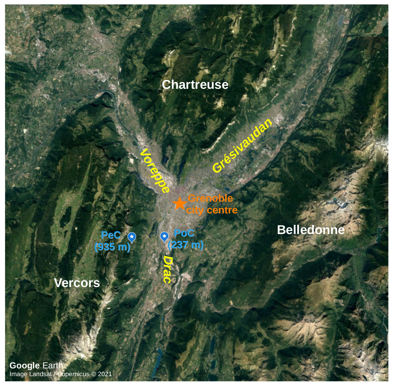
Figure 1 Satellite view of the Y-shaped Grenoble valley system from © Google Earth. The location of the weather stations is indicated in blue; the names of the valleys and mountain chains are indicated in yellow and white, respectively.

The city of Grenoble experiences poor air quality in winter when PCAPs form and ventilation of pollutants, mainly from wood combustion and traffic, is limited. It was shown by Largeron and Staquet (2016b), when analysing nine PCAPs of the winter of 2006–2007, that these PCAPs display characteristics (intensity and height) comparable to those of valleys in the Rocky Mountains documented by Whiteman et al. (1999b).

Several ground-based automatic weather stations are installed in the Grenoble valleys, operated by the air quality agency of the région Auvergne Rhône-Alpes (Atmo AuRA) and by the French weather forecast service (Météo-France). Measurements are air temperature at 2 m from the ground (T_2 m) and wind speed at 10 m, with hourly frequency. In this paper, temporal series of T_2 m recorded at two stations located at different altitudes are used to derive an indicator of the stability of the boundary layer when a cold-air pool forms (see Sect. 3). The two stations are Pont de Claix (PoC) at 237 m a.s.l. and Peuil de Claix (PeC) at 935 m a.s.l. (Fig. 1). It was shown in Largeron and Staquet (2016a) that the temperature field is nearly homogeneous horizontally during inversion periods; thus, a vertical gradient can be derived from stations located at different horizontal positions in the valley.

2.2 The model chain

In this study, three different numerical models are used. The outputs of a GCM at a resolution of ∼100 km are dynamically downscaled with a RCM at a resolution of 7 km over the Alps. The latter data set is further dynamically downscaled with a third atmospheric model at a high resolution (about 100 m) to investigate the atmospheric circulation in the Grenoble boundary layer. The latter simulations are relatively short (about one week long) because of their high computing time. The details of these three atmospheric models are described below. The notation “A ← B” indicates that the model A is forced by the model B, and the model chain is denoted as A ← B ← C.

2.2.1 The MPI-ESM1.2-HR GCM

The Max Planck Institute Earth System Model version 1.2 – Higher Resolution (MPI-ESM1.2-HR) is a coupled GCM (Müller et al., 2018). This model was run with a 100 km resolution (in the atmosphere) within the Coupled Model Intercomparison Project – Phase 6 (CMIP6; Eyring et al., 2016), providing both historical simulations from 1850 and future projections based on different SSP–RCP scenarios (O'Neill et al., 2016). MPI-ESM1.2-HR was chosen for this study because it is one of the GCMs showing a limited bias over the Europe–North Atlantic area (Cannon, 2020; Fernandez-Granja et al., 2021). This GCM shows also a climate sensitivity (i.e. a temperature response to a doubling of carbon dioxide emissions) compatible with the observations (Mauritsen et al., 2019), while many other CMIP6 models have instead a climate sensitivity that is too large (Zelinka et al., 2020). Moreover, MPI-ESM1.2-HR captures well anticyclonic episodes associated with European atmospheric blocking, as shown in Bacer et al. (2022).

Ensemble member experiments have been produced with MPI-ESM1.2-HR within the CMIP6, but due to the large computational cost of the dynamical downscaling, we consider only the first member (r1i1p1f1, where r is initial conditions, i is initialization method, p is physical scheme, and f is forcing configuration). The experiments used in this paper are a historical run (Jungclaus et al., 2019) and two future runs based on SSP2–4.5 (Schupfner et al., 2020a) and SSP5–8.5 (Schupfner et al., 2020b). We will refer to the MPI-ESM1.2-HR model simply as “MPI” for conciseness and to the three experiments over their respective periods as MPI_HIST, MPI_SSP2, and MPI_SSP5.

2.2.2 The MAR RCM

The RCM used in the present study is the Modèle Atmosphérique Régional (MAR; Gallée and Schayes, 1994; Gallée et al., 2005).

A brief overview of the MAR model

MAR is a hydrostatic, primitive equation model with constant sigma coordinates on the vertical axis. MAR has been developed in particular for polar regions (e.g. Gallée et al., 1996; Fettweis et al., 2017) including a multi-layer snow cover model (Brun et al., 1992) with prognostic equations for snow density, temperature, water content, and albedo that allow an estimation of the surface mass balance of ice sheets and a realistic representation of snow-covered area. MAR has also been used to downscale atmospheric reanalysis in high mountain areas, over the Himalayas (Ménégoz et al., 2013) and over the Alps (Ménégoz et al., 2020), and has been shown to provide an accurate estimation of precipitation rates including snowfall rates.

In the Alpine region, MAR is used with a 7 km resolution, which was chosen as a trade off between (i) the minimum resolution compatible with the hydrostatic approximation and the activation of the convective scheme and (ii) an accurate representation of the alpine topography and the atmospheric variables at different elevated areas. In winter, the model shows a fairly good agreement at intermediate elevations but presents a warm bias close to the surface (of about 2.5 ^∘C) and a cold bias at higher elevations, around 3000 m a.s.l. (Beaumet et al., 2021).

The MAR model in the present study

The version 3.9 of MAR is used to downscale the outputs of MPI in the three experiments mentioned above, MAR ← MPI_HIST (1981–2014), MAR ← MPI_SSP2 (2015–2100), and MAR ← MPI_SSP5 (2015–2100), for a domain extending from 1.5 to 18.5^∘ E and 41.5 to 49.5^∘ N (Fig. 2a). A spin-up of 1 year is required for the MAR experiments to ensure an equilibrium of the soil hydrothermal regime.

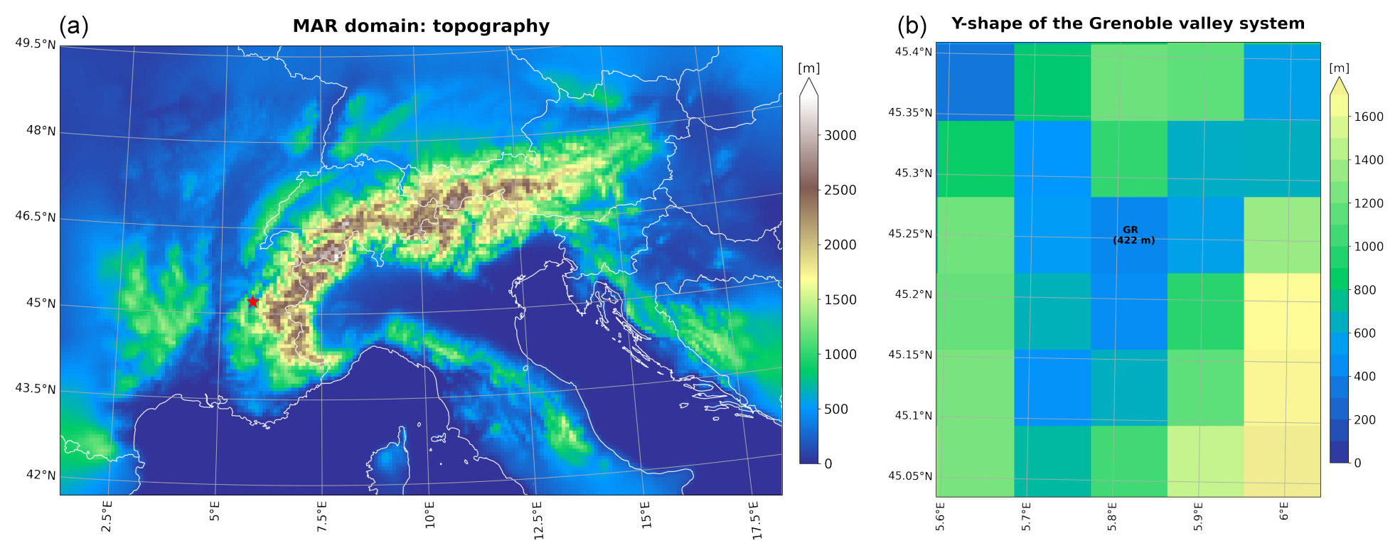
Figure 2 MAR domain with horizontal resolution of 7 km × 7 km (a); the red star indicates the location of Grenoble. Representation of the Y-shaped Grenoble valley system in MAR (b); the grid box labelled with GR is in the centre of the Grenoble basin and stands at the location of the Grenoble city, with altitude 422 m a.s.l.

The 7 km resolution smoothes the topography, which reaches a maximum altitude of 3500 m a.s.l. over the western Alps (Fig. 2a), while the highest summit (Mont Blanc) peaks at 4808 m. Regarding the representation of the Grenoble valley system, the surrounding summits reach at most 1700 m a.s.l. in Belledonne and 1200 m a.s.l. in Vercors and Chartreuse. Nevertheless, this resolution allows for a good representation of the Y-shape of the Grenoble valley system (Fig. 2b). As for Grenoble basin, the lowest altitude is 422 m a.s.l., i.e. about 200 m higher than the real altitude. The grid box in the centre of the basin, representative for the Grenoble city centre, is labelled with “GR” in Fig. 2b.

The vertical resolution is distributed through 24 levels, from the surface to 0.1 hPa. The outputs of the three experiments MAR ← MPI_HIST, MAR ← MPI_SSP2, and MAR ← MPI_SSP5 are available with daily resolution at different elevations (2, 10, 50, 100 m a.s.l.) and pressure levels (925, 850, 800, 700, 600, 500, 200 hPa). A data set for a limited number of variables and levels is available online (see “Data availability” at the end of this paper).

These daily outputs are used to identify PCAP episodes during the 21st century in Sect. 2.3.1 and to analyse the trends of the PCAP characteristics in Sect. 4. Experiments MAR ← MPI_HIST and MAR ← MPI_SSP5 are used to laterally force the third atmospheric model applied at high resolution; in this case, MAR is rerun saving hourly data distributed on 36 levels for the period of the selected PCAPs (more details on the MAR downscaling are provided in the Supplement).

2.2.3 The WRF model

The Weather Research and Forecasting (WRF) model is a state-of-the-art atmospheric modelling system designed for both meteorological research and numerical weather prediction. It is a fully compressible, non-hydrostatic model with a terrain-following, hybrid sigma–pressure vertical coordinate and the Arakawa-C grid staggering. The dynamical solver is the Advanced Research WRF (ARW). A detailed description of the model can be found in Skamarock et al. (2019). In the present work, version 4.1 is used, with the third-order Runge–Kutta time integration scheme and a fifth-order weighted essentially non-oscillatory (WENO) scheme with a positive definite filter for the advection terms. The model topography is based on the NASA Shuttle Radar Topography Mission (SRTM) digital elevation (version 4) with a resolution of 3 arcsec (i.e. approx. 90 m).

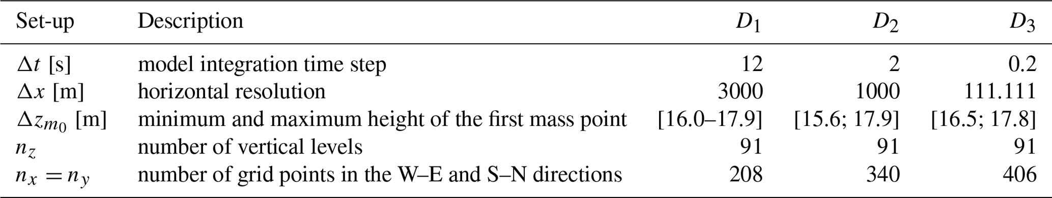
Sub-kilometre simulations with WRF have been performed for worldwide mountain valleys, e.g. the Salt Lake Valley at 250 m of resolution in the USA (Crosman and Horel, 2017). In Europe, alpine valleys such as the Bolzano basin (300 m; Tomasi et al., 2019), the Passy valley (111 m; Arduini et al., 2020; Quimbayo-Duarte et al., 2021), and the Inn valley (40 m; Umek et al., 2021) have been addressed. In this study, thanks to the definition of three online one-way nested domains (Fig. 3a), a resolution of 111 m is reached in the innermost domain covering the Grenoble valleys (Fig. 3b). Table 1 provides the details of spatial and temporal resolutions in each domain. Along the vertical, 91 model levels are defined up to 50 hPa (approx. 19 km a.s.l.). The thickness of the vertical model layers (Δz) increases approximately linearly in the first 50 layers before being stretched; the first 1000 m a.g.l. are discretized into 22 model levels, with the first mass point being located at about 17 m above the surface.

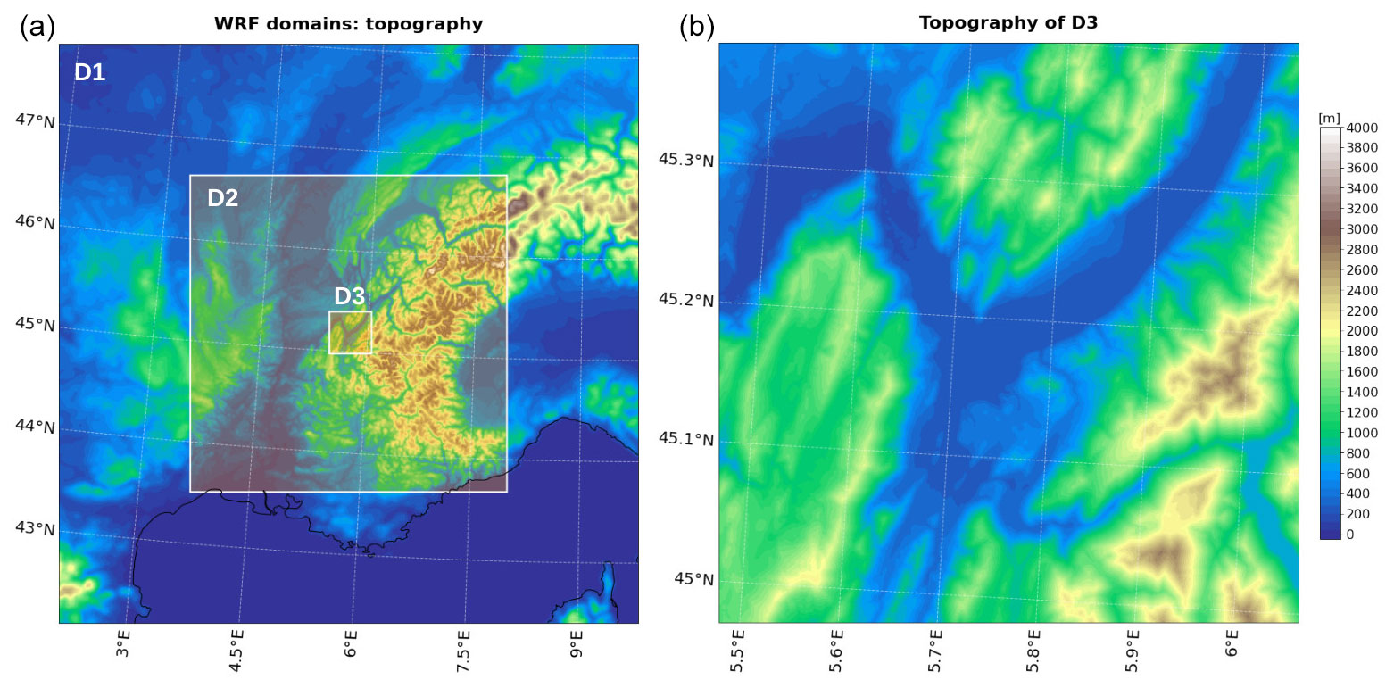
Figure 3 Topography in the three nested WRF domains (a) and in the innermost domain, D₃, with horizontal resolution 111 m × 111 m (b).

Table 1 Numerical parameters of the WRF simulations. D₁, D₂, and D₃ are three one-way nested domains.

The presence of steep slopes can generate numerical instabilities, even for high vertical resolution (see e.g. Connolly et al., 2021, for a discussion). To prevent these instabilities, a smoothing algorithm is applied to the topography of the innermost domain based on an optimization method in which the maximum slope angle is prescribed (Le Bouëdec et al., 2023). The latter angle is set to 28^∘ in the present work. For that angle, the smoothing procedure affects mainly the highest peaks, in the Belledonne chain in particular; the lowest parts of the valley slopes and the valley floors are only moderately or not affected. As discussed in Le Bouëdec et al. (2023), quite remarkably, the atmospheric circulation within a cold-air pool is found similar to the case of a maximum slope angle of 42^∘.

Since an accurate land use description is also important to correctly resolve the valley winds (Schmidli et al., 2018), the updated and high-resolution Corine Land Cover (CLC2018) data set with a horizontal resolution of 100 m is used. Land surface processes are modelled using the Noah land surface model (Chen and Dudhia, 2001), with four soil layers, and the Monin–Obukhov similarity theory (Jiménez et al., 2012) is used to couple the land surface to the atmosphere. Slope effects on radiation and the topographic shading are also considered.

For the two outermost domains the planetary boundary layer (PBL) is parameterized with the Yonsei University (YSU) scheme (Hong et al., 2006). For the higher-resolution simulations in the innermost domain, a three-dimensional turbulent kinetic energy (TKE) 1.5-order closure scheme is used (and no PBL scheme).

The WRF←MAR ← MPI model chain has been designed to simulate PCAP episodes during past and future climate (the dynamical downscaling of MAR with WRF is described in the Supplement). In particular, two WRF simulations have been run to describe one PCAP in the past and one around the middle of the 21st century. The identification and the selection of the episodes is described in Sect. 2.3.2. The WRF simulations are 5 d long, after a spin-up time of 1 d.

2.3 Detection of PCAPs

2.3.1 Identification of PCAPs from MAR ← MPI over the 21st century

In order to detect PCAP episodes in the Grenoble valley system during winter, we rely on the methodology proposed by Largeron and Staquet (2016a). These authors study persistent cold-air pools in the Grenoble valley boundary layer during the winter of 2006–2007. Winter encompasses the months from November to March and is denoted as NDJFM in their paper, and we adopt here the same definition and notation. Largeron and Staquet (2016a) use hourly temperature measurements recorded by meteorological stations located in the Grenoble valleys at different elevations and define PCAPs as periods during which the 24 h running mean of the ratio ($\mathrm{\Delta }T/\mathrm{\Delta }z$) is above the winter average, close to −3 K km⁻¹, for at least 3 d. By assuming horizontal homogeneity of temperature within the valleys, $\mathrm{\Delta }T/\mathrm{\Delta }z$ is defined as the ratio of the T_2 m difference between one station at high elevation and one station at low elevation and the difference in altitude of the two stations. Such a ratio is shown to be a good indicator of the stability of the atmosphere when a PCAP occurs (Largeron and Staquet, 2016a).

Since long-term MAR outputs are daily means and temperature at high elevation is available only at specific pressure levels (this is common in RCMs and GCMs), we adapt the method described above to our data set. We observe that the mean heights of the 925 and 850 hPa levels for the past 30 years (1981–2010) are equal to 787±91 and 1472±95 m a.s.l., respectively. The 850 hPa level is on average higher than Vercors and Chartreuse in MAR (Fig. 2b), while a PCAP height is usually close to the mean height of the mountains surrounding the valley (Whiteman, 1982; Largeron and Staquet, 2016b; Rasilla et al., 2022). On the contrary, the 925 hPa level should always be below the PCAP top observed in Grenoble. Since the temperature profile is approximately linear during inversions (Whiteman, 1982; Largeron and Staquet, 2016a), this level is chosen to compute the vertical temperature gradient modelled by MAR, which we assume to be representative of the entire PCAP height. Therefore, the modelled $\mathrm{\Delta }T/\mathrm{\Delta }z$ is defined as

$$\begin{array}{}\text{(1)}& (\mathrm{\Delta }T/\mathrm{\Delta }z{)}_{\mathrm{MAR}}={\displaystyle \frac{T_{\mathrm{925}\mathrm{hPa}}-T_{\mathrm{2}\mathrm{m}}}{Z_{\mathrm{925}\mathrm{hPa}}-z_{\mathrm{2}\mathrm{m}}}},\end{array}$$

where T_925 hPa is the temperature at 925 hPa, Z_925 hPa is the geopotential height at 925 hPa, and z_2 m is the altitude at 2 m a.g.l. $(\mathrm{\Delta }T/\mathrm{\Delta }z{)}_{\mathrm{MAR}}$ is computed at the GR grid box; hence z_2 m=424 m a.s.l.

PCAP episodes are identified with the following criterion:

$$\begin{array}{}\text{(2)}& \begin{array}{rl}(\mathrm{\Delta }T/\mathrm{\Delta }z{)}_{\mathrm{MAR}}>& {〈(\mathrm{\Delta }T/\mathrm{\Delta }z{)}_{\mathrm{MAR}}〉}_{\mathrm{30}\mathrm{winters}}^{\mathrm{HIST}}\\ & \mathrm{for}\mathrm{at}\mathrm{least}\mathrm{5}\mathrm{consecutive}\mathrm{days},\end{array}\end{array}$$

where ${〈(\mathrm{\Delta }T/\mathrm{\Delta }z{)}_{\mathrm{MAR}}〉}_{\mathrm{30}\mathrm{winters}}^{\mathrm{HIST}}$ is the winter average computed over 30 years (1981–2010) with MAR ← MPI_HIST, rounded to −3 K km⁻¹. This value is fully consistent with the winter average computed from the observations over 30 years (1985–2014) (see Sect. 3). Also, it is in agreement with Largeron and Staquet (2016a), who considered only one winter of observations, and close to Le Bouëdec (2021) (−2.5 K km⁻¹), who considered six winters of observations. Note that in the two latter references, the highest elevation station to compute the temperature gradient is at a higher altitude than PeC, about 1700 m.

A similar method is used by Iacobellis et al. (2009) to detect thermal inversions in California. These authors consider the temperature at 850 hPa and detect inversions if a ratio similar to Eq. (1) is greater than zero. By applying the same relation and condition for the Po Valley basin, (Caserini et al., 2017) obtain a strong underestimation of inversion frequency with the regional climate model they consider. Largeron and Staquet (2016a), who tested different thresholds, also find that the condition “greater than zero” is too restrictive as too few PCAP episodes are detected. This discussion stresses the importance of testing and choosing the best threshold for the inversion detection.

In this work, PCAPs are identified for the entire 21st century, from 1981 until 2100, using MAR ← MPI_HIST, MAR ← MPI_SSP2, and MAR ← MPI_SSP5.

2.3.2 Selection of two PCAP episodes to be simulated with WRF in the past and around 2050

The careful selection of two PCAPs, one in the past and one around 2050, to be simulated with WRF is an essential step to allow a meaningful comparison of the two episodes (see Sect. 5). Therefore, criteria are defined here in order to select two PCAPs that present common characteristics.

First, the episodes must be associated with a similar synoptic situation. The sensitivity of thermal inversion formation to large-scale atmospheric circulation and their higher occurrence during an anticyclonic regime have indeed already been demonstrated, as stressed in the Introduction. Wintertime anticyclonic conditions over the Grenoble area can occur during the Scandinavian atmospheric blocking, when it expands southwards. In this work, atmospheric blocking episodes are identified by applying the so-called weather type decomposition (WTD), a methodology that classifies the atmospheric circulation into discrete weather regimes (Michelangeli et al., 1995). The WTD consists of two steps: the dimensional reduction of the data set via the principal component analysis (PCA) and the clustering via the k-means algorithm. The data set involves here daily anomalies of geopotential height at 500 hPa. In this work, the number of clusters (k) is set to 4 in order to detect the four well-known weather types of the Euro-Atlantic sector, positive and negative North Atlantic Oscillation, Atlantic ridge, and Scandinavian atmospheric blocking; anticyclonic episodes are then selected during Scandinavian blocking.

In the present work, the WTD and the identification of blocking episodes follow the methodology used in Bacer et al. (2022). We apply the WTD to the data sets produced by MPI_HIST over the period 1981–2014 and by MPI_SSP5 over two successive 30-year periods, 2015–2045 and 2035–2065. We next select the blocking episodes that are at least 10 d long and, among them, retain those satisfying the following criteria:

1. Since these episodes are centred over western or northern Europe, in order to consider anticyclonic conditions in Grenoble, only those days characterized by daily sea level pressure (SLP) higher than 1030 hPa in Grenoble are kept; this criterion is applied by using the temporal series of SLP extracted at the GR grid box of the MAR outputs.

2. Only those days with $(\mathrm{\Delta }T/\mathrm{\Delta }z{)}_{\mathrm{MAR}}>-\mathrm{3}$ K km⁻¹ in GR are considered.

3. Conditions 1 and  2 must be satisfied for at least 5 consecutive days to define a PCAP.

4. The PCAPs must occur during the same period of the year, so that the incident solar radiation, which drives the thermal forcings of the valley circulation, is comparable among the episodes.

In this work, we look for PCAPs preferably around the years 2000 and 2050, in order to consider one episode in the near past and one episode in the middle of the century. We find that only two episodes satisfy all criteria, one in 1988 (14–21 December 1988) and one in 2043 (4–15 December 2043), as visible in Fig. S1 in the Supplement. We decide to consider 5 d in the centre of the episodes for the WRF simulations; therefore, the dates of the two selected PCAP episodes are 16–20 December 1988 and 8–12 December 2043.

During both episodes, the daily blocking patterns show a strong positive geopotential anomaly centred over central Europe, extending to the Iberian Peninsula (Fig. S2). The winds at 500 hPa over south-eastern France are lower than 10 m s⁻¹ except during the first 2 d of the episode in 1988, when the winds are stronger. In particular, the atmospheric blocking is not well structured on the first day (16 December 1988) yet, and westerlies still cross France zonally; this will affect the structure of the thermal inversions formed in the Grenoble valleys during these days (see Sect. 5).

3 Reliability of MAR ← MPI to predict the stability of the valley atmosphere

Before analysing the PCAPs predicted by MAR in the future and downscaling MAR with WRF, an essential step is to check the reliability of MAR ← MPI in the past. For this purpose, the daily temperature gradient computed with MAR ←MPI_HIST (see definition Eq. 1) is compared with the observed vertical temperature gradient, noted $(\mathrm{\Delta }T/\mathrm{\Delta }z{)}_{\mathrm{obs}}$, during NDJFM over the period 1985–2014. This gradient is computed with daily means of T_2 m measured at the two weather stations presented in subsection 2.1 as

$$\begin{array}{}\text{(3)}& (\mathrm{\Delta }T/\mathrm{\Delta }z{)}_{\mathrm{obs}}=\left(T_{\mathrm{2}\mathrm{m}}^{\mathrm{PeC}}-T_{\mathrm{2}\mathrm{m}}^{\mathrm{PoC}}\right)/\left(z^{\mathrm{PeC}}-z^{\mathrm{PoC}}\right),\end{array}$$

with z being the altitude of the two stations (237 and 935 m a.s.l.).

Figure 4 displays the probability density functions (PDFs) of both data sets over the 30 winters of the 1985–2014 period, which contain 4447 d. The agreement between the PDFs is remarkable. The mean values are equal to −3.2 K km⁻¹ for the model results and to −3.1 K km⁻¹ for the observations. The winter days characterized by $\mathrm{\Delta }T/\mathrm{\Delta }z>-\mathrm{3}$ K km⁻¹ represent 43.5 % of the data set according to MAR and 41.6 % according to the observations, which corresponds to a difference of about 80 d. The MAR distribution is slightly shifted to the right with respect to the observations until about 4 K km⁻¹ but presents a shorter tail for higher values (the number of winter days with $\mathrm{\Delta }T/\mathrm{\Delta }z>\mathrm{4}$ K km⁻¹ represents 2.2 % of the MAR data and 5.7 % of the observations). This underestimation of the model could be due to the warmer bias of MAR close to the ground (see Sect. 2.2.2), which leads MAR to slightly underestimate the atmospheric stability in the valley. Moreover, it should be reminded that the level of the valley bottom in MAR is about 200 m higher than the actual topography (see Sect. 2.2.2); during PCAP days (when temperature increases with altitude), this could also cause an overestimation of the modelled T_2 m, contributing to reduce $(\mathrm{\Delta }T/\mathrm{\Delta }z{)}_{\mathrm{MAR}}$.

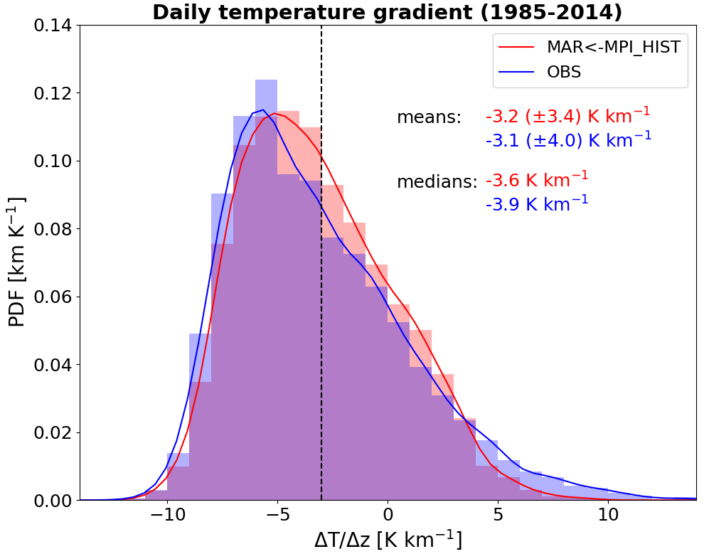
Figure 4 Normalized probability density functions (PDFs) of daily temperature gradient computed with MAR ← MPI_HIST, i.e. $(\mathrm{\Delta }T/\mathrm{\Delta }z{)}_{\mathrm{MAR}}$ defined by Eq. (1) (red), and observations, i.e. $(\mathrm{\Delta }T/\mathrm{\Delta }z{)}_{\mathrm{obs}}$ defined by Eq. (3) (blue), over 30 years (1985–2014) during winter (NDJFM). The vertical line indicates the value −3 K km⁻¹ (i.e. the threshold used to identify the PCAP episodes); the standard deviation is in parentheses.

A further comparison between model results and observations is performed by considering only the PCAP episodes (defined by criterion Eq. 2) during the same 30 winters. The total number of days belonging to PCAPs derived from MAR is 886, while the one derived from the observations is 1040. Since the number of winter days with $\mathrm{\Delta }T/\mathrm{\Delta }z>-\mathrm{3}$ K km⁻¹ is similar as indicated above, we deduce that several of these days in MAR are not consecutive and, therefore, do not belong to a PCAP episode. The total number of episodes, 119 according to MAR and 91 according to the observations, indeed indicates that MAR simulates shorter episodes. This is confirmed by the PDF of the duration of the PCAPs in Fig. 5a. Since this analysis concerns the right tails of the PDFs in Fig.4, only the median values are computed. The simulated and observed PCAPs are finally compared in terms of intensity, defined as the temporal mean of the daily vertical temperature gradients over the duration of the PCAP. As expected from Fig. 4, the modelled PCAPs tend to be less intense than the observed ones, with an intensity median smaller by 0.2 K km⁻¹ (Fig. 5b).

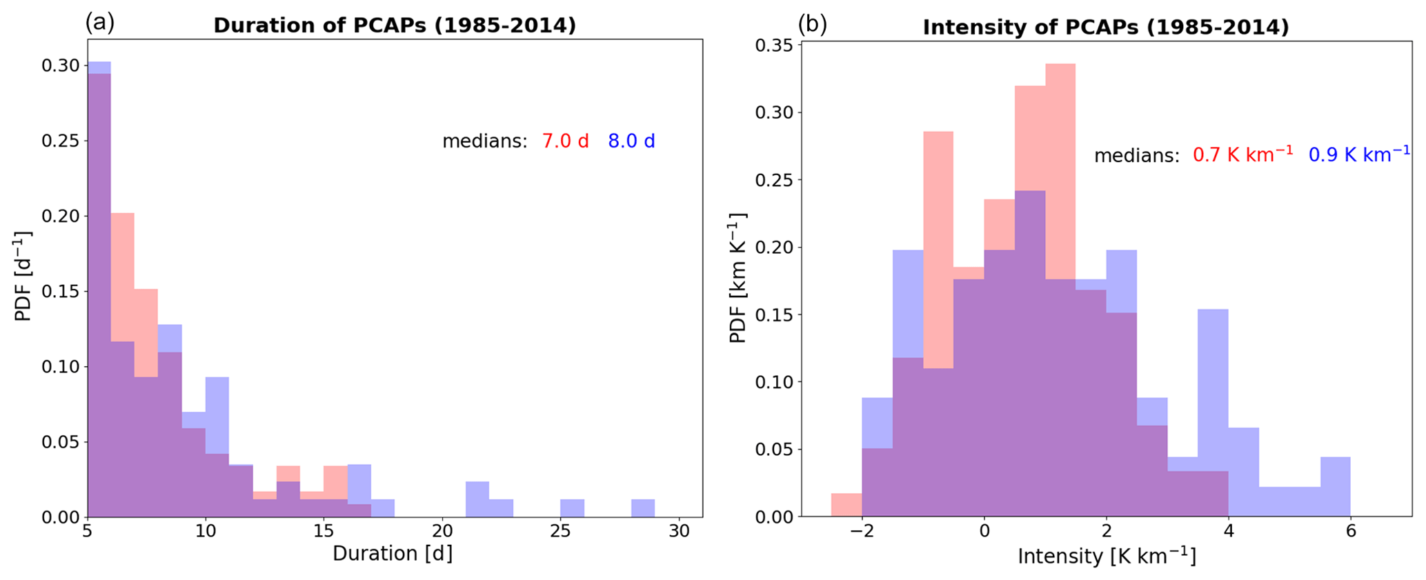
Figure 5 PDF of duration (a) and intensity (b) of the PCAP episodes identified over 30 years (1985–2014) during winter with MAR ← MAR_HIST (red) and observations (blue).

Overall, we can conclude that MAR ← MPI_HIST reproduces well the vertical temperature gradient in the Grenoble basin. Therefore, MAR ← MPI outputs can be reasonably used to (i) analyse future PCAPs and (ii) force WRF. Moreover, we prove that definition (Eq. 1), with temperature at 925 hPa, is a good alternative to compute the vertical temperature gradient in the absence of temperature at specific altitudes or vertical temperature profiles.

4 Impact of climate change on PCAPs in the Grenoble basin over the 21st century

4.1 Trends of $(\mathrm{\Delta }T/\mathrm{\Delta }z{)}_{\mathrm{MAR}}$ over the 21st century

We analyse the impact of climate change on the vertical temperature gradient in the centre of the Grenoble valleys (i.e. in GR) over the winters during the 21st century. We simplify the notation by referring to the 120-year-long simulations from 1981 to 2100 as MAR ← MPI_SSP2 and MAR ← MPI_SSP5 (thus abandoning MAR ← MPI_HIST as this historical run is common to both periods).

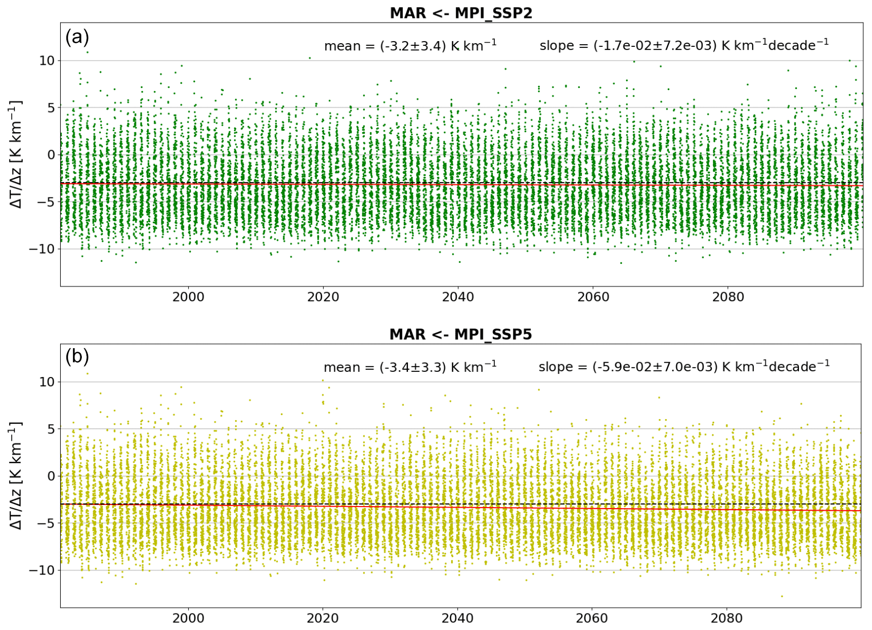
Figure 6 Temporal series of daily winter $(\mathrm{\Delta }T/\mathrm{\Delta }z{)}_{\mathrm{MAR}}$ for MAR ← MPI_SSP2 (a) and MAR ← MPI_SSP5 (b). The horizontal dashed black line refers to the value $\mathrm{\Delta }T/\mathrm{\Delta }z=-\mathrm{3}$ K km⁻¹. The red line is the trend computed as linear regression (which is statistically significant at 95 %, with p value equal to 0.017, for SSP2–4.5 and at 99 %, with p value of the order of 10⁻¹⁷, for SSP5–8.5). The mean and the slope of the trend (± standard deviation) refer to the entire time series (i.e. 120 winters).

The temporal series of $(\mathrm{\Delta }T/\mathrm{\Delta }z{)}_{\mathrm{MAR}}$ during this period are presented in Fig. 6. Under both future scenarios, the series have a temporal mean of about −3 K km⁻¹, with a standard deviation also equal to about −3 K km⁻¹. They both present a statistically significant negative trend indicating a decreasing atmospheric stability, with the slope of the trend being larger for MAR ← MPI_SSP5 than for MAR ← MPI_SSP2 ($-\mathrm{0.059}\pm \mathrm{0.007}$ K km⁻¹ per decade versus $-\mathrm{0.017}\pm \mathrm{0.007}$ K km⁻¹ per decade), consistent with global warming being larger for SSP5–8.5 than for SSP2–4.5. The analysis of $(\mathrm{\Delta }T/\mathrm{\Delta }z{)}_{\mathrm{MAR}}$ distributions over 30 years around 2000, 2050, and 2085 highlights a gradual decrease of strong inversion days in the worst-case scenario (Fig. S3, right panel).

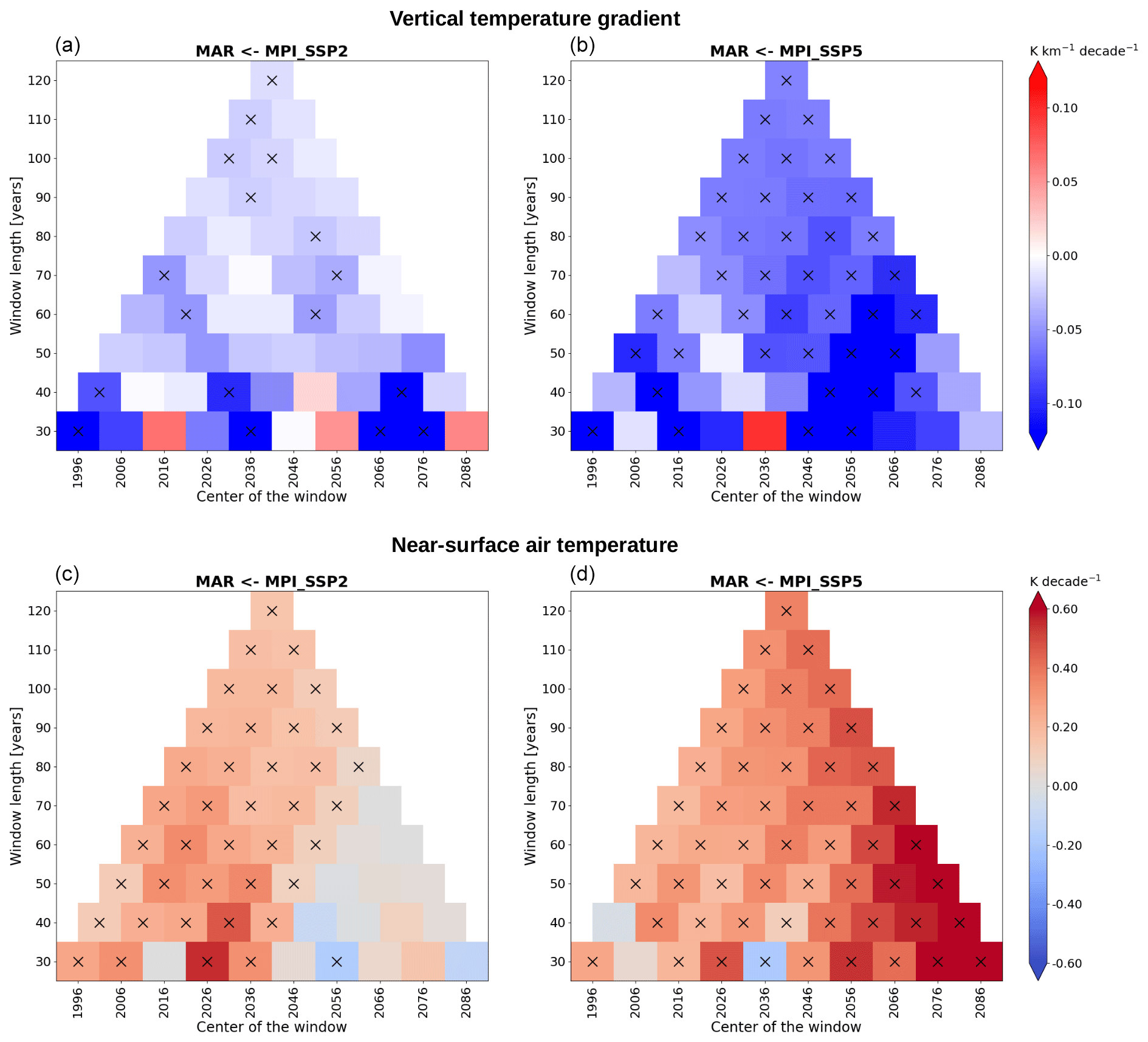
Figure 7 Slope coefficients of the trends computed in sliding windows of variable length for $(\mathrm{\Delta }T/\mathrm{\Delta }z{)}_{\mathrm{MAR}}$ (a, b) and T_2 m (c, d) for MAR ← MPI_SSP2 and MAR ← MPI_SSP5. The windows have a minimal length of 30 years; they slide with a step of 10 years throughout the entire time series (1981–2100). The windows also have a variable length, increasing by 10 years until they reach the maximum length equal to the length of the entire time series. The years that are central in the windows are on the x axis; the length of the windows is on the y axis. The black crosses mark trends that are statistically significant at 95 %.

Trends of the $(\mathrm{\Delta }T/\mathrm{\Delta }z{)}_{\mathrm{MAR}}$ temporal series obtained with MAR ← MPI_SSP2 and MAR ← MPI_SSP5 are also computed in sliding windows with a 10-year step and of variable length, from 30 years to the length of the entire time series (Fig. 7a and b). In the past, three windows can be considered: 1981–2010 and 1991–2020 (30 years long) and 1981–2020 (40 years long). For these periods, the vertical temperature gradient trends are negative, although not always statistically significant. Figure 7a  and b confirm the long-term tendency of the vertical temperature gradient to decrease, thereby reducing the atmospheric stability in the valley, especially for SSP5–8.5. Under the latter scenario indeed, the trends are almost always negative whatever the window and always statistically significant with windows longer than 70 years. The slope coefficients are larger in the second half of the century, with values up to $-\mathrm{0.208}\pm \mathrm{0.036}$ K km⁻¹ per decade with windows of 40 years. With respect to this scenario, the trends in MAR ← MPI_SSP2 are less often statistically significant; the slope coefficients are smaller and always negative with windows longer than 40 years.

The behaviour of $(\mathrm{\Delta }T/\mathrm{\Delta }z{)}_{\mathrm{MAR}}$ is further analysed by comparing the time series of T_2 m to those at mid-altitudes in the free air. The time series of T_2 m are displayed in Fig. S4 for the two scenarios. As expected, the near-surface temperature is projected to increase, especially for the worst-case scenario. The trends computed for T_2 m in the same sliding windows as for $(\mathrm{\Delta }T/\mathrm{\Delta }z{)}_{\mathrm{MAR}}$ are displayed in Fig. 7c and d. This figure shows that T_2 m increases until the middle of the century under the SSP2–4.5 scenario, while the increasing trend persists until the end of the century under SSP5–8.5.

The temperature at higher altitudes in the free air is available on pressure surfaces (i.e. not at fixed altitudes) from the MAR data. The time-averaged value of Z_925 hPa is 794 m ± 91.6 m a.s.l., which makes T_925hPa a proxy for the temperature at about 800 m a.s.l. The time series of T_925 hPa in GR are displayed in Fig. S5 for the two scenarios. The trends are statistically significant for both scenarios; they are positive and of lower value than the T_2 m trends. For SSP5–8.5, for instance, the trends are equal to (0.37±0.01) K per decade for T_2 m and to (0.34±0.01) K per decade for T_925 hPa. The difference between these trends is very weak, but it is quantitatively consistent with the trend of $(\mathrm{\Delta }T/\mathrm{\Delta }z{)}_{\mathrm{MAR}}$. (Similar results are obtained when the time series of T_850 hPa is considered: the trend is equal to (0.14±0.01) K per decade for SSP2–4.5 and (0.33±0.01) K per decade for SSP5–8.5.) This result shows that the decaying trend of $(\mathrm{\Delta }T/\mathrm{\Delta }z{)}_{\mathrm{MAR}}$ over the century is due to the fact that air temperature close to the surface increases more than in the free atmosphere at mid-altitude in the valley. This higher increase of T_2 m over the century may be related to the increase of the specific humidity (which is a greenhouse gas) at the same location (see Fig. S6) and the consequent reduction of the radiative cooling of the ground (Philipona, 2013).

4.2 Characteristics of PCAP episodes over the 21st century

We now investigate the impact of climate change on the characteristics of the PCAP episodes identified over the 21st century (see criterion Eq. 2). We focus on the intensity (i.e. the temporal mean of the daily vertical temperature gradients over the duration of the PCAP), the duration, and the frequency (i.e. the number of episodes in a given time period). Figure 8 displays the temporal series of these quantities per year, i.e. the annual mean intensities, mean durations, and frequencies, where “annual” always refers to wintertime. The time series of intensity and duration are displayed in Fig. S7 for all identified PCAPs. All time series show a large interannual variability (as in Yu et al., 2017). As expected from the previous analysis, PCAPs will be less intense for the worst-case scenario, changing from a 30-year mean of 0.62±1.26 K km⁻¹ around the year 2000 to a 30-year mean of 0.27±1.06 K km⁻¹ at the end of the century (Table 2). Also in this case, the decrease is more evident in the second half of the century (Table 2 and Fig. S7). On the contrary, PCAP intensities for the SSP2–4.5 scenario do not present any significant change, and extreme episodes occur throughout the century (Table 2 and Fig. S7).

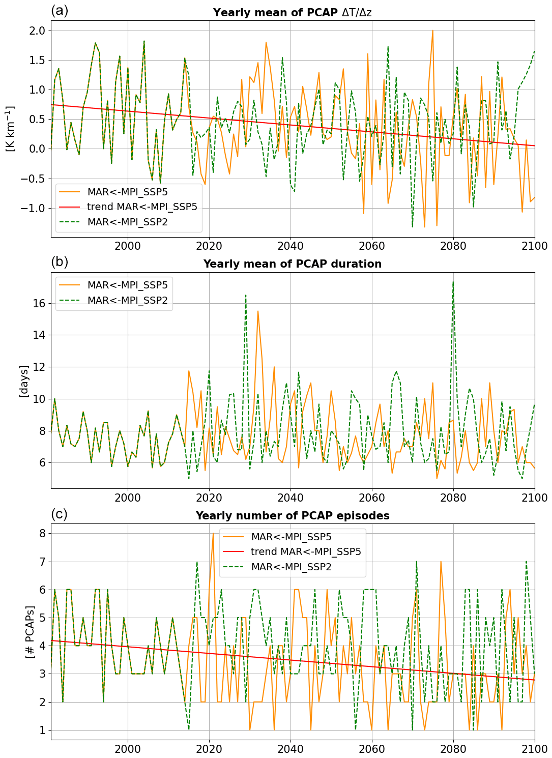
Figure 8 Temporal series of annual means of PCAP intensities (a), annual means of PCAP durations (b), and annual number of PCAP episodes (c). The trends in red (computed as linear regressions) are statistically significant at 99 %, with p value equal to 0.002 and slope ($-\mathrm{0.058}\pm \mathrm{0.019}$) K km⁻¹ per decade (a) and p value equal to 0.003 and slope ($-\mathrm{0.118}\pm \mathrm{0.039}$) number of PCAPs per decade (c).

Table 2 Mean values (± standard deviation and [minimum; maximum]) of intensity, duration, and number of the PCAP episodes occurring over 30-year periods (see also Fig. S7). The term “around 2000” refers to the 1985–2014 period, “around 2050” to the 2035–2064 period, and “around 2085” to the 2070–2099 period.

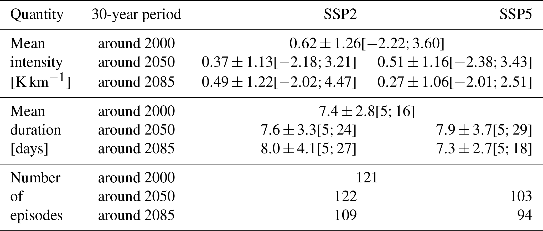
The annual mean PCAP duration (Fig. 8b) varies between 5 and 10 d during the historical period, while it can be longer in the future for both scenarios (up to 15 d under SSP2 and 17 d under SSP5), with no statistically significant trend. Considering all PCAPs occurring in periods of 30 years, the mean duration is between 7 and 8 d for both scenarios (Table 2).

The annual number of PCAPs (Fig. 8c) varies between 2 and 6 during the historical period and is comprised (almost always) between 1 and 7 during both future periods. More precisely, this quantity shows a statistically significant negative trend for the worst-case scenario only. This is evident also in Table 2, where the total number of episodes over a 30-year period decreases from 121 in the past to 94 at the end of the century. Since the PCAP duration remains essentially stable, this reduction implies that the annual number of PCAP days also tends to decrease.

5 Vertical structure of two PCAP episodes in the Grenoble valleys

The analysis now focuses on 5 d of two PCAP episodes (see Sect. 2.3.2 for the selection method of these episodes) that have been simulated at high resolution with the model chain WRF ← MAR ← MPI_SSP5 (see Sect. 2.2.3 for the WRF set-up). This 5 d period is in the middle of each PCAP episode, when the PCAP stability is largest. One episode occurs in the past (16–20 December 1988) and the other one in the future (8–12 December 2043). In the following, these 5 d periods are referred to as Ep1988 and Ep2043, respectively.

5.1 General features of the two PCAP episodes

An overview of the two episodes is provided in Fig. 9 through vertical profiles (up to 2000 m a.g.l.) of temperature and horizontal wind speed over the 5 selected days of each episode. These fields are averaged over the two main Grenoble valleys, Grésivaudan and Voreppe, and over the Grenoble basin (these areas are displayed in Fig. S8). The averaged profiles thus obtained are assumed to be representative of each valley section.

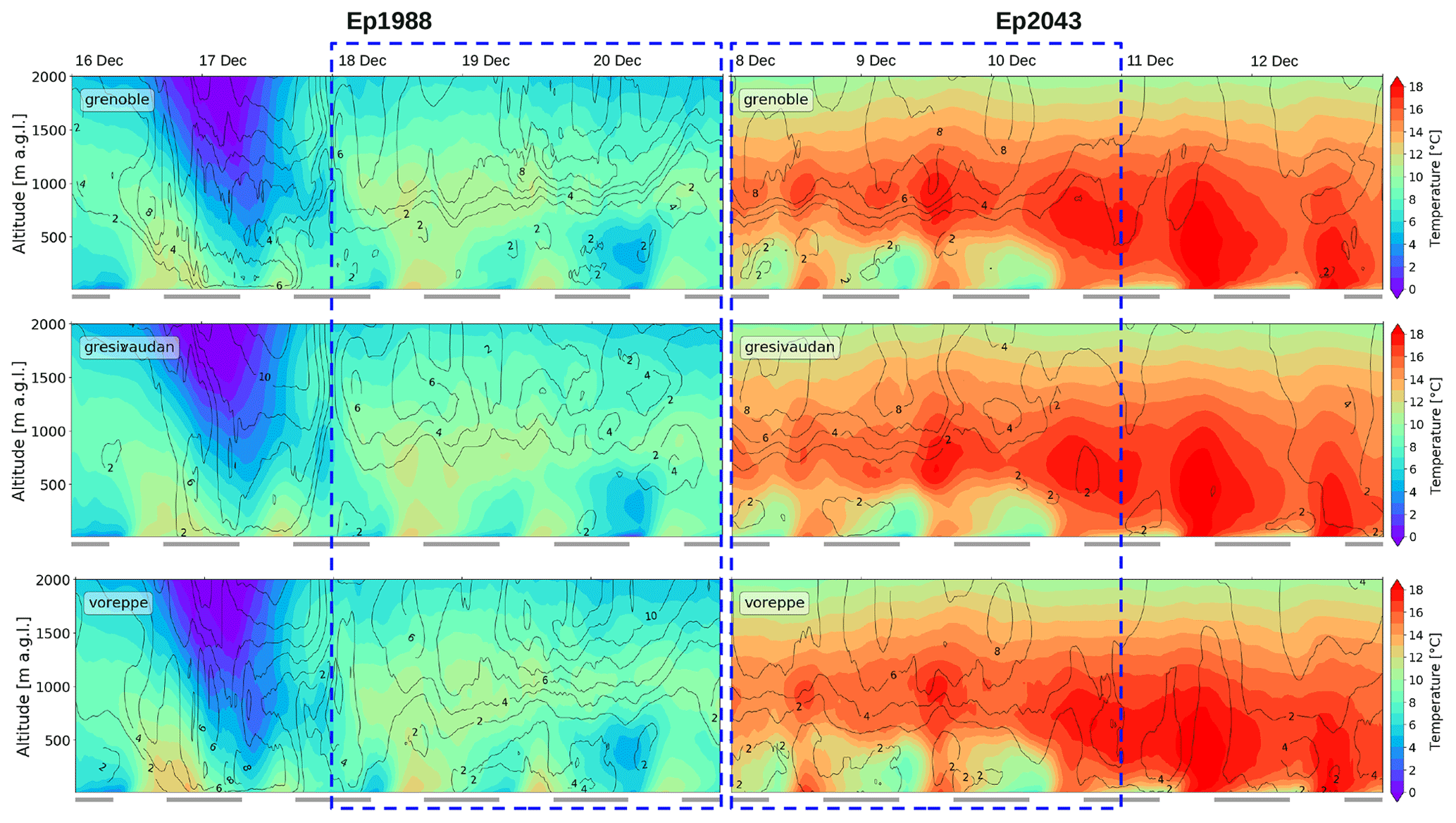
Figure 9 Vertical profiles of temperature (colour shading) and wind speed (black contours from 0 to 14 m s⁻¹, every 2 m s−1) as functions of time for Ep1988 and Ep2043. These quantities are spatially averaged over the Grenoble basin, Grésivaudan valley, and Voreppe valley (these areas are displayed in Fig. S8). The horizontal grey lines along the x axis indicate the nighttime period, between 17:00 and 07:00 UTC; the rectangles on the dashed blue line indicate the 3 selected days for each episode.

As shown in Fig. 9 the arrival of the anticyclone over Grenoble is associated with that of a warm air mass around 1000 m a.g.l., from 18 December in Ep1988 and from 8 December in Ep2043. This warm air layer persists at mid-altitude over the remaining days of the episode and maintains the thermal inversion.

The thermal inversion of Ep2043 is stronger than that of Ep1988. This is attested in Fig. S9, which displays the temperature and potential temperature profiles of each episode averaged over 3 d (see next section for the choice of these days). The vertical gradients of these profiles, which are positive in the cold-air pool (below about 800 m a.g.l.), are indeed stronger for Ep2043 than for Ep1988. This implies that the statistical trend observed over the century, indicating a slightly decreasing stability, is not recovered. There is not contradiction because only two (past and future) PCAP episodes are selected. This implies that some of the results inferred from this analysis, which aims at comparing the vertical structure of the future episode against that of the past one, will not apply to all PCAP episodes of the century.

The striking feature of Fig. 9 is the difference in temperature between the two episodes: Ep2043 is warmer than Ep1988 up to 2000 m a.g.l. Figure S9 helps quantifying this temperature difference: it is larger than about 4 K at all altitudes whatever the time of the day. This is consistent with the projection of T_2 m (Fig. S4, bottom panel) and T_925 hPa (Fig. S5, bottom panel), which display an increasing trend over the century for the SSP5–8.5 scenario. Around 800 m a.g.l., near the top of the cold-air pool, this temperature difference is even larger, 8 K or so, a value which depends upon the difference in stability between the two episodes.

The along-valley wind is very weak within the cold-air pool for both episodes, less than 2 m s⁻¹. It increases above for the two episodes, still remaining lower than ≃8 m s⁻¹, consistent with the synoptic regime being anticyclonic. Hence, as opposed to the temperature field, the atmospheric circulation in the cold-air pool of the Grenoble valleys appears to be similar in the two episodes (see also Fig. S10).

Although the 5 d of the PCAP episodes were carefully chosen (see the criteria discussed in Sect. 2.3.2) and were in the middle of an anticyclonic period, a cold air intrusion occurs during Ep1988: stronger winds and cold air enter in the valleys on 17 December 1988, perturbing the atmosphere. Note that this event could not be detected from the large-scale wind pattern at 500 hPa.

5.2 Height and strength of the two PCAP episodes

The three main characteristics of the PCAPs, atmospheric stability, inversion height, and inversion strength, are now considered for a more quantitative analysis.

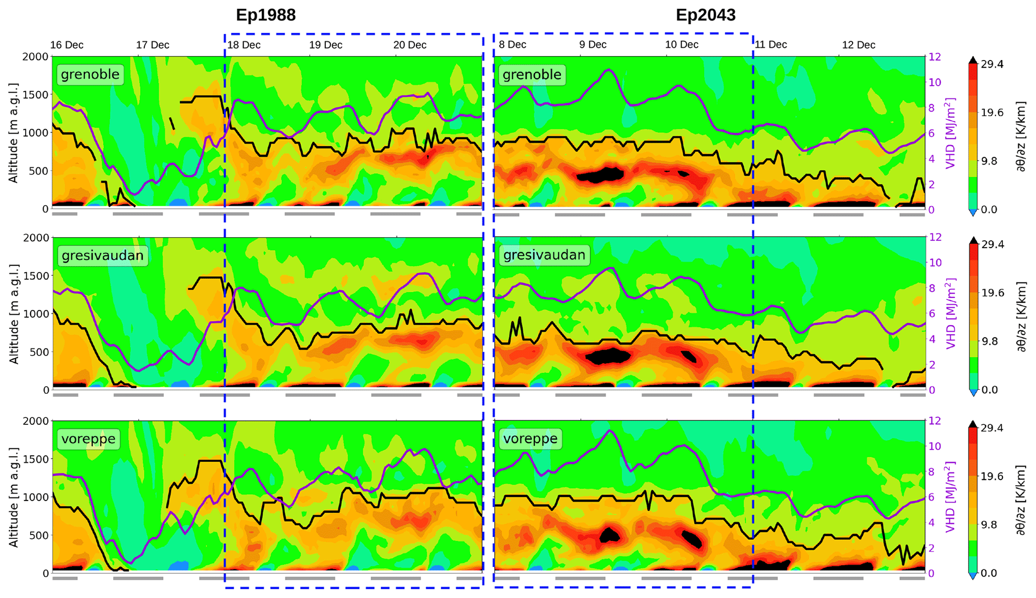
Figure 10 Vertical gradient of the potential temperature $\partial \mathit{\theta }/\partial z$ (colour shading), inversion height (black line, left y axis), and valley heat deficit, VHD (purple line, right y axis), for Ep1988 and Ep2043. These quantities are computed from the potential temperature, once temporally averaged (over 1 h) and spatially averaged over the Grenoble basin, Grésivaudan valley, and Voreppe valley (see Fig. S8). The horizontal grey segments along the x axis indicate the time between 17:00 and 07:00 UTC; the rectangles on the dashed blue line indicate the 3 selected days for each episode.

The atmospheric stability is now expressed in terms of the vertical gradient of potential temperature, $\partial \mathit{\theta }/\partial z$, with respect to the adiabatic lapse rate for dry atmosphere, Γ_d ($\simeq -\mathrm{9.8}$ K m⁻¹): $\partial \mathit{\theta }/\partial z>\left|{\mathrm{\Gamma }}_{\mathrm{d}}\right|$ is associated with an inversion, $\mathrm{0}<\partial \mathit{\theta }/\partial z<\left|{\mathrm{\Gamma }}_{\mathrm{d}}\right|$ to a moderately stable atmosphere, and $\partial \mathit{\theta }/\partial z<\mathrm{0}$ to an unstable atmosphere. The inversion height, denoted H_inv, is computed as the highest elevation, where $\partial \mathit{\theta }/\partial z>\left|{\mathrm{\Gamma }}_{\mathrm{d}}\right|$ below 1500 m a.g.l. (as in Largeron and Staquet, 2016a). The strength of the inversion is quantified by the valley heat deficit (VHD; Whiteman et al., 1999a):

$$\begin{array}{}\text{(4)}& \mathrm{VHD}=c_{\mathrm{p}}\underset{z_{\mathrm{0}}}{\overset{z_T}{\int }}\mathit{\rho }\left(z\right)\left[\mathit{\theta }\left(z_T\right)-\mathit{\theta }\left(z\right)\right]\mathrm{d}z\left[\mathrm{J}{\mathrm{m}}^{\mathrm{2}}\right],\end{array}$$

where c_p=1005 J K⁻¹ kg⁻¹ is the specific heat capacity of air at constant pressure and ρ is the air density; the lower bound z₀ is set to 0 (ground level) and the upper bound z_T is set to the maximum value among the six 95th percentiles of H_inv (one per episode and per area displayed in Fig. S8), leading to z_T=1050 m. The quantity VHD is the amount of heat per unit area necessary to bring the temperature gradient of the fluid column extending from z₀ to z_T to the dry adiabatic lapse rate; in other words, it is the energy required to fully mix this air column and destroy the inversion.

Figure 10 displays the temporal evolution of $\partial \mathit{\theta }/\partial z$, H_inv, and VHD, spatially averaged over the Grenoble basin, the Grésivaudan valley, and the Voreppe valley. The inversion in Ep1988 is temporarily disturbed and destroyed between the night of 17 December and the morning of 18 December (as previously observed in Fig. 9), while the inversion height in Ep2043 decays down to a few hundred metres above ground level from 10 December and is disturbed on 12 December. Therefore, we focus on the last 3 d (18–20 December) of Ep1988 and the first 3 d (8–10 December) of Ep2043 in the following analysis.

The $\partial \mathit{\theta }/\partial z$ values show that the atmosphere below the top of the cold-air pool is more stable in Ep2043 than in Ep1988, as already discussed in Sect. 5.1, with $\partial \mathit{\theta }/\partial z$ reaching values greater than 29.4 K km⁻¹ not only in the surface layer during nighttime but also in a layer around 500 m a.g.l. (where the temperature abruptly changes in Fig. 9). This difference in stratification between the two episodes is also attested in Fig. S9 (bottom row panels).

A specific feature of a PCAP episode is that H_inv is insensitive to the diurnal cycle. As noted in Sect. 2.3.1 the height of a PCAP is set by the mean height of the surrounding summits or plateaux (Whiteman, 1982). This is illustrated in Fig. 10 for both episodes. During daytime, the cold-air pool is eroded close to the surface by a shallow convective layer, of at most 50 m, while the atmosphere above remains stable. As a result, H_inv hardly varies between night and day. Figure 10 also shows that the inversion height is slightly lower in Ep2043 than in Ep1988 by about 100 m on average (see Table 3); these differences are however not significant due to the variability of the inversion height.

Table 3 Temporal mean (± standard deviation) of the inversion height and VHD computed over 3 d (18–20 December 1988 and 8–10 December 2043) and spatially averaged over the Grenoble basin, Grésivaudan valley, and Voreppe valley (see Fig. S8).

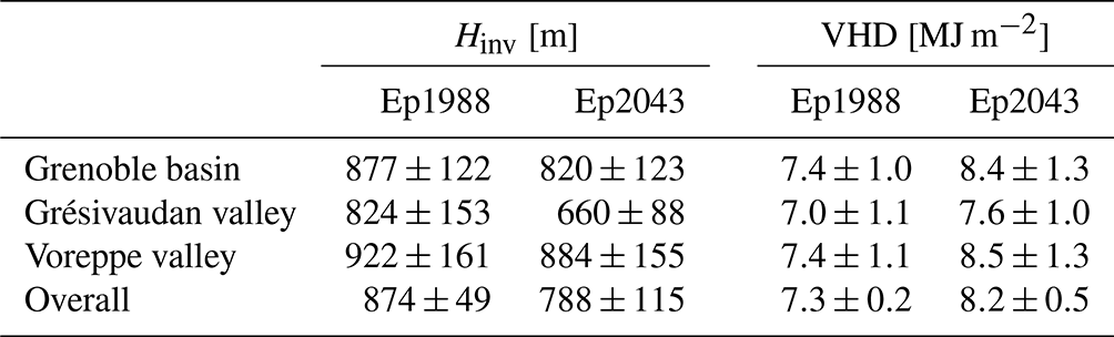
By contrast, the VHD displays a diurnal cycle, with local minima during daytime (when the cold-air pool is eroded from below) and local maxima during nighttime. When VHD is averaged over each episode, higher values are found for Ep2043 than for Ep1988 (see Table 3), consistent with the former PCAP being more stable than the latter. This range of values is of the same order of magnitude as those computed for real episodes (i.e. real-case simulations run with WRF forced by reanalysis): for the Grenoble valleys, values equal to 10–20 MJ m⁻² were found by Largeron and Staquet (2016b) for PCAPs of the 2006–2007 winter (with z_T=1500 m a.g.l.); for the Arve River valley (also in the French Alps), values equal to 8–12 MJ m⁻² were computed in Arduini et al. (2020) during a PCAP in February 2015 (with z_T≃1000 m a.g.l.).

The link between PCAP stability, height, and strength (VHD) can be qualitatively accounted for by noting that, when the potential temperature profile is linear, these three quantities are related by VHD=0.5ρc_pH_invΔθ, where Δθ is the potential temperature difference across the cold-air pool (Whiteman et al., 1999b).

6 Conclusions

We investigate the impact of climate change on persistent cold-air pools (PCAPs) in winter in the Grenoble valleys during the 21st century. For this purpose, two distinct analyses are carried out. We first perform a statistical analysis of PCAP characteristics over the century from data of a regional climate model. The vertical structure of two carefully selected PCAPs, one in the past and one around 2050, is next investigated using high-resolution simulations for the SSP5–8.5 scenario.

The statistical analysis of the PCAP characteristics relies on outputs of the regional climate model MAR forced by the general circulation model MPI (MAR ← MPI) from 1981 to 2100 for two different future scenarios, SSP2–4.5 and SSP5–8.5. We propose a simple methodology to identify PCAPs from the MAR data, which we validate against observations. This methodology consists in computing wintertime daily averaged vertical temperature gradients between the ground and the 925 hPa pressure level (i.e. about 800 m a.s.l.; see Sect. 2.3.1) assuming the temperature profile is linear during PCAP episodes and using a threshold lower than 0 to detect the inversions (see relation Eq. 2 for more details). As shown in the literature (e.g. Caserini et al., 2017), using a threshold equal to 0 leads to an underestimation of the number of PCAP episodes.

The statistical analysis of the wintertime vertical temperature gradients reveals a significant decreasing trend over the century for both SSP2–4.5 and SSP5–8.5. However, decay rates are very weak: 0.059 K km⁻¹ per decade for SSP5–8.5 and about 3.5 times lower for SSP2–4.5. Focusing on PCAP episodes, only the former scenario shows a statistically significant decreasing trend, with a similar decay rate. Hence, the stability of PCAP episodes is projected to be statistically stationary for SSP2–4.5 and to slightly decrease for SSP5–8.5. We show that the tendency to a less stable atmosphere is due to the temperature increasing more at 2 m than at mid-altitudes (925 and 850 hPa). This higher increase of the air temperature near the surface with respect to mid-altitudes can be related to the positive trend of the specific humidity (which is a greenhouse gas) at 2 m over the century (see Philipona, 2013). We also find that the PCAP mean duration remains basically unchanged for both scenarios but that the annual number of PCAPs is projected to decrease for SSP5–8.5, implying a smaller number of PCAP days in winter for the latter scenario.

Criteria are then defined to select PCAPs in the past and in the future around 2050 sharing common characteristics (see Sect. 2.3.2). This procedure leads to the selection of two PCAPs only, one in the past in December 1988 and one in the future in December 2043. We next run the atmospheric numerical model WRF (using the model chain WRF←MAR ← MPI) at high resolution (111 m) in order to simulate and compare the valley circulation and thermal structure of these two episodes.

This analysis shows that the future selected episode is more stable than the past one, as quantified by valley heat deficit. Thus the statistical trend observed over the century, a slightly decreasing stability, is not recovered. There is no contradiction because only two (past and future) PCAP episodes are selected. This implies that some of the results inferred from the comparison between the two episodes will not apply to all PCAP episodes of the century. Two features, which are very likely generic, can still be identified. First, the future episode is warmer than the past one, the temperature difference being larger than 4 K at all altitudes up to 2000 m a.g.l. (the highest altitude considered in our analysis). This is consistent with the positive trend of air temperature at 2 m and at mid-altitudes over the century for the SSP5–8.5 scenario. Second, the height of the PCAP is similar for the two episodes, consistent with this height being controlled by the surrounding topography (Whiteman, 1982). We also find that the along-valley wind is similar for the two episodes, being vanishingly small in the cold-air pool and increasing up to about 8 m s⁻¹ above.

To the best of our knowledge, this is the first study that investigates vertical temperature gradients and PCAP characteristics in an alpine mountain valley in a future warming climate. We anticipate that our results on the frequency of the PCAPs in the Grenoble valleys can be extended to other mountain valleys of the Alps and other mountain groups that are subject to the same large-scale atmospheric circulation (e.g. Massif Central or Pyrenees in France). The occurrence and stability of PCAPs are in fact strongly related to the weather pattern affecting the local climate. In the Iberian Peninsula, for example, the most persistent and stable cold-air pools develop during anticyclonic conditions of the positive North Atlantic Oscillation phase (Rasilla et al., 2022). It must be also kept in mind that our results are based on one GCM only, the MPI model, while an ensemble of GCMs would take into account the inter-model variability and would allow for the estimate of the model uncertainty; the EURO- and Med-CORDEX projects would contribute to extend the analysis in this sense, by providing simulations coming from different model chains. On the other hand, the downscaling of MPI with MAR shows a very good performance compared to observations (Sect. 3). Moreover, since the valley atmosphere will be less stable because of the increasing near-surface temperature and since all GCMs project such an increase until the end of the century, similar results for the vertical gradient trends may be obtained considering other model chains.

Overall this study shows that the atmosphere in the Grenoble valleys during PCAP episodes tends to be as stable (for SSP2–4.5) or slightly less stable (for SSP5–8.5) over the decades during the 21st century. Hence climate change should have no significant impact on air quality in the Grenoble valleys until the end of century for either scenario, assuming anthropogenic emissions remain the same. This does not imply that PCAP episodes with a strong stability, therefore prone to poor air quality, will not occur in the future.