the Creative Commons Attribution 4.0 License.
the Creative Commons Attribution 4.0 License.
 | 01 Mar 2024
Understanding the vertical temperature structure of recent record-shattering heatwaves
Belinda Hotz
Lukas Papritz
Matthias Röthlisberger
Extreme heatwaves are one of the most impactful natural hazards, posing risks to human health, infrastructure, and ecosystems. Recent theoretical and observational studies have suggested that the vertical temperature structure during heatwaves limits the magnitude of near-surface heat through convective instability. In this study, we thus examine in detail the vertical temperature structure during three recent record-shattering heatwaves, the Pacific Northwest (PNW) heatwave in 2021, the western Russian (RU) heatwave in 2010, and the western European and UK (UK) heatwave in 2022, by decomposing temperature anomalies (T′) in the entire tropospheric column above the surface into contributions from advection, adiabatic warming and cooling, and diabatic processes.
All three heatwaves exhibited bottom-heavy yet vertically deep positive T′ extending throughout the troposphere. Importantly, though, the T′ magnitude and the underlying physical processes varied greatly in the vertical within each heatwave, as well as across distinct heatwaves, reflecting the diverse synoptic storylines of these events. The PNW heatwave was strongly influenced by an upstream cyclone and an associated warm conveyor belt, which amplified an extreme quasi-stationary ridge and generated substantial mid- to upper-tropospheric positive T′ through advection and diabatic heating. In some contrast, positive upper-tropospheric T′ during the RU heatwave was caused by advection, while during the UK heatwave, it exhibited modest positive diabatic contributions from upstream latent heating only during the early phase of the respective ridge. Adiabatic warming notably contributed positively to lower-tropospheric T′ in all three heatwaves, but only in the lowermost 200–300 hPa. Near the surface, all three processes contributed positively to T′ in the PNW and RU heatwaves, while near-surface diabatic T′ was negligible during the UK heatwave. Moreover, there is clear evidence of an amplification and downward propagation of adiabatic T′ during the PNW and UK heatwaves, whereby the maximum near-surface T′ coincided with the arrival of maximum adiabatic T′ in the boundary layer. Additionally, the widespread ageing of near-surface T′ over the course of these events is fully consistent with the notion of heat domes, within which air recirculates and accumulates heat.
Our results for the first time document the four-dimensional functioning of anticyclone–heatwave couplets in terms of advection, adiabatic cooling or warming, and diabatic processes and suggest that a complex interplay between large-scale dynamics, moist convection, and boundary layer processes ultimately determines near-surface temperatures during heatwaves.
- Article
(15154 KB) - Full-text XML
-
Supplement
(904 KB) - BibTeX
- EndNote


Exceptionally intense heatwaves such as the infamous western Russian heatwave in 2010 (Barriopedro et al., 2011; hereafter RU heatwave) or the recent heatwaves in June 2021 in the Pacific Northwest (Philip et al., 2022; Neal et al., 2022; Schumacher et al., 2022; White et al., 2023; hereafter PNW heatwave) and in July 2022 in western Europe (hereafter UK heatwave) shattered local temperature records (Fig. 1), caused hundreds to thousands of fatalities, and significantly impaired a wide range of ecosystems (White et al., 2023; Hermann et al., 2023; Vicedo-Cabrera et al., 2023). In light of these impacts, there are large societal and political demands for accurate projections of heatwave characteristics, particularly concerning such exceptionally intense events (Barriopedro et al., 2023). However, the reliability of heatwave projections ultimately hinges upon a physically accurate representation of these events in models, and assessing modelling capabilities in this regard in turn requires a detailed understanding of the underlying physical processes (Vautard et al., 2013). Moreover, such process understanding is fundamental for constructing plausible storylines of future exceptionally intense heatwaves (Shepherd et al., 2018; Wehrli et al., 2019).
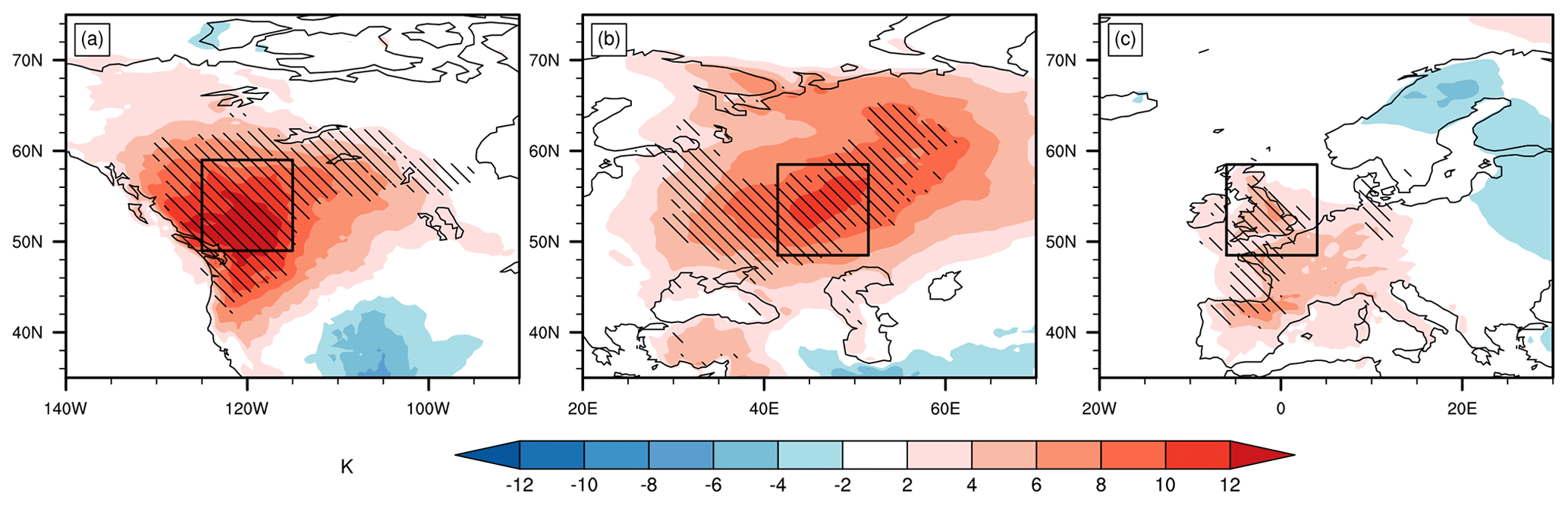
Figure 1Temperature anomalies (5 d averages) on the second-lowest model level during (a) the PNW, (b) the RU, and (c) the UK heatwaves (see Table 1 for the exact periods). Hatching in all panels denotes regions where the previous (since 1979) ERA5 2 m temperature records were broken during the respective 5 d period. The black boxes define the regions we consider here for the three events.
The proximal causes of “benign” heatwaves over mid-latitude land regions are clear and have been elucidated by a plethora of studies: such events typically occur within anticyclonic flows embedded in a slow-moving larger-scale Rossby wave structure, e.g. an atmospheric block (Xoplaki et al., 2003; Meehl and Tebaldi, 2004; Stefanon et al., 2012; Pfahl and Wernli, 2012) or a stationary subtropical ridge (Sousa et al., 2018). The formation of the unusually large positive near-surface temperature anomalies that constitute a heatwave occurs due to three processes: (a) in the upstream part of the anticyclone, air is advected across climatological temperature gradients from climatologically warmer to colder regions. (b) In the central part of the anticyclone, air typically experiences large-scale subsidence, which yields adiabatic warming and leads to clear skies, which (c) enhances the diabatic heating of near-surface air due to strong insolation and resulting sensible heat fluxes (e.g. Fischer et al., 2007; Miralles et al., 2014; Bieli et al., 2015; Zschenderlein et al., 2019; Barriopedro et al., 2023). Moreover, the persistence of the large-scale anticyclonic flow, e.g. due to an upper-level blocking flow or recurrent Rossby wave pattern (Röthlisberger et al., 2019), also increases the persistence of the warm and dry surface conditions (Röthlisberger and Martius, 2019), leaving enough time for soils to dry out and for further amplifying the near-surface heat through land–atmosphere interactions (Fischer et al., 2007; Miralles et al., 2014, 2019).
However, it is far less clear what factors discriminate heatwaves with exceptional magnitudes from less intense events. Case studies focusing on exceptionally intense heatwaves such as the events mentioned above have confirmed the importance of anticyclonic flow patterns, air mass advection, adiabatic warming, clear skies, and dry soils for the existence of these heatwaves (e.g. Dole et al., 2011; Schneidereit et al., 2012; Philip et al., 2022; Faranda et al., 2023), but the causes of their exceptional magnitude remain an area of active research. For the RU and PNW heatwaves, several studies have provided evidence that the atmospheric vertical structure (in particular the vertical temperature structure) during these events was pivotal for determining the magnitude of the near-surface heat. Neal et al. (2022), Schumacher et al. (2022), and Oertel et al. (2023) documented the exceptional mid- to upper-tropospheric warmth during the PNW heatwave, and in particular Neal et al. (2022) and Schumacher et al. (2022) argued that these positive temperature anomalies aloft suppressed convective damping of near-surface temperature anomalies. Along a similar line of reasoning, Zhang and Boos (2023) recently developed a theory for an upper bound of near-surface temperatures during heatwaves over extratropical land, which is based on the assumption that near-surface temperatures are limited by the stability of the atmosphere to moist convection. The authors were able to demonstrate that their theory holds remarkably well for near-surface temperatures and atmospheric profiles from reanalysis data. For the RU heatwave, Miralles et al. (2014) emphasised the importance of the atmospheric vertical structure by revealing that air, diabatically heated during the day and residing in a nocturnal residual layer (far removed from the surface), re-entered the boundary layer on the following day. This diurnal and vertically organised heat accumulation was found to be a pivotal factor in reaching exceptional near-surface temperatures during this event.
In summary, there is accumulating case study evidence (Miralles et al., 2014; Neal et al., 2022; Schumacher et al., 2022) and a theoretical underpinning (Zhang and Boos, 2023) suggesting that the atmospheric vertical structure during heatwaves, in particular the vertical temperature profile, is key for determining the magnitude of exceptionally intense heatwaves. This study now specifically investigates how the vertical temperature structure during the recent record-breaking PNW, RU, and UK heatwaves formed. That is, we quantitatively examine how the interplay between air mass advection across climatological temperature gradients, adiabatic warming and cooling, and diabatic processes shaped the vertical temperature anomaly (T′) profile during these events. As a main analysis tool, we use the Lagrangian T′ decomposition of Röthlisberger and Papritz (2023a), which is based on kinematic backward trajectories and allows for decomposing any T′ of interest into contributions from horizontal air mass advection across climatological T gradients, adiabatic warming and cooling, diabatic processes, and a usually small residual. The Lagrangian T′ decomposition has so far only been applied to near-surface T′ (Röthlisberger and Papritz, 2023a, b). Here, we extend these studies by applying it to the entire tropospheric column above the PNW, RU, and UK heatwaves.
Hereafter, we introduce the data used in this study and then provide a brief introduction to the Lagrangian T′ decomposition (Sect. 2). In Sect. 3, we discuss in detail the characteristics and causes of the atmospheric vertical structure during the PNW heatwave and then contrast it with the atmospheric vertical structure during the Russian and European heatwaves. Finally, we present our conclusions in Sect. 4.
Table 1Definition of the case study regions during the PNW heatwave, the RU heatwave, and the UK heatwave.
2.1 Data
This study uses the European Centre for Medium-Range Weather Forecasts (ECMWF) ERA5 reanalysis (Hersbach et al., 2020) at 3-hourly temporal resolution. Spatially, the data have been interpolated to a resolution of 0.5° latitude by 0.5° longitude and vertically to a stack of pressure levels (from 1000 to 140 hPa in intervals of 20 hPa). Note, however, that for the Lagrangian analyses (see below), we use ERA5 data on the original model levels. The regions of the three heatwaves for which data have been analysed are listed in Table 1. The following ERA5 variables are used: temperature T, potential temperature θ, wind , geopotential height Z, pressure p, sea-level pressure (SLP), potential vorticity (PV), and the height of the planetary boundary layer (PBL). To define the temperature anomalies, T′, we use exactly the same temperature climatology (computed on model levels) as Röthlisberger and Papritz (2023a), which takes into account both the climatological diurnal and climatological seasonal cycles. Specifically, is computed for a given time step by averaging model-level T across all time steps with the same time of the day within 21 d and 9-year windows centred on the time step of interest. That is, each value is the average of 21 × 9 = 189 instantaneous T values. For instance, at 12:00 UTC on 15 July 2010 is computed by averaging model-level T for all 12:00 UTC time steps on all days between (and including) 5 and 25 July, in the years 2006–2014. For the last 5 years of the ERA5 period (extending to December 2022 at the time of analysis), we use the last 9 years of this period to compute . Thus, during the PNW and UK heatwaves is computed based on data from the years 2014–2022. Wherever daily averages are presented, they refer to averages over UTC (and not local) days, i.e. comprising eight time steps from 00:00 to 21:00 UTC.
2.2 Stability to moist convection
Zhang and Boos (2023) convincingly argued that the largest possible magnitude of a heatwave is limited by the stability of the atmosphere to moist convection. That is, near-surface temperatures can only rise until the atmospheric profile becomes unstable to moist convection, which would cool the surface through reduced insolation and precipitation. This argument provides a key motivation for studying the atmospheric vertical structure during heatwaves, in particular in cases where there is indeed a convective coupling between near-surface and free tropospheric levels, i.e. in cases when the atmospheric vertical structure is near neutral to moist convection. Here, we quantify the stability of the atmosphere to moist convection during our three events of interest by exactly following the reasoning put forward in Zhang and Boos (2023). Specifically, we compute and compare the moist static energy at the surface (MSEs) and the saturation moist static energy at 500 hPa () as
and
respectively, whereby cp denotes the specific heat of air at constant pressure; Ts and T500 are the 2 m and 500 hPa temperatures, respectively; Lv is the latent heat of vaporisation; qs is the 2 m specific humidity; qsat(T500) is the saturation specific humidity at T500; g is the gravitational acceleration; and zs and z500 are the height of the surface and the 500 hPa pressure level, respectively. Note that we approximate , whereby ϵ is the molar ratio between water vapour and dry air, and es(T500) is the saturation vapour pressure at T500 derived from the Clausius–Clapeyron relation.
As in Zhang and Boos (2023), a moist convectively unstable stratification is identified when . We examined at individual grid points as well as in a spatially aggregated manner and chose to present spatially aggregated below.
2.3 Computation of backward trajectories
The computation of backward trajectories in this study is exactly analogous to the approach of Röthlisberger and Papritz (2023a). We use the Lagrangian analysis tool LAGRANTO 2.0 (Sprenger and Wernli, 2015) to compute 15 d backward trajectories, started at each 3-hourly time step from each heatwave region (see Table 1 and text below) and at various vertical levels. Trajectory information is stored at a 3-hourly temporal resolution as well. For the analysis of near-surface T′, trajectories are started at 10, 30, and 50 hPa above ground level. Hereby, we start trajectories from multiple near-surface levels to improve the robustness of our results (e.g. Bieli et al., 2015), as some boundary layer processes such as turbulent mixing cannot be expected to be fully resolved at 0.5° horizontal resolution. Furthermore, for the analysis of the vertical T′ structure, additional trajectories are started between 1000 and 175 hPa in 25 hPa steps above each heatwave region. No trajectories were started at grid points and levels where the respective level intersected or was located below the local topography. Along each trajectory (x(t),t), where x(t) = at each trajectory time step t, the following variables are traced: T, , θ, , and . Thereby, the quantities and are computed using first-order finite differences.
2.4 Lagrangian T′ decomposition
The Lagrangian T′ decomposition of Röthlisberger and Papritz (2023a) builds conceptually on several previous studies that evaluated the thermodynamic energy equation along kinematic backward trajectories to investigate how adiabatic warming and diabatic heating affected the temperature in the air that subsequently contributed to near-surface temperature extremes (e.g. Bieli et al., 2015; Santos et al., 2015; Quinting and Reeder, 2017; Zschenderlein et al., 2019; Papritz, 2020). The novel aspect of the Röthlisberger and Papritz (2023a) approach is that it considers the material change of T′ instead of T and thereby also allows for quantifying the effect of air parcel advection across horizontal gradients of on T′. The decomposition of any , where tf refers to the starting time of the trajectory, is obtained by re-writing the thermodynamic energy equation in terms of T′ and then integrating it along a backward trajectory started at (x,tf) from the time when T′ was last 0 in the respective air parcel (hereafter referred to as “genesis time”, tg) to tf, i.e.
Hereby, v is the horizontal wind, ∇h the horizontal gradient operator, and (see Röthlisberger and Papritz (2023a) for a formal derivation of Eq. 3). As in Röthlisberger and Papritz (2023a), the terms on the right-hand side of Eq. (3) are hereafter referred to as seasonality T′, advective T′, adiabatic T′, and diabatic T′. For the details of computing the individual terms in Eq. (3), the interested reader is referred to Röthlisberger and Papritz (2023a). Moreover, when evaluating Eq. (3) for discrete trajectory data, a first residual appears because T′ is never exactly 0, and thus 1. A second residual appears due to inaccuracies in the computation of derivatives in Eq. (3). As in Röthlisberger and Papritz (2023a), we compute an overall residual in order to assess how well the T′ budget closes by just considering advective T′, adiabatic T′, and diabatic T′. We find that res is typically small compared to these three terms (for detailed information, see Röthlisberger and Papritz, 2023a).
Furthermore, knowledge of the genesis time tg for any temperature anomaly (i.e. the time when the respective air parcel last had 0 T′) allows for computing the Lagrangian age of as the difference between tf and tg. Similarly, the spatial scale, over which formed, can be quantified by computing the Lagrangian formation distance as the great circle distance between x(tg) and x(tf).
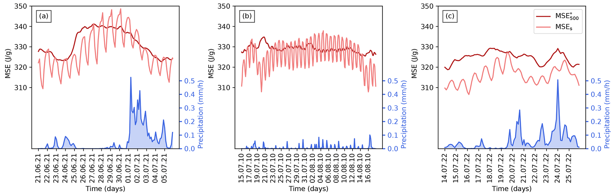
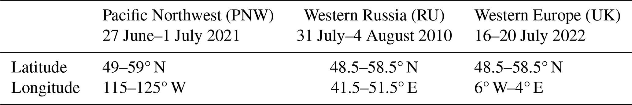
Figure 2Surface moist static energy (MSEs; light red) and free tropospheric saturation moist static energy (; dark red) evolution during the (a) PNW heatwave, (b) RU heatwave, and (c) UK heatwave. The blue line and shading depict precipitation (right y axis). All values have been averaged over the respective 10.5° latitude by 10.5° longitude boxes indicated in Fig. 1.
2.5 Event definition
To define the temporal and spatial extent of the PNW, RU, and UK heatwaves, we applied the following procedure: first, we identify the grid point with the largest positive daily mean near-surface (second-lowest model level) temperature anomaly in the respective region and year with existing literature on heatwaves serving as a first approximation for the heatwave regions and periods (these dates and locations are hereafter referred to as peak locations and peak times). Then, we define for each event the temporal extent as the 5 d period centred on the respective peak day and the spatial extent as the 10.5° latitude by 10.5° longitude box centred on the respective peak location. This approach yields the heatwave periods and regions indicated in Table 1 and Fig. 1.
For the PNW and RU heatwaves, the selected regions and periods correspond well with event definitions used in previous studies (e.g. Dole et al., 2011; Hauser et al., 2016; Philip et al., 2022; Neal et al., 2022; Schumacher et al., 2022; Röthlisberger and Papritz, 2023a), while for the very recent UK heatwave (with few studies detailing this event so far), our selected period also contains 19 July 2022, when temperatures exceeding 40 °C were first measured in the UK (Yule et al., 2023). Moreover, during the so-defined heatwave periods, ERA5 surface temperature records were broken across the heatwave regions in all three cases (Fig. 1).
We have extensively tested the sensitivity of our results to shifts in the spatial extent, location, and timing of the heatwave regions and periods. Qualitatively, our results are insensitive to horizontal shifts in the heatwave regions by a few degrees latitude and/or longitude, enlarging or shrinking the regions by a few degrees in either direction, and shifts in the heatwave periods by 1–2 d, as long as the main synoptic events of interest are still contained within the heatwave regions and periods (not shown). Note, however, that the RU heatwave lasted for over a month (Barriopedro et al., 2011). Here, we focused on its peak phase; thus we cannot exclude the possibility that our results may be sensitive to much larger shifts in the respective heatwave period.
3.1 Stratification during the PNW, RU, and UK heatwaves
We begin by examining the stratification during the PNW, RU, and UK heatwaves (Fig. 2). Figure 2 shows time series of and MSEs, alongside with precipitation, each spatially averaged over the respective heatwave region. A positive sign of indicates a stratification that is stable to moist convection (i.e. no convective coupling), a negative sign indicates a moist convectively unstable stratification, and a value of 0 implies moist convective neutrality (e.g. Zhang and Boos, 2023). A heatwave during which convective instability plays no role in limiting near-surface temperatures would thus feature positive values of throughout the entire event, in which case the arguments by Zhang and Boos (2023) would not be expected to hold.
In particular for the PNW heatwave, Fig. 2 supports the notion of a top-down control of near-surface temperatures via convective instability. Firstly, peaked before MSEs, which indicates that mid-tropospheric temperatures already rose before the near-surface temperatures soared to record highs. Secondly, time series of and MSEs suggest a moist convectively unstable stratification during the peak of the heatwave, while the termination of the heatwave coincided with a large precipitation peak. Hereby, negative values of (indicating unstable conditions) during the heatwave peak (i.e. before precipitation occurred) might have been sustained over multiple hours by entrainment of dry air into air parcels ascending through the PBL (as suggested by Zhang and Boos, 2023) or by considerable convective inhibition (CIN) related to a strong boundary layer inversion (Neal et al., 2022; Fig. S1a in the Supplement).
During the UK heatwave, peaked on 18 July 2022, while MSEs peaked on 19 July, when it just reached the respective value of . Convective coupling between mid-tropospheric and near-surface air is thus less evident for the UK heatwave than for the PNW heatwave, but as for the PNW heatwave, its termination (20 July 2022) did co-occur with a peak in precipitation (Fig. 2c).
During the RU heatwave, the daily maximum of MSEs regularly exceeded during the afternoon time steps, in particular also during its peak time (31 July to 4 August 2010), indicating convective coupling of near-surface and mid-tropospheric air during more than 2 weeks (Fig. 2b). Small amounts of diurnal precipitation occurred throughout the event but evidently did not terminate the RU heatwave. Thus, while convective instability may have limited the near-surface temperatures during the RU heatwave to some degree, Fig. 2b suggests that for the termination of a heatwave, diurnal moist convection may not always suffice, in particular when moisture is strongly limited and soils have already dried out considerably, as was the case during the RU heatwave (Lau and Kim, 2012; Wehrli et al., 2019).
In summary, Fig. 2 suggests that in particular during the PNW and RU heatwaves, and to some degree also during the UK heatwave, near-surface air was convectively coupled to mid-tropospheric air during their peak phases. This implies that convective instability, and with it the vertical temperature structure, likely played an important role in limiting the magnitude of at least the PNW and RU heatwaves, while its role in the UK heatwave is more ambiguous. In the next sections we thus provide a detailed analysis of the characteristics and synoptic causes of the vertical temperature structure during these three events. Specifically, we first discuss in detail the vertical temperature structure of the PNW heatwave and then compare and contrast it with that of the RU and UK heatwaves.
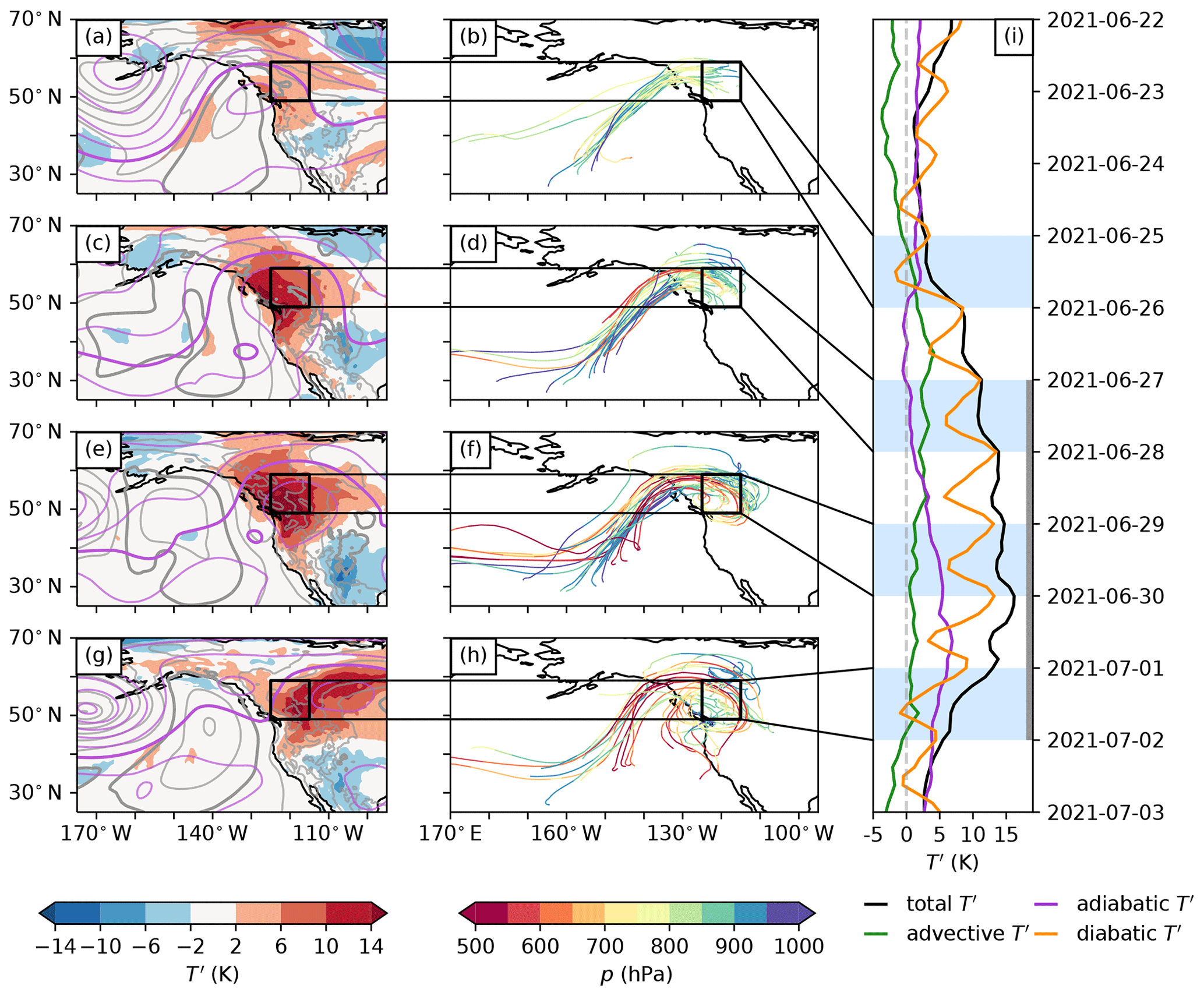
Figure 3The synoptic evolution of the PNW heatwave daily averaged on (a, b) 25 June 2021, (c, d) 27 June 2021, (e, f) 29 June 2021, and (g, h) 1 July 2021 and (i) the near-surface T′ and its contribution between 22 June and 3 July 2021. The left panels (a, c, e, and g) show the T′ at the second-lowest model level in colour, the mean SLP (in 5 hPa steps, with the 1020 hPa contour highlighted in bold) in grey contours, the geopotential height at 500 hPa (in 100 m steps, with the 5800 m contour highlighted in bold) in purple contours, and the PNW heatwave region as a black rectangle. The middle panels (b, d, f, and h) show 30 selected trajectories with positive T′ (coloured according to their pressure) arriving near the surface (10 trajectories each arriving at 10, 30, and 50 hPa above ground level) on land grid points in the case study region at each date. Trajectories are only shown for trajectory time t for which t≥tg. The right panel (i) shows the near-surface T′ (black), advective T′ (green), adiabatic T′ (purple), and diabatic T′ (orange) averaged over land grid points of the PNW heatwave region from 24 June to 3 July 2021. The grey line denotes the PNW heatwave period.
3.2 The PNW heatwave
3.2.1 Synoptic situation and evolution of near-surface T′
The synoptic evolution of the PNW heatwave has already been extensively examined in previous studies (e.g. Philip et al., 2022; Schumacher et al., 2022; Neal et al., 2022; White et al., 2023; Röthlisberger and Papritz, 2023a) and is thus only revisited here to a minimal extent to provide a synoptic context for the subsequent findings. A key synoptic ingredient in this event was an upstream cyclone (visible in the top left of Fig. 3a) which deepened rapidly between 22 and 25 June. This cyclone produced a warm conveyor belt (WCB), which built up the extremely amplified (e.g. in terms of potential temperature on the dynamical tropopause; Oertel et al., 2023) upper-tropospheric quasi-stationary ridge, within which the heatwave occurred on the subsequent days.
In the early stage of the heatwave, between 25 and 26 June, near-surface T′ in the PNW heatwave region built up diabatically as well as advectively (Fig. 3i) and formed in air parcels that moved into the amplifying ridge and subsequently onshore (Fig. 3b). Since their respective tg, most of these air parcels first ascended over the Pacific (whilst moving poleward into the ridge) and subsequently descended before they contributed to the positive near-surface T′ between 25 and 26 June (shown for selected trajectories in Fig. 3b and d).
Between 27 June and the peak of the heatwave on 30 June, the ridge axis was located above the PNW heatwave region, where the average near-surface T′ exceeded +10 K (Fig. 3c and e). The better part of the T′ formed diabatically, but there was a gradual increase in the adiabatic contribution to near-surface T′ throughout the heatwave (Fig. 3i). This increase in the adiabatic T′ was also associated with a change in the behaviour of the trajectories of near-surface air, which increasingly started to spiral downward and anticyclonically near the PNW heatwave region (compare Fig. 3d and f).
After the peak of the heatwave (with spatially averaged near-surface temperature anomalies of roughly +15 K), on 30 June and 1 July, the total T′ and the diabatic T′ dropped significantly, consistent with the convective termination of the event and the associated onset of precipitation (see Fig. 2a). Note that even though the ridge started shifting eastward between 30 June and 1 July, it was only on 2 July that the advective T′ became negative and thus indicates the advection of air from climatologically colder regions into the heatwave region (Fig. 3i). This is consistent with the termination of the PNW heatwave being due to convective damping of near-surface T′ rather than due to changes in air mass advection into the region.
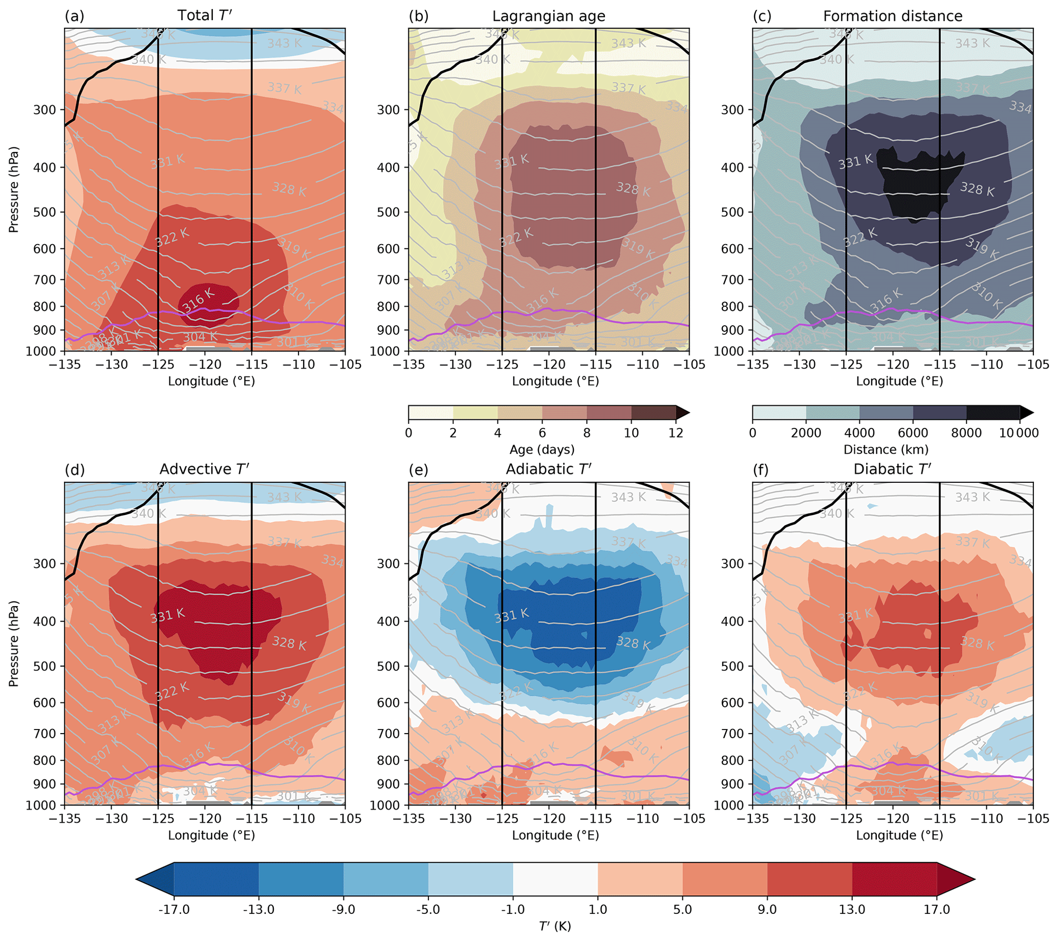
Figure 4The 5 d mean (27 June–1 July 2021) vertical cross-section showing the T′ decomposition during the PNW heatwave. Fields are latitudinally averaged between 49–59° N over land grid points. The panels show (a) T′, (b) the Lagrangian age, (c) the formation distance, (d) the advective T′, (e) the adiabatic T′, and (f) the diabatic T′ in colour. The black line depicts the dynamical tropopause (2 PVU contour; 1 PVU=106 ), grey contours show potential temperature, and the purple line shows the PBL height. In addition, the grey colour shows altitudes without grid points above the topography. The two vertical black lines indicate the longitudinal extent of the PNW heatwave region.
3.2.2 Time-mean vertical structure of T′
We first discuss time-mean characteristics of the vertical T′ structure of the PNW heatwave (Fig. 4). Previous studies have already identified anomalous warmth throughout the troposphere during the PNW heatwave (Neal et al., 2022; Schumacher et al., 2022; Oertel et al., 2023; Zhang and Boos, 2023). Consistent with these results, we find positive 5 d average T′ in excess of +5 K throughout the troposphere, reaching up to 300 hPa (Fig. 4a). Applying the Lagrangian T′ decomposition to the entire volume of air above the PNW heatwave, from the surface to 200 hPa, allows for quantitatively examining the physical causes and vertical structure of these deep positive T′ values (Fig. 4d–f). For T′ between 300 and 600 hPa, we find large positive contributions from advective T′ (exceeding +13 K) and diabatic T′ (roughly +9 to +13 K), as well as pronounced negative contributions from adiabatic T′ (less than −13 K, Fig. 4d–f). That is, after the respective anomaly genesis, these air parcels ascended in a poleward motion and thereby experienced considerable diabatic heating (presumably due to cloud formation), which is exactly the signature expected from a WCB. These results thus quantitatively substantiate the results of Neal et al. (2022), Schumacher et al. (2022), and Oertel et al. (2023), who qualitatively argued that this positive temperature anomaly originated from the WCB.
The 5 d mean T′ peaked between 700 and 850 hPa with values larger than +13 K. In contrast to the air further aloft, these anomalies featured positive contributions from all three processes with roughly equal magnitude. That is, this air also moved from climatologically warmer regions towards the PNW heatwave region and experienced net diabatic heating since the respective tg (albeit to a lesser extent than the air further aloft). However, contrary to the mid- to upper-tropospheric air, these air parcels experienced net subsidence since tg, which manifested itself as positive adiabatic T′. This strong vertically aligned dipole, with positive and negative adiabatic T′ within an anticyclone, is perhaps surprising at first sight, as it is frequently argued that within anticyclones the subsidence contributes significantly to positive temperature anomalies in anticyclones (Pfahl and Wernli, 2012; Bieli et al., 2015; Zschenderlein et al., 2019). A close inspection of the trajectories' pressure evolution reveals that, indeed, throughout the column above the PNW heatwave, the air subsided in the anticyclone (yielding a positive adiabatic T′ for the part of the trajectory since the lowest pressure was reached, Fig. S2). However, what matters for the net effect of vertical motion on T′ (i.e. the total adiabatic T′) is the net vertical motion since the time when the air parcel last had 0 T′, i.e. since tg. For the PNW heatwave, we find that air parcels ending up in the heatwave region on levels above 600 hPa first experienced a strong and fast ascent within the WCB, which covered a larger pressure difference than the subsequent slow descent within the anticyclone, yielding a net negative adiabatic T′. Conversely, for air parcels below 600 hPa, the subsidence within the anticyclone was larger than the ascent experienced on the way into the anticyclone, yielding positive adiabatic T′ at lower levels.
In the PBL, the contributions from adiabatic and, in particular, diabatic T′ jointly account for the bulk of the total T′. Hereby, this lower-tropospheric diabatic T′ maximum is conceivably related to sensible and turbulent heat fluxes from the surface to the atmosphere, contrary to the upper-tropospheric diabatic T′ maximum, which is likely due to upstream cloud diabatic heating. Note that the large diabatic contribution to near-surface T′ found here is also in agreement with previous studies, which used an array of different methods to arrive at the same conclusion (Schumacher et al., 2022; Neal et al., 2022; Conrick and Mass, 2023).
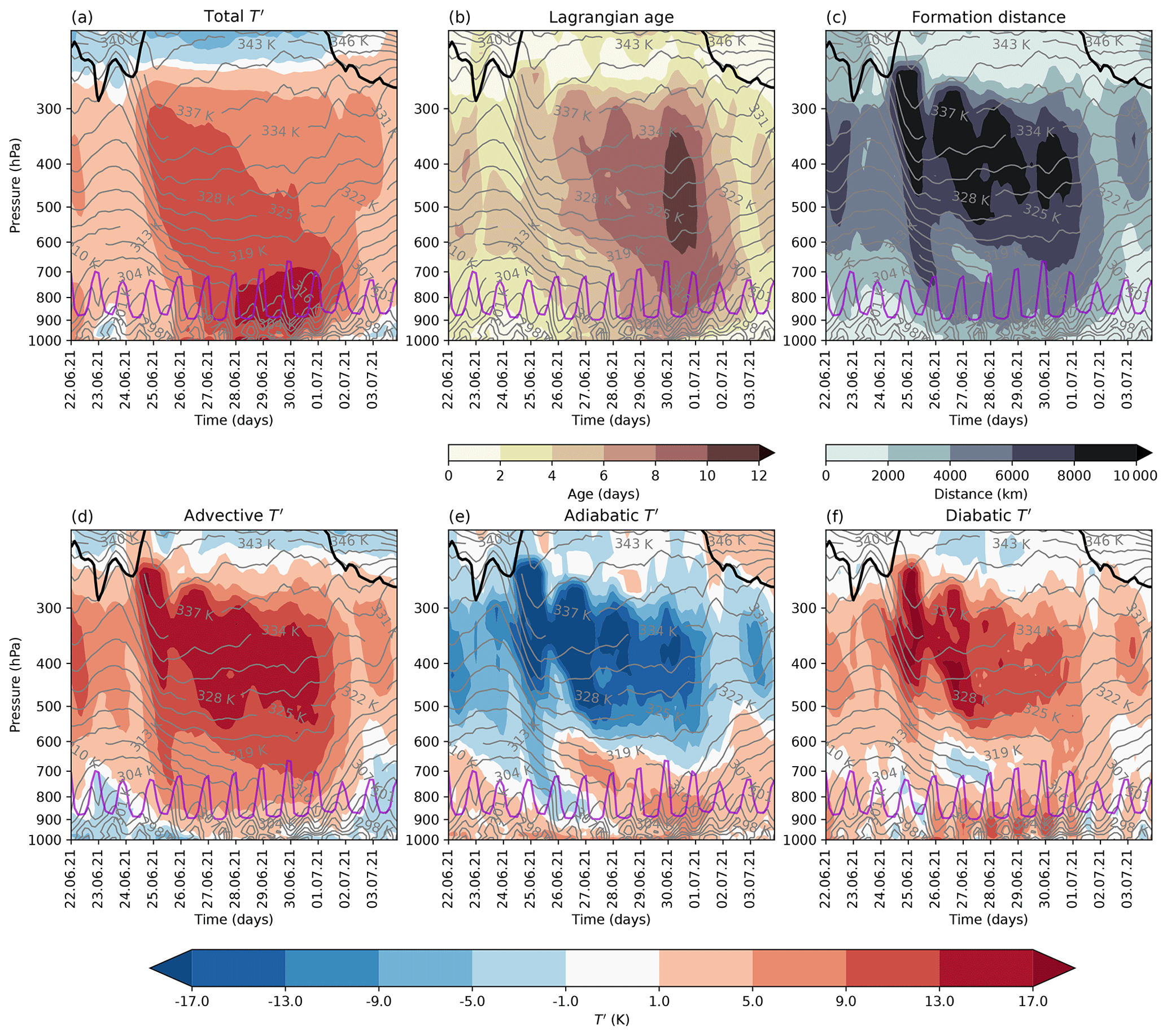
Figure 5Time–height plots showing the T′ decomposition during the PNW heatwave spatially averaged over land grid points in the PNW heatwave region between 22 June and 3 July 2021. The panels show (a) T′, (b) the Lagrangian age, (c) the formation distance, (d) the advective T′, (e) the adiabatic T′, and (f) the diabatic T′ in colour. The black line shows the dynamical tropopause (2 PVU contour), the grey contours depict the potential temperature, and the purple line indicates the PBL height.
By determining the Lagrangian age and formation distances (Fig. 4b and c), the temporal and spatial scales over which the temperature anomalies form can be quantified. For the mid- to upper-tropospheric air over the PNW heatwave region, we find ages of 8–10 d (Fig. 4b) and formation distances (Fig. 4c) of several thousand kilometres (at some levels exceeding 8000 km). These age values and formation distances are 2 to 3 times larger than those of near-surface T′.
3.2.3 Evolution of the vertical T′ structure
Next, we examine the specifics of the temporal evolution of the vertical T′ structure (Fig. 5). A first point to notice is that large positive T′ first emerged at upper levels and only several days later appeared near the surface. In accordance with Schumacher et al. (2022) and Zhang and Boos (2023), we find a first pulse of T′ formation at mid- to upper-tropospheric levels (exceeding 9 K) on 24 and 25 June, while in the PBL, T′ ranged between −5 and +5 K (Fig. 5a). Positive advective and diabatic T′ and negative adiabatic T′ now quantitatively underline that this warming aloft was due to the aforementioned WCB, as qualitatively demonstrated by Neal et al. (2022), Zhang and Boos (2023), and Schumacher et al. (2022). This WCB signature between roughly 600 and 300 hPa persisted throughout the heatwave until 1 July and was associated with particularly large formation distances (Fig. 5c).
Second, Fig. 5f shows evidence of diurnal heat accumulation in the PBL, as observed in earlier mega heatwaves by Miralles et al. (2014). The positive diabatic T′ in the PBL increased from 26 to 30 June. While there was a diurnal cycle in the generation and decay of diabatic T′, not all of the positive diabatic T′ decayed during the night, and some of it persisted until the next morning, in particular in the residual layer above the PBL. On the following day, when the PBL grew again in depth, the air from the residual layer was likely again mixed into the PBL. Albeit not definitive proof, these observations support the hypothesis of multi-day heat accumulation in the PBL in the sense of Miralles et al. (2014).
Third, there is evidence of downward propagation of positive adiabatic T′ in the lower troposphere (Fig. 5e). Interestingly, the peak in near-surface T′ (around 30 June 2021) coincided with the time when the adiabatic T′ peaked in the PBL. This is consistent with the hypothesis that during the peak days of the PNW heatwave, some of the air that was mixed into the PBL during the diurnal PBL growth had been significantly heated adiabatically before (Schumacher et al., 2022), although note that a vertical propagation of signals in Fig. 5 over time does not necessarily imply that the same air parcels contribute to that signal at different time steps.
Fourth, the age of mid- to upper-tropospheric T′ and PBL T′ increased considerably over the course of the PNW heatwave (Fig. 5b). On 25 June, the age of T′ at 400 hPa was 4–6 and 2–4 d at 900 hPa. By 30 June, Lagrangian ages of 400 hPa T′ reached 10–12 d, whilst at 900 hPa T′ was 6–8 d old. Therefore, ageing of T′ is observable throughout the tropospheric column above the PNW heatwave.
In summary, the temporal evolution of the vertical T′ structure and the time series of precipitation, , and MSEs support the notion of a top-down control on near-surface T′ via convective (in)stability and provide qualitative evidence of multi-day diurnal heat accumulation in the PBL preceding the peak of the heatwave (as described in Miralles et al., 2014), which also coincided with the time when strongly adiabatically warmed air was mixed into the PBL (Schumacher et al., 2022). Furthermore, Fig. 5b, for the first time, documents the ageing of T′ throughout the PNW heatwave, which has been qualitatively surmised by previous studies putting forward the concept of a heat dome (Neal et al., 2022; Zhang et al., 2023). In the next sections, we contrast the characteristics and evolution of the vertical T′ structure during the PNW heatwave with that of the RU and UK heatwaves.
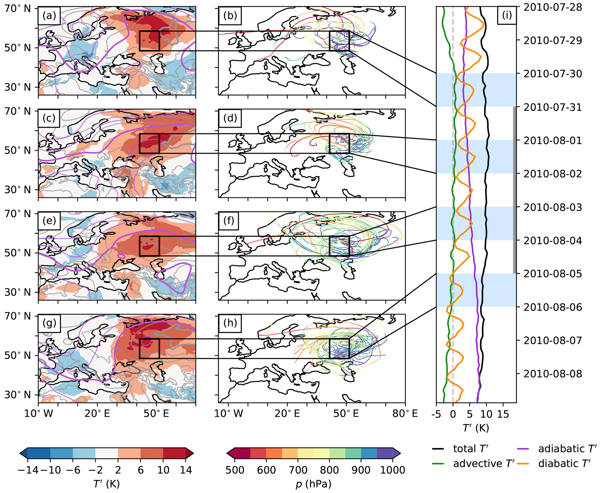
Figure 6As Fig. 3 but for the RU heatwave. Panels are shown for (a, b) 1 August 2010, (c, d) 3 August 2010, (e, f) 5 August 2010, (g, h) 7 August 2010, and (i) 28 July–8 August 2010.
3.3 Comparing the PNW, RU, and UK heatwaves with regard to their vertical T′ structure
3.3.1 Comparing and contrasting the RU and PNW heatwaves
Another record-shattering and intensely studied heatwave occurred in western Russia in 2010, lasting from mid-July to mid-August (Barriopedro et al., 2011; Dole et al., 2011; Lau and Kim, 2012). This heatwave was associated with an exceptionally long-lasting and stationary anticyclone (Barriopedro et al., 2011; first column of Fig. 6), which was embedded within a larger-scale Rossby wave train (Lau and Kim, 2012; Trenberth and Fasullo, 2012; Schneidereit et al., 2012). Here, we briefly describe the formation of near-surface T′ and the vertical T′ structure during the peak time of the RU heatwave and then contrast these results to those discussed before for the PNW heatwave.
The trajectories of air parcels contributing to the RU heatwave at near-surface levels between 31 July and 4 August 2010 subsided in an anticyclonically spiralling motion prior to reaching near-surface levels (Fig. 6b, d, f, and h). During the 5 d maximum T′ (grey-coloured bar in Fig. 6i), the diabatic T′ exhibited a pronounced diurnal cycle and, in terms of daily means, decreased slightly, from +7 K to +5 K, while the adiabatic T′ increased from +3 to +7 K. At the same time, the advective T′ remained near 0. Throughout the 5 d period, the adiabatic and diabatic contributions were of comparable magnitude. While these results are consistent with those of Zschenderlein et al. (2019), they are in some contrast to other studies that emphasised, in particular, the importance of diabatic processes due to prolonged soil moisture depletion (e.g. Trenberth and Fasullo, 2012; Barriopedro et al., 2011; Miralles et al., 2014; Hauser et al., 2016). This is particularly noteworthy, as, in both absolute and relative terms, the RU heatwave featured far smaller diabatic contributions to its near-surface T′ than the PNW heatwave (compare Figs. 6i and 3i). Moreover, the adiabatic contribution grew steadily throughout the evolution of the heatwave and eventually clearly exceeded the diabatic contribution.
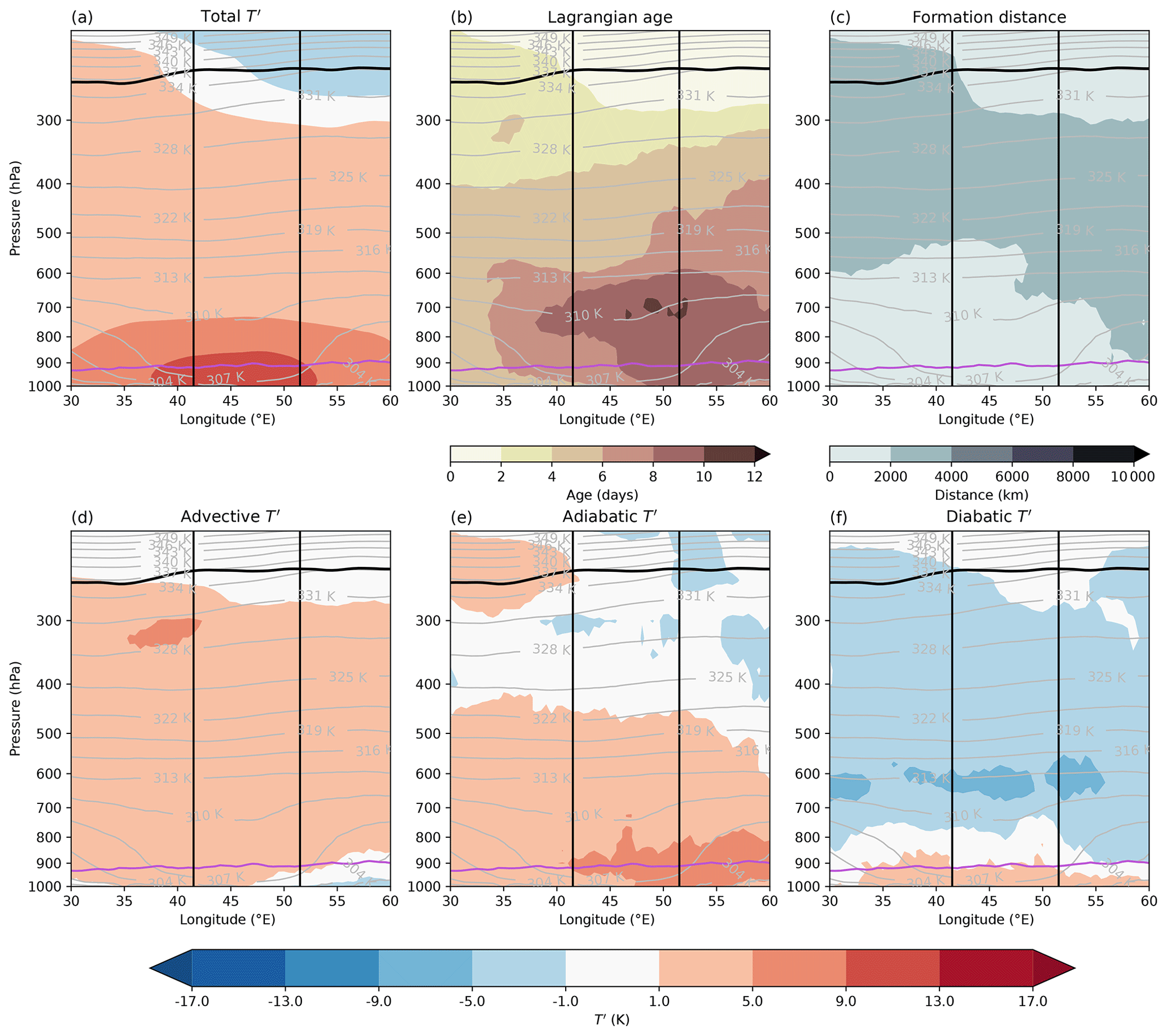
Figure 7As Fig. 4 but for the RU heatwave. Latitudinal averages are taken over 48.5–58.5° N over the period from 31 July to 4 August 2010.
The vertical T′ structure of the RU heatwave featured a number of similarities to that of the PNW heatwave (compare Figs. 7 and 4). For instance, during both heatwaves, the positive T′ extended throughout the troposphere (see also Fig. S2 in Zhang and Boos, 2023). Moreover, during both heatwaves mid- to upper-tropospheric T′ featured large positive advective contributions (Figs. 4d and 7d), while large positive adiabatic T′ was restricted to the lower troposphere. Furthermore, a clear maximum in diabatic T′ occurred near the surface (Fig. 7f).
However, clear differences that point to differing synoptic dynamics involved in the two events also emerge: the prominent WCB signature aloft (positive advective and diabatic T′, negative adiabatic T′) during the PNW heatwave was not apparent during the RU heatwave. Rather, the diabatic T′ in the upper troposphere during the RU heatwave was negative, presumably due to radiative cooling. These results suggest that the anticyclone associated with the RU heatwave was not as strongly diabatically driven as the one during the PNW heatwave. Moreover, we find almost isobaric flow in the upper troposphere during the RU heatwave (not shown), which is consistent with barotropic Rossby wave dynamics as the main driver of this anticyclone.
The two heatwaves also differed considerably regarding the Lagrangian age and formation distances of their T′. During the PNW heatwave, the oldest anomalies (> 8 d) were located between 600 and 300 hPa, whereby those anomalies featured the WCB signature. During the RU heatwave, the oldest T′ (> 10 d) was located below 600 hPa and, in contrast to the oldest anomalies during the PNW heatwave, featured comparatively small formation distances of less than 2000 km (Fig. 4c). That is, in contrast to the oldest anomalies in the PNW heatwave, these oldest anomalies of the RU heatwave built up more locally, whilst recirculating and subsiding in the anticyclone. In summary, these contrasts regarding the WCB signature in the T′ composition of mid- to upper-level T′ during the PNW and RU heatwaves show that an upstream WCB may amplify an anticyclone within which subsequently a major heatwave occurs (e.g. during the PNW heatwave), but this is clearly not a necessary condition for a major heatwave to occur (e.g. the RU heatwave).
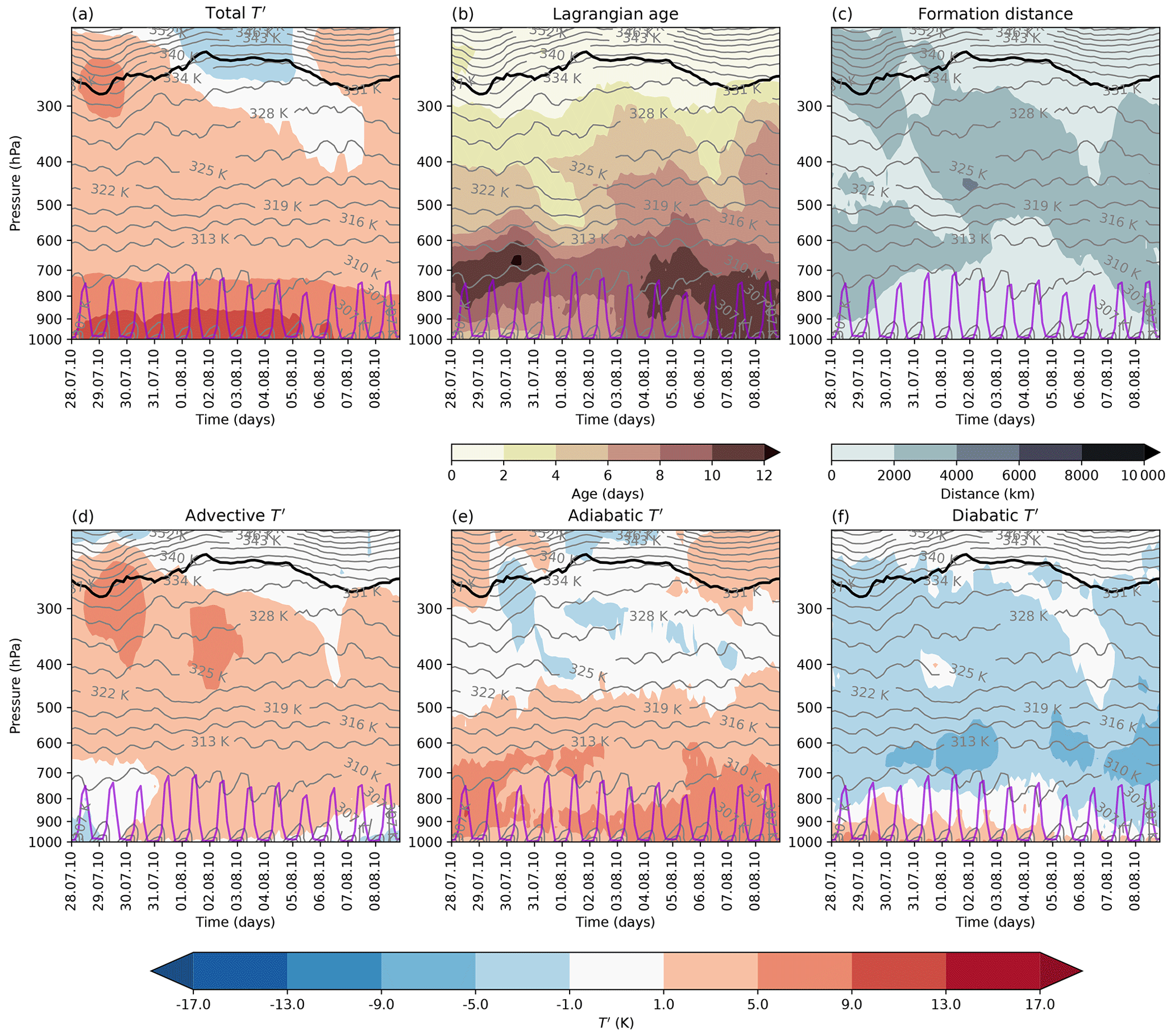
Figure 8As Fig. 5 but for the RU heatwave between 28 July and 8 August 2010. Spatial averages are taken over land grid points in the RU heatwave region.
Next, we contrast the evolution of the vertical T′ structure during the RU and PNW heatwaves (compare Figs. 5 and 8). During the RU heatwave, positive T′ extended throughout almost the entire troposphere with far less temporal variation than during the PNW heatwave, which is unsurprising given that the RU heatwave lasted for over a month (Barriopedro et al., 2011; Dole et al., 2011; Lau and Kim, 2012; Zhang and Boos, 2023). Hereafter, we focus on the selected peak period from 31 July to 4 August 2010.
By and large, the advective, adiabatic, and diabatic T′ featured only small temporal variations in contrast to the PNW heatwave, particularly in the free troposphere, where the Lagrangian formation distance also only changed marginally during that period (Fig. 8c–f). In the free troposphere, advective T′ was positive above 500 hPa, with small values below; adiabatic T′ was positive below 500 hPa, with small values above; and diabatic T′ was consistently negative throughout the entire free troposphere. The unusual persistence of the RU heatwave was thus also reflected in a rather stationary and persistent vertical T′ structure.
However, similarly to the PNW heatwave, the PBL height during the RU heatwave featured a pronounced diurnal cycle and regularly reached nearly 700 hPa during the afternoon. As also documented by Miralles et al. (2014), evidence of diurnal heat accumulation (i.e. positive diabatic T′ persisting overnight in a residual layer above the PBL) is apparent predominantly between 28 and 31 July 2010, i.e. when near-surface T′ was still accumulating. Later during the heatwave (in early August), large positive adiabatic T′ but small diabatic T′ above the nighttime PBL suggests that the maintenance of extremely large PBL T′ was aided by the mixing of adiabatically heated air into the diurnally growing PBL. However, a key difference between the PNW and RU heatwaves in the PBL concerns the depth of the vertical layer with positive diabatic T′ near the surface, which was far shallower during the RU compared to the PNW heatwave. It is currently unclear how exactly this result is to be interpreted.
Surprisingly, the diabatic T′ declined within the lowermost 200 hPa from 29 July onwards, while the adiabatic contributions grew steadily. This contrasts the findings of Miralles et al. (2014) and Zschenderlein et al. (2019), who emphasised the importance of sensible heat fluxes during the RU heatwave, and also distinguishes it from the PNW heatwave.
Finally, similarly to the PNW heatwave also during the RU heatwave, T′ values in the lower troposphere were ageing (Fig. 8b) during the peak phase of this event. For instance, at 950 hPa, the age of T′ increased from 4–6 d on 30 July to more than 10 d on 8 August.
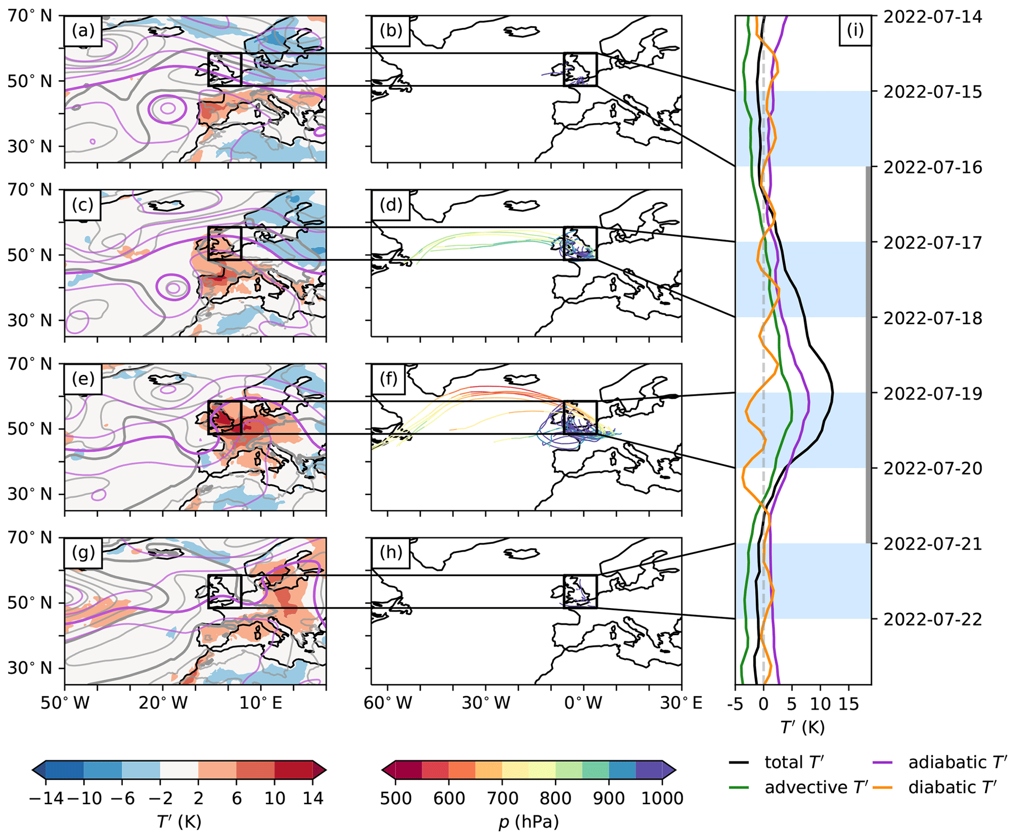
Figure 9As Fig. 3 but for the UK heatwave. Panels shown for (a, b) 15 July 2022, (c, d) 17 July 2022, (e, f) 19 July 2022, (g, h) 21 July 2022, and (i) 14 July–22 July 2022. The positive T′ trajectories in panels (b, h) are particularly short since positive T′ values are only a few hours old.
3.3.2 Contrasting the UK heatwave to the RU and PNW heatwaves
As a third case study, we examine the western European and UK heatwave in July 2022, during which at 46 stations in the UK, the previous nationwide temperature record of 38.7° C was broken (Press Office, 2022). Before the heatwave hit the case study region, positive near-surface T′ formed over the Iberian Peninsula under a subtropical ridge (Fig. 9a) and downstream of a cutoff cyclone located in the eastern North Atlantic. The ridge then further extended to the north and moved eastwards (Fig. 9c, e, and g) towards the UK and western Europe. Throughout the event, large positive near-surface T′ values were first found in the Iberian Peninsula and then over the British Isles, followed by Germany (Fig. 9).
During the 5 d T′ maximum in our selected heatwave region, the adiabatic T′ contribution was dominant (Fig. 9i), which agrees with the findings of Bieli et al. (2015) and Zschenderlein et al. (2019), who climatologically studied air mass origins during heatwaves over the British Isles and emphasised the importance of subsidence for these events. However, the advective T′ contribution, exceeding +4 K on 19 July, was also substantial. Furthermore, in stark contrast to the other two events, the diabatic T′ is near 0 or even negative (Fig. 9i). One of the reasons for this discrepancy might be that during the UK heatwave, near-surface air parcels approached the UK from the North Atlantic and on near-surface levels (Fig. 9b, d, f, and h), where anomalously warm air is typically cooled through sensible heat fluxes (Röthlisberger and Papritz, 2023a). Finally, note that the UK heatwave lasted considerably shorter than the other two heatwaves and ended swiftly after the 5 d T′ maximum.
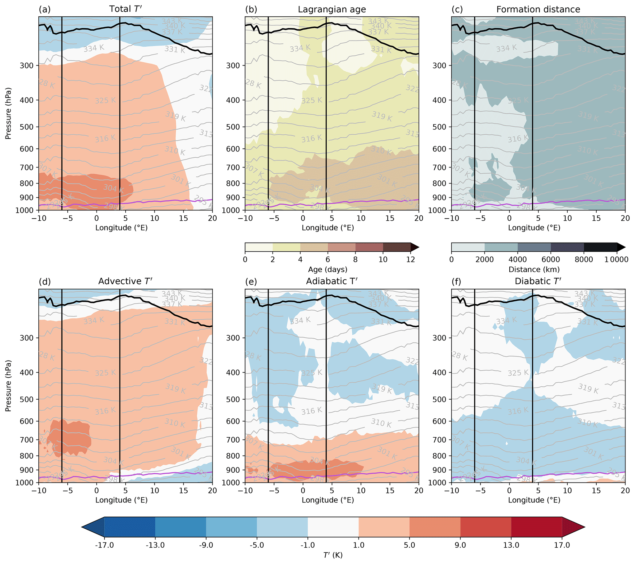
Figure 10As Fig. 4 but for the UK heatwave. Latitudinal averages are taken over 48.5–58.5° N over the peak period from 16 to 20 July 2022.
Next, we examine the time-mean vertical T′ structure during the UK heatwave (Fig. 10). In the 5 d mean, positive T′ extended throughout the troposphere, similarly to the PNW and RU heatwaves (Fig. 10a). The maximum T′ was located around 875 hPa. Above the PBL, the UK heatwave featured a qualitatively similar vertical T′ structure to the RU heatwave, with a layer of positive adiabatic T′ extending from the surface to roughly 700 hPa (500 hPa during the RU heatwave, Figs. 7e and 10e; note that such a layer with positive adiabatic T′ was also apparent during the PNW heatwave, Fig. 4e) and above that positive T′ consisting of positive advective T′ and modest negative contributions from adiabatic and diabatic T′.
A clear contrast between the UK heatwave and the other two events is that the diabatic T′ was negative in the heatwave region, even near the surface, and ranged between near 0 and −5 K in the free troposphere (Fig. 10f). Thereby, the near-surface diabatic T′ increased towards the east, i.e. over European land regions (Fig. 10e). Furthermore, the age of T′ during the UK heatwave was considerably smaller than during the two other events, in particular for the largest T′ occurring in the lowermost 300 hPa (less than 6 d during the UK heatwave compared to more than 6 and 8 d during the PNW and RU heatwaves, respectively; Figs. 4b, 7b, and 10b). Note, however, that in both the UK and the RU heatwaves, the oldest T′ was found in the lower troposphere, while the largest formation distances occurred at upper levels (Figs. 7b, c and 10b, c). In summary, the small adiabatic and diabatic T′ at upper levels and corresponding modest ages and formation distances during the peak period of the UK heatwave indicate that its upper-level T′ was not significantly affected by a WCB.
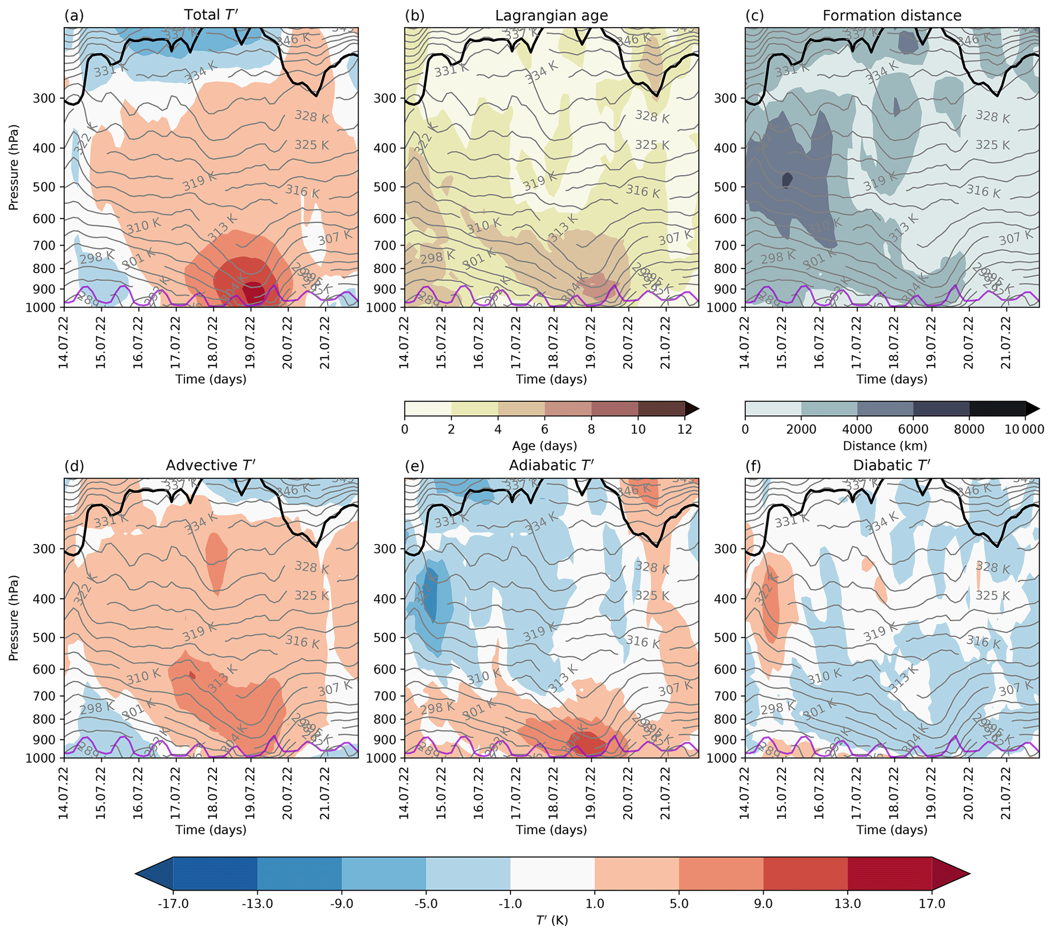
Finally, we turn our attention to the temporal evolution of the vertical T′ structure during the UK heatwave (Fig. 11). Interestingly, it bears some resemblance to that of the PNW heatwave (Fig. 5) and does feature some WCB characteristics preceding the peak period. Around 15 July, i.e. 1–2 d before the positive near-surface T′ started to form, positive T′ developed between 500 and 400 hPa. Figure 11 reveals that these T′ values consisted of positive diabatic T′ of +5 to +9 K (Fig. 11f), negative adiabatic T′ (Fig. 11e), and positive advective T′ (Fig. 11d), as well as comparatively long formation distances and large age values (Fig. 11b and c), which is reminiscent of the WCB signature during the PNW heatwave (Fig. 5). Much like during the PNW heatwave, upstream cloud diabatic heating and the associated WCB-like airstream thus helped to build up the ridge within which the UK heatwave ultimately occurred. Such WCB-induced ridge amplification is a common feature of heatwaves in this region (Zschenderlein et al., 2020). Moreover, the formation of positive T′ first at upper levels is consistent with an upper-level control on near-surface T′ (Zhang and Boos, 2023), although, as mentioned above, significant near-surface diabatic T′ was lacking in this case. From 16 July onwards, i.e. during the peak phase of the heatwave, the positive T′ above 700 hPa formed exclusively through advection. During this stage, the vertical T′ structure in the mid- to upper-troposphere thus resembled that of the RU heatwave more than that of the PNW heatwave.
The T′ peaked on 19 July at levels below 850 hPa (Fig. 11a). Interestingly, as for the PNW heatwave, the peak in adiabatic T′ propagated downward, and the peak in near-surface T′ coincided with the peak in positive adiabatic T′ at near-surface levels (Fig. 11e). Similar to the other two events, the T′ in the lowermost 300 hPa aged by about 2–4 d from 16 July to 19 July (Fig. 11b). Hereby, in the cross-sections shown in Fig. 11, the ageing of T′ (below 700 hPa) was co-located with the downward-propagating and amplifying peak in adiabatic T′. Finally, note that the ageing of T′ was confined predominantly to near-surface levels during both the RU and the UK heatwaves, which is in contrast to the PNW heatwave, where the ageing of T′ also occurred between 600 and 300 hPa.
The key difference between the UK heatwave and the other two events is, however, that at all levels, the diabatic T′ was small and mostly negative, except for the WCB-like signal between 500 and 300 hPa that preceded the near-surface heatwave. We interpret the lack of positive near-surface diabatic T′ as a result of the proximity of the UK heatwave region to the North Atlantic Ocean. Note that even climatologically, the diabatic T′ is near 0 during heat extremes in the UK and adjacent European coastal regions (Röthlisberger and Papritz, 2023a). This is because the respective (already anomalously warm) air is transported over ocean surfaces and is thereby cooled diabatically before arrival in these regions. That is, near-surface T′ during heat extremes that consist predominantly of adiabatic T′ and some advective T′ appear to be the norm for the UK and adjacent European coastal regions.
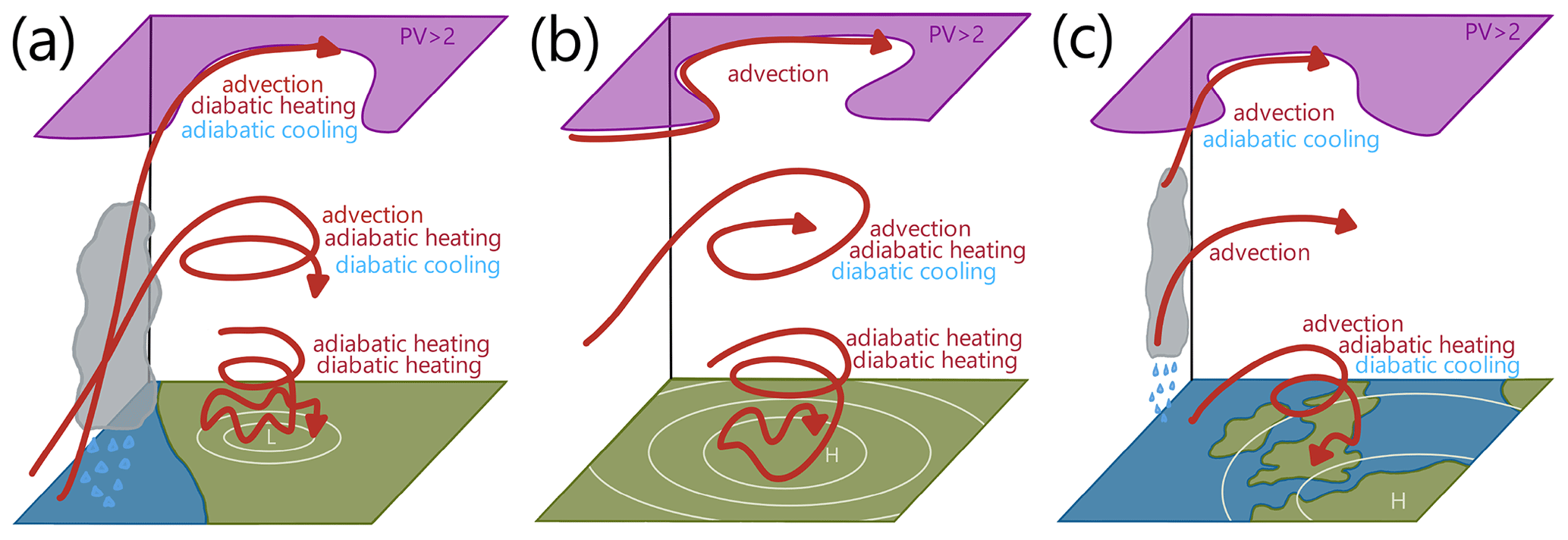
Figure 12Schematic of the (a) PNW, (b) RU, and (c) UK heatwaves. The three red lines in each of the panels depict the characteristics of air parcels ending up in the upper and middle troposphere, as well as in the boundary layer (the wriggling denotes the diurnal cycle). Processes acting to increase and decrease the ultimately positive T′ are denoted in red and blue font colour, respectively. The purple shading denotes stratospheric air.
Motivated by recent studies arguing for a top-down control on maximum near-surface temperatures during major heatwaves (Neal et al., 2022; Zhang and Boos, 2023), we have examined the detailed vertical temperature structure of three recent, record-shattering heatwaves that occurred in the Pacific Northwest in 2021 (PNW), western Russia in 2010 (RU), and western Europe in 2022 (UK). Hereby, a top-down control on the maximum near-surface T (and T′) through moist convective (in)stability is evident for the PNW and RU heatwaves, consistent with the theoretical arguments by Zhang and Boos (2023). This top-down control was less evident in the case of the UK heatwave, presumably due to weaker near-surface diabatic heating. To understand the physical causes of the vertical T′ structure during these three events, we employed the diagnostic framework of Röthlisberger and Papritz (2023a) and quantified the contributions to T′ of advection of air across climatological temperature gradients, adiabatic warming, and diabatic heating.
Our analyses reveal that all three heatwaves were characterised by bottom-heavy yet vertically deep positive T′ extending from the surface across the entire tropospheric column. The intensity of T′ and the underlying driving processes vary to a large degree in the vertical and from one case to the other (summarised in Fig. 12). Hereby, the differences across the three heatwaves relate to different synoptic storylines. The PNW heatwave was affected heavily by an upstream cyclone and its associated warm conveyor belt (WCB), which was instrumental in the amplification and poleward extension of the quasi-stationary ridge and also contributed significantly to upper-level T′ (Fig. 12a). In contrast, the anticyclone within which the RU heatwave formed was primarily affected by large-scale (dry) Rossby wave dynamics and experienced little upstream diabatic heating (Fig. 12b). The UK heatwave can perhaps be considered an intermediate case, where upstream cloud diabatic heating played some role in the early amplification of the anticyclone but was presumably not as dominant as in the PNW case.
Regarding the vertical structure of the T′ decomposition during the three heatwaves, our principal findings are as follows:
-
In all three cases, the composition of mid- and upper-tropospheric positive T′ differs substantially from that of lower-tropospheric positive T′. Mid- and upper-tropospheric positive T′ forms due to a combination of positive advective T′, resulting from the poleward advection of air from climatologically warmer regions and either near-zero adiabatic T′ and negative diabatic T′ or strongly negative adiabatic T′ and positive diabatic T′. The latter corresponds to the characteristic signature of upstream, strongly ascending WCB airstreams, which not only contribute to ridge amplification but are also a source of substantial T′ aloft. This WCB signature was particularly pronounced for positive mid- to upper-tropospheric T′ during the PNW heatwave, and our results thus now quantitatively support earlier studies that qualitatively argued for the importance of this WCB (Neal et al., 2022; Oertel et al., 2023). Moreover, a WCB also contributed to ridge amplification and positive upper-level T′ during the early phase of the UK heatwave, whereas in the case of the RU heatwave, such a signature was entirely absent. Adiabatic warming contributed notably to lower-tropospheric T′ during all three heatwaves, acting in conjunction with diabatically generated T′ in the case of the PNW and RU heatwaves.
-
Our results provide a nuanced view of the effect of vertical motion on T′ in anticyclones. While previous studies have argued that subsidence within anticyclones leads to positive T′ without specifying the vertical level (Pfahl and Wernli, 2012; Zschenderlein et al., 2019), we show that the net effect of vertical motion on T′ in the anticyclones leading to the three heatwaves is positive only in the lower 200–300 hPa of the atmosphere. Above that layer, the air does subside within the upper-level ridge. However, since a positive T′ already starts to form earlier while the air ascends – either quasi-isentropically or cross-isentropically if cloud formation occurs – a net negative effect of vertical motion on T′ results.
-
Amplification and downward propagation of adiabatic T′ were evident in both the PNW and the UK heatwaves, and near-surface T′ peaked when the maximum of adiabatic T′ reached near-surface levels. Subsequent studies should thus analyse a large number of major heatwaves to assess to what extent the timing of heatwave peaks is determined by the arrival of air with the largest positive adiabatic T′ in the boundary layer (as also observed for the PNW heatwave by Schumacher et al., 2022).
-
Finally, for all three cases, we find evidence of ageing of T′, in particular for lower-tropospheric air that subsided significantly before contributing to its respective heatwave. This result is fully consistent with the concept of a heat dome, within which air recirculates and accumulates heat. However the ageing of T′ alone does not directly imply recirculation of air but simply shows that the anomalies contributing to our events of interest became older throughout the course of the events.
The results of our study are limited in a number of ways. First, the total T′ is often the residual of partly opposing advective, adiabatic, and diabatic contributions. In those cases, it is difficult to determine which process should be considered to be the ultimate cause of the total T′, as the three processes are generally anti-correlated through their physical linkages (Röthlisberger and Papritz, 2023b). For cold extremes, Röthlisberger and Papritz (2023b) found that the most intense events, with the largest negative near-surface T′, occurred when these cancellations were particularly weak, i.e. when there was little damping of negative near-surface T′. A similar reasoning might also apply to near-surface T′ during hot extremes, and subsequent studies should thus examine more generally to what extent anomalously strong “forcing” (e.g. advection or dynamically induced subsidence) causes unusually large positive T′ and to what extent hot extremes result from attenuated (convective or other) damping mechanisms. Second, even though we use ERA5 data at a relatively high spatial and temporal resolution of 0.5° × 0.5° and 3 h, respectively, we cannot entirely assess to what extent the results of our trajectory calculations are resolution dependent. This particularly concerns all results and arguments related to boundary layer dynamics and convection, which clearly cannot fully be resolved at this resolution. However, while this is a caveat of our analysis, note that the spatial and temporal resolution used here is at least as high as that used in previous trajectory-based studies on heat extremes (e.g. Bieli et al., 2015; Quinting and Reeder, 2017; Zschenderlein et al., 2019; Schumacher et al., 2022). Third, our analyses focus almost entirely on T′, while for reaching moist convective neutrality the vertical humidity structure is also of obvious importance, which, according to Zhang and Boos (2023), thus also plays a role in limiting near-surface temperatures during major heatwaves. We fully acknowledge that subsequent studies should also assess the vertical moisture structure during major heatwaves and examine its causes.
Despite these caveats and a clear need for subsequent, more systematic studies on the atmospheric vertical structure during major heatwaves, our quantitative analysis of T′ profiles and their physical causes already yields considerable novel insights into the four-dimensional functioning of anticyclone–heatwave couples. It is thus hoped that these analyses will serve as a starting point for subsequent studies examining more systematically how large-scale dynamics, boundary layer processes, and convection act in concert to generate the most intense and most impactful heatwaves.
All results are based on the ERA5 reanalysis from ECMWF, which can be downloaded from the Copernicus Climate Service (https://climate.copernicus.eu/climate-reanalysis, Copernicus Climate Service, 2021). The LAGRANTO 2.0 code is freely available from Sprenger and Wernli (2015). The temperature anomaly decomposition was calculated by using code of Röthlisberger and Papritz (2023c) (https://doi.org/10.3929/ethz-b-000571107). Python scripts used to produce the analysis and visualisations are available from the authors upon request.
The supplement related to this article is available online at: https://doi.org/10.5194/wcd-5-323-2024-supplement.
BH performed the analyses and drafted the figures. MR and LP conceived the study. All three authors jointly interpreted the results and jointly wrote the paper.
At least one of the (co-)authors is a member of the editorial board of Weather and Climate Dynamics. The peer-review process was guided by an independent editor, and the authors also have no other competing interests to declare.
Publisher's note: Copernicus Publications remains neutral with regard to jurisdictional claims made in the text, published maps, institutional affiliations, or any other geographical representation in this paper. While Copernicus Publications makes every effort to include appropriate place names, the final responsibility lies with the authors.
We thank the ECMWF for providing access to the ERA5 reanalyses. Moreover, Heini Wernli (ETH Zürich) is acknowledged for his general support for this study. Furthermore, we thank the two reviewers for their constructive comments.
The contribution of Matthias Röthlisberger to this research has been supported by the H2020 European Research Council (grant no. 787652).
This paper was edited by Michael Riemer and reviewed by two anonymous referees.
Barriopedro, D., Fischer, E. M., Luterbacher, J., Trigo, R. M., and García-Herrera, R.: The hot summer of 2010: Redrawing the temperature record map of Europe, Science, 332, 220–224, https://doi.org/10.1126/science.1201224, 2011. a, b, c, d, e, f
Barriopedro, D., García-Herrera, R., Ordóñez, C., Miralles, D. G., and Salcedo-Sanz, S.: Heat waves: Physical understanding and scientific challenges, Rev. Geophys., 61, e2022RG000780, https://doi.org/10.1029/2022RG000780, 2023. a, b
Bieli, M., Pfahl, S., and Wernli, H.: A Lagrangian investigation of hot and cold temperature extremes in Europe, Q. J. Roy. Meteor. Soc., 141, 98–108, https://doi.org/10.1002/qj.2339, 2015. a, b, c, d, e, f
Conrick, R. and Mass, C. F.: The influence of soil moisture on the historic 2021 Pacific Northwest heatwave, Mon. Weather Rev., 151, 1213–1228, https://doi.org/10.1175/MWR-D-22-0253.1, 2023. a
Copernicus Climate Service: ERA5 reanalysis, Copernicus Climate Service [data set], https://climate.copernicus.eu/climate-reanalysis (last access: 17 July 2023), 2021. a
Dole, R., Hoerling, M., Perlwitz, J., Eischeid, J., Pegion, P., Zhang, T., Quan, X.-W., Xu, T., and Murray, D.: Was there a basis for anticipating the 2010 Russian heat wave?, Geophys. Res. Lett., 38, L06702, https://doi.org/10.1029/2010GL046582, 2011. a, b, c, d
Faranda, D., Pascale, S., and Bulut, B.: Persistent anticyclonic conditions and climate change exacerbated the exceptional 2022 European-Mediterranean drought, Environ. Res. Lett., 18, 034030, https://doi.org/10.1088/1748-9326/ACBC37, 2023. a
Fischer, E. M., Seneviratne, S. I., Vidale, P. L., Lüthi, D., and Schär, C.: Soil moisture–atmosphere interactions during the 2003 European summer heat wave, J. Climate, 20, 5081–5099, https://doi.org/10.1175/JCLI4288.1, 2007. a, b
Hauser, M., Orth, R., and Seneviratne, S. I.: Role of soil moisture versus recent climate change for the 2010 heat wave in western Russia, Geophys. Res. Lett., 43, 2819–2826, https://doi.org/10.1002/2016GL068036, 2016. a, b
Hermann, M., Röthlisberger, M., Gessler, A., Rigling, A., Senf, C., Wohlgemuth, T., and Wernli, H.: Meteorological history of low-forest-greenness events in Europe in 2002–2022, Biogeosciences, 20, 1155–1180, https://doi.org/10.5194/bg-20-1155-2023, 2023. a
Hersbach, H., Bell, B., Berrisford, P., Hirahara, S., Horányi, A., Muñoz-Sabater, J., Nicolas, J., Peubey, C., Radu, R., Schepers, D., Simmons, A., Soci, C., Abdalla, S., Abellan, X., Balsamo, G., Bechtold, P., Biavati, G., Bidlot, J., Bonavita, M., De Chiara, G., Dahlgren, P., Dee, D., Diamantakis, M., Dragani, R., Flemming, J., Forbes, R., Fuentes, M., Geer, A., Haimberger, L., Healy, S., Hogan, R. J., Hólm, E., Janisková, M., Keeley, S., Laloyaux, P., Lopez, P., Lupu, C., Radnoti, G., de Rosnay, P., Rozum, I., Vamborg, F., Villaume, S., and Thépaut, J.-N.: The ERA5 global reanalysis, Q. J. Roy. Meteor. Soc., 146, 1999–2049, https://doi.org/10.1002/qj.3803, 2020. a
Lau, W. K. M. and Kim, K.-M.: The 2010 Pakistan flood and Russian heat wave: Teleconnection of hydrometeorological extremes, J. Hydrometeorol., 13, 392–403, https://doi.org/10.1175/JHM-D-11-016.1, 2012. a, b, c, d
Meehl, G. A. and Tebaldi, C.: More intense, more frequent, and longer lasting heat waves in the 21st century, Science, 305, 994–997, https://doi.org/10.1126/science.1098704, 2004. a
Miralles, D. G., Teuling, A. J., van Heerwaarden, C. C., and de Arellano, J. V. G.: Mega-heatwave temperatures due to combined soil desiccation and atmospheric heat accumulation, Nat. Geosci., 7, 345–349, https://doi.org/10.1038/ngeo2141, 2014. a, b, c, d, e, f, g, h, i, j
Miralles, D. G., Gentine, P., Seneviratne, S. I., and Teuling, A. J.: Land–atmospheric feedbacks during droughts and heatwaves: state of the science and current challenges, Ann. N.Y. Acad. Sci., 1436, 19–35, https://doi.org/10.1111/nyas.13912, 2019. a
Neal, E., Huang, C. S. Y., and Nakamura, N.: The 2021 Pacific Northwest heat wave and associated blocking: Meteorology and the role of an upstream cyclone as a diabatic source of wave activity, Geophys. Res. Lett., 49, e2021GL097699, https://doi.org/10.1029/2021GL097699, 2022. a, b, c, d, e, f, g, h, i, j, k, l, m, n
Oertel, A., Pickl, M., Quinting, J. F., Hauser, S., Wandel, J., Magnusson, L., Balmaseda, M., Vitart, F., and Grams, C. M.: Everything hits at ance: How remote rainfall matters for the prediction of the 2021 North American heat wave, Geophys. Res. Lett., 50, e2022GL100958, https://doi.org/10.1029/2022GL100958, 2023. a, b, c, d, e
Papritz, L.: Arctic lower-tropospheric warm and cold extremes: horizontal and vertical transport, diabatic processes, and linkage to synoptic circulation features, J. Climate, 33, 993–1016, https://doi.org/10.1175/JCLI-D-19-0638.1, 2020. a
Pfahl, S. and Wernli, H.: Quantifying the relevance of atmospheric blocking for co-located temperature extremes in the Northern Hemisphere on (sub-)daily time scales, Geophys. Res. Lett., 39, L12807, https://doi.org/10.1029/2012GL052261, 2012. a, b, c
Philip, S. Y., Kew, S. F., van Oldenborgh, G. J., Anslow, F. S., Seneviratne, S. I., Vautard, R., Coumou, D., Ebi, K. L., Arrighi, J., Singh, R., van Aalst, M., Pereira Marghidan, C., Wehner, M., Yang, W., Li, S., Schumacher, D. L., Hauser, M., Bonnet, R., Luu, L. N., Lehner, F., Gillett, N., Tradowsky, J. S., Vecchi, G. A., Rodell, C., Stull, R. B., Howard, R., and Otto, F. E. L.: Rapid attribution analysis of the extraordinary heat wave on the Pacific coast of the US and Canada in June 2021, Earth Syst. Dynam., 13, 1689–1713, https://doi.org/10.5194/esd-13-1689-2022, 2022. a, b, c, d
Press Office: A milestone in UK climate history, MetOffice, https://www.metoffice.gov.uk/about-us/press-office/news/weather-and-climate/2022/july-heat-review (last access: 6 July 2023), 2022. a
Quinting, J. F. and Reeder, M. J.: Southeastern Australian heat waves from a trajectory viewpoint, Mon. Weather Rev., 145, 4109–4125, https://doi.org/10.1175/MWR-D-17-0165.1, 2017. a, b
Röthlisberger, M. and Martius, O.: Quantifying the local effect of Northern Hemisphere atmospheric blocks on the persistence of summer hot and dry spells, Geophys. Res. Lett., 46, 10101–10111, https://doi.org/10.1029/2019GL083745, 2019. a
Röthlisberger, M. and Papritz, L.: Quantifying the physical processes leading to atmospheric hot extremes at a global scale, Nat. Geosci., 16, 210–216, https://doi.org/10.1038/s41561-023-01126-1, 2023a. a, b, c, d, e, f, g, h, i, j, k, l, m, n, o, p, q
Röthlisberger, M. and Papritz, L.: A global quantification of the physical processes leading to near-surface cold extremes, Geophys. Res. Lett., 50, e2022GL101670, https://doi.org/10.1029/2022GL101670, 2023b. a, b, c
Röthlisberger, M. and Papritz, L.: Lagrangian Temperature Anomaly Decomposition for ERA5 Hot Extremes, ETH Research Collection [code], https://doi.org/10.3929/ethz-b-000571107, 2023c a
Röthlisberger, M., Frossard, L., Bosart, L. F., Keyser, D., and Martius, O.: Recurrent synoptic-scale Rossby wave patterns and their effect on the persistence of cold and hot spells, J. Climate, 32, 3207–3226, https://doi.org/10.1175/JCLI-D-18-0664.1, 2019. a
Santos, J. A., Pfahl, S., Pinto, J. G., and Wernli, H.: Mechanisms underlying temperature extremes in Iberia: A Lagrangian perspective, Tellus A, 67, 26032, https://doi.org/10.3402/tellusa.v67.26032, 2015. a
Schneidereit, A., Schubert, S., Vargin, P., Lunkeit, F., Zhu, X., Peters, D. H. W., and Fraedrich, K.: Large-scale flow and the long-lasting blocking high over Russia: Summer 2010, Mon. Weather Rev., 140, 2967–2981, https://doi.org/10.1175/MWR-D-11-00249.1, 2012. a, b
Schumacher, D. L., Hauser, M., and Seneviratne, S. I.: Drivers and mechanisms of the 2021 Pacific Northwest heatwave, Earths Future, 10, e2022EF002967, https://doi.org/10.1029/2022EF002967, 2022. a, b, c, d, e, f, g, h, i, j, k, l, m, n, o
Shepherd, T. G., Boyd, E., Calel, R. A., Chapman, S. C., Dessai, S., Dima-West, I. M., Fowler, H. J., James, R., Maraun, D., Martius, O., Senior, C. A., Sobel, A. H., Stainforth, D. A., Tett, S. F. B., Trenberth, K. E., van den Hurk, B. J. J. M., Watkins, N. W., Wilby, R. L., and Zenghelis, D. A.: Storylines: an alternative approach to representing uncertainty in physical aspects of climate change, Climatic Change, 151, 555–571, https://doi.org/10.1007/s10584-018-2317-9, 2018. a
Sousa, P. M., Trigo, R. M., Barriopedro, D., Soares, P. M. M., and Santos, J. A.: European temperature responses to blocking and ridge regional patterns, Clim. Dynam., 50, 457–477, https://doi.org/10.1007/s00382-017-3620-2, 2018. a
Sprenger, M. and Wernli, H.: The LAGRANTO Lagrangian analysis tool – version 2.0, Geosci. Model Dev., 8, 2569–2586, https://doi.org/10.5194/gmd-8-2569-2015, 2015. a, b
Stefanon, M., D'Andrea, F., and Drobinski, P.: Heatwave classification over Europe and the Mediterranean region, Environ. Res. Lett., 7, 014023, https://doi.org/10.1088/1748-9326/7/1/014023, 2012. a
Trenberth, K. E. and Fasullo, J. T.: Climate extremes and climate change: The Russian heat wave and other climate extremes of 2010, J. Geophys. Res.-Atmos., 117, D17103, https://doi.org/10.1029/2012JD018020, 2012. a, b
Vautard, R., Gobiet, A., Jacob, D., Belda, M., Colette, A., Déqué, M., Fernández, J., García-Díez, M., Goergen, K., Güttler, I., Halenka, T., Karacostas, T., Katragkou, E., Keuler, K., Kotlarski, S., Mayer, S., van Meijgaard, E., Nikulin, G., Patarčić, M., Scinocca, J., Sobolowski, S., Suklitsch, M., Teichmann, C., Warrach-Sagi, K., Wulfmeyer, V., and Yiou, P.: The simulation of European heat waves from an ensemble of regional climate models within the EURO-CORDEX project, Clim. Dynam., 41, 2555–2575, https://doi.org/10.1007/s00382-013-1714-z, 2013. a
Vicedo-Cabrera, A. M., de Schrijver, E., Schumacher, D. L., Ragettli, M. S., Fischer, E. M., and Seneviratne, S. I.: The footprint of human-induced climate change on heat-related deaths in the summer of 2022 in Switzerland, Environ. Res. Lett., 18, 074037, https://doi.org/10.1088/1748-9326/ace0d0, 2023. a
Wehrli, K., Guillod, B. P., Hauser, M., Leclair, M., and Seneviratne, S. I.: Identifying key driving processes of major recent heat waves, J. Geophys. Res.-Atmos., 124, 11746–11765, https://doi.org/10.1029/2019JD030635, 2019. a, b
White, R. H., Anderson, S., Booth, J. F., Braich, G., Draeger, C., Fei, C., Harley, C. D. G., Henderson, S. B., Jakob, M., Lau, C.-A., Admasu, L. M., Narinesingh, V., Rodell, C., Roocroft, E., Weinberger, K. R., and West, G.: The unprecedented Pacific Northwest heatwave of June 2021, Nat. Commun., 14, 727, https://doi.org/10.1038/s41467-023-36289-3, 2023. a, b, c
Xoplaki, E., González-Rouco, J. F., Luterbacher, J., and Wanner, H.: Mediterranean summer air temperature variability and its connection to the large-scale atmospheric circulation and SSTs, Clim. Dynam., 20, 723–739, https://doi.org/10.1007/s00382-003-0304-x, 2003. a
Yule, E. L., Hegerl, G., Schurer, A., and Schurer, A.: Using early extremes to place the 2022 UK heat waves into historical context, Atmos. Sci. Lett., 24, e1159, https://doi.org/10.1002/asl.1159, 2023. a
Zhang, X., Zhou, T., Zhang, W., Ren, L., Jiang, J., Hu, S., Zuo, M., Zhang, L., and Man, W.: Increased impact of heat domes on 2021-like heat extremes in North America under global warming, Nat. Commun., 14, 1690, https://doi.org/10.1038/s41467-023-37309-y, 2023. a
Zhang, Y. and Boos, W. R.: An upper bound for extreme temperatures over midlatitude land, P. Natl. Acad. Sci. USA, 120, e2215278120, https://doi.org/10.1073/pnas.2215278120, 2023. a, b, c, d, e, f, g, h, i, j, k, l, m, n, o, p, q
Zschenderlein, P., Fink, A. H., Pfahl, S., and Wernli, H.: Processes determining heat waves across different European climates, Q. J. Roy. Meteor. Soc., 145, 2973–2989, https://doi.org/10.1002/qj.3599, 2019. a, b, c, d, e, f, g, h
Zschenderlein, P., Pfahl, S., Wernli, H., and Fink, A. H.: A Lagrangian analysis of upper-tropospheric anticyclones associated with heat waves in Europe, Weather Clim. Dynam., 1, 191–206, https://doi.org/10.5194/wcd-1-191-2020, 2020. a
As in Röthlisberger and Papritz (2023a), tg is defined as the last trajectory time step for which has the same sign as , when moving along the trajectory backwards in time.