Changes in the North Atlantic Oscillation over the 20th century

The North Atlantic Oscillation explains a large fraction of the climate variability across the North Atlantic from the eastern seaboard of North America across the whole of Europe. Many studies have linked the North Atlantic Oscillation to climate extremes in this region, especially in winter, which has motivated considerable study of this pattern of variability. However, one overlooked feature of how the North Atlantic Oscillation has changed over time is the explained variance of the pattern. Here we show that there has been a considerable increase in the percentage of variability explained by the North Atlantic Oscillation (NAO) over the 20th century from 32 % in 1930 to 53 % by the end of the 20th century. Whether this change is due to natural variability, a forced response to climate change, or some combination remains unclear. However, we found no evidence for a forced response from an ensemble of 50 Coupled Model Intercomparison Project Phase 6 (CMIP6) models. These models did all show substantial internal variability in the strength of the North Atlantic Oscillation, but it was biased towards being too high compared to the reanalysis and with too little variation over time. Since there is a direct connection between the North Atlantic Oscillation and climate extremes over the region, this has direct consequences for both the long-term projection and near-term prediction of changes to climate extremes in the region.

1 Introduction

The North Atlantic Oscillation (NAO) is a pattern of variability in the sea level pressure over the North Atlantic associated with the subpolar low and subtropical high. The NAO is associated with large-scale changes in the position and intensity of both the storm track and the jet stream over the North Atlantic and thus plays a direct role in shaping atmospheric heat and moisture transport across the basin (Fasullo et al., 2020). It has also been shown that the NAO has a large impact on the Atlantic Meridional Overturning Circulation and thus oceanic heat transport and that this is largest on timescales of 20–30 years, leading to changes in Northern Hemisphere temperature of several tenths of a degree (Delworth and Zeng, 2016). The NAO has a positive and negative phase and exhibits considerable interannual variation between the two phases. The positive phase of the NAO indicates deeper-than-normal low pressure in the subpolar region and higher-than-normal high pressure over the subtropics. It is often associated with decreased temperature and precipitation anomalies over southern Europe and increased precipitation anomalies over northern Europe. The effects of the NAO are basin wide, and the positive phase is also associated with positive anomalies in temperature over the eastern United States. The opposite pattern and effects are seen during periods when the NAO is in its negative phase (Weisheimer et al., 2017).

It has long been established that the NAO dominates climate variability across a large part of the Northern Hemisphere from the eastern seaboard of North America across Europe to central Russia and from the Arctic in the north to the subtropical Atlantic (Hurrell et al., 2003). The NAO is an especially important component of the winter variability and has been linked to the frequency and intensity of climate extremes over Europe (Haylock and Goodess, 2004; Scaife et al., 2008; Fan et al., 2016). It is therefore essential to understand the scale of natural variability in the NAO, how the NAO responds to changes in external forcing, and whether these are captured in current climate models. If current climate models fail to capture either the natural variability or the response to forcing of the NAO, this could lead to a radically different projection of changes to climate extremes over Europe on the decadal to century timescales.

An index for the NAO is often identified in one of two ways. The first approach is to calculate the normalized difference in surface pressure between the subtropical high (Azores High) and subpolar low (Icelandic Low) over the North Atlantic sector. The second approach is to perform an empirical orthogonal function (EOF) analysis on sea level pressure over the North Atlantic region. An EOF analysis separates the variability in the sea level pressure into orthogonal modes, with the first mode containing the largest proportion of the variability and each subsequent mode containing progressively less. When an EOF analysis is used to calculate the NAO, the first mode indicates the NAO index, while the second and third modes usually provide the North Atlantic ridge and Scandinavian blocking patterns (Cassou et al., 2004).

An EOF produces two outputs, an eigenvalue and an eigenvector for each mode of variability. The eigenvector – or principal component (PC) as it is called – is a time series showing the variation in the mode in time, while the eigenvalue is a single value that quantifies how much of the variation in the original field is explained by the particular mode. Usually, the eigenvector is regressed back onto the original field to produce a map showing the pattern of variation associated with the mode, while the eigenvalue is weighted with all the eigenvalues to convert it to a percentage of the total variance explained by the given mode. Most studies using an EOF to examine the NAO focus on the eigenvector to highlight the pattern of variability, to examine the PC for signs of natural variability, or to study the changes in phase of the NAO as these relate directly to downstream weather changes. However, changes to the eigenvalue of each mode of variability have been largely overlooked in the literature. Changes to the eigenvalue tell us how the relative dominance of each mode has changed over time, either due to changes in the amplitude of the variability along the axis of a given mode or due to changes in the magnitude of the variability in other modes. A key question we wish to address is whether recent changes to the relative dominance of each of the modes of variability in the North Atlantic are due to changes in external forcing or natural variability. Given the strong influence of the NAO and other atmospheric modes of variability on regional climate in Europe, it is crucial to understand the role of natural variability and any forced response in order to make reliable predictions and projections of future changes to the NAO and hence climate extremes in these regions. In this study we focus on the eigenvalue and investigate how the percentage of variability explained by each mode has changed over time and how well the latest generation of climate models in the Coupled Model Intercomparison Project Phase 6 (CMIP6) capture this change. Since the NAO dominates the climate variability over the North Atlantic–European sector during the wintertime, we limit our study to the winter months, defined here as December–January–February (DJF).

2 Data sources

In this study we use monthly sea level pressure data from the European Centre for Medium-Range Weather Forecasts (ECMWF) Reanalysis of the 20th Century (ERA-20C;  Poli et al., 2016) and NOAA–CIRES (National Oceanic and Atmospheric Administration–Cooperative Institute for Research in Environmental Sciences) 20th Century Reanalysis (V2) (NOAA-20CR;  Compo et al., 2011), for the period of 1900 to 2010. The NOAA–CIRES 20th Century Reanalysis (V2) data are provided by the NOAA Physical Sciences Laboratory (PSL), Boulder, Colorado, USA, on their website at https://psl.noaa.gov (last access: 25 August 2021). The NOAA-20CR and ERA-20C reanalyses have horizontal resolutions of 2 and 1° respectively for the atmospheric fields.

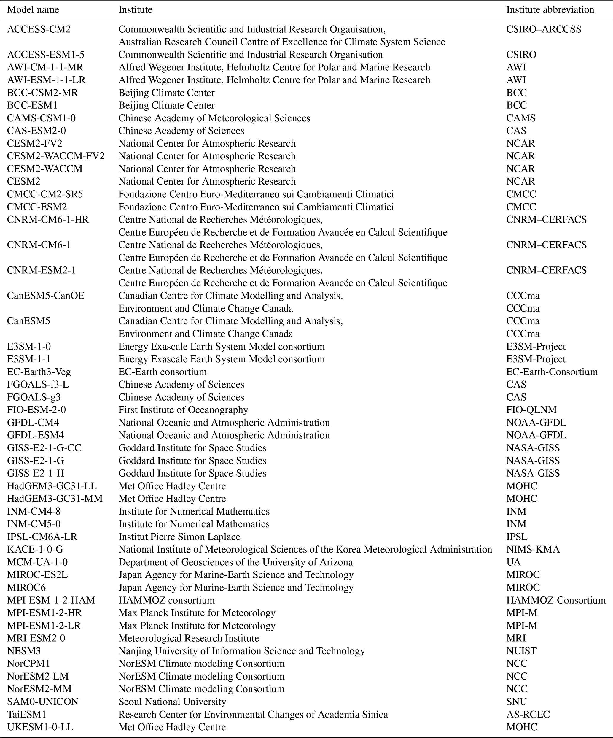
The climate model data analysed in this study come from the Coupled Model Intercomparison Project Phase 6 (CMIP;  Eyring et al., 2016), made publicly available through the Earth System Grid Foundation web portal at https://esgf-data.dkrz.de/ (last access: 30 June 2023). We use monthly averages of sea level pressure and precipitation flux from the historical simulations. The climate models analysed vary in horizontal resolution from 0.5° in the CNRM-CM6-1-HR model to approximately 2.5° in the MCM-UA-1-0 model. Since the common basis function method used in this study requires the climate model data to be on the same grid as the reanalysis used for the basis, the climate models were all interpolated to the 1° grid of the ERA-20C reanalysis using bilinear interpolation. We examine one ensemble member for each model, and the complete list of CMIP6 models examined in this study is given in Table 1.

Table 1 List of CMIP models and their respective modelling institutions.

3 Analysis

In this study, we use empirical orthogonal function analysis to identify the three primary modes of variability in sea level pressure in the ERA-20C and NOAA-20CR reanalyses. The first of these modes is considered to represent the North Atlantic Oscillation. We focus on the North Atlantic region, defined here as 20–80° N, 90° W–40° E (Fig. 1 inserts). The analysis is applied to a 30-year moving window over the full time period of 1900 to 2010, with the resulting time series plotted for the middle of each 30-year moving window, i.e. from 1915 to 1995. We use the “rule of thumb” proposed by North et al. (1982) to determine if a particular mode is distinct from neighbouring modes based on the separation of their eigenvalues compared to the standard error for their eigenvalues. Where the standard error overlaps the eigenvalue of another mode, both are considered to be blended modes and not independent.

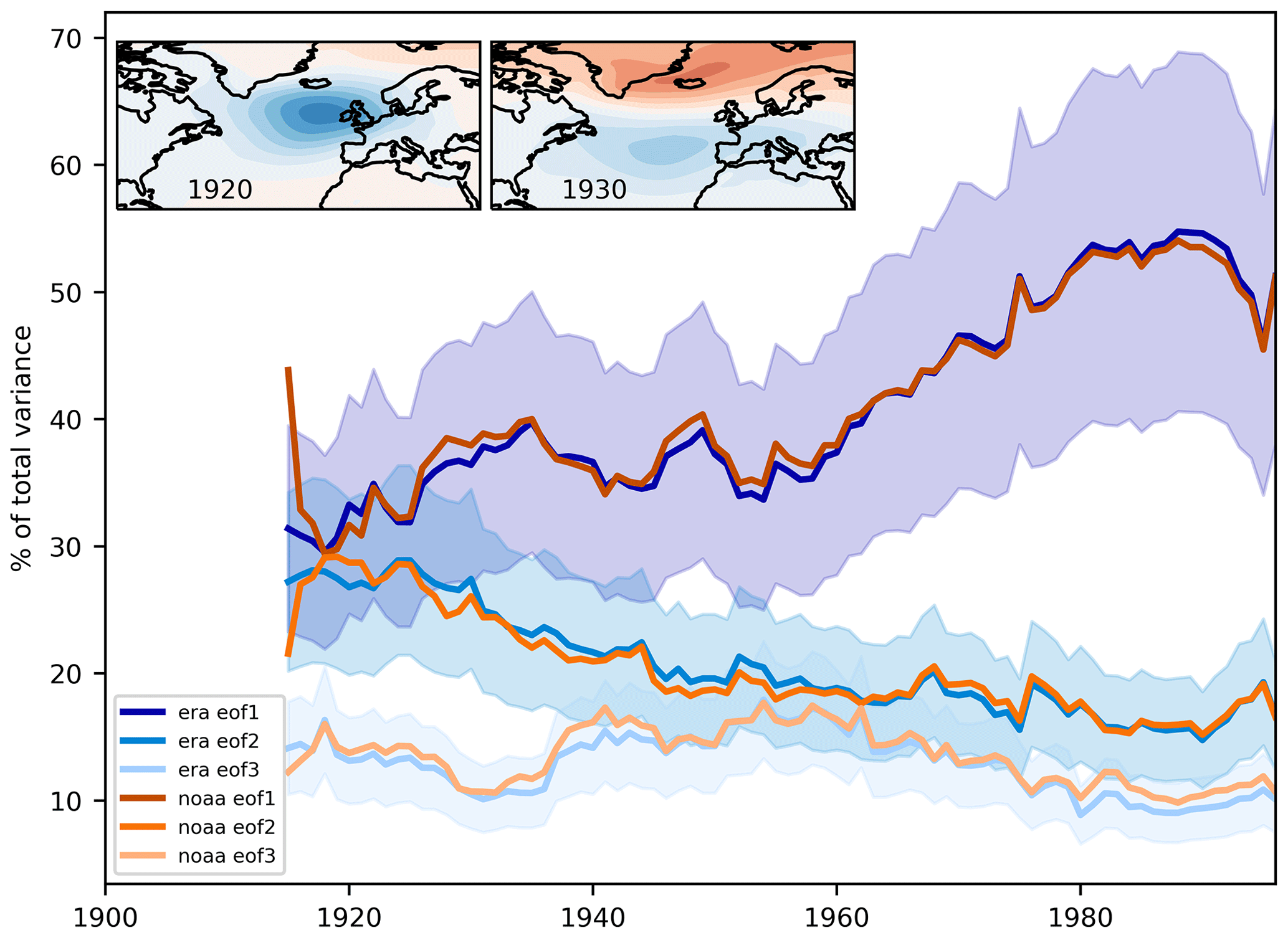
Figure 1 Percentage of variability explained by the first, second, and third modes in both ERA-20C (blue) and NOAA-20C (orange). The modes are shown from dark to light shades for modes 1 to 3 respectively. The inserts show the pattern in sea level pressure associated with the first mode of variability in ERA-20C for the 30-year periods centred on 1920 (left) and 1930 (right). The shading represents the error calculated using the North test to check the separation of the modes (North et al., 1982).

When attempting to compare EOF patterns from observations with those in models, two problems occur. Firstly, the modes may occur in a different order or may be different modes entirely; for example, the first mode in a particular model may not represent the NAO. Second, the modes may be inverted compared to the observations. While the second issue is easily resolved by identifying and inverting modes as needed, in this study we use an alternative approach to compared the modes called the common basis function (CBF;  Lee et al., 2019), which circumvents both of the above issues. The CBF approach projects model anomalies onto the EOFs of the reanalysis. This approach more directly addresses the question of how well the variability in a particular mode in the reanalysis is represented in the model. A more detailed explanation of the CBF approach is given in Lee et al. (2019) along with sensitivity testing of the method compared to the conventional EOF approach. The steps to apply the CBF approach are as follows.

1. Calculate an EOF from reanalysis and normalize it to unit variance.

2. Calculate the dot product of the spatial pattern of anomalies in the models and EOF pattern from reanalysis to get the unnormalized CBF PC time series.

3. Calculate the linear regression between the CBF PC and temporal anomalies at each grid point to obtain the slope of regression at each grid point.

4. Multiply regression slopes by the value of the CBF PC at each point to maximize the variance associated with the simulated expression of the reanalysis pattern.

5. Calculate the area-weighted mean of temporal variance at each grid point to derive the total variance explained by a given mode.

6. Multiply regression slopes by the standard deviation of the CBF PC to obtain the pattern of anomalies.

4 Results

The EOF analysis of sea level pressure in the ERA-20C and NOAA-20CR reanalyses using a 30-year moving window shows that the first three modes are very similar between the two reanalyses (Fig. 1). This emphasizes the robustness of the findings of how these modes have changed given that these two reanalysis products use different underlying models, spatial resolutions, and data assimilation methods and that there are also differences in the observations assimilated. Despite this they both capture the same change in the relative importance of the first three modes of variability in this region. In both reanalyses, the first mode rises from explaining approximately 32 % of the variability in the early 20th century to 53 % by the end of the century. Simultaneously, the second and third modes explain a decreasing percentage of the variability in North Atlantic sea level pressure, dropping from approximately 28 % to 16 % and from 14 % to 10 % for the second and third modes respectively. This shows a transference of variability explained from the North Atlantic ridge and Scandinavian blocking patterns into the NAO over the course of the 20th century. The bulk of the increase in the percentage of variability explained by the NAO occurs from the late 1950s onwards. This increase suggests that the NAO index has become a more valuable tool for explaining and/or predicting changes in climate over the North Atlantic and downstream over Europe in recent decades since the NAO has increased in the amount of variability in sea level pressure explained by the pattern.

It is clear from Fig. 1 that the first and second modes explained approximately the same amount of the variability in North Atlantic sea level pressure around 1920. When we examine the uncertainties using the North et al. (1982) rule of thumb, we find that the first mode is not distinct from the second mode until around 1930. The two inserts show the pattern associated with the first mode for the years 1920 and 1930. The 1930 pattern is the classical NAO pattern with a dipole of two centres of action, although they are spread horizontally due to the variation in the location of the centres of action over such a long time period. The pattern for 1920 shows a single centre of action to the west of the UK. This pattern matches with neither the NAO pattern nor the North Atlantic ridge pattern but is likely a merging of the two as the EOF analysis has not separated the modes correctly.

To explore how well this shift in the variability explained by the NAO is reproduced by the current generation of climate models, we use a CBF analysis on a 30-year moving window for each of the 50 CMIP6 models listed in Table 1. The CBF analysis uses the first principle component from the ERA-20C EOF analysis. Since PC1 is not clearly separated from PC2 until after 1930, we limit our analysis of the CMIP6 models to 1930 onward. The models do not in general reproduce the variation over time seen in the reanalyses, but this is to be expected since there is no matching of the phase of internal variability between the simulations or between the simulations and the reanalyses (Fig. 2). For example, the two versions of the Norwegian Earth System model (NorESM2) are the same model but run with a high or low resolution for the atmosphere and land components (∼ 1 and ∼ 2° respectively), yet they show very different trajectories over the 20th century. If the increase in the percentage of variability explained by the NAO seen in the reanalyses were the result of external forcing, such as a warming climate, the lack of a consistent trend or variation in the models would indicate that they fail to capture this response. This is highlighted by the multi-model mean which is approximately constant or even slightly decreasing over the 20th century. The lack of any consistent trend in the models supports the idea that the change in the percentage of variability explained is due to natural variability. In general, the climate models overestimated the percentage of variability explained by the NAO in the first half of the century and underestimated it in the second half, when compared to the reanalyses. While the time series shown in Fig. 2 were produced with a CBF analysis, a similar picture is obtained when examining the first mode of variability using an EOF analysis on each of the models independently (see Fig. S1 in the Supplement). The absolute variance explained is also very similar (Fig. S5).

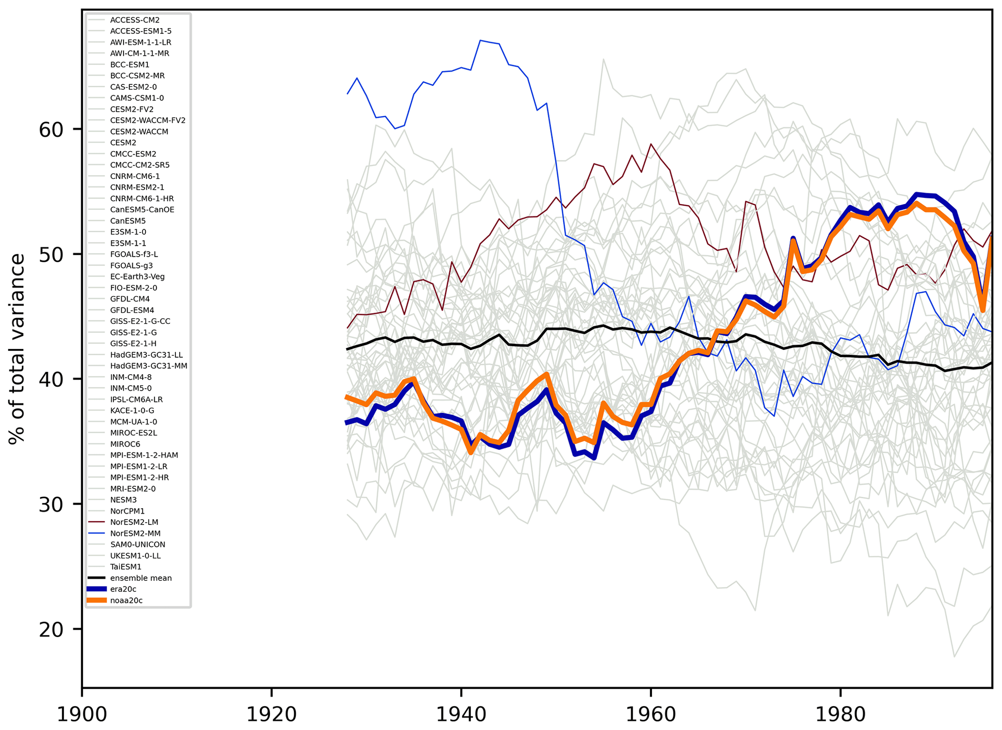
Figure 2 Percentage of variability explained by the first mode of the EOF in the reanalyses and the CBF in the CMIP6 models in a 30-year moving window. The ERA-20C and NOAA-20c reanalyses are shown in bold in blue and orange respectively. CMIP6 models are shown by thin lines in grey, except for NorESM2-LM (red) and NorESM2-MM (blue). Multi-model ensemble mean is shown as a thick black line.

If we accept that the increase in the percentage of variability explained seen in the reanalyses is due to natural variability, it is interesting to determine how well the models reproduce the range of explained variability compared to reanalysis. The climate models show a large range in the percentage of variability explained, from as low as 17 % in ACCESS-ESM1-5 to as high as 67 % in NorESM2-MM (Fig. 2). Of particular note are the NorESM2-LM and AWI-ESM-1-1-LR models that never drop below 44 % of the variability being explained by the NAO. The spread, as given by the interquartile range, in the percentage of variability explained in the ERA-20C reanalysis and individual models is shown in Fig. 3. Of the 50 models, 46 underestimate the spread when compared to reanalysis. NorESM2-MM is one of the few examples of a model having a greater spread than the reanalysis. This shows that the importance of the NAO pattern for explaining variations in North Atlantic sea level pressure is too consistent in the models and does not vary as much as in the reanalyses.

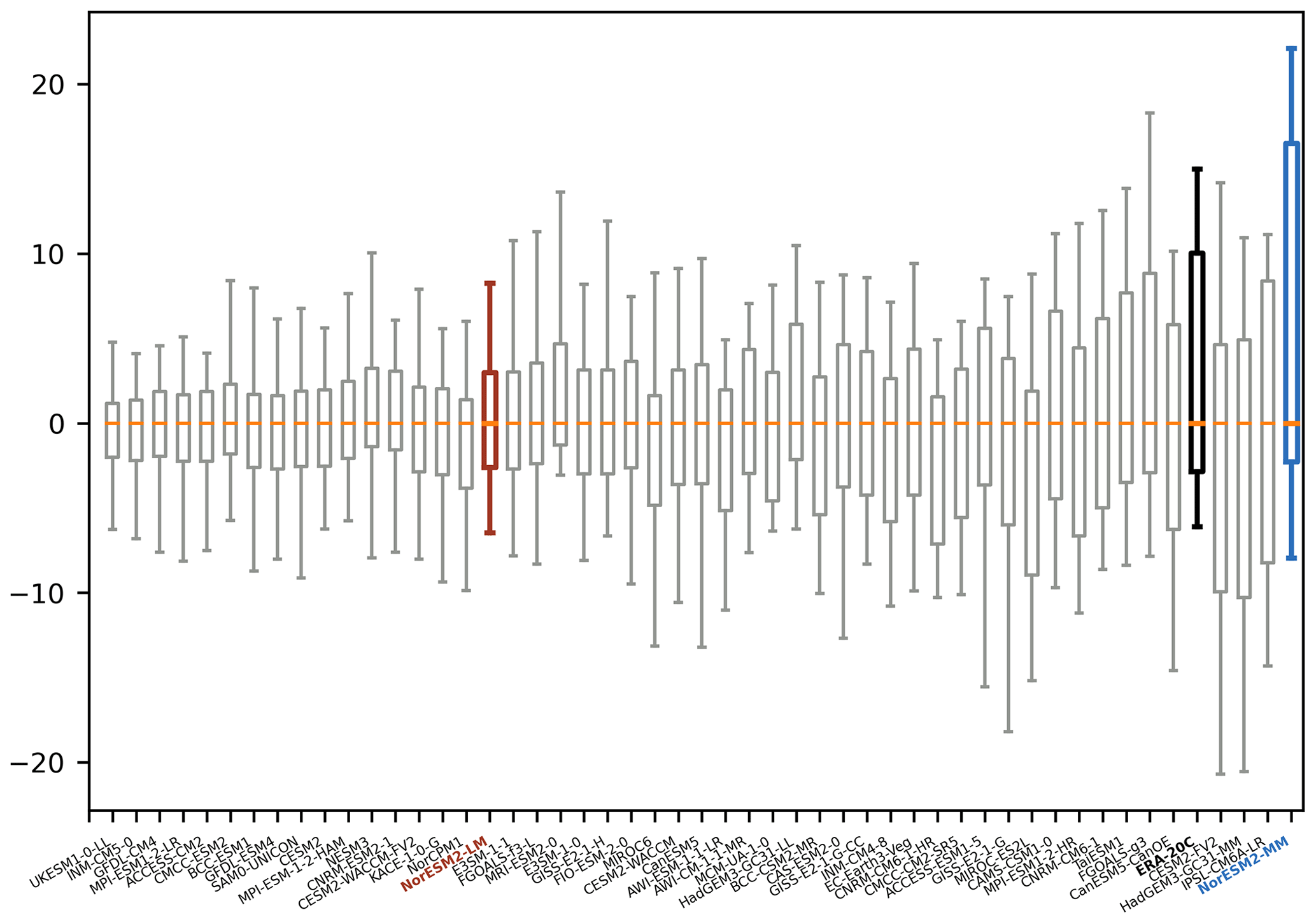
Figure 3 Spread in the percentage of variability explained by the first mode of the EOF in the reanalyses and the CBF in the CMIP6 models in a 30-year moving window, ranked in order of the interquartile range. Outlier points beyond 1.5 times the interquartile range beyond the upper and lower quartiles are not shown. The median has been subtracted from each model and from ERA-20C to align the spreads around a zero median, which allows for easier comparison of the spreads. ERA-20C is shown in black, and the CMIP models are shown in grey, except for NorESM2-LM (red) and NorESM2-MM (blue). The zero median for each model is highlighted in orange.

It is unclear from Fig. 2 if any individual model consistently produces an NAO similar to that found in the reanalyses. To explore this, we compared the percentage of variability explained, pattern correlation, and Taylor skill score between different 30-year periods. The results showed that there was no consistency between the different periods. For example, Fig. 4 shows the percentage of variability explained between the initial and final 30-year periods from Fig. 2. The models are ranked by the percentage of variability explained during the initial period, and there is no indication that this ordering is preserved in the later period. This highlights that large-scale patterns in models should not be compared to reanalyses or observations for individual periods, since a model that compares well to the observations during one period cannot be assumed to compare well during another period and any good comparison is the result of coincidental phasing of internal variability. Similar plots for the first and last 30-year periods are given for the percentage of variability explained, pattern correlation, and Taylor skill score in Figs. S2, S3, and S4 respectively.

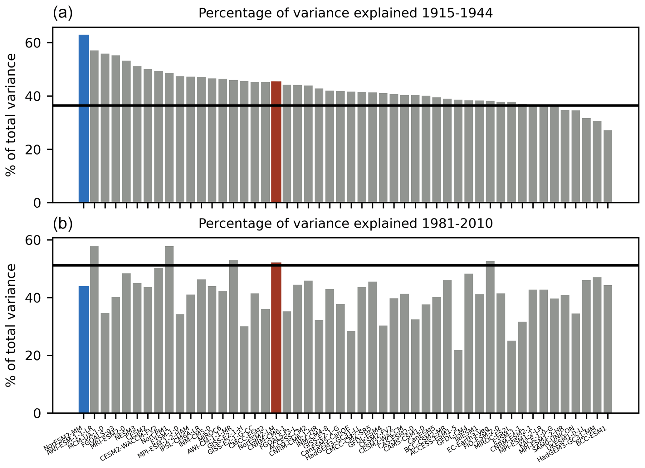
Figure 4 Percentage of variability explained by the first mode from the common basis function for each of the models in 30-year periods at the start and end of the full time series, 1915–1944 (a) and 1981–2010 (b). Models are ordered in both plots by the amount of variability explained for the initial period of 1915–1944. The horizontal black line in both plots gives the amount of variability explained by the first mode of the EOF in ERA-20C, upon which the CBFs are based. CMIP6 models are shown in grey, except for NorESM2-LM (red) and NorESM2-MM (blue).

Given the increase in the percentage of variability in sea level pressure explained by the NAO found in the reanalyses, it is of interest to see how the variability in sea level pressure itself has changed over the same period. Figure 5 shows the area-weighted mean variance in sea level pressure over the North Atlantic region for a 30-year moving window in both the two reanalyses and the 50 CMIP6 models. The reanalyses show a general increase, especially after 1950, rising from approximately 800 hPa at the beginning of the century to approximately 1000 hPa by the end of the century. This is equivalent to the standard deviation in sea level pressure changing from approximately 28 to 31 hPa. This indicates a small but steady increase in either the depth or the frequency of low-pressure systems moving along the North Atlantic storm tracks (Feser et al., 2014).

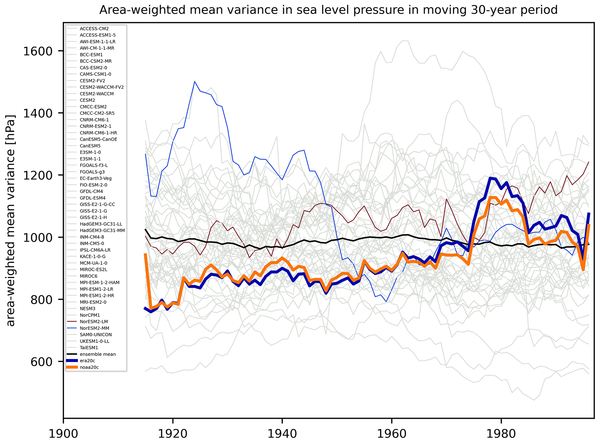
Figure 5 Area-weighted mean variance in sea level pressure in a 30-year moving window. The ERA-20C and NOAA-20c reanalyses are shown in bold in blue and orange respectively. CMIP6 models are shown by thin lines in grey, except for NorESM2-LM (red) and NorESM2-MM (blue). Multi-model ensemble mean is shown as a thick black line.

The climate models show quite a different picture, with a large spread in the variability in sea level pressure, ranging from 475 hPa in INM-CM4-8 to 1633 hPa in IPSL-CM6A-LR. This suggests that some models have too few or weaker low-pressure systems, while others have too many or deeper low-pressure systems compared to the reanalyses. It is interesting to note the similarities between the changes in sea level pressure variance and variance explained by NAO in both the models and reanalyses (cf. Figs. 5 and 2). For example, NorESM2-MM shows high values in both plots until the 1940s, when it drops to more moderate values and remains approximately constant until the end of the century. This means that the change in the sea level pressure variance associated with the NAO pattern over this period is even larger than would be assumed from Fig. 2. The absolute variance explained is shown in Fig. S5, a combination of the total variance in the sea level pressure shown in Fig. 5 and the percentage of variability explained.

5 Conclusions

In this study we have examined how the percentage of variability in sea level pressure explained by the North Atlantic Oscillation pattern has increased over the 20th century, while the percentage of variability explained by the second and third modes has decreased. The latest generation of climate models do not reproduce this change, suggesting that the observed change is not the result of external forcing such as a warming of the climate but is due to internal variability. However, most of the models also underestimate the spread in explained variance when compared to the reanalyses, indicating that the relative strength of the NAO is too persistent in the models. Examination of the variance in sea level pressure shows that the models have a greater spread than is seen in the reanalyses, suggesting that the low-pressure systems are too few or too weak in some models and too strong or too deep in others. Given that the range of variability explained in the models is comparable to the change in variability explained in the reanalyses and that the models show a wide range of responses over the 20th century despite all being forced by the same historical forcings, we suggest that the increase in the percentage of variability explained is driven by natural variability and is not a forced response. If the changes to the relative importance of the NAO seen in the reanalysis are indeed purely due to natural variability, then this has direct implications for the ability of climate models to capture natural variability in climate extremes over Europe. It is also crucial that multi-decadal prediction of changes to climate extremes over Europe account for the phase of natural variability in the relative strength of the NAO.

An alternative possibility is that the changes seen in the reanalyses are a combination of natural variability and a forced response that is not represented in CMIP6 models. This might explain why the models are systematically biased towards underestimating the variability in the explained variance of the NAO, as seen in Fig. 3. If part of these changes in the relative strength of the NAO are indeed due to a forced response that is lacking in climate models, then there is a risk of a systematic underestimation of the changing risks of climate extremes over Europe in a warming world. A second alternative is that the change is the results of a long-term, multi-decadal variability (perhaps with a variability of 60–80 years such as that found in studies on Bjerknes compensation). If the models reproduced such oscillations and were initialized in different phases of the multi-decadal signal, this could possibly produce the observed differences in the long-term changes in variance explained by the NAO. However, it would be very difficult to reliably confirm a 60–80-year oscillation in a 150-year simulation since you would barely have two full cycles. Both of these alternatives are speculation and would need significant further investigation to confirm.

While the large-scale patterns derived using an EOF analysis are a good indicator of the changes in weather systems over the North Atlantic, recent works have found that jet regimes are better at capturing spatial structure compared to patterns like the NAO and have the advantage of a greater physical connection to the underlying weather systems (Madonna et al., 2021). Future work is planned to investigate how these jet regimes have varied over time in the reanalyses and how well the CMIP6 models capture these variations.