Large-ensemble assessment of the Arctic stratospheric polar vortex morphology and disruptions

The stratospheric polar vortex (SPV) comprises strong westerly winds during winter in each hemisphere. Despite ample knowledge on the SPV's high variability and its frequent disruptions by sudden stratospheric warmings (SSWs) in the Northern Hemisphere (NH), questions on how well current climate models can simulate these dynamics remain open. Specifically the accuracy in reproducing SPV morphology and the differentiation between split and displacement SSW events are crucial to assess the models in this regard. In this study, we evaluate the capability of climate models to simulate the NH SPV by comparing large ensembles of historical simulations to ERA5 reanalysis data. For this, we analyze geometric-based diagnostics at three pressure levels that describe SPV morphology. Our analysis reveals that no model exactly reproduces SPV morphology of ERA5 in all diagnostics at all altitudes. Concerning the SPV morphology as stretching (aspect ratio) and location (centroid latitude) parameters, most models are biased to some extent, but the strongest deviations can be found for the vortex-splitting parameter (excess kurtosis). Moreover, some models underestimate the variability of SPV strength. Assessing the reliability of the ensembles in distinguishing SSWs subdivided into SPV displacement and split events, we find large differences between the model ensembles. In general, SPV displacements are represented better than splits in the simulation ensembles, and high-top models and models with finer vertical resolution perform better. A good performance in representing the morphological diagnostics does not necessarily imply reliability and therefore a good performance in simulating displacements and splits. Assessing the model biases and their representation of SPV dynamics is needed to improve credibility of climate model projections, for example, by giving stronger weightings to better performing models.

1 Introduction

In winter the dynamics of the mid-latitude and polar stratosphere are dominated by the stratospheric polar vortex (SPV). The SPV is a circumpolar band of usually strong westerly winds, forming in autumn due to the cooling of the polar stratosphere. When the stratosphere warms again in spring, the temperature gradient reverses and easterly winds prevail during summer (Holton, 1980). The SPV affects the concentration of ozone over the poles: strong winds are accompanied by lower-than-average temperatures, allowing the formation of polar stratospheric clouds, where ozone-depleting substances are activated (Langematz et al., 2014; Lawrence et al., 2020). Via stratosphere–troposphere coupling (Baldwin and Dunkerton, 2001), the SPV can influence tropospheric circulation patterns, temperatures and precipitation (Thompson et al., 2002; Butler et al., 2017; King et al., 2019). Hence, uncertainties associated with the representation of the SPV in models relate to uncertainties in tropospheric climate projections, in particular with the position of the jet and the precipitation patterns over Europe and the Mediterranean region (Scaife et al., 2012; Zappa and Shepherd, 2017), as well as with sea level pressure over the Arctic (Simpson et al., 2018). Especially in the Northern Hemisphere (NH), where the SPV is highly variable (Baldwin et al., 2021), the strongest changes happen during so-called sudden stratospheric warmings (SSWs). SSWs are abrupt warmings of the stratosphere usually connected with zonal mean zonal wind drop at middle to high latitudes. During a so-called major SSW, the wind even reverses to easterly. In the NH, SSWs occur on average about six times per decade (Charlton and Polvani, 2007; Karami et al., 2023). They are much less frequent in the Southern Hemisphere, with only one recorded major SSW in 2002 since the beginning of the satellite era (Jucker et al., 2021). SSWs can be categorized into two different kinds. Either the SPV is split into two separate vortices or it is displaced to lower latitudes (Charlton and Polvani, 2007). It is still a matter of current research whether the pressure patterns before the event and especially the surface pressure response after the event are different depending on SSW type (Mitchell et al., 2013; Seviour et al., 2013; Maycock and Hitchcock, 2015).

Multiple studies have focused on analyzing whether climate change alters stratospheric dynamics (Manzini et al., 2014; Ayarzagüena et al., 2020; Rao and Garfinkel, 2021). In the model simulations of the Climate Model Intercomparison Project Phase 5 (CMIP5), the largest uncertainty between individual models regarding a change of stratospheric wind speeds is found at 60° N and 10 hPa (Manzini et al., 2014), the region where the SPV strength and SSWs are commonly diagnosed (Charlton and Polvani, 2007). In line with this uncertainty, there is no agreement among CMIP5 and CMIP6 models on a trend in SSW frequency (Ayarzagüena et al., 2018; Rao and Garfinkel, 2021). The multi-model mean suggests a slight SSW frequency increase, but the inter-model spread is large, even in the historical simulations (Rao and Garfinkel, 2021). Ayarzagüena et al. (2018) used 12 Chemistry-Climate Model Initiative (CCMI) models for their analysis and found that most of them do not project a significant SSW frequency trend. Seviour et al. (2016) used two-dimensional SPV diagnostics to differentiate between vortex splits and displacements and found that most CMIP5 models show some bias in simulating SSWs. Hall et al. (2021) made similar findings with CMIP6 models and found no notable improvement compared to CMIP5. Differences in the chemistry schemes of the models, in the mean SPV strengths and in upward-propagating wave activity flux (Wu and Reichler, 2020) have been identified as possible reasons for the large spread in SSW frequency and its trends. The large inter-model spread and the uncertainties in the SPV response to climate change underline the need to investigate the reliability of climate models in simulating the SPV. This includes its form, strength and stability. Most previous multi-model studies only used a single run from each climate model. However, single-model realizations limit possibilities in attributing model differences to the underlying physics or to natural variability (Blanusa et al., 2023; Deser et al., 2020). Particularly the highly variable wintertime NH stratosphere requires analysis using large ensemble sizes (Deser et al., 2020). Hence, we limit our analysis to the NH SPV.

Therefore, we here assess the reliability of recent large-ensemble model simulations in representing the SPV and its spatial variability. For this, after introducing our methods in Sect. 2 we compare in Sect. 3 geometric SPV diagnostics in large climate model ensembles with ERA5 reanalysis data using rank histograms (Matthewman et al., 2009; Seviour et al., 2013). Furthermore, the reliability of the ensembles in detecting SSWs separated into SPV splits and displacements is analyzed in Sect. 4. In Sect. 5 we discuss our results with regard to possible reasons for the detected model differences, and we finish the paper with some concluding remarks in Sect. 6.

2 Methods

2.1 Data

For this climate model assessment on SPV strength, form and stability, we use large climate model simulation ensembles. Each ensemble consists of multiple simulation members, which only differ by modified initial conditions, while the model physics and setups are identical (Deser et al., 2020). In our analysis, we use climate models from the Multi-Model Large Ensemble Archive (MMLEA) provided by the US CLIVAR (Climate and Ocean – Variability, Predictability, and Change) working group on large ensembles (Deser et al., 2020) as well as ensembles from the Coupled Model Intercomparison Project Phase 6 (CMIP6, Eyring et al., 2016). We use the historical simulations of those ensembles where all CMIP5- and CMIP6-class historical forcings are included. Information about the 11 climate models used in our analysis are provided in Table 1. The selection criteria for our model database were, firstly, availability of at least 10 ensemble members and, secondly, availability of the geopotential height at the pressure levels 10, 50 and 100 hPa to calculate the SPV moment diagnostics (see Sect. 2.2). GFDL-CM3 is an exception as these model data were available only at 100 hPa. For reference, we compare the historical simulation ensembles with ERA5 reanalysis data (Hersbach et al., 2020). In this regard, we emphasize that ERA5 is designated as a state-of-the-art benchmark regarding its extensive horizontal and vertical resolution compared to other reanalyses (Hoffmann and Spang, 2022). We apply the same geopotential height-based SPV diagnostics to the ERA5 reanalysis that we also apply to the model ensemble data. The analysis is carried out for the period 1979–2014 covering years when, among others, satellite observations were assimilated to ERA5 (Hersbach et al., 2020). Vokhmyanin et al. (2023) found 22 SSWs in these 36 years of ERA5 data. We analyze daily data of the months from November through March in the NH, as this is when the SPV is usually present and SSW disruptions happen.

Kirchmeier-Young et al. (2017)Swart et al. (2019)Danabasoglu et al. (2020)Voldoire et al. (2019)Donner et al. (2011)Volodin and Gritsun (2018)Boucher et al. (2020)Tatebe et al. (2019)Olonscheck et al. (2023)Müller et al. (2018)Sellar et al. (2019)

Table 1 Analyzed climate model ensembles from CMIP5 and CMIP6. Low-top models are above and high-top models are below the horizontal line.

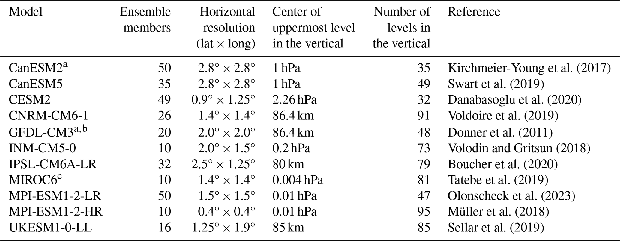
^a Model is part of CMIP5; other models are part of CMIP6. Only UKESM1-0-LL and CNRM-CM6-1 include full interactive chemistry; CNRM-CM6-1 has a simplified interactive chemistry scheme; the other models are run in dynamics-only mode. ^b Model data are only available at 100 hPa. ^c Model is available for 10 ensemble members only. All 50 ensemble members only cover monthly mean data (Shiogama et al., 2023).

2.2 Polar vortex moment diagnostics

To assess spatiotemporal SPV characteristics, the following two-dimensional moment diagnostics are calculated (for details of the calculation see Matthewman et al., 2009; Seviour et al., 2013).

• The aspect ratio, i.e., the ratio of the major to the minor axis of the SPV ellipse, diagnoses how stretched the SPV is. $\mathrm{High}/\mathrm{low}$ aspect ratio values indicate a stretched/circular SPV, and exceptionally high values are often associated with SPV disturbances such as SSWs.

• The excess kurtosis is a measure for the distribution of geopotential height values inside the SPV; constant geopotential height values lead to an excess kurtosis of 0. A low geopotential height center, i.e., a stable SPV, is represented by high kurtosis values, and two separated areas of low geopotential height, i.e., a vortex split, are indicated by a negative kurtosis.

• The SPV location is diagnosed by centroid latitude and longitude. A lower centroid latitude is often associated with a disrupted SPV and can indicate a displacement; centroid longitude values can additionally help determine the SPV position.

• The objective SPV area is an indicator of the SPV strength, as a large area of low geopotential height is often connected with high wind speeds.

More detailed descriptions are provided in Sect. S2. In contrast to Matthewman et al. (2009), who described their method using potential vorticity, we here use the geopotential height to define the SPV edge, as suggested by Seviour et al. (2013). For this, the algorithms from Seviour et al. (2013) have been modified accordingly; the updated versions can be accessed from Kuchar and Öhlert (2024).

2.3 Rank histograms

The rank histogram (RH) is a tool used in ensemble forecast verification to determine the reliability of ensemble forecasts and to diagnose errors in their mean and spread. RHs consist of n+1 bins, where n is the number of model ensemble members. For each time step and variable, the ensemble values are sorted in ascending order, and the ERA5 reanalysis value at that particular time step is placed into this set at position k. The histogram shows counts of all bins greater than or equal to k. This procedure is repeated for each time step (for details of the calculation see Hamill, 2001; Wilks, 2011). For a reliable (calibrated) ensemble, the counts should be uniformly distributed over all bins. If the ensemble deviates from the reanalysis, the shape of the histogram can be used to find out why (Wilks, 2011). For example, if the historical simulations are biased, there will be a linear trend in the histogram. When the counts of the bins are higher on the left (lower bins) and lower on the right (higher bins) of the histogram, the ensemble simulates the variable to be consistently higher than the observed values, which is called overforecasting bias. The opposite would be an underforecasting bias. If the ensemble underestimates/overestimates the variability, the ranks at the edges of the histogram have higher/lower counts than in the center, which is called underdispersion/overdispersion.

For an objective assessment of the results, we consider an additional diagnostic in our study, namely the χ² statistic. This diagnostic quantifies how close the RH is to an ideal uniform distribution. A perfectly flat histogram would produce a χ² value of 0. Jolliffe and Primo (2008) introduced a method to split the χ² statistic into multiple metrics, where each one describes a certain histogram shape. The linear trend is used as a bias indicator. A U-shaped RH indicates underdispersion (ensemble spread is too low). On the contrary, RH with the shape of central dome indicates that the ensemble spread is too broad. These metrics can be especially helpful when both bias and over- or underdispersion are present in an ensemble, as this can be difficult to distinguish visually from the RH alone. The contributions of these two components to the total χ² statistic are presented along all RHs in our assessment. These statistics should serve in relation to the other models instead of defining any threshold for a “good” or “bad” model.

2.4 Perfect model range

Due to internal variability, it is possible that a RH has a somewhat uneven distribution. To determine which deviations from a uniform distribution can be attributed to internal variability, Suarez-Gutierrez et al. (2021) suggested the use of “a perfect model range”. To obtain this range, a rank histogram is created for each ensemble member where this specific member is treated as a reference (i.e., as if it was the reanalysis). This results in slightly different values for each bin in the RHs, depending on the member in question. The perfect model rank range is then defined by the range where 90 % (5th–95th percentile) of the bin counts are found. Since a member from the ensemble can never be higher or lower than all ensemble members, the values for the rank range in the first and last bin are ignored.

2.5 SSW diagnostics

SSW events can be subdivided into SPV splits and displacements and can be detected by means of the metrics described above. As suggested by Seviour et al. (2013), we detect SPV splits by an aspect ratio higher than 2.4. For a displacement, the centroid latitude is arguably the best indicator. Here, as defined by Seviour et al. (2013) a displacement is detected if the centroid latitude is lower than 66° N.

To assess how well the probability of these events is represented in the model simulation ensembles, the receiver operating characteristic (ROC) curves are used (see Figs. S1 and S2 and their description in Sect. S3). The area under the ROC curve (AUC) indicates how well an ensemble is able to discriminate between SSW and non-SSW events using the thresholds above (with reference to ERA5). AUC ranges from 0 to 1. Values of 1, 0.5 and 0 indicate perfect skill, random guessing and no skill, respectively. As an example, we show ROC for displacements and splits in Fig. 2 for the CanESM5 ensemble. Bin values indicated along ROC are probabilities of whether the model simulates displacements and splits across its ensemble members, respectively. These values then serve as inputs for the calculation of dichotomous contingency tables which includes true and false-positive rates displayed on the y and x axis, respectively. Therefore, there is no assumption about the temporal correspondence of these events, but the probability distributions between ERA5 and model ensembles are assessed. Fig. 2b demonstrates that CanESM5 cannot discriminate split events better than random guessing (see Sect. 4.2). To determine the uncertainty of the AUC, we provide error bars using the approach of the perfect model range, where we assume each ensemble member is an observation.

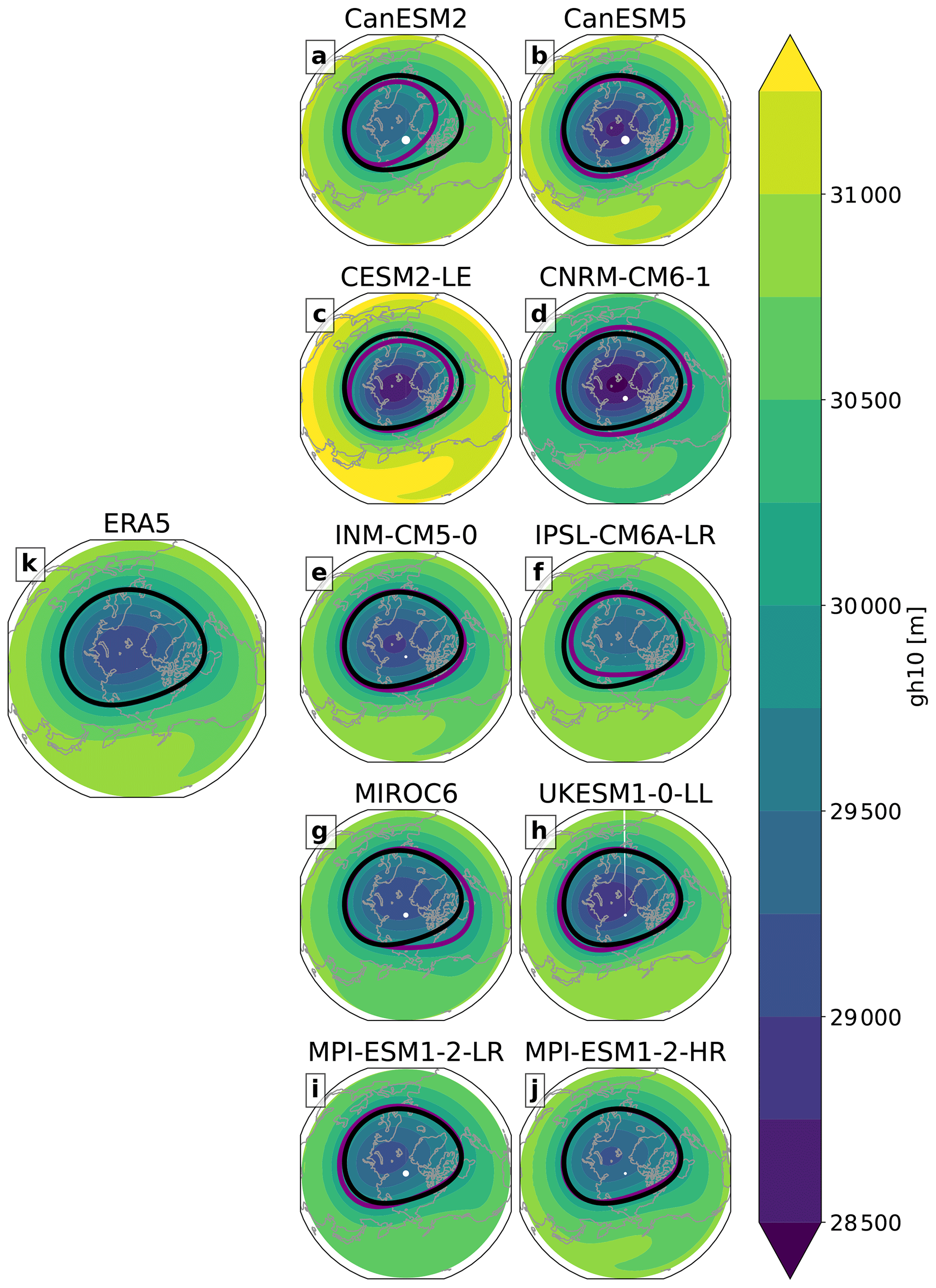
Figure 1 Geopotential height climatology at 10 hPa (gh10) of all analyzed model ensembles: CanESM2 (a), CanESM5 (b), CESM2 (c), CNRM-CM6-1 (d), INM-CM5-0 (e), IPSL-CM6A-LR (f), MIROC6 (g), UKESM1-0-LL (h), MPI-ESM1-2-HR (i), MPI-ESM1-2-LR (j), and ERA5 (k) for the period 1979–2014. The black and purple lines represent the contours of 30 000 m in ERA5 and in the particular model, respectively.

Figure 2 Receiver operating characteristic (ROC) curves for displacements (a) and splits (b) in CanESM5. Bin values indicated along ROC are probabilities of whether the model simulates displacements and splits across its ensemble members, respectively. Area under the ROC curve (AUC) is visualized and also specified in the figure. The dashed line represents random discrimination skill, i.e., AUC = 0.5.

We also reproduce the methodology to detect displacement and split SSWs from Hall et al. (2021) as previously applied in Mitchell et al. (2011) and based on Seviour et al. (2013) to examine relationships between modal centroid latitude and aspect ratio and displacement and split SSW frequency, respectively. The frequencies of ERA5 SSW split and displacement events determined with this method are within the uncertainty of other methods (∼ 6.94 events per decade; ∼ 6.66 events per decade including displacement and splits events only; displacement $/$ split ratio is equal to 1.4; Gerber et al., 2022). Using this methodology, we provide the list of ERA5 SSW split and displacement events in Table S2 to document this agreement.

3 Analysis of geometric polar vortex diagnostics

We show the geopotential height climatology at 10 hPa (gh10) of all analyzed model ensembles and ERA5 for the period 1979–2014 in Fig. 1. The figure shows that some models do not simulate gh10 well in comparison to ERA5 (CanESMs, CESM2). On the other hand, the visual resemblance between ERA5 and other models (e.g., UKESM1-0-LL) can clearly be seen, too. However, details about the reliability of these large-ensemble model simulations in representing the SPV and its spatial variability cannot be decomposed based on such depictions. Hence, moment diagnostic analyses are needed to shed light on the SPV and its properties in large-ensemble simulations.

In the following, the agreement between the ERA5 reanalysis and the historical simulations of the climate model ensembles will be compared by means of the SPV moment diagnostics introduced in Sect. 2.2. For this, RHs are discussed for all available models at 10, 50 and 100 hPa; however, the figures for 50 hPa and for 100 hPa are shown in the Supplement. We also summarize bias and spread from these figures in Table S1.

3.1 Aspect ratio

The aspect ratio of the SPV is determined by the ratio of the major to the minor ellipse axis. Thus, it measures how stretched the SPV is, providing high values of aspect ratio for stretched SPVs and low values for more circular SPVs. Figure 3 shows RHs of the aspect ratio for all analyzed climate model ensembles together with the above introduced statistical values χ², bias and spread at 10 hPa, the level that is most commonly used to detect SPV splits. As indicated in Sect. 2, the interpretation of all results here is with reference to ERA5 reanalysis data.

Figure 3 Rank histograms of aspect ratio at 10 hPa for all analyzed model ensembles: CanESM2 (a), CanESM5 (b), CESM2 (c), CNRM-CM6-1 (d), INM-CM5-0 (e), IPSL-CM6A-LR (f), MIROC6 (g), UKESM1-0-LL (h), MPI-ESM1-2-HR (i) and MPI-ESM1-2-LR (j). Blue bars show counts for the individual bins; the black dashed line corresponds to the expected value for a flat histogram; gray dashed lines indicate the perfect model range (see Sect. 2.4). The x axis shows the ensemble member number and the y axis shows the count of the bins. The contributions of bias and spread to the total χ² statistic are provided above the rank histograms for each model (see Sect. 2).

All models succeed in simulating the spread of the aspect ratio, but most models are biased to some extent. At 10 hPa, four models are biased and simulate lower aspect ratios more frequently than the reanalysis (CanESM2, CanESM5, CESM2 and CNRM-CM6-1), and three models show a overforecasting bias (IPSL-CM6A-LR and both MPI-ESM1-2 ensembles). Only three models show no considerable bias (INM-CM5-0, MIROC6 and UKESM1-0-LL).

The strongest biases are found in the CanESM5 and CESM2 ensembles (see also Table S1). These relatively strong aspect ratio biases (as compared to the other models) point towards underestimation of SPV split probability, but see Sect. 4.2 for further investigation on this connection.

With the rank histograms at 50 and 100 hPa (see Figs. S3, S8), the models can be separated into two groups according to their behavior in relation to the results at 10 hPa. One group of models shows larger biases at lower altitudes (CanESM2, INM-CM5-0 and UKESM1-0-LL). In the other model ensembles, the bias is weaker at lower altitudes (CanESM5, CESM2, INM-CM5-0, IPSL-CM6A-LR, MIROC6 and MPI-ESMs).

3.2 Centroid latitude

Figure 4 shows the RHs of the centroid latitude for all analyzed climate model ensembles at 10 hPa. The centroid latitude is a measure of how far the polar vortex is shifted from the North Pole; untypically low latitudes indicate vortex displacements (Seviour et al., 2013). Most ensembles show a bias in centroid latitude, but the spread is generally represented well. This is similar to the results for the aspect ratio. The direction of the biases is not consistent among the models. The CanESM2, IPSL-CM6A-LR and MPI-ESM1-2 ensembles simulate a low-latitude bias with regard to the reanalysis, while the CESM2, INM-CM5-0 and MIROC6 ensembles show a high-latitude bias. Only CanESM5, CNRM-CM6-1 and UKESM1-0-LL do not show any notable bias or spread; i.e., the corresponding statistical diagnostics show low values. Here, CanESM5 (see Fig. 4b) shows a notable improvement compared to its earlier version CanESM2 (see Fig. 4a). The combination of high centroid latitude bias and low aspect ratio can only be seen in CESM2 (see Fig. 4c), which can explain the general underestimation of SSWs in this model (see Sects. 4 and 5).

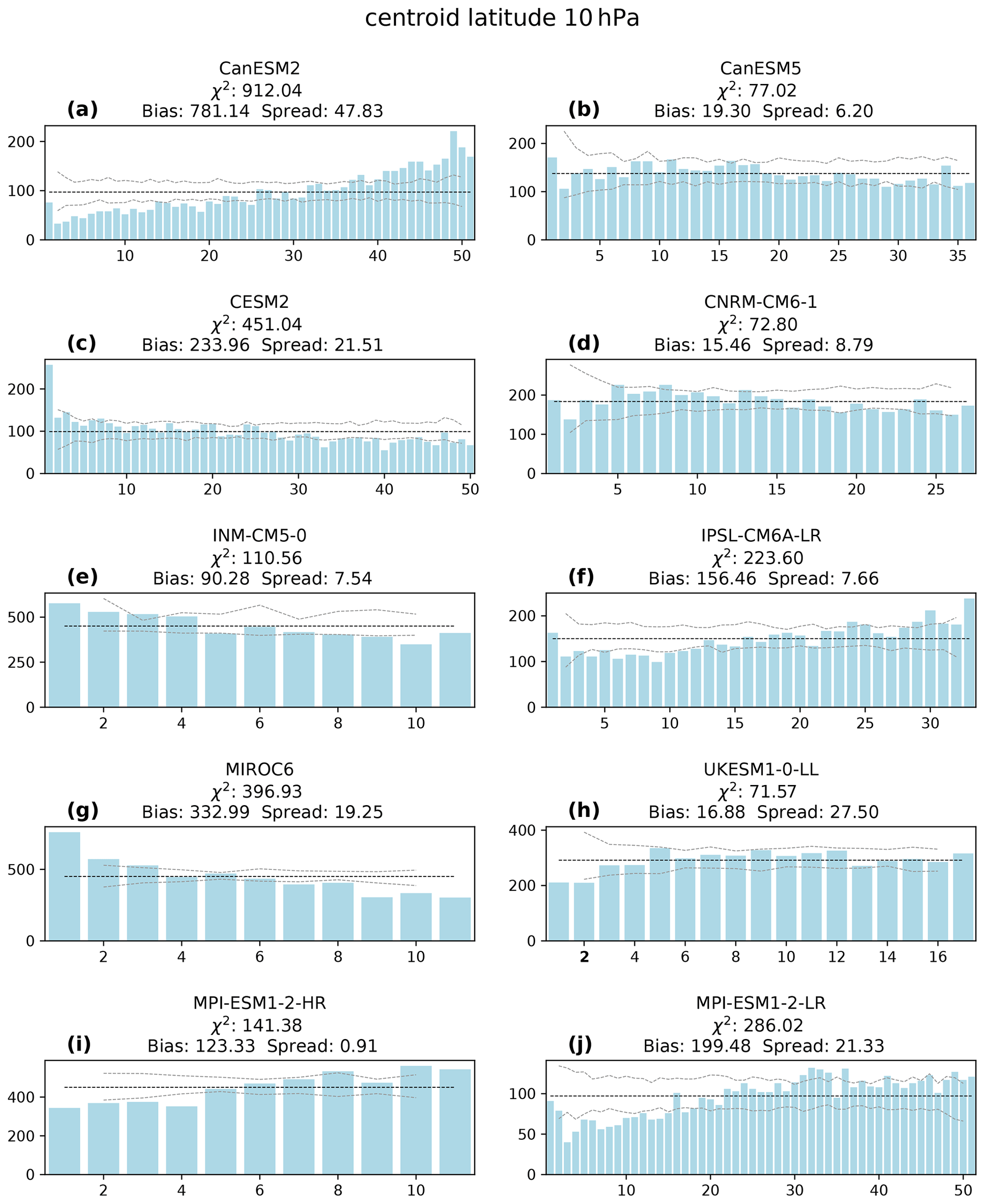
Figure 4 As Fig. 3 but for centroid latitude at 10 hPa for all analyzed model ensembles: CanESM2 (a), CanESM5 (b), CESM2 (c), CNRM-CM6-1 (d), INM-CM5-0 (e), IPSL-CM6A-LR (f), MIROC6 (g), UKESM1-0-LL (h), MPI-ESM1-2-HR (i) and MPI-ESM1-2-LR (j).

The RHs of the centroid latitude at the two lower-altitude levels are shown in Figs. S4 and S9. In most models, the bias is similar at all analyzed levels (10, 50 and 100 hPa), showing that the performance with respect to centroid latitude is not very sensitive to altitude. Only in CanESM5 does a low-latitude bias appear at the two lower altitudes. In MIROC6 the low-latitude bias is only present at 10 and 50 hPa, while at 100 hPa the model shows almost no bias and thus a nearly perfectly flat histogram.

3.3 Centroid longitude

The centroid longitude in the climate models ranges from −180 to +180°; the negative values lie in the Western Hemisphere and the positive ones in the Eastern Hemisphere. The centroid longitude RHs (Fig. 5) show where the climate models over- or underestimate the position of the SPV. When the counts are lower/greater than average, the ensemble simulates the SPV center more/less frequently at the respective longitude. The centroid longitude is depicted best by the CNRM-CM6-1 (see Fig. 5d) and INM-CM5-0 (see Fig. 5e) ensembles. The other ensembles show notable deviations from a flat histogram, but these deviations are not consistent among the models. The CanESM2, CESM2 and UKESM1-0-LL ensembles simulate the SPV center in the Eastern Hemisphere more frequently than the reanalysis. The IPSL-CM6A-LR and MIROC6 ensembles show the opposite bias. The RHs of CanESM5 (see Fig. 5b) and the MPI-ESMs (see Fig. 5i–j) show lower counts on both ends, indicating that the ensembles simulate the SPV more frequently in and around the region of the Bering Strait and Alaska (the meridian of +180/−180°) than the reanalysis.

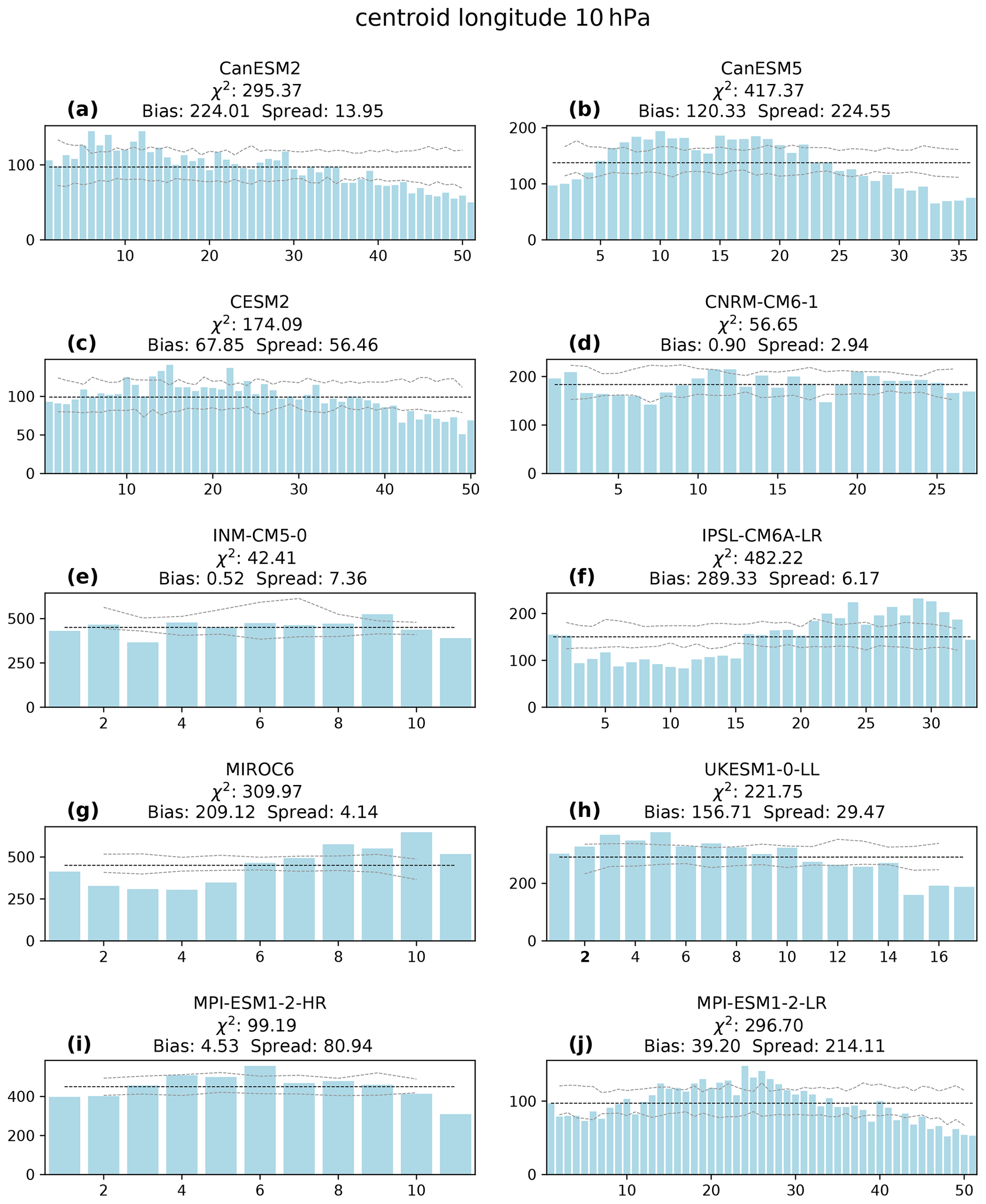
Figure 5 As Fig. 3 but for centroid longitude at 10 hPa for all analyzed model ensembles: CanESM2 (a), CanESM5 (b), CESM2 (c), CNRM-CM6-1 (d), INM-CM5-0 (e), IPSL-CM6A-LR (f), MIROC6 (g), UKESM1-0-LL (h), MPI-ESM1-2-HR (i) and MPI-ESM1-2-LR (j).

At 50 and 100 hPa (Figs. S5 and S10), some models show biases of opposite sign to that at 10 hPa, or even a general dispersion at the three different pressure levels (e.g., CanESM2, IPSL-CM6A-LR, MIROC6). This could not be seen for the centroid latitude. In most models, both bias and spread are present at least at some pressure levels. Only CNRM-CM6-1 produces a flat histogram where almost all counts lie inside the perfect model range in all three pressure levels. The UKESM1-0-LL and MPI-ESM1-2 ensembles show flat histograms at 50 and 100 hPa.

3.4 Kurtosis

The excess kurtosis is a measure for how the values of geopotential height are distributed within the SPV region (Matthewman et al., 2009). Mitchell et al. (2011) proposed that this diagnostic can be used to detect both SPV split and displacement events. They showed that exceptionally low values are often an indication that an SPV split has occurred. High positive values, on the other hand, can occur after splits and displacements (see their Figs. 2 and 5). The RHs for the excess kurtosis at 10 hPa are shown in Fig. 6. Four models show similar RHs with much higher counts on the left side of the histogram, namely CanESM2, CanESM5, CESM2 and CNRM-CM6-1. These ensembles underestimate the variability of the kurtosis and additionally simulate a kurtosis positive bias. The result is that very low values of the kurtosis are simulated much less frequently in the models than they occur in the reanalysis. Therefore, this may contribute to the underestimation of the SPV split frequency. This is in line with the aspect ratio low bias in these models (see Sect. 3.1), except for CNRM-CM6-1 (see Fig. 6d). Although the deviations are much less pronounced, the UKESM1-0-LL (see Fig. 6h) ensemble kurtosis shows similar behavior to the four model ensembles mentioned above with too few low values. This is in line with the results by Hall et al. (2021), who reported that the model simulates too few split events. The MIROC6 and INM-CM5-0 ensembles perform best in representing the kurtosis, in particular at 10 hPa. Both MPI-ESM1-2 simulations contain bias, but a dome-shaped RH in MPI-ESM1-2-LR indicates a large-ensemble spread.

Figure 6 As Fig. 3 but for kurtosis at 10 hPa for all analyzed model ensembles: CanESM2 (a), CanESM5 (b), CESM2 (c), CNRM-CM6-1 (d), INM-CM5-0 (e), IPSL-CM6A-LR (f), MIROC6 (g), UKESM1-0-LL (h), MPI-ESM1-2-HR (i) and MPI-ESM1-2-LR (j).

At the two lower altitudes (Figs. S6 and S11), most ensembles underestimate the kurtosis variability (CanESM2, CanESM5, CESM2, INM-CM5-0, UKESM1-0-LL and GFDL-CM3 at 100 hPa). Only the IPSL-CM6A-LR and both MPI-ESM1-2 ensembles overestimate it. The MPI-ESM1-2 ensembles show almost flat RHs at 100 hPa. Generally, most models simulate the kurtosis less well than centroid latitude or aspect ratio, in particular at 10 hPa. This suggests that lower-order moment diagnostics such as centroid latitude and aspect ratio are more reliable than kurtosis as a diagnostic combining fourth- and second-order moments (Matthewman et al., 2009).

3.5 Objective area

The objective area is of interest because a larger/smaller area of low geopotential height is often related to a stronger/weaker SPV with higher/lower wind speeds. Multiple ensembles (INM-CM5-0, IPSL-CM6A-LR, MIROC6, and both high- and low-resolution MPI-ESM1-2 ensembles) simulate a negative bias at 10 hPa (Fig. 7). In addition to that, these models underestimate the variability of the objective area. The CanESM2 (see Fig. 7a) ensemble also shows this combination but not as pronounced as the above-mentioned models. The CanESM5, CESM2 and CNRM-CM6-1 ensembles simulate a positive SPV area bias, which is likely connected to anomalously high wind speeds.

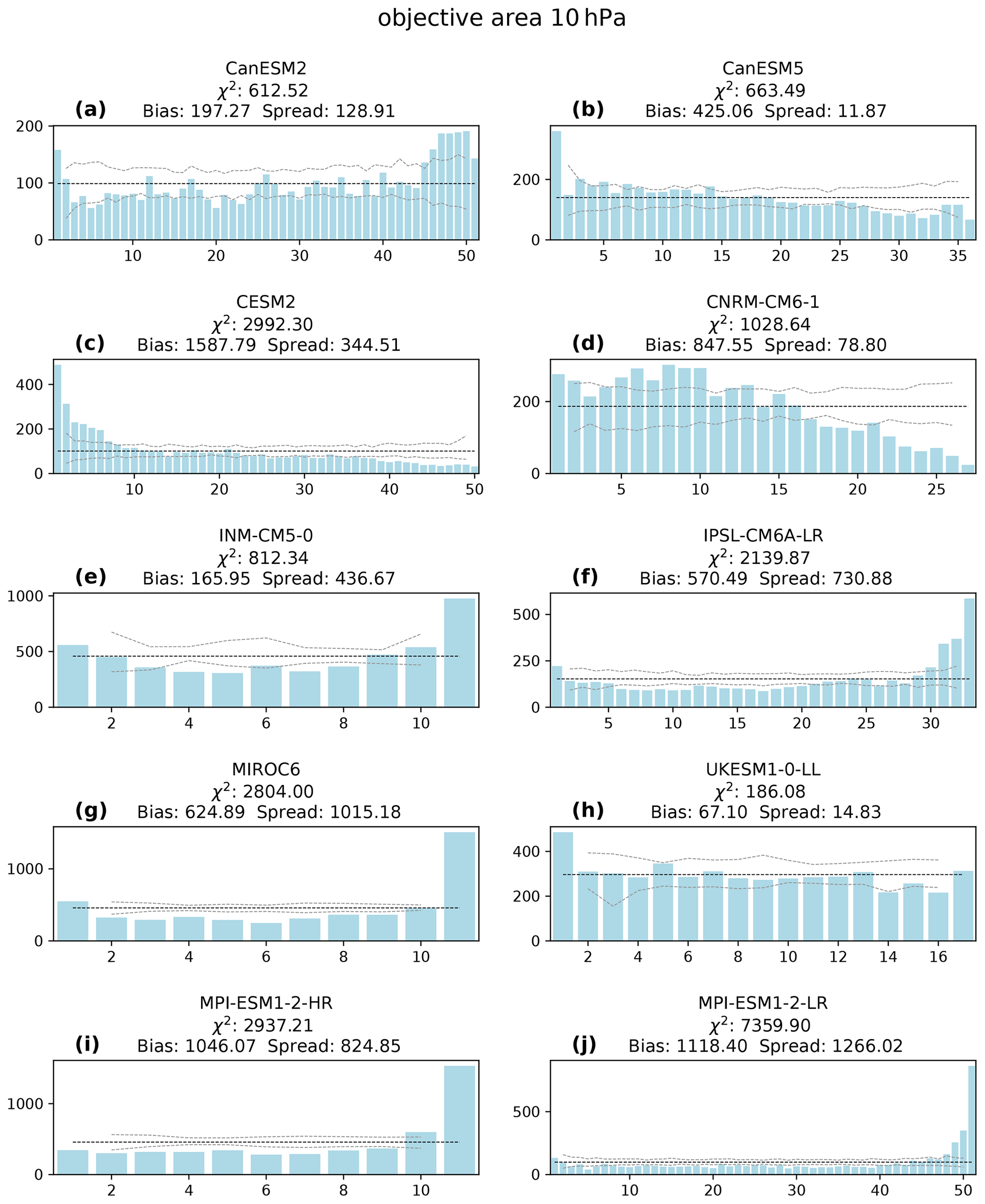
Figure 7 As Fig. 3 but for objective area at 10 hPa for all analyzed model ensembles: CanESM2 (a), CanESM5 (b), CESM2 (c), CNRM-CM6-1 (d), INM-CM5-0 (e), IPSL-CM6A-LR (f), MIROC6 (g), UKESM1-0-LL (h), MPI-ESM1-2-HR (i) and MPI-ESM1-2-LR (j).

At the lower altitudes (see Figs. S7 and S12) most models are biased in the same direction as at 10 hPa, but in some models the strength of the bias varies with height. Only INM-CM5-0 shows a weak SPV area bias at 10 hPa (see Fig. 7f) and a strong SPV area bias at 50 hPa. At 100 hPa barely any bias can be detected in INM-CM5-0. Models with a large SPV area bias at 100 hPa also simulate a low aspect ratio bias at 10 hPa (CanESM2, CanESM5, CESM2) and vice versa (IPSL-CM6A-LR and both MPI-ESM1-2 ensembles – except for MIROC6). Models without any notable bias (irrespective of the spread) for the objective area show a good representation of the aspect ratio (CNRM-CM6-1, INM-CM5-0, UKESM1-0-LL). A connection between weaker stratospheric winds and SPV split frequency in the CMIP6 models was already noted by Hall et al. (2021). They found that the frequency of SPV splits was related to the wind speeds at 100 hPa, because higher wind speeds hinder the upward propagation of wave number 2 planetary waves into the stratosphere. Similarly, Wu and Reichler (2020) showed that the highest uncertainty in the SSW frequency comes from uncertainty in lower stratospheric wind speeds. In general, most models do not simulate the objective SPV area well. Most commonly, they underestimate the variability and often simulate a bias. At 10 hPa the UKESM1-0-LL ensemble represents the SPV area best. At the two lower altitudes, CNRM-CM6-1 shows the best representation, depicted by the lowest values of the χ² statistic.

4 Sudden-stratospheric-warming analysis

A particular focus in NH SPV studies lies on disruptive SPV events, so-called sudden stratospheric warmings (SSWs). We here assess the ability of the climate models to distinguish between SSWs and steady SPV conditions. While the RHs reveal reliability (consistency), they do not evaluate statistical resolution (the degree to which a forecast sorts the observed events into different groups), so our study needs to be accompanied by other tools such as the ROC (Hamill, 2001). Using the ROC we can analyze how well the different models are able to simulate SSW events through diagnostics of the SPV morphology. The applied method allows us to individually diagnose displacement- and split-type SSWs. Hence, we conduct two separate analyses here, as it has been shown that these events, as well as their surface impact, fundamentally differ (Baldwin et al., 2021, and references therein).

4.1 Displacement events

Figure 8 shows the areas under the ROC curves (AUC) of the analyzed climate models for detection of SPV displacements (see Fig. 8a) and splits (see Fig. 8b). For all ROC curves see Figs. S1 and S2. We also summarize AUC values from these figures in Table S1.

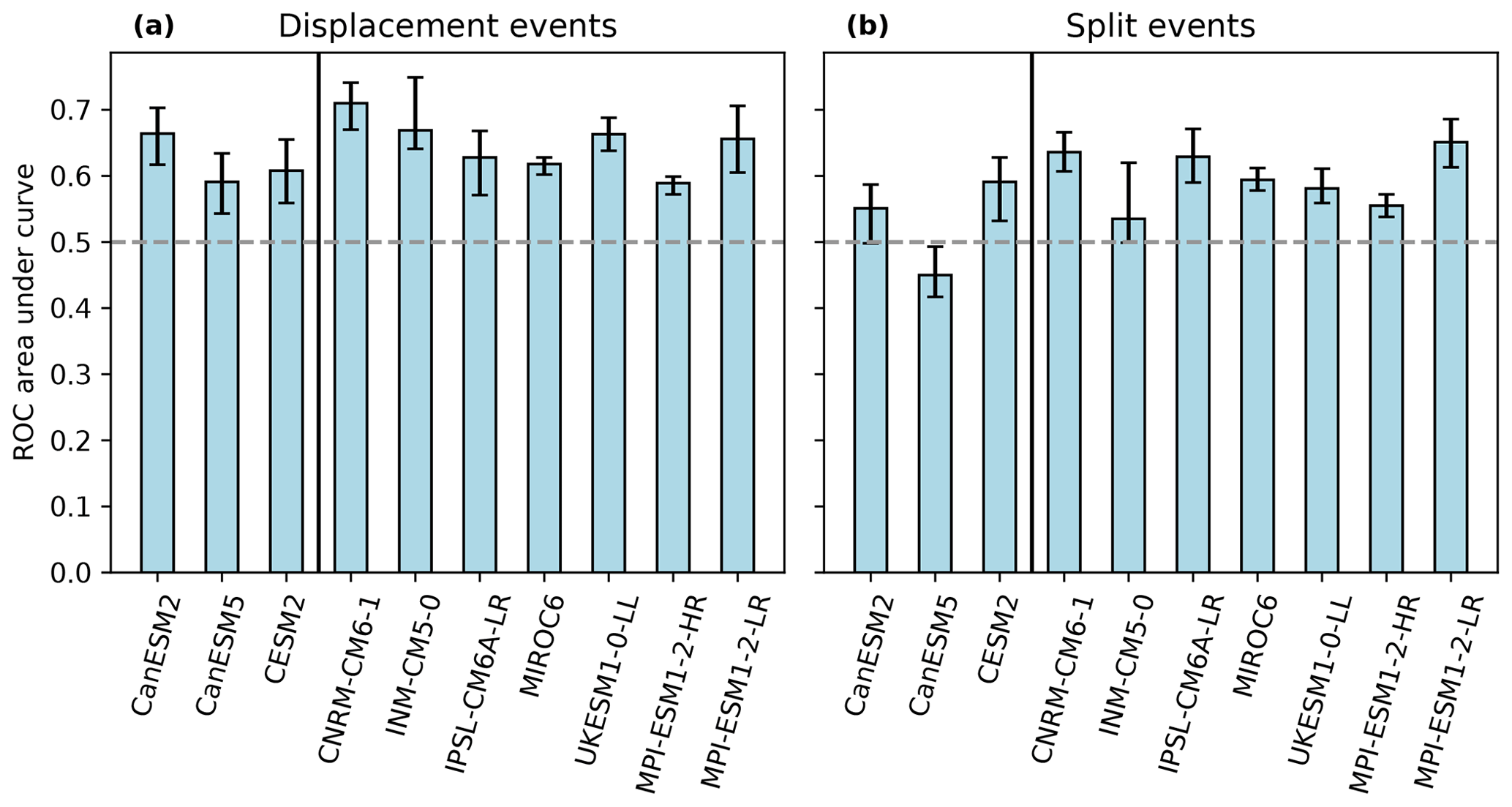
Figure 8 Area under the curve for the ROC curves of the analyzed climate ensembles for displacement (a) and split (b) events. The gray line lies at 0.5, the value at which the simulation is not better than randomly guessing. Low-top models are separated on the left with a black line. Error bars indicate 5th and 95th percentile estimated by using the perfect model range.

In general, the low-top models (see Table 1) reveal lower AUC values than the high-top models, with the exception of MPI-ESM1-2-HR. In fact, MPI-ESM1-2-HR has the lowest value of all analyzed models. Additionally, the AUC for the MPI-ESM1-2-HR ensemble is slightly lower than for its low-resolution counterpart MPI-ESM1-2-LR. The CNRM-CM6-1 ensemble shows the best performance regarding the simulation of SPV displacement events. This model also has one of the best representations of the centroid latitude at 10 hPa in the RHs. In fact, the RH was similar to CanESM5, for which a rather weak performance in the ROC curves was found. A reasonable performance is shown by the INM-CM5-0 ensemble, which in fact has the second-highest AUC. IPSL-CM6A-LR and MIROC6 show similar values for the AUC. The UKESM1-0-LL and MPI-ESM1-2-LR ensembles show an above-average performance compared to the other climate models. Again, this stands partly in contrast to the rank histograms where the UKESM1-0-LL ensemble was closest to a flat histogram of centroid latitude with the lowest χ² statistic of all models.

These results demonstrate that even if the RH implies a good representation, i.e., a reliable ensemble, it can show a comparatively low statistical resolution in distinguishing between displacements and non-displacements (e.g CanESM5) and vice versa (e.g., CESM2). Generally, for most of the ensembles, the AUC lies in a narrow region around 0.6, implying that the simulation of displacement events can still be improved in the climate ensembles, e.g., by calibration (Wilks, 2011).

It has been suggested by Seviour et al. (2016) and Hall et al. (2021) that models with a bias in centroid latitude also have a bias in displacement frequency in the respective direction. While we reproduce this negative relationship between number of displacements and modal centroid latitude from Fig. 3a in Hall et al. (2021) in our Fig. 9a, we observe models that despite their biases in modal centroid latitude simulate a comparable frequency of displacement SSWs. The CNRM-CM6-1 ensemble is again the best-performing one in terms of the frequency of displacement SSWs comparable to ERA5 (∼ 4 events per decade).

Figure 9 Scatter plots of modal centroid latitude [deg] and frequency of displacement SSWs (a), and modal aspect ratio and frequency of split SSWs (b) [per decade] in large ensembles compared with ERA5. Blue solid and dashed lines are ordinary least squares regressions and their 95 % confidence intervals for all models, while gray lines in panel (b) show regression lines and confidence intervals for high-top models only (i.e., except CESM2 and CanESM2). The dotted lines represent results for ERA5. Horizontal shading indicates the frequency of displacement or split events and represents the 1σ range, assuming a binomial distribution of events. Vertical shading was calculated using bootstrapping of ERA5 time series and represents the 1σ range. The error bars represent standard deviation through ensemble members shown as dots. $R_{\mathrm{adj}}^{\mathrm{2}}$ represents the adjusted coefficient of determination. The asterisks flag levels of significance with a p value less than 0.01.

4.2 Split events

In general, the climate model ensembles do not simulate SPV splits (see Fig. 8b) as well as SPV displacements (see Fig. 8a). Indeed, all models except for IPSL-CM6A-LR have lower AUCs for split events than for displacements. Overall, the weaker performance of the low-top models can be detected, which is particularly obvious for CanESM5. The ensemble performs worse than its older counterpart CanESM2 and shows a ROC area of below 0.5, which means that the false-positive rate for detecting split events is higher than the true-positive rate. In fact, CanESM5 is the only model that produces an AUC of lower than 0.5 for split events (see also Fig. 2), even when considering the error bars. Although the CESM2 ensemble shows a similarly strong aspect ratio bias as CanESM5, it has a better representation of split events according to the ROC plots.

As for displacement events, CNRM-CM6-1 also reaches one of the largest AUC for splits after MPI-ESM1-2-LR (see also Table S1). Thus, this model can be regarded as having the best representation of SPV displacements as well as splits and SSW events in general (see also Fig. 9). The AUC of the INM-CM5-0 ensemble reaches a value of slightly above 0.5, indicating that the simulation of splits is only marginally better than randomly guessing their occurrence. This result stands in contrast to the fact that this ensemble has shown one of the best performances in the RH analysis for the aspect ratio without any significant bias or spread. This again corresponds to the insensitivity of the ROC to certain biases as discussed above. The IPSL-CM6A-LR ensemble, on the other hand, almost reaches the performance of CNRM-CM6-1 in spite of its bias to predict higher aspect ratios too often. MIROC6 and UKESM1-0-LL show similar AUCs that lie between the best- and weakest-performing ensembles. The high-resolution MPI-ESM1-2 ensemble is showing a lower AUC than the low-resolution version MPI-ESM1-2-LR, as it was already seen for displacement events, but it still remains well above the value of 0.5.

In accordance with the results by Seviour et al. (2016) and Hall et al. (2021), we tried to reproduce whether models showing a strong bias to lower aspect ratios in our analysis indeed underestimate the SPV split frequency. However, results in Fig. 9b are more dispersed compared to Hall et al. (2021). It reveals that the linear relationship between number of splits and modal aspect ratio from Fig. 3b in Hall et al. (2021) cannot be reproduced in the large-ensemble simulations of the here used high-top models. It only works to some degree when low-top models are included. Unlike their results, the reanalysis values lie within the 95 % confidence interval of the ordinary least squares fit. As we can rule out that the size of ensemble members might not be sufficiently large in our study, we argue that the fit may not be so robust for split SSWs because a stretching tendency of the polar vortex is accompanied by a centroid latitude tendency to equatorward values (Mitchell et al., 2011). This finding also underlines our statement that good performance in representing the geometric-based diagnostics in RHs is not necessarily connected with a good performance in simulating displacements and splits. Wu and Reichler (2020) also demonstrated that bias-corrected models for vortex strength may not consistently align with reanalyses in terms of revealing SSW frequency.

5 Summary and discussion

We assessed the SPV in large CMIP5 and CMIP6 climate model ensembles using RHs with reference to ERA5 reanalysis data. The performance of the models varies depending on the analyzed variables and pressure levels. No model ensemble can be highlighted as having the best or worst performance over all variables and pressure levels. If the general performance over all levels and variables is regarded, the CNRM-CM6-1 and UKESM1-0-LL ensembles can be considered to be representing SPV form and variability best. These two models produce a flat RH for most of the geometric variables at most altitudes, which means that the simulated SPV in these models agrees well with that of ERA5. The flat RH is a necessary but not a sufficient condition for concluding reliability in SPV simulation.

Furthermore, we used the ROC analysis in order to assess the ability of the ensembles regarding SPV displacement and split frequencies. As all models reach an area under the ROC curve of more than 0.5 (see Fig. 8a), they distinguish between SPV displacements and non-displacements better than random guessing. In general, the ensembles represent displacement events better than split events. CNRM-CM6-1 has the best representation of both SPV splits and displacements. This model performs well in the RH analysis as well. However, a general rule of thumb that connects the RH with the ROC analyses could not be found here. This is due to the insensitivity of the ROC to biases in the forecast. The ROC diagram can be considered as a measure of potential usefulness when a model ensemble is correctly calibrated (Wilks, 2011). This can lead to a more reliable forecast while maintaining good discrimination. A joint analysis of variety diagnostics provides the bigger picture about the quality of large-ensemble model simulations.

Low-top models reveal strong biases for most variables, in particular CESM2. Charlton-Perez et al. (2013) and Hall et al. (2021) already found that low-top models simulate too few SSWs and too low variability of the SPV wind speeds. As stated in Wu and Reichler (2020), a finer vertical resolution also improves the simulation of SSW frequency. This means that the downward influence of the upper stratosphere and mesosphere has a large influence on the SPV and on SSWs (see, e.g., Hitchcock and Simpson, 2014). This is not unexpected, as large amounts of wave drag are deposited at high altitudes, which strongly influences middle atmosphere dynamics. In the low-top models, this influence is not adequately represented. Models with more vertical levels in the stratosphere generally perform better in our analysis. CNRM-CM6-1, which has the second-highest number of levels in the vertical, does not only have a good representation of most variables but also the best results in detecting splits and displacements. While the models with moderate spatial (vertical and horizontal) resolution (INM-CM5-0 and MIROC6) show a good performance, especially for the aspect ratio and kurtosis at 10 hPa, the MPI-ESM1-2-LR ensemble produces better results despite its vertical and horizontal resolution. Dedicated model experiments with simulations in various horizontal and vertical resolutions are needed to systematically assess the impact of resolution on SPV representation.

An additional source of uncertainty might be the gravity wave (GW) parameterizations (e.g., Eichinger et al., 2020; Karami et al., 2022; Eichinger et al., 2023). Events with strong gravity wave drag can affect the refractive index in the lower stratosphere (Kuchar et al., 2022). A higher refractive index results in stronger upward-propagating wave activity, and thus the SPV is disrupted more easily. Wu and Reichler (2020) found that the uncertainty of the refractive index in the lower stratosphere plays an important role for the uncertainty in SSW frequency, indicating that these uncertainties may be attributed to different GW parameterizations (Sigmond and Shepherd, 2014). Recently, Hájková and Šácha (2023) showed that the SPV climatologies are largely insensitive to high-latitude wave drag, but they also mentioned their sensitivity to nuances in model dynamics. Dedicated analyses are needed to fully assess the non-linear feedbacks of various wave drag mechanisms on SPV geometry and SSWs. For example, Sigmond et al. (2023) have attributed the difference in SSW frequency between CanESM2 and CanESM5 (especially splits as seen in Fig. 9b) to changes in GW settings.

Apart from model resolution and GW parameterizations and their tuning parameters, Morgenstern et al. (2022) revisited the influence of stratospheric ozone chemistry on the SPV and SSW frequency. Several additional studies demonstrated the importance of interactive ozone chemistry for representing temperature variability and extremes in the Arctic polar stratosphere (Haase and Matthes, 2019; Rieder et al., 2019; Oehrlein et al., 2020). Therefore, the way in which atmospheric chemistry is treated in the model may be another factor for model skill in representing the SPV, in particular the feedback of stratospheric ozone on dynamics via radiation. CNRM-CM6-1 has a simplified but still interactive chemistry (Voldoire et al., 2019). The only analyzed model with a complete interactive chemistry is UKESM1-0-LL, and overall it performs well. However, a detailed analysis of its impact on spatiotemporal SPV variability would be needed for conclusive statements.

Models that were found to simulate well the alternating easterlies and westerlies in the tropics by Richter et al. (2020) (the quasi-biennial oscillation, QBO) mostly perform better in our analysis (e.g., CNRM-CM6-1, IPSL-CM6A-LR, UKESM1-0-LL). On the other hand, models with poor QBO representation (CanESM2, CanESM5, CESM2) show a weaker performance in the RHs and the representation of splits and displacements. The SPV is influenced via teleconnection associated with the QBO, via the so-called Holton–Tan mechanism (HTM; Holton and Tan, 1980; Baldwin et al., 2001). Rao et al. (2020) analyzed which models have a good representation of the HTM, but here we find no clear connection between a good HTM representation and a good representation of SPV variability.

While a relatively long period was regarded in the RH analysis, it cannot be ruled out that an ensemble might show different performances during this time (Bothe et al., 2013). An option could be to analyze individual months separately since differences in the model performance might, for example, occur between mid-winter, where the highest variability in wind speeds is observed, and early as well as late winter.

Furthermore, the thresholds used for the definition of the events could be varied. Other values might lead to better resolution between steady and unsteady SPV conditions. The thresholds we used here were chosen based on the reanalysis dataset by Seviour et al. (2013) as stated in Sect. 2.5. Another important question is whether the number of ensemble members is sufficient for evaluation of the highly variable SPV representation. In particular, the INM-CM5-0, MIROC6 and MPI-ESM1-2-HR ensembles may not be large enough to fully cover the effective dimension of SPV (Christiansen, 2021). This is a topic for detailed future investigation.

6 Conclusions

In this study, we assess the stratospheric polar vortex (SPV) morphology and its variability in large CMIP5 and CMIP6 climate model ensembles. Moreover, we analyze the ability of the models to distinguish different types of sudden stratospheric warmings (SSWs), i.e., splits and displacements, and use ERA5 reanalysis data as a reference. These analyses reveal strongly varying performances of the individual models over all SPV moment diagnostics and pressure levels. The two models that overall simulate the SPV and SSWs closest to ERA5 are CNRM-CM6-1 and UKESM1-0-LL. In contrast, the results of CanESM5 and CESM2 should be handled with particular care in SPV studies, as these models did not perform well in our analysis. In general, the ensembles show a better ability in simulating displacement-type SSW events than split-type events. As SSWs represent extreme events, this model skill, however, is not always connected with representing well the geometry-based SPV morphology diagnostics, which diagnose SPV climatologies.

For the latitude of the SPV center (centroid latitude) and the stretching parameter (aspect ratio), most ensembles are biased to some extent but with no consistent direction among the ensembles. While regression of these geometric SPV biases indicates also biases in split and displacement frequency as in Seviour et al. (2016) and Hall et al. (2021), this does not necessarily imply that bias-corrected models simulate split and displacement frequencies according to the reanalyses (Wu and Reichler, 2020). Out of all analyzed diagnostics, the SPV splitting diagnostic excess kurtosis (Matthewman et al., 2009) appears to be the hardest one to simulate correctly. Most of the ensembles underestimate the variability of the kurtosis. Strong biases and an underestimation of the variability is also found for the SPV area, which is a measure for SPV strength. Overall, this may be constituted by the difficulty of models to simulate the well-known non-linearity of stratospheric dynamics (Matthewman and Esler, 2011; Cohen et al., 2014; Eichinger et al., 2020) and calls for caution when using these diagnostics as SSW proxies.

We conclude that usually models with a higher lid and models with a finer vertical resolution generally simulate the SPV and SSWs better with reference to ERA5. However, many factors influence SPV properties and SSW frequency, such as interactive chemistry, gravity wave parameterizations and other dynamical processes that differ in the individual models. It is therefore not possible to clearly determine from this study which model characteristics are the decisive ones for representing the SPV and its variability well.

Knowledge of how well different climate models perform in simulating the SPV spatial variability and SSWs correctly is of utmost importance for tuning and calibrating to improve their performance, as well as for assessing their reliability in future climate projections. The latter is particularly important with regard to polar stratospheric ozone and its evolution across the 21st century.