the Creative Commons Attribution 4.0 License.
the Creative Commons Attribution 4.0 License.
 | 31 Jul 2024
Circulation responses to surface heating and implications for polar amplification
Peter Yu Feng Siew
Camille Li
Stefan Pieter Sobolowski
Etienne Dunn-Sigouin
Mingfang Ting
A seminal study by Hoskins and Karoly (1981) explored the atmospheric circulation response to tropospheric heating perturbations at low latitudes and midlatitudes. Here we revisit and extend their study by investigating the circulation and temperature response to low, middle, and high latitude surface heating using an idealised moist grey radiation model. Our results corroborate previous findings showing that heating perturbations at low latitudes and midlatitudes are balanced by different time-mean circulation responses – upward motion and horizontal-temperature advection, respectively. Transient eddy heat flux divergence plays an increasingly important role with latitude, becoming the main circulation response at high latitudes. However, this mechanism is less efficient at balancing heating perturbations than temperature advection, leading to greater reliance on an additional contribution from radiative cooling. These dynamical and radiative adjustments promote stronger lower-tropospheric warming in response to surface heating at high latitudes compared to lower latitudes. This elucidates the mechanisms by which sea ice loss contributes to polar amplification in a warming climate.
- Article
(2958 KB) - Full-text XML
-
Supplement
(3009 KB) - BibTeX
- EndNote


There is strong consensus that the Arctic has warmed at a rate more than twice the global average over recent decades (e.g. Serreze et al., 2009; Cohen et al., 2014; Previdi et al., 2021; England et al., 2021; Rantanen et al., 2022). Concurrent with this warming, there has been a rapid decline in sea ice that acts as both a response and a contributor to the Arctic amplification signal (Cohen et al., 2014; Dai et al., 2019; Olonscheck et al., 2019). The shrinking sea ice cover exposes relatively warm ocean waters that warm the lower troposphere through turbulent exchanges. It is hypothesised that this additional energy input at the surface can modify the large-scale circulation through several proposed mechanisms (see Cohen et al., 2020; Outten et al., 2023). However, detecting such linkages and identifying robust physical mechanisms pose challenges (e.g. Sellevold et al., 2016; Shepherd, 2016; Mori et al., 2019; Siew et al., 2020, 2021; Labe et al., 2020; Sun et al., 2022; Shaw and Smith, 2022; Zheng et al., 2023), in large part because our dynamical understanding of Arctic-midlatitude teleconnections remains incomplete (Wallace et al., 2014; Hoskins and Woollings, 2015; Woollings et al., 2023).
There is a rich history of investigations aimed at improving fundamental understanding of the atmospheric response to heating perturbations. A paradigmatic demonstration of differences in how the atmosphere adjusts to heating in the tropics versus the midlatitudes was presented by Hoskins and Karoly (1981). Using a linearised five-layer baroclinic model, Hoskins and Karoly (1981) showed that the circulation response to heating attempts to offset or balance the perturbation in the most efficient way possible. In the tropics, near-surface atmospheric heating induces deep tropospheric warming, and the resulting upward motion produces adiabatic cooling to balance the extra energy input. Conversely, in the midlatitudes, vertical motion is inhibited and near-surface heating is mainly balanced by horizontal temperature advection. In the lower troposphere, meridional advection is induced by a low-pressure anomaly downstream of the heating, which brings cold air from the pole; zonal advection plays an important role in the free troposphere, where zonal winds are stronger. Apart from these local responses, the surface heating, especially in the tropics, can excite large-scale Rossby waves that redistribute the energy input associated with anomalous heating. Similar dynamical responses to tropical and midlatitude surface heating have also been found in more comprehensive models and setups (Ting and Held, 1990; Ting, 1991; Hall et al., 2001; Walter et al., 2001; Inatsu et al., 2002, 2003; Deser et al., 2007).
Given the tropospheric heating associated with Arctic amplification of global warming and the fact that the circulation response to said heating is ambiguous, it is natural to extend the study of heating perturbations to high latitudes. At high latitudes, the high static stability, weak zonal wind, and weak meridional temperature gradient limit the ability of vertical and horizontal temperature advection to balance heating perturbations by the aforementioned atmospheric processes (Woollings et al., 2023). Additional processes such as radiative cooling have been hypothesised to be important in the polar regions (Kim et al., 2021; Woollings et al., 2023; Miyawaki et al., 2023), but the full adjustment mechanism has not been systematically explored. Such an investigation also offers an opportunity to revisit and extend the tropical and midlatitude heating results from Hoskins and Karoly (1981) using a grey radiation aquaplanet model that has no clouds or ice (Frierson et al., 2006). This modelling framework is still idealised but allows us to include some effects of moisture, surface energy fluxes and radiation that are hypothesised to help set the temperature and circulation responses to high-latitude heating (e.g. Winton, 2006; Langen et al., 2012; Kim and Kim, 2017; Matthews et al., 2022).
In this study, we carry out perturbation experiments by imposing surface heating from low (15° N) to high (75° N) latitudes in a zonally symmetric climate. The aforementioned idealised framework is well suited to isolating the fundamental physical processes that drive the atmospheric response to prescribed heating perturbations. We examine the physical links between atmospheric circulation and temperature responses to the heating perturbations, focusing on the differences between the polar heating experiments and heating at other latitudes.
2.1 Model setup and control experiment
We employed the idealised moist general circulation model documented in Frierson et al. (2006), Frierson (2007), and O'Gorman and Schneider (2008). The model was run using the Isca idealised modelling framework (Vallis et al., 2018), which allows one to easily modify the complexity of the various components in the model. In our setup, the model was integrated at T85 spectral resolution in the horizontal direction (1.4°×1.4° grid size) with 30 unevenly spaced sigma levels, from the surface to 3 Pa, in the vertical direction.
The model consists of a primitive equation atmosphere coupled to a slab ocean. The slab ocean does not include sea ice or the effects of changes in ocean circulation. Water is allowed to evaporate from the ocean to form water vapour, which is advected with the atmospheric flow. Moisture interacts with the atmospheric dynamics via the release of latent heat during condensation. All condensed water is precipitated immediately; hence, there are no clouds in the model. Additionally, the model uses a grey radiation scheme, where a single optical thickness is used across the entire longwave frequency band, meaning that radiative water vapour feedback is not represented. The longwave and shortwave optical thicknesses are prescribed as a function of latitude and altitude.
The control experiment follows the protocol of the Tropical Rain belts with an Annual Cycle and a Continent Model Intercomparison Project (TRACMIP), which has been used for aquaplanet setups in previous modelling studies (e.g. Voigt et al., 2016; Dunn-Sigouin et al., 2021). The protocol includes insolation forcing with present-day diurnal and seasonal cycles and a 30-metre slab ocean with a time-independent and zonally symmetric ocean heat flux convergence (Q-flux) that mimics the observed Equator-to-pole ocean heat transport (see Eq. 3 in Voigt et al., 2016). All other parameters not specified in the TRACMIP protocol were set following O'Gorman and Schneider (2008). The model was spun up for 20 years and then run for an additional 30 years to produce the control experiment. The zonal-mean zonal wind, air temperature, and transient eddy kinetic energy of the control experiment are shown in Fig. S1 in the Supplement. The temperature and wind show reasonable agreement with observations, although the eddies in the upper troposphere appear to be weaker in the model. In the control simulation, the weaker eddies may stem from the absence of sea ice in the model (Miyawaki et al., 2023). However, our findings remain consistent across the winter and summer seasons, which respectively exhibit stronger and weaker eddies compared to the annual mean, suggesting that our results are not sensitive to eddy strength in the control simulation.
2.2 Perturbation experiments
Experiments with imposed time-independent Q-flux perturbations representing localised heating anomalies were branched off from the control experiment. Each perturbation experiment was run for 30 years after discarding a 10-year spin-up. The system reaches equilibrium around the middle of this spin-up period, evident from the stabilisation of global mean surface temperature (Fig. S2). The form of the Q-flux perturbation follows the paraboloid function in Thomson and Vallis (2018):
and all negative values (i.e. outside of the paraboloid) are set to zero. The Q-flux perturbation has a maximum magnitude of Qmax at the central latitude and longitude of ϕo and λo, respectively. ϕd and λd describe the tapering of the Q-flux perturbation away from the maximum. We have five Q-flux perturbation experiments, with ϕo=15, 30, 45, 60, and 75° N spanning λd=32, 36, 44, 62, and 120° of longitude, respectively. For all experiments, we set the heating perturbation at λo=0° spanning ϕd=30° of latitude, and set Qmax=100 W m−2 (see Fig. 1). By design, all Q-flux perturbations are identical in areal extent and input the same amount of total energy into the system (about 450 TW). The response of a variable to the Q-flux perturbation is obtained by subtracting the annual-mean climatology of the control run from the perturbation experiment (i.e. perturbation minus control).
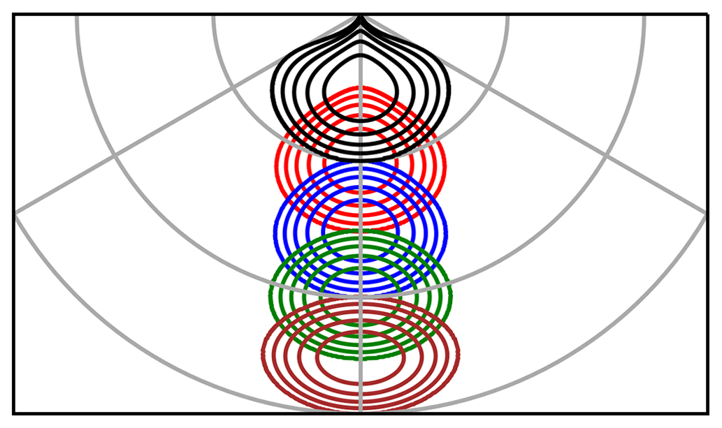
Figure 1Prescribed Q-flux in the heating perturbation experiments with heating at 15° N (brown), 30° N (green), 45° N (blue), 60° N (red), and 75° N (black). The latitude lines mark 0, 30, and 60° N. The longitude lines mark 60° W, 0, and 60° E. Contour intervals are 0, 20, 40, 60, and 80 W m−2. All Q-flux perturbations are identical in areal extent and input the same amount of total energy into the system (about 450 TW).
2.3 Thermodynamic equation
Following the framework from Hoskins and Karoly (1981), we use the steady-state thermodynamic equation to diagnose which heat transport terms balance the diabatic heating generated by the surface Q-flux perturbation. We extend the linearised quasi-geostrophic form of the steady-state thermodynamic equation used in Hoskins and Karoly (1981) to the full thermodynamic equation that includes transient eddy heat fluxes (Eq. 3.21 in James, 1995):
where u, v, and ω are the zonal, meridional, and vertical velocity, respectively; are the gradients of potential temperature in the zonal, meridional, and vertical directions, respectively; p is pressure and po is the reference pressure (=1000 hPa); R (=287 J kg−1 K−1) is the gas constant of air; and Cp (=1004 J kg−1 K−1) is the specific heat capacity of air at a constant pressure. The bars represent the time mean and primes represent the deviation from the time mean. The first three terms on the left side of Eq. (2) are the time-mean advection of potential temperature in the zonal, meridional, and vertical directions. The sum of the last three terms on the left side is the transient eddy heat flux divergence. On the right side, Q is the diabatic heating rate. The calculated from Eq. (2) as a residual of the transport terms on the left side is compared to the diabatic heating calculated from source terms in a column-integrated sense, and they yield very similar results (Fig. S3). This confirms that the residual method provides a good estimate of the diabatic heating.
2.4 Moist static energy budget
The thermodynamic equation (Eq. 2) quantifies the contributions of various transport terms (circulation processes) for balancing the diabatic heating added by the Q-flux perturbation. To bring in the relative importance of radiative processes, we consider the steady-state column-integrated moist static energy budget (similar to Eq. 13.47 in Peixoto and Oort, 1992):
where Fsurface describes the surface turbulent (sensible and latent) and radiative fluxes, Ftop describes the top-of-the-atmosphere radiative fluxes, u describes the zonal and meridional winds, and E describes the moist static energy. The last term (, where g=9.8 m s−2) describes the divergence of the vertical integral of moist static energy and is treated as residual of the first and second terms. Note that the transport term here represents the total transport (both time-mean and transient terms) of the moist static energy (the sensible, latent, and geopotential energy) in a column-integrated sense, which is different from the transport of potential temperature decomposed into time-mean and transient terms level by level on the left side of Eq. (2).
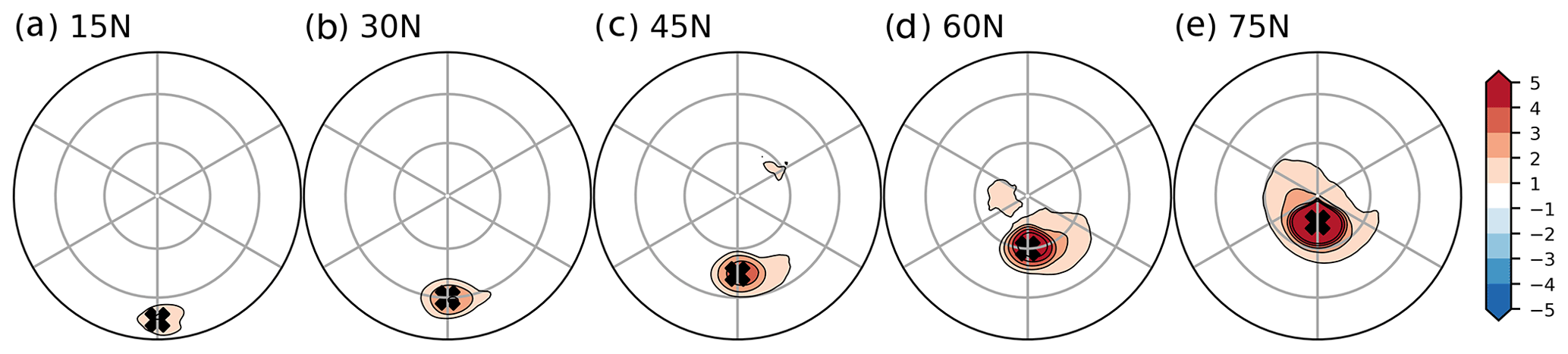
Figure 2Surface temperature response (K) in the (a) 15° N, (b) 30° N, (c) 45° N, (d) 60° N, and (e) 75° N heating perturbation experiments. The crosses mark the positions of the surface heating perturbations. The latitude lines mark 30 and 60° N. The longitude lines denote 60° intervals, marking 120° W, 60° W, 0°, 60° E, 120° E, and 180°.
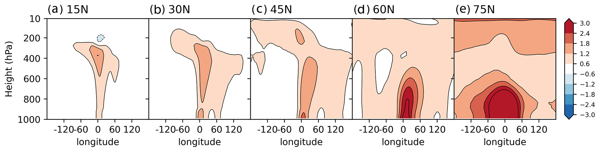
Figure 3Air temperature response (K) in the (a) 15° N, (b) 30° N, (c) 45° N, (d) 60° N, and (e) 75° N heating perturbation experiments. The longitude–height section shown is a meridional average over ±30° of latitude from the central latitude of the heating perturbations.
3.1 Temperature responses to heating perturbations from low to high latitudes
In this section, we explore the atmospheric response to surface heating from low to high latitudes via the previously described imposed Q-flux perturbation. The first-order response to surface heating is increased temperature at the surface (Fig. 2) and throughout the troposphere (Fig. 3) collocated with the heating sources. As the heating is moved from 15 to 75° N, the surface warming increases in magnitude (Fig. 2), and the maximum warming shifts from the upper to the lower troposphere (Fig. 3). The additional stratospheric warming for the 75° N heating experiment is consistent with an eddy-driven adjustment involving anomalous subsidence (see Hell et al., 2020). This response, while important, is not the focus of the present study. The amplified temperature response in the polar heating experiment resembles the Arctic amplification signal observed over the past few decades, whereby the Arctic has warmed faster than other parts of the globe, especially near the surface and in regions of rapid sea ice loss (Cohen et al., 2020; England et al., 2021; Rantanen et al., 2022).
We will first employ the idealised framework established in Hoskins and Karoly (1981) to explore what circulation responses balance the diabatic heating across the heating perturbation experiments (Sect. 3.2 and 3.3). Given that radiative processes are also important, we next quantify the relative importance of the circulation and radiative processes in balancing the energy input from the heating perturbations (Sect. 3.4). We start with heating perturbations centred at low latitudes and midlatitudes (15, 30, and 45° N), which yield results consistent with the near-surface heating experiments in Hoskins and Karoly (1981). Using these experiments as a baseline, we then move the heating perturbation towards higher latitudes (60 and 75° N), highlighting differences in the responses that can help clarify the physical link between real-world sea ice loss and Arctic amplification of global warming.
3.2 Mean low-level circulation responses to heating perturbations
Low-latitude to midlatitude surface heating generates vertical and meridional circulation responses in the lower troposphere that help balance the heating perturbation, consistent with Hoskins and Karoly (1981). The near-surface circulation response to the 15, 30, and 45° N surface heating shows vertical ascent (Fig. 4) and low pressure near the heating source (Fig. 5). The upward motion, which acts to balance the surface heating via adiabatic cooling, is particularly strong for the lowest-latitude (15° N) heating perturbation. Figure S4 further shows that the vertical ascent is accompanied by strong upper-level divergence over the heating source that further moves heat away from the atmospheric column. As the heating moves from 15 to 45° N, the anomalous upward motion becomes weaker, and the low-pressure centre shifts slightly eastwards, moving downstream of the heating source. This configuration tends to induce equatorward flow in the lower troposphere over the perturbation region and advect cold polar air to balance the heating (Hoskins and Karoly, 1981). Apart from these local circulation responses, we also find remote stationary wave responses (which exhibit clear zonal asymmetry) at both lower (Fig. 5) and upper levels (Fig. S5). The remote wave responses to heating at lower latitudes bear some similarities to those shown in Hoskins and Karoly (1981) but are not the focus of this study.
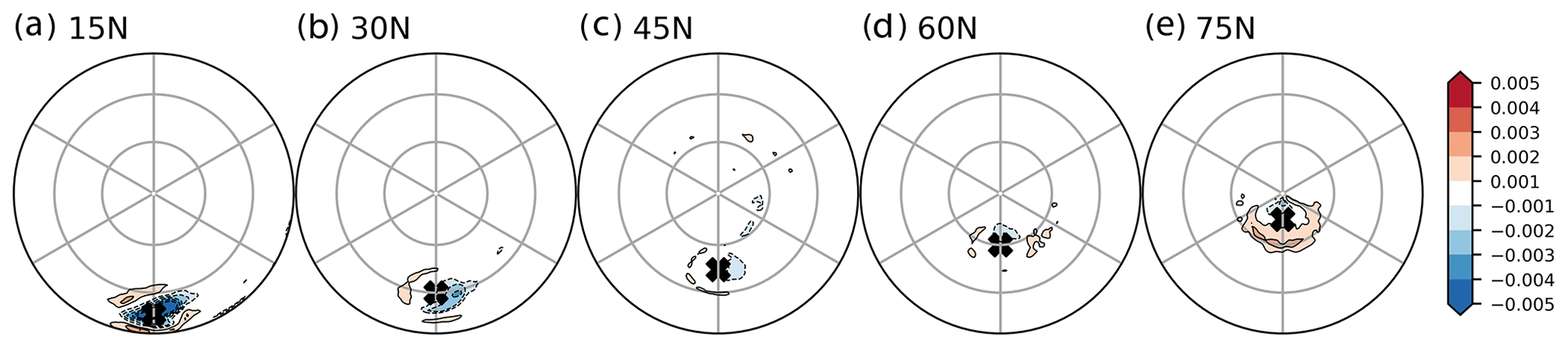
Figure 4Near-surface (990 hPa) vertical velocity response (Pa s−1) in the (a) 15° N, (b) 30° N, (c) 45° N, (d) 60° N, and (e) 75° N heating experiments. The crosses mark the position, of the surface heating perturbation,. The latitude lines mark 30 and 60° N. The longitude lines denote 60° intervals, marking 120° W, 60° W, 0°, 60° E, 120° E, and 180°.
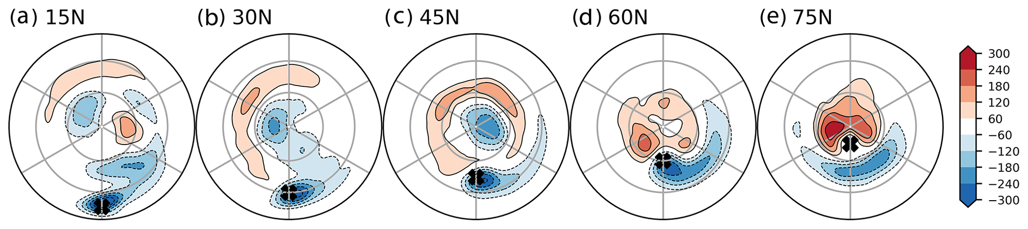
Figure 5Surface pressure response (Pa) in the (a) 15° N, (b) 30° N, (c) 45° N, (e) 60° N, and (e) 75° N heating experiments. The crosses mark the position, of the surface heating perturbation,. The latitude lines mark 30 and 60° N. The longitude lines denote 60° intervals, marking 120° W, 60° W, 0°, 60° E, 120° E, and 180°.
When the surface heating is placed further north at 60 and 75° N, there is less indication that mean circulation responses in the lower troposphere work to offset the extra heat. Near-surface upward motion (adiabatic cooling) is very weak for both high-latitude heating experiments, and there is even subsidence (adiabatic warming) to the south of the perturbation in the case of the 75° N experiment (Fig. 4e). The low-pressure anomaly still provides some cold-air advection to balance the 60° N heating source (Fig. 5d), as in the case of the midlatitude heating experiments. However, the low shifts equatorward in the 75° N experiment (Fig. 5e), and at the location of the heating source it is mostly offset by a zonally symmetric positive anomaly at the pole, reflecting a negative Arctic Oscillation (AO) or Northern Annular Mode (NAM) response that is commonly found in idealised polar heating (Butler et al., 2010; Wu and Smith, 2016; Zhang et al., 2018; Hell et al., 2020) and sea ice reduction (e.g. Magnusdottir et al., 2004; Deser et al., 2004, 2007, 2010) experiments. Removing the zonal-mean response to isolate the stationary wave pattern, we find a surface low nearly collocated with the 75° N heating source (not shown; consistent with Sellevold et al., 2016). Overall, mean meridional and vertical advection does not appear to play an important role in balancing high-latitude near-surface heating perturbations, as will be confirmed in Sect. 3.3.
3.3 Role of transient eddy fluxes versus mean circulation in balancing heating perturbations
The previous section qualitatively shows how the circulation responds to near-surface heating perturbations. Next, we quantify the relative importance of the circulation processes that balance the heating according to the thermodynamic equation (Eq. 2), namely, the time-mean zonal, meridional, and vertical potential temperature advection, as well as the transient eddy flux divergence. Figure 6 shows these terms in height–longitude sections near the heating source for each experiment (as differences between the perturbation and control). The first row shows the diabatic-heating term (right side of Eq. 2). The next three rows show temperature advection by the time-mean vertical, zonal, and meridional flow. The last row shows the transient eddy heat flux divergence. The sum of the heat transport terms (second to fifth row) equals the diabatic heating (first row). As described in Sect. 2.3, a direct calculation of column-integrated diabatic heating agrees well with the residual calculation shown here.
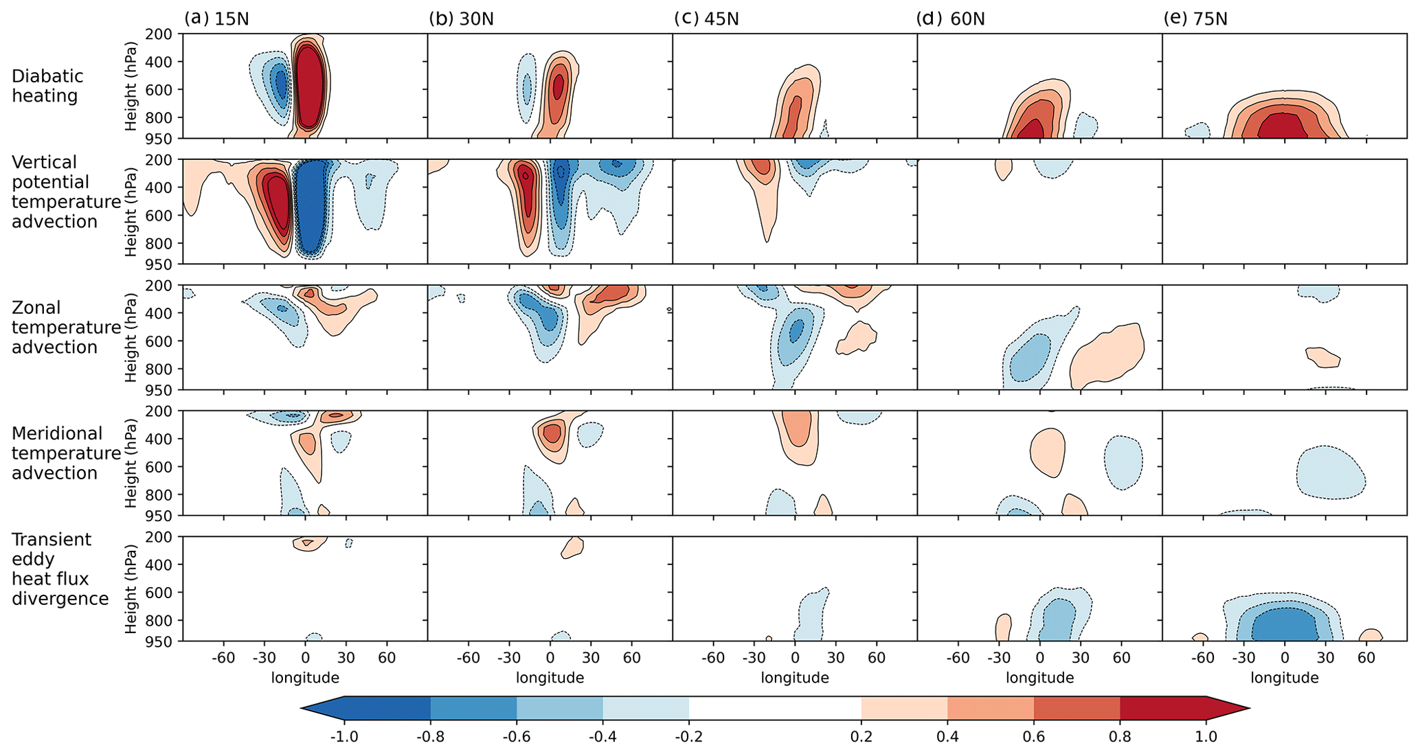
Figure 6The diabatic heating and heat transport terms (K d−1) in the (a) 15° N, (b) 30° N, (c) 45° N, (d) 60° N, and (e) 75° N heating experiments. The first row shows the diabatic heating, the second row shows the time-mean vertical potential temperature advection, the third row shows the time-mean zonal temperature advection, the fourth row shows the time-mean meridional temperature advection, and the fifth row shows the divergence of transient eddy heat fluxes. The longitude–height section shown is a meridional average over ±30° of latitude from the central latitude of the heating perturbations. All transport terms (second to fifth rows) are multiplied by −1 (i.e. moved to the right-hand side of Eq. 2) to highlight that they act to balance the diabatic heating.
Low-latitude (15 and 30° N) heating perturbations create deep diabatic-heating signals that maximise in the middle and upper troposphere (Fig. 6a and b), along with weak cooling upstream of the heating maximum. Consistent with the diagnostics in the previous section, such heating is in large part balanced by upward motion and hence adiabatic cooling over the heating maximum, while the weak cooling upstream is balanced by reduced convection and hence adiabatic warming. Note that in both the 15 and 30° N heating experiments, the horizontal temperature advection terms play some role in the lower troposphere, while the role of transient eddy heat flux divergence is still negligible.
The 45° N heating perturbation generates a shallower diabatic heating profile that maximises in the low-to-middle troposphere (Fig. 6c). As discussed in the previous subsection, the downstream low-pressure anomaly induces northerly flow that brings cold polar air from the north towards the western portion of the perturbation region in the lower troposphere; the middle to upper tropospheric signal is of the opposite sign, however. In the middle troposphere, zonal temperature advection also appears to play an important role in balancing the heating by advecting warm air sitting over the perturbation region further downstream, consistent with Hoskins and Karoly (1981). Apart from the time-mean horizontal advection, transient eddy heat flux divergence also moves excess heat out of the region in the low to middle troposphere, with magnitudes comparable to the meridional temperature advection near the surface. Note that the role of vertical advection is negligible throughout most of the troposphere in this experiment.
The heating perturbations at higher latitudes (60 and 75° N) create diabatic heating profiles that are concentrated in the lower troposphere (Fig. 6d and e). While the time-mean horizontal temperature advection still plays a role in balancing the 60° N heating in the middle and lower troposphere, the transient eddy heat flux divergence becomes as important at lower levels (Fig. 6d, fifth row). For the 75° N experiment, the transient eddy heat flux divergence is the dominant response (Fig. 6e).
Figure 7 summarises the results in this section by comparing the ratios of each circulation term to the total diabatic heating. The upper panel (Fig. 7a) considers the main regions covered by the heating sources (averaging over ±20° of longitude and latitude from the heating maximum) and the full troposphere (integrating from the surface to 200 hPa), with positive ratios indicating that the term acts to offset the perturbation. Moving from low to high latitudes, the time-mean vertical potential temperature advection becomes less important (blue bars; from 117 % to −13 %), while transient eddy heat flux divergence becomes more important (green bars; from 5 % to 86 %) in balancing the heating. The time-mean horizontal advection (red bars) appears to play a minimal role due to large cancellations between the zonal (yellow bars) and meridional (orange bars) components. Furthermore, in the whole-troposphere picture, the meridional advection is mostly negative due to its warming effect in the free troposphere (Fig. 6, fourth row). Considering only the lower troposphere (surface to 800 hPa) and the western portion (−20 to 0° longitude) of the heating perturbation highlights the importance of the horizontal temperature advection (red bars in Fig. 7b), especially for the midlatitude heating (30, 45, and 60° N experiments). In particular, the meridional advection (orange bars in Fig. 7b) is important for balancing the 30 and 45° N heating in the lower troposphere.
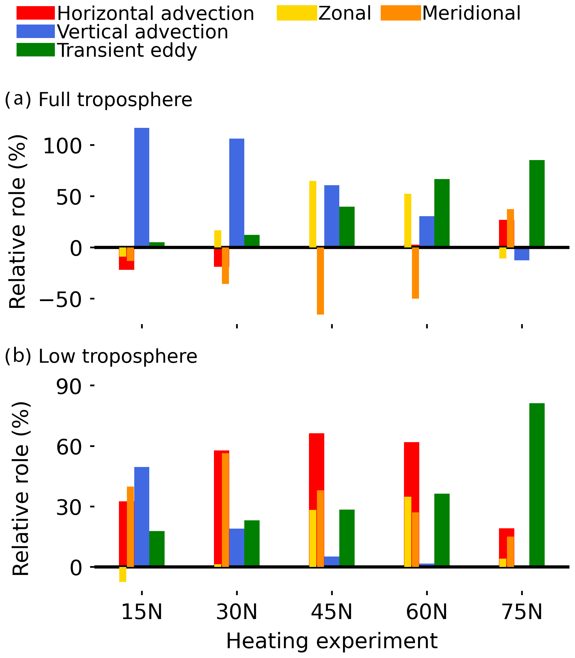
Figure 7Summary of the relative roles of the time-mean horizontal temperature advection (red), time-mean vertical potential temperature advection (blue), and transient eddy heat flux divergence (green) in balancing the diabatic heating. The time-mean horizontal temperature advection can be further decomposed into zonal (yellow) and meridional (orange) components. The relative role is the ratio between each heat transport term and the diabatic-heating term averaged within (a) ±20° of longitude and latitude from the heating maximum and integrated from the surface to 200 hPa and (b) −20 to 0° longitude and ±20° of latitude from the heating maximum and integrated from the surface to 800 hPa.
The fact that transient eddies play a dominant role in balancing polar heating might not be surprising given that the background conditions near the pole are not favourable for vertical and horizontal advection. The boundary layer at high latitudes exhibits high static stability and hence vertical motion is inhibited, so balancing via vertical motions is unlikely. The background zonal wind and meridional temperature gradient at high latitudes are weak, so balancing by horizontal advection is also unlikely. Therefore, transient eddies become the only circulation process that can act to diffuse and remove heat from the source region at high latitudes.
How do the transient eddies work to balance the high-latitude heating? Transient eddies are synoptic systems that transport energy polewards. We find that the transient eddy response tends to reduce heat transport from midlatitudes towards the high-latitude heating source rather than fluxing heat further polewards (Fig. 8d and e). This reduced eddy heat transport is consistent with reduced baroclinicity equatorward of the heating source, as diagnosed by the Eady growth rate (Fig. S6) and the weakened meridional temperature gradient due to amplified polar warming (Fig. 2d and e).
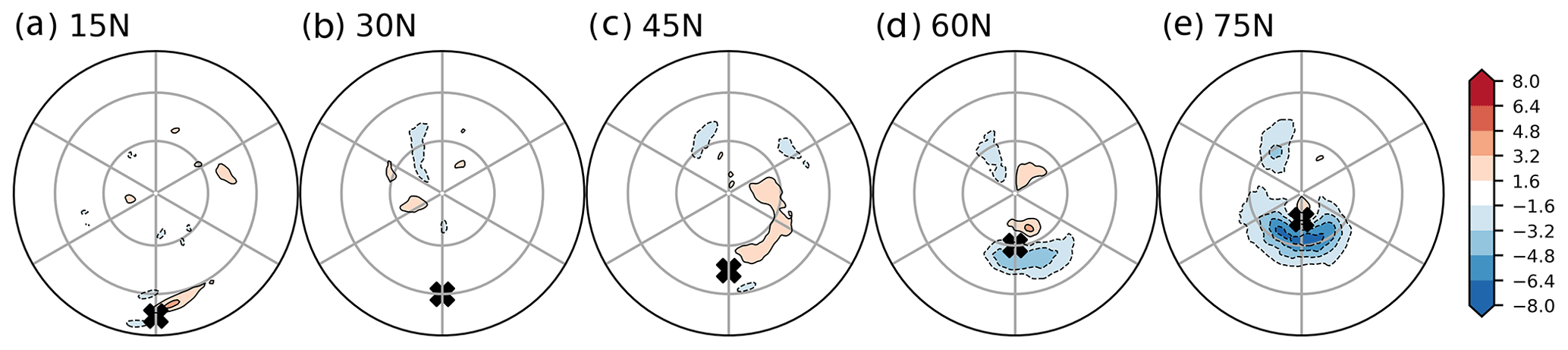
Figure 8Near-surface (990 hPa) meridional transient eddy heat flux response (, K ms−1) in the (a) 15° N, (b) 30° N, (c) 45° N, (d) 60° N, and (e) 75° N heating perturbation experiments. The crosses mark the positions of the surface heating perturbations. The latitude lines mark 30 and 60° N. The longitude lines denote 60° intervals, marking 120° W, 60° W, 0°, 60° E, 120° E, and 180°.
3.4 Contrasting dynamical and radiative adjustment processes
Results to this point show the combinations of circulation processes that are responsible for the dynamical adjustment to heating perturbations at different latitudes. Vertical motion plays the dominant role in balancing heating at low latitudes, while divergence of transient eddy heat flux plays the dominant role at high latitudes. However, these analyses do not speak to why diabatic heating (Fig. 6, top row) and the temperature response (Figs. 2 and 3) differ as the heating source is moved from low to high latitudes. To investigate this, we turn to radiative cooling, which is hypothesised to be important in the adjustment of polar regions to energy input (Kim et al., 2021; Woollings et al., 2023; Miyawaki et al., 2023). In this case, a heating perturbation is balanced by enhanced longwave emission due to an increase in atmospheric temperature. Assessing the relative importance of dynamical processes compared to radiative and turbulent fluxes requires us to move from the thermodynamic equation (see Sect. 2.3) to a moist static energy budget of the atmospheric column above the heating source (see Sect. 2.4).
Energy input to the atmospheric column from the Q-flux heating perturbation is accomplished via anomalous upward fluxes of sensible (Fig. 9, red) and latent (orange) heat as well as net longwave radiation (upwards minus downwards; yellow). While the sum of these surface fluxes inputs the same total amount of anomalous energy into the atmosphere across the perturbation experiments (around 40 W m−2), the partitioning depends on the latitude of the heating. Latent heat fluxes contribute the most in all experiments, ranging from 93 % of the total input for the 15° N heating source to 52 % for the 75° N heating source. The decrease in latent heat input is compensated by an increase in sensible heat fluxes and net longwave radiation. Note that shortwave radiation is not shown because it remains unchanged from the control to perturbation experiments due to the idealised model setup (i.e. no changes in clouds, ice, or albedo).
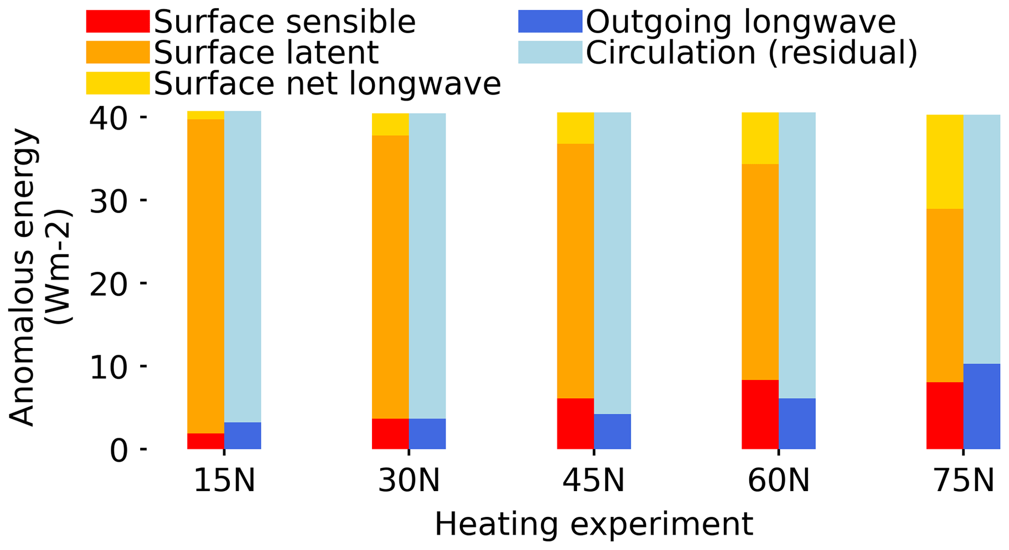
Figure 9Anomalous energy (W m−2) entering (warm colours, left bars) and leaving (cold colours, right bars) the atmospheric column above the heating perturbations compared to the control experiment, averaged over the domain of the heating perturbation. Energy entering the atmospheric column from the surface includes the net longwave radiation (yellow) and surface latent (orange) and sensible (red) heat fluxes. Energy leaving the atmospheric column includes the outgoing longwave radiation (dark blue) and the horizontal transport of moist static energy (light blue).
At equilibrium, the anomalous energy entering the atmospheric column from the surface is balanced by anomalous radiative cooling at the top of the atmosphere (outgoing longwave radiation; dark blue) and horizontal energy transport out of the column by the circulation (i.e. the advection and transient terms discussed in previous subsection, treated here as a residual; light blue). The horizontal energy transport by the circulation plays a more important role than radiative cooling in removing the excess energy locally for all experiments. However, the circulation contribution becomes weaker as the heating is moved further north, and a larger part of the excess energy must be balanced by longwave emission from the top of the atmosphere. An increased reliance on radiative cooling in the balance suggests an amplified temperature response to heating at the poles compared to the tropics (Figs. 2 and 3) according to the Stefan–Boltzmann law (i.e. longwave emission is proportional to , where Te is the emission temperature). Such a non-linear relationship further indicates that a larger temperature change is required to emit the same amount of longwave radiation in the colder polar regions than in the tropics (see Henry and Merlis, 2019), which is seen from our experiments as well. For example, the 75° N (15° N) heating experiment shows a 5.5 K (0.8 K) averaged surface warming with a 10.3 W m−2 (3.2 W m−2) increase in outgoing longwave radiation over the heating source, indicating an additional 1.9 W m−2 (4 W m−2) of longwave emission per degree of surface temperature increase. This is consistent with less-negative Planck feedback that leads to Arctic amplification of warming under globally uniform heating of well-mixed greenhouse gas forcing (Henry and Merlis, 2019).
A few additional considerations bear mentioning in explaining the structure of the response to high-latitude heating compared to low-latitude heating. At lower latitudes, vertical advection efficiently moves heat away from the surface and maximises warming in the upper troposphere (Fig. 3a). This increases the efficiency of radiative cooling to space, providing negative feedback to the surface warming. Conversely, at high latitudes, the lack of vertical advection in moving heat away from the surface implies a bottom-heavy temperature profile (Fig. 3e). This steepens the lapse rate and reduces the efficiency of radiative cooling to space, producing positive feedback that requires more surface warming to restore energy balance (Bintanja et al., 2011; Graversen et al., 2014; Pithan and Mauritsen, 2014; Feldl et al., 2020; Boeke et al., 2021). Overall, the dynamical and radiative adjustments contribute to the amplified surface warming for the high-latitude heating experiment.
In this study, we build on the foundational work of Hoskins and Karoly (1981), exploring the atmospheric circulation response to low latitude and midlatitude surface heating. We revisit their study using a moist grey radiation model, and expand the focus to surface heating perturbations at all latitudes from the tropics to the poles. Heating at low latitudes to midlatitudes is offset mainly by time-mean vertical and horizontal potential temperature advection, respectively, consistent with Hoskins and Karoly (1981). Additionally, we explore the response to heating at high latitudes, and find that the dominant contribution to balancing the heating perturbation is by transient eddies rather than the time-mean circulation. Overall, however, the circulation (time-mean plus transient) response at high latitudes is less efficient at removing near-surface heat compared to the circulation response at lower latitudes. Associated with the weaker circulation contribution at high latitudes is a stronger contribution from radiative cooling, leading to an amplified surface and near-surface temperature response. Thus, our idealised modelling results are relevant to understanding the link between surface heating arising from Arctic sea ice loss (analogous to the Q-flux perturbation at 75° N in our idealised setup) and the Arctic amplification of surface warming seen in observations and comprehensive climate models.
Why is the circulation response less efficient in balancing imposed heating at higher latitudes compared to lower latitudes? We hypothesise that the circulation response is more-tightly linked to the surface temperature response for the high-latitude case. Specifically, the reduced meridional eddy heat transport (Fig. 8) is set up by the amplified surface warming via a reduction in baroclinicity (Fig. S6). Such a strong dependence limits how much the reduced eddy activity can cool the perturbation region. At lower latitudes, time-mean circulation responses (vertical and horizontal advection) that act to balance the lower-latitude heating are less dependent on the temperature response.
However, future studies should test whether these results are sensitive to the addition of processes that are missing in our idealised setup, including clouds (Kay and Gettelman, 2009; Huang et al., 2021), radiative effect (Tan et al., 2019; Jucker and Gerber, 2017), water vapour, and ice–albedo feedback (e.g. Beer and Eisenman, 2022; Chung and Feldl, 2024; Feldl and Merlis, 2023). Future studies could test the role of these additional processes using the Isca modelling framework (Vallis et al., 2018), which allows one to increase the model's complexity step-by-step by adding sea ice, clouds, topography, a realistic radiative scheme, etc.
Finally, we note that the dynamical and radiative adjustments arising from the perturbations simultaneously shape the temperature responses. As such, our experimental design cannot fully disentangle the cause of the amplified surface temperature response in the “Arctic” heating experiments. A carefully designed experiment with abruptly switched-on surface heating with large-ensemble members (similar to the setup in Deser et al., 2007; Hell et al., 2020) but looking at the day-to-day temporal evolution of the dynamic and radiative responses could be helpful in better determining the causal relations than looking at the equilibrium responses as was done here. Additionally, incrementally adding dynamic and radiative components into an idealised model might be useful to isolate their individual roles (e.g. Feldl and Merlis, 2021).
The code to construct all figures is available online at: https://github.com/PeterSiew/SiewEA2024_circulation (Siew, 2024).
All data in this study are available upon request.
The supplement related to this article is available online at: https://doi.org/10.5194/wcd-5-985-2024-supplement.
PYFS performed the model simulations, conducted the analysis, prepared the figures, and wrote the paper with contributions from all co-authors. PYFS, CL, and SPS conceived of the original idea. CL, SPS, EDS, and MT provided guidance on the interpretation of results.
At least one of the (co-)authors is a member of the editorial board of Weather and Climate Dynamics. The peer-review process was guided by an independent editor, and the authors also have no other competing interests to declare.
Publisher's note: Copernicus Publications remains neutral with regard to jurisdictional claims made in the text, published maps, institutional affiliations, or any other geographical representation in this paper. While Copernicus Publications makes every effort to include appropriate place names, the final responsibility lies with the authors.
We acknowledge the Isca modelling group from the University of Exeter for providing the model framework and acknowledge support from the Norwegian research infrastructure services (NRIS) Sigma2 for computing resources. We thank Michael Previdi, Paul Kushner, Tim Woollings, Tyler Janoski, and Yutian Wu for useful discussions.
This work was supported by Research Council of Norway projects 255027 (DynAMiTe), 276730 (Nansen Legacy), and 295046 (KeyCLIM) and by the EMULATE project funded through the Bjerknes Centre for Climate Research by the Norwegian Department of Education. Funding for Mingfang Ting was provided by the National Science Foundation, grant no. AGS 1934358.
This paper was edited by Nili Harnik and reviewed by three anonymous referees.
Beer, E. and Eisenman, I.: Revisiting the role of the water vapor and lapse rate feedbacks in the Arctic amplification of climate change, J. Climate, 35, 2975–2988, https://doi.org/10.1175/JCLI-D-21-0814.1, 2022. a
Bintanja, R., Graversen, R., and Hazeleger, W.: Arctic winter warming amplified by the thermal inversion and consequent low infrared cooling to space, Nat. Geosci., 4, 758–761, https://doi.org/10.1038/ngeo1285, 2011. a
Boeke, R. C., Taylor, P. C., and Sejas, S. A.: On the nature of the Arctic's positive lapse-rate feedback, Geophys. Res. Lett., 48, e2020GL091109, https://doi.org/10.1029/2020GL091109, 2021. a
Butler, A. H., Thompson, D. W., and Heikes, R.: The steady-state atmospheric circulation response to climate change–like thermal forcings in a simple general circulation model, J. Climate, 23, 3474–3496, https://doi.org/10.1175/2010JCLI3228.1, 2010. a
Chung, P.-C. and Feldl, N.: Sea ice loss, water vapor increases, and their interactions with atmospheric energy transport in driving seasonal polar amplification, J. Climate, 37, 2713–2725, https://doi.org/10.1175/JCLI-D-23-0219.1, 2024. a
Cohen, J., Screen, J. A., Furtado, J. C., Barlow, M., Whittleston, D., Coumou, D., Francis, J., Dethloff, K., Entekhabi, D., Overland, J., and Jones, J.: Recent Arctic amplification and extreme mid-latitude weather, Nat. Geosci., 7, 627–637, https://doi.org/10.1038/ngeo2234, 2014. a, b
Cohen, J., Zhang, X., Francis, J., Jung, T., Kwok, R., Overland, J., Ballinger, T., Bhatt, U., Chen, H., Coumou, D., Feldstein, S., Gu, H., Handorf, D., Henderson, G., Ionita, M., Kretschmer, M., Laliberte, F., Lee, S., Linderholm, H. W., Maslowski, W., Peings, Y., Pfeiffer, K., Rigor, I., Semmler, T., Stroeve, J., Taylor, P. C., Vavrus, S., Vihma, T., Wang, S., Wendisch, M., Wu, Y., and Yoon, J.: Divergent consensuses on Arctic amplification influence on midlatitude severe winter weather, Nat. Clim. Change, 10, 20–29, https://doi.org/10.1038/s41558-019-0662-y, 2020. a, b
Dai, A., Luo, D., Song, M., and Liu, J.: Arctic amplification is caused by sea-ice loss under increasing CO2, Nat. Commun., 10, 121, https://doi.org/10.1038/s41467-018-07954-9, 2019. a
Deser, C., Magnusdottir, G., Saravanan, R., and Phillips, A.: The effects of North Atlantic SST and sea ice anomalies on the winter circulation in CCM3. Part II: Direct and indirect components of the response, J. Climate, 17, 877–889, https://doi.org/10.1175/1520-0442(2004)017<0877:TEONAS>2.0.CO;2, 2004. a
Deser, C., Tomas, R. A., and Peng, S.: The transient atmospheric circulation response to North Atlantic SST and sea ice anomalies, J. Climate, 20, 4751–4767, https://doi.org/10.1175/JCLI4278.1, 2007. a, b, c
Deser, C., Tomas, R., Alexander, M., and Lawrence, D.: The seasonal atmospheric response to projected Arctic sea ice loss in the late twenty-first century, J. Climate, 23, 333–351, https://doi.org/10.1175/2009JCLI3053.1, 2010. a
Dunn-Sigouin, E., Li, C., and Kushner, P.: Limited Influence of Localized Tropical Sea-Surface Temperatures on Moisture Transport into the Arctic, Geophys. Res. Lett., 48, e2020GL091540, https://doi.org/10.1029/2020GL091540, 2021. a
England, M. R., Eisenman, I., Lutsko, N. J., and Wagner, T. J.: The recent emergence of Arctic Amplification, Geophys. Res. Lett., 48, e2021GL094086, https://doi.org/10.1029/2021GL094086, 2021. a, b
Feldl, N. and Merlis, T. M.: Polar amplification in idealized climates: The role of ice, moisture, and seasons, Geophys. Res. Lett., 48, e2021GL094130, https://doi.org/10.1029/2021GL094130, 2021. a
Feldl, N. and Merlis, T. M.: A Semi-Analytical Model for Water Vapor, Temperature, and Surface-Albedo Feedbacks in Comprehensive Climate Models, Geophys. Res. Lett., 50, e2023GL105796, https://doi.org/10.1029/2023GL105796, 2023. a
Feldl, N., Po-Chedley, S., Singh, H. K., Hay, S., and Kushner, P. J.: Sea ice and atmospheric circulation shape the high-latitude lapse rate feedback, NPJ Clim. Atmos. Sci., 3, 41, https://doi.org/10.1038/s41612-020-00146-7, 2020. a
Frierson, D. M.: The dynamics of idealized convection schemes and their effect on the zonally averaged tropical circulation, J. Atmos. Sci., 64, 1959–1976, https://doi.org/10.1175/JAS3935.1, 2007. a
Frierson, D. M., Held, I. M., and Zurita-Gotor, P.: A gray-radiation aquaplanet moist GCM. Part I: Static stability and eddy scale, J. Atmos. Sci., 63, 2548–2566, https://doi.org/10.1175/JAS3753.1, 2006. a, b
Graversen, R. G., Langen, P. L., and Mauritsen, T.: Polar amplification in CCSM4: Contributions from the lapse rate and surface albedo feedbacks, J. Climate, 27, 4433–4450, https://doi.org/10.1175/JCLI-D-13-00551.1, 2014. a
Hall, N. M., Derome, J., and Lin, H.: The extratropical signal generated by a midlatitude SST anomaly. Part I: Sensitivity at equilibrium, J. Climate, 14, 2035–2053, https://doi.org/10.1175/1520-0442(2001)014<2035:TESGBA>2.0.CO;2, 2001. a
Hell, M. C., Schneider, T., and Li, C.: Atmospheric circulation response to short-term Arctic warming in an idealized model, J. Atmos. Sci., 77, 531–549, https://doi.org/10.1175/JAS-D-19-0133.1, 2020. a, b, c
Henry, M. and Merlis, T. M.: The role of the nonlinearity of the Stefan–Boltzmann law on the structure of radiatively forced temperature change, J. Climate, 32, 335–348, https://doi.org/10.1175/JCLI-D-17-0603.1, 2019. a, b
Hoskins, B. and Woollings, T.: Persistent extratropical regimes and climate extremes, Curr. Clim. Change Rep., 1, 115–124, https://doi.org/10.1007/s40641-015-0020-8, 2015. a
Hoskins, B. J. and Karoly, D. J.: The steady linear response of a spherical atmosphere to thermal and orographic forcing, J. Atmos. Sci., 38, 1179–1196, 1981. a, b, c, d, e, f, g, h, i, j, k, l, m, n
Huang, Y., Ding, Q., Dong, X., Xi, B., and Baxter, I.: Summertime low clouds mediate the impact of the large-scale circulation on Arctic sea ice, Commun. Earth Environ., 2, 38, https://doi.org/10.1038/s43247-021-00114-w, 2021. a
Inatsu, M., Mukougawa, H., and Xie, S.-P.: Stationary eddy response to surface boundary forcing: Idealized GCM experiments, J. Atmos. Sci., 59, 1898–1915, https://doi.org/10.1175/1520-0469(2002)059<1898:SERTSB>2.0.CO;2, 2002. a
Inatsu, M., Mukougawa, H., and Xie, S.-P.: Atmospheric response to zonal variations in midlatitude SST: Transient and stationary eddies and their feedback, J. Climate, 16, 3314–3329, https://doi.org/10.1175/1520-0442(2003)016<3314:ARTZVI>2.0.CO;2, 2003. a
James, I. N.: Introduction to circulating atmospheres, Cambridge University Press, https://doi.org/10.1017/CBO9780511622977, 1995. a
Jucker, M. and Gerber, E.: Untangling the annual cycle of the tropical tropopause layer with an idealized moist model, J. Climate, 30, 7339–7358, https://doi.org/10.1175/JCLI-D-17-0127.1, 2017. a
Kay, J. E. and Gettelman, A.: Cloud influence on and response to seasonal Arctic sea ice loss, J. Geophys. Res.-Atmos., 114, D18204, https://doi.org/10.1029/2009JD011773, 2009. a
Kim, D., Kang, S. M., Merlis, T. M., and Shin, Y.: Atmospheric circulation sensitivity to changes in the vertical structure of polar warming, Geophys. Res. Lett., 48, e2021GL094726, https://doi.org/10.1029/2021GL094726, 2021. a, b
Kim, H.-M. and Kim, B.-M.: Relative contributions of atmospheric energy transport and sea ice loss to the recent warm Arctic winter, J. Climate, 30, 7441–7450, https://doi.org/10.1175/JCLI-D-17-0157.1, 2017. a
Labe, Z., Peings, Y., and Magnusdottir, G.: Warm Arctic, cold Siberia pattern: role of full Arctic amplification versus sea ice loss alone, Geophys. Res. Lett., 47, e2020GL088583, https://doi.org/10.1029/2020GL088583, 2020. a
Langen, P. L., Graversen, R. G., and Mauritsen, T.: Separation of contributions from radiative feedbacks to polar amplification on an aquaplanet, J. Climate, 25, 3010–3024, https://doi.org/10.1175/JCLI-D-11-00246.1, 2012. a
Magnusdottir, G., Deser, C., and Saravanan, R.: The effects of North Atlantic SST and sea ice anomalies on the winter circulation in CCM3. Part I: Main features and storm track characteristics of the response, J. Climate, 17, 857–876, https://doi.org/10.1175/1520-0442(2004)017<0857:TEONAS>2.0.CO;2, 2004. a
Matthews, T., Byrne, M., Horton, R., Murphy, C., Pielke Sr., R., Raymond, C., Thorne, P., and Wilby, R. L.: Latent heat must be visible in climate communications, Wiley Interdisciplin. Rev.: Clim. Change, 13, e779, https://doi.org/10.1002/wcc.779, 2022. a
Miyawaki, O., Shaw, T., and Jansen, M.: The emergence of a new wintertime Arctic energy balance regime, Environ. Res.: Climate, 2, 031003, https://doi.org/10.1088/2752-5295/aced63, 2023. a, b, c
Mori, M., Kosaka, Y., Watanabe, M., Nakamura, H., and Kimoto, M.: A reconciled estimate of the influence of Arctic sea-ice loss on recent Eurasian cooling, Nat. Clim. Change, 9, 123–129, https://doi.org/10.1038/s41558-018-0379-3, 2019. a
O'Gorman, P. A. and Schneider, T.: The hydrological cycle over a wide range of climates simulated with an idealized GCM, J. Climate, 21, 3815–3832, https://doi.org/10.1175/2007JCLI2065.1, 2008. a, b
Olonscheck, D., Mauritsen, T., and Notz, D.: Arctic sea-ice variability is primarily driven by atmospheric temperature fluctuations, Nat. Geosci., 12, 430–434, https://doi.org/10.1038/s41561-019-0363-1, 2019. a
Outten, S., Li, C., King, M. P., Suo, L., Siew, P. Y. F., Cheung, H., Davy, R., Dunn-Sigouin, E., Furevik, T., He, S., Madonna, E., Sobolowski, S., Spengler, T., and Woollings, T.: Reconciling conflicting evidence for the cause of the observed early 21st century Eurasian cooling, Weather Clim. Dynam., 4, 95–114, https://doi.org/10.5194/wcd-4-95-2023, 2023. a
Peixoto, J. P. and Oort, A. H.: Physics of climate, American Institute of Physics, https://link.springer.com/book/9780883187128 (last access: 31 July 2024), 1992. a
Pithan, F. and Mauritsen, T.: Arctic amplification dominated by temperature feedbacks in contemporary climate models, Nat. Geosci., 7, 181–184, https://doi.org/10.1038/ngeo2071, 2014. a
Previdi, M., Smith, K. L., and Polvani, L. M.: Arctic amplification of climate change: a review of underlying mechanisms, Environ. Res. Lett., 16, 093003, https://doi.org/10.1088/1748-9326/ac1c29, 2021. a
Rantanen, M., Karpechko, A. Y., Lipponen, A., Nordling, K., Hyvärinen, O., Ruosteenoja, K., Vihma, T., and Laaksonen, A.: The Arctic has warmed nearly four times faster than the globe since 1979, Commun. Earth Environ., 3, 168, https://doi.org/10.1038/s43247-022-00498-3, 2022. a, b
Sellevold, R., Sobolowski, S., and Li, C.: Investigating possible Arctic–midlatitude teleconnections in a linear framework, J. Climate, 29, 7329–7343, https://doi.org/10.1175/JCLI-D-15-0902.1, 2016. a, b
Serreze, M., Barrett, A., Stroeve, J., Kindig, D., and Holland, M.: The emergence of surface-based Arctic amplification, The Cryosphere, 3, 11–19, https://doi.org/10.5194/tc-3-11-2009, 2009. a
Shaw, T. A. and Smith, Z.: The midlatitude response to polar sea ice loss: Idealized slab-ocean aquaplanet experiments with thermodynamic sea ice, J. Climate, 35, 2633–2649, 2022. a
Shepherd, T. G.: Effects of a warming Arctic, Science, 353, 989–990, https://doi.org/10.1126/science.aag2349, 2016. a
Siew, P. Y. F.: GitHub repository – SiewEA2024_circulation, GitHub [code], https://github.com/PeterSiew/SiewEA2024_circulation (last access: 31 July 2024), 2024. a
Siew, P. Y. F., Li, C., Sobolowski, S. P., and King, M. P.: Intermittency of Arctic-mid-latitude teleconnections: stratospheric pathway between autumn sea ice and the winter North Atlantic Oscillation, Weather Clim. Dynam., 1, 261–275, https://doi.org/10.5194/wcd-1-261-2020, 2020. a
Siew, P. Y. F., Li, C., Ting, M., Sobolowski, S. P., Wu, Y., and Chen, X.: North Atlantic Oscillation in winter is largely insensitive to autumn Barents-Kara sea ice variability, Sci. Adv., 7, eabg4893, https://doi.org/10.1126/sciadv.abg4893, 2021. a
Sun, L., Deser, C., Simpson, I., and Sigmond, M.: Uncertainty in the winter tropospheric response to Arctic Sea ice loss: The role of stratospheric polar vortex internal variability, J. Climate, 35, 3109–3130, https://doi.org/10.1175/JCLI-D-21-0543.1, 2022. a
Tan, Z., Lachmy, O., and Shaw, T. A.: The sensitivity of the jet stream response to climate change to radiative assumptions, J. Adv. Model. Earth Syst., 11, 934–956, https://doi.org/10.1029/2018MS001492, 2019. a
Thomson, S. I. and Vallis, G. K.: Atmospheric response to SST anomalies. Part I: Background-state dependence, teleconnections, and local effects in winter, J. Atmos. Sci., 75, 4107–4124, https://doi.org/10.1175/JAS-D-17-0297.1, 2018. a
Ting, M.: The stationary wave response to a midlatitude SST anomaly in an idealized GCM, J. Atmos. Sci., 48, 1249–1275, 1991. a
Ting, M. and Held, I. M.: The stationary wave response to a tropical SST anomaly in an idealized GCM, J. Atmos. Sci., 47, 2546–2566, https://doi.org/10.1175/1520-0469(1990)047<2546:TSWRTA>2.0.CO;2, 1990. a
Vallis, G. K., Colyer, G., Geen, R., Gerber, E., Jucker, M., Maher, P., Paterson, A., Pietschnig, M., Penn, J., and Thomson, S. I.: Isca, v1.0: A framework for the global modelling of the atmospheres of Earth and other planets at varying levels of complexity, Geosci. Model Dev., 11, 843–859, https://doi.org/10.5194/gmd-11-843-2018, 2018. a, b
Voigt, A., Biasutti, M., Scheff, J., Bader, J., Bordoni, S., Codron, F., Dixon, R. D., Jonas, J., Kang, S. M., Klingaman, N. P., Leung, R., Lu, J., Mapes, B., Maroon, E. A., McDermid, S., Park, J., Roehrig, R., Rose, B. E. J., Russell, G. L., Seo, J., Toniazzo, T., Wei, H., Yoshimori, M., and Zeppetello, L. R. V.: The tropical rain belts with an annual cycle and a continent model intercomparison project: TRACMIP, J. Adv. Model. Earth Syst., 8, 1868–1891, https://doi.org/10.1002/2016MS000748, 2016. a, b
Wallace, J. M., Held, I. M., Thompson, D. W., Trenberth, K. E., and Walsh, J. E.: Global warming and winter weather, Science, 343, 729–730, https://doi.org/10.1126/science.343.6172.729, 2014. a
Walter, K., Luksch, U., and Fraedrich, K.: A response climatology of idealized midlatitude thermal forcing experiments with and without a storm track, J. Climate, 14, 467–484, https://doi.org/10.1175/1520-0442(2001)014<0467:ARCOIM>2.0.CO;2, 2001. a
Winton, M.: Amplified Arctic climate change: What does surface albedo feedback have to do with it?, Geophys. Res. Lett., 33, L03701, https://doi.org/10.1029/2005GL025244, 2006. a
Woollings, T., Li, C., Drouard, M., Dunn-Sigouin, E., Elmestekawy, K. A., Hell, M., Hoskins, B., Mbengue, C., Patterson, M., and Spengler, T.: The role of Rossby waves in polar weather and climate, Weather Clim. Dynam., 4, 61–80, https://doi.org/10.5194/wcd-4-61-2023, 2023. a, b, c, d
Wu, Y. and Smith, K. L.: Response of Northern Hemisphere midlatitude circulation to Arctic amplification in a simple atmospheric general circulation model, J. Climate, 29, 2041–2058, https://doi.org/10.1175/JCLI-D-15-0602.1, 2016. a
Zhang, P., Wu, Y., and Smith, K. L.: Prolonged effect of the stratospheric pathway in linking Barents–Kara Sea sea ice variability to the midlatitude circulation in a simplified model, Clim. Dynam., 50, 527–539, https://doi.org/10.1007/s00382-017-3624-y, 2018. a
Zheng, C., Wu, Y., Ting, M., Screen, J. A., and Zhang, P.: Diverse Eurasian Temperature Responses to Arctic Sea Ice Loss in Models due to Varying Balance between Dynamic Cooling and Thermodynamic Warming, J. Climate, 36, 8347–8364, https://doi.org/10.1175/JCLI-D-22-0937.1, 2023. a