the Creative Commons Attribution 4.0 License.
the Creative Commons Attribution 4.0 License.
 | 06 Aug 2024
A linear assessment of barotropic Rossby wave propagation in different background flow configurations
Antonio Segalini
Jacopo Riboldi
Volkmar Wirth
Gabriele Messori
The horizontal propagation of Rossby waves in the upper troposphere has been a long-standing topic in dynamical meteorology. The concept of “waveguidability’’, i.e., the capability of the background flow to act as a zonal waveguide for Rossby waves, may prove useful to address this problem, but developing a systematic definition and quantification of such a property remains challenging. With an eye to such issues, the current paper suggests a novel and efficient algorithm to solve the linearized barotropic vorticity equation on a sphere in a forced-dissipative configuration. The algorithm allows one to obtain linear wave solutions resulting from arbitrary combinations of the forcing and the background zonal wind. These solutions can be used to systematically study single- and double-jet configurations and are employed here to show that the latitude of the jet stream does not appear to affect waveguidability. The onset of barotropic instability might hinder the applicability of the linear framework, but it is shown that the nonlinear flow evolution can still be retrieved qualitatively from the linearized solution, both for the stationary component of the wave field and for the temporal evolution of transient waves.
- Article
(5196 KB) - Full-text XML
- BibTeX
- EndNote


Rossby waves are a fundamental component of upper-tropospheric dynamics (Rossby, 1939, 1940) and are instrumental in modulating the location, intensity and tracks of extratropical weather systems. They can be forced by baroclinic instability, large-scale topographical features and meso- to large-scale diabatic heating (e.g., Rhines, 1975; Hoskins and Karoly, 1981; Held, 1983; Garcia and Salby, 1987; Held et al., 2002; Brayshaw et al., 2009; Garfinkel et al., 2020; Martius et al., 2021). A key characteristic of Rossby waves, which has profound implications for their modulation of weather systems, is their propagation. The Earth's spherical geometry usually leads to the equatorward refraction of Rossby waves (Hoskins and Karoly, 1981), yet the presence of localized upper-tropospheric jet streams can favor a zonal propagation (e.g., Hoskins and Valdes, 1990; Ambrizzi et al., 1995; Branstator, 2002; Wirth et al., 2018). The capability of jet streams to promote Rossby wave propagation, referred to as “waveguidability”, has long been subject of research (see the reviews by Wirth et al., 2018; White et al., 2022). Waveguides typically exist for timescales longer than the waves they “guide”, and this property can be exploited to understand the persistence and predictability of midlatitude weather (Martius et al., 2010).
The amplification and propagation of Rossby waves along such waveguides have been related in the literature to the occurrence of extreme weather events both in winter (e.g., Davies, 2015; Harnik et al., 2016; Kornhuber and Messori, 2023) and summer (e.g., Kornhuber et al., 2019; Teng and Branstator, 2019; Di Capua et al., 2021; Rousi et al., 2022; Jiménez-Esteve et al., 2022). In a number of these examples, Rossby waves were identified as quasi-stationary and associated with concurrent extremes in geographically remote regions due to the zonally extended, large-amplitude nature of the waves. The existence of quasi-stationary waves on a midlatitude waveguide has also been linked to the phenomenon of quasi-resonance, namely a constructive self-interference of the wave, which in turn may be linked to surface extreme events (Petoukhov et al., 2013; Coumou et al., 2014); however, whether or not quasi-resonance is a relevant mechanism in realistic situations is an unsolved question (Wirth and Polster, 2021).
The relevance that waveguidability plays in atmospheric dynamics, as well as its connection to surface extremes in a changing climate, has led to a renewed interest in its study (White et al., 2022). In general, waveguidability is regarded as a property of the background flow configuration in which Rossby waves are propagating. The concept of background flow is useful for decomposing the atmospheric flow into a background component that varies gradually in space and time, as well as a wave component (i.e., the Rossby waves in the present work) that varies more rapidly. The feasibility of such a decomposition inherently relies on the assumption that a clear scale separation exists between the waves and the background flow such that the former are not leaving an immediate signature on the latter. The identification of the background flow can be practically done by using time and/or zonal averages, a methodology based on the assumed linearity of the waves; however, this assumption is violated when Rossby waves reach significant meridional amplitudes, as often happens in the context of large-scale flow configurations associated with unusual or extreme weather (Wirth and Polster, 2021).
The role of specific background flow configurations in promoting waveguidability can be investigated in detail using idealized frameworks. Manola et al. (2013) and Wirth (2020) are notable examples of such work for the cases of single, localized jet streams in the Northern Hemisphere. These studies noticed that waveguidability increases with the strength of the jet and that latitudinally narrow jets are more efficient waveguides than broad jets. Steady wave patterns have been discussed by means of the ray-tracing technique (Hoskins and Karoly, 1981; Hoskins and Ambrizzi, 1993; Wirth, 2020), where the β-plane analysis of Rossby waves is extended to slowly meridionally varying background flows by means of Wentzel–Kramers–Brillouin (WKB) theory and a Mercator projection. This enabled the identification of waveguides as ridges in the so-called refractive index, drastically simplifying the problem with respect to a full eigenvalue analysis. However, the ray-tracing approach is subject to some crucial limitations. It is often implemented on a Mercator projection of the flow field, leading to distortion in the high latitudes, and the meridional and longitudinal variation in the background flow must be gradual compared to the scale of the wave. Moreover, although ray tracing can in principle be applied to transient waves, in practice it is typically used for the study of stationary waves (with the notable exception of Yang and Hoskins, 1996). One therefore loses information about how the waves are evolving in time or whether the flow will ever approach a steady state. A critical assessment of this approach was performed by Wirth (2020), albeit limited to only a few background flows. There is indeed a lack of understanding of Rossby waveguides in complex background flow configurations, such as the presence of two separate jet streams, which has been linked to summertime heat waves (“double jets”; e.g., Coumou et al., 2014; Rousi et al., 2022). Understanding waveguidability thus requires a systematic investigation of a large number of different background flows. Each case must also be investigated for different forcings to assess the flow response, and this task becomes quickly demanding in terms of computational resources and expert analysis time.
Motivated by this open challenge and by the limitations of ray-tracing theory, we extend in this paper the framework of Wirth (2020) to study the propagation of forced Rossby waves without recourse to ray tracing and avoiding the numerical integration of the underlying nonlinear equations. Specifically, we study Rossby wave evolution by solving explicitly the linearized, two-dimensional barotropic vorticity equation in terms of normal mode analysis. This enables one to inexpensively obtain solutions for any forcing under a given zonally symmetric background flow; furthermore, it allows one to study Rossby wave propagation without the limitations imposed by ray-tracing methods, such as the assumption of scale separation or the need to project the flow on a Mercator plane. Similar approaches have been previously employed to study other types of oscillatory phenomena, such as Rossby wave critical layers (Campbell and Maslowe, 1998), equatorial waves (Boyd, 1978) and gravity waves (Baldauf and Brdar, 2013). We first validate the solutions by comparing them with the output of nonlinear numerical simulations based on a spectral code built on spherical harmonics. The joint analysis of linear and nonlinear solutions further allows a detailed investigation of the stability of different wave modes, providing information about the transient evolution of the Rossby waves. In the end we use the novel algorithm in order to extend the analysis of waveguidability of idealized zonal jets beyond what has been done in previous publications. The paper is structured as follows: Sect. 2 presents the theory behind the linear approach, while its discrete implementation based on orthogonal Chebyshev polynomials is discussed in Appendix A. A comparison between linear and nonlinear calculations is discussed in Sect. 3, where different zonal wind profiles are investigated in terms of both the wave spatial structure and integrated parameters such as the waveguidability. The stationary solutions for single-jet and double-jet configurations are discussed, respectively, in Sects. 4 and 5. The paper is closed by some concluding remarks in Sect. 6.
Let us consider the two-dimensional barotropic vorticity equation on a spherical planet with radius a* (in this section dimensional quantities are indicated by means of an asterisk superscript):
where V* is the horizontal velocity field, is the Coriolis parameter and is the colatitude (associated with the latitude φ). Similarly to Hoskins and Ambrizzi (1993) and Wirth (2020), a damping term is present: this term provides a stabilizing effect that hinders a departure of the atmospheric state from the background vorticity, . F* indicates a generic forcing in space and time. By normalizing physical quantities with respect to the planetary radius a* and a characteristic velocity such that
the barotropic vorticity Eq. (1) is re-written in dimensionless form as
The choice of the characteristic velocity scale, , is arbitrary, but it should be of the same order of magnitude of the velocity field. In the considered two-dimensional case, the flow divergence is zero everywhere so that a streamfunction, Ψ, can be introduced, facilitating the determination of the velocity and vorticity field as
where λ indicates the longitude.
By assuming a zonal base flow uλ=U(θ) and uθ=0, the background vorticity, , is given by
Let us consider a perturbed state where the relative vorticity is given by . This will be associated with a streamfunction, , and velocity field
The equation governing the small perturbation is obtained by taking Eq. (3) and subtracting the base-state equation. The forcing term is not included in the background flow equation and generates a deviation from the latter. Furthermore, wave–mean-flow terms are not accounted for, implying that the perturbation flow is assumed not to modify the background flow itself. By also neglecting the nonlinear wave–wave terms, one obtains the linearized equation for the perturbation vorticity:
with
The system can be better analyzed by taking the Fourier transform in the zonal direction, defined as
leading to
where
and ℒ indicates the Laplace operator that, once discretized, becomes a matrix. By introducing the matrix B=iℒ and the streamfunction vector evaluated at the discrete colatitudes θj, the barotropic vorticity Eq. (10) is written as
where the terms composing the matrix A are grouped within the square brackets in Eq. (12) and I is the identity matrix (see Appendix A for a detailed description of how the differential operators are discretized and the matrices are constructed). Equation (12) is a linear system of ordinary differential equations in time with the streamfunction at the collocation points as unknowns. By erasing the time derivative, the equilibrium state of the linearized system is obtained as
similar to the formula provided by Hoskins and Karoly (1981). Equation (13) corresponds to the steady solution of the forced dynamical system achieved after a sufficiently long time if the system is stable (see discussion below for the flow stability analysis). Even if the system is unstable, the state described by Eq. (13) is the only one that erases the time derivative of the linearized system: thus, we choose to name it the “equilibrium solution”. Its determination is only related to the advection and dissipation of vorticity rather than the vorticity temporal evolution and can therefore be obtained in one computational step.
The solution of Eq. (12) describing the growth of an infinitesimally small perturbation (be it initiated by the forcing or by a generic initial condition) can be written as the sum of the homogeneous solution (starting from a given initial condition) plus a forced solution. By introducing a perturbation as a modal ansatz , it is possible to solve the homogeneous problem as an eigenvalue one, identifying the complex eigenvalues, ω, and the associated eigenfunctions for each azimuthal wavenumber, m. The advantage of the proposed framework is that the behavior of the system is determined from the eigenvalues of the homogeneous problem, which are independent of the forcing and have indeed general validity for a given zonal background flow. If all the complex eigenvalues have negative imaginary parts, the system is stable and will converge to the equilibrium state given by Eq. (13), while the perturbations will grow with time if at least one eigenvalue has a positive imaginary part. Thus, the sign of the imaginary part of the eigenvalues (hereafter referred to as the mode growth rate) determines whether a perturbation will grow or decay. The real part of the eigenvalues, on the other hand, is associated with phase propagation in the zonal direction. In this framework, the evolution of the perturbation is obtained as an initial value problem, drastically simplified by means of the modal analysis (details are provided in Appendix A). As a note of caution, the linearization is performed around the background state, , while the presence of the forcing shifts the equilibrium state of the system to (with ℱ−1 indicating the inverse zonal Fourier transform). The modal analysis assumes infinitesimal deviations from the equilibrium state, while here it is performed around the background flow. The two linearizations are identical when the forcing is infinitesimal, but the modal analysis is still expected to be qualitatively similar for reasonably small forcing, an hypothesis to be verified a posteriori. The choice to linearize around the background flow has the practical advantage that the Fourier decomposition can be applied to the linearized barotropic vorticity equation without the appearance of convolution terms that would hinder the separation of individual waves. Furthermore, as the forcing is not included in the modal analysis, its contribution is accounted for a posteriori, making the computational approach simpler and more insightful.
The proposed linearized framework, based on Chebyshev polynomials for the treatment of the solution in the meridional direction, is first compared with the test cases proposed by Wirth (2020) for two of the investigated zonal velocity profiles. The code has been written in Python, where Chebyshev polynomials have been implemented following Peyret (2002) and Canuto et al. (2006). In all simulations, only the dissipative term (with as in Wirth, 2020) was used to make the barotropic wave decay, and no hyperviscosity was introduced. The planetary radius was taken as 6371 km, while the planetary rotation speed was rad s−1. The linear problem has been discretized into an equal number of latitudes and longitudes without any aliasing consideration or numerical stability constraints (see Appendix A for the numerical details).
In order to check the code, an independent numerical solution of the barotropic vorticity equation has been implemented by using the spherical harmonics transform (SHT) package from Schaeffer (2013). Both the linear and nonlinear barotropic vorticity equations were implemented and compared to the results of the proposed linearized framework. A triangular truncation scheme was adopted with an aliasing-removal approach in both the linear and nonlinear simulations with spherical harmonics. A leapfrog scheme was used for the temporal discretization with a time step of 10 min. A Robert Asselin filter with filter parameter 0.01 was implemented to eliminate the spurious computational mode associated with the leapfrog method (Kalnay, 2003).
Since the topographic forcing F is stationary, the constant forcing solution provided by Eq. (A7) is used. The expression is further simplified here as the initial perturbation streamfunction is assumed to be zero, implying the vanishing of the first term of Eq. (A7) so that only the forced response needs to be computed. The forced response is obtained from the method of variation of constants and therefore facilitated by the eigenfunctions calculated from the homogeneous problem.
In the special case of a solid-body zonal velocity profile, , the zonal velocity is obtained as if the atmosphere was rotating at a slightly higher angular velocity than Ω and the linearized homogeneous barotropic vorticity Eq. (7) reduces to
Equation (14) can be solved analytically by means of the ansatz , where is the spherical harmonic with degree l and order m. The resulting dispersion relationship is
which is a well-known analytical result for Rossby–Haurwitz waves (Haurwitz, 1940). The attenuation parameter χ makes the eigenvalues stable, while the first term of Eq. (15) is associated with the zonal phase propagation of the wave, similarly to the planar case. From this analysis it is already known that (i) all the modes of the solid-body zonal velocity case are stable (since χ>0), (ii) the modes are spherical harmonics and (iii) the dispersion relationship is given by Eq. (15). Simulations done with different grid resolutions showed an excellent agreement between the analytical relationship (Eq. 15) and the numerical eigenvalues, with error comparable to the precision of the machine (not shown).
Figure 1a shows the meridional velocity field (positive northward) and the associated wave pattern at the equilibrium state (Eq. 13) forced by a smooth, idealized mountain located at latitude φF=45° N and longitude λF=30° E and described by
where , hF=0.3 and , unless otherwise stated. The zonal background flow is given by U=15 cos φ m s−1 (or with U0=15 m s−1 as above). Figure 1a should be compared to the nonlinear solution in Fig. 3a of Wirth (2020): the structure of the wave pattern is very similar, although here obtained without any time integration since the flow will in time approach the steady-state solution because the eigenvalue growth rate is negative.
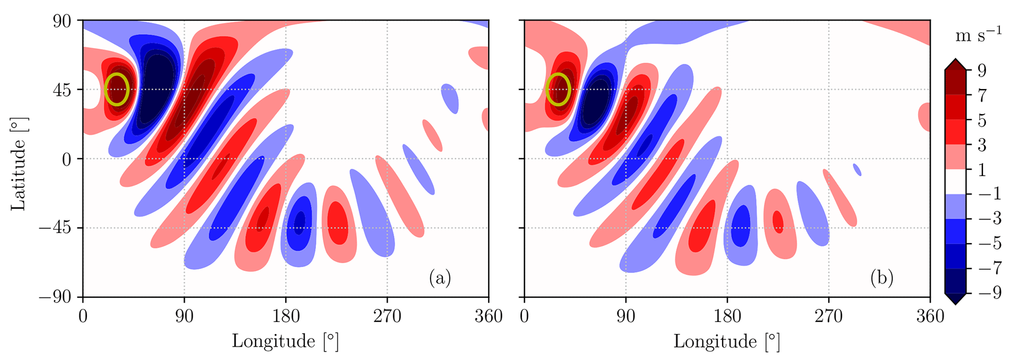
Figure 1Meridional velocity pattern at the equilibrium state for the zonal velocity profile U=15cos φ m s−1 from the linear analysis (a) and after 100 d with the nonlinear solver (b). The ellipse indicates the topographic forcing.
The linear spherical harmonics solution is practically identical to the Chebyshev approach, and therefore the results will not be shown here. The nonlinear solver has slight differences from the linear method, such as a more rapid wave attenuation away from the forcing (as visible in Fig. 1b).
A sensitivity study can be performed for different grid resolutions to assess the appropriate number of polynomials to be used in order to achieve the desired convergence. The waveguidability, as defined in Wirth (2020), has been used here as the key quantity for the comparison. The estimate by Wirth (2020) corresponds to the ratio between the enstrophy found in a monitoring region downstream of the forcing (30 and 60° N, 180 and 270° E) and the total enstrophy integrated over all latitudes across 180 and 270° E. Figure 2a shows the convergence of the waveguidability metric around 45° N for different grid resolutions in order to quantify the minimum number of polynomials needed for numerical convergence. It is noteworthy that the convergence of the results is obtained even for moderate resolutions with the linear Chebyshev and linear SHT simulations, while the nonlinear simulation approaches a higher value of the waveguidability metric, suggesting a difference between linear and nonlinear analyses. Having assessed the grid convergence, the rest of the work will use grid resolution N=256 for the solution of the linearized eigenvalue problem via Chebyshev polynomials, while a T170 truncation will be used for the nonlinear spherical harmonics simulations. Since the linear Chebyshev and the linear SHT code agree with each other and are both based on Eq. (7), only the Chebyshev implementation will be discussed in the following and it will be referred to as the linear simulation. The only nonlinear implementation of Eq. (3) is by means of the SHT, which will be hereafter denoted simply as the nonlinear simulation.
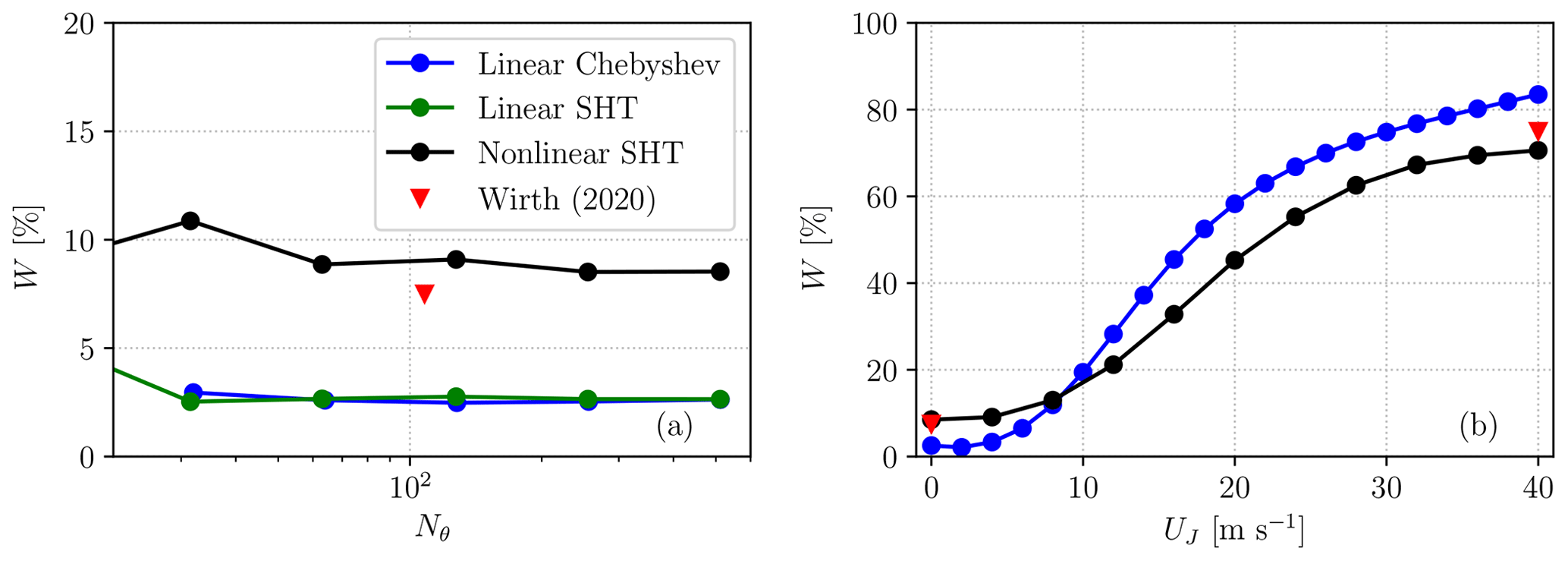
Figure 2(a) Waveguidability for a Gaussian mountain located at φF=45° N estimated from different linear and nonlinear simulations at different grid resolutions when (namely without any latitudinally confined jet). Nθ indicates the number of latitude grid points. (b) Waveguidability assessed for the linear and nonlinear simulations for Nθ=256 (corresponding to a T170 resolution) for different jet velocities UJ (according to the zonal velocity profile given in Eq. 17).
We will now focus on the case of a latitudinally confined jet described by
where UJ is the jet velocity, , φJ=45° N is the jet latitude and σJ=5° (unless otherwise stated). L indicates a linear correction that imposes U=0 at the two poles.
With this setup, we notice that the linear method is capable of replicating the waveguidability increase with jet speed, obtaining similar values as Wirth (2020) for a jet located at 45° N (Fig. 2b). Interestingly, the linear method features a convergence of the solution only for not-too-high jet speeds: in particular, for a speed faster than 20 m s−1, some of the eigenvalues λi have a positive growth rate and lead to divergence. The reasons for this behavior and the usefulness of the linear method even in such a case will be illustrated in Sect. 4.1 and 4.2.
The difference in the waveguidability metric between the linear and nonlinear solutions must be related to a stabilizing effect of the nonlinear terms (accounting for the effect of the waves on other waves and the basic state), neglected in the linear analysis. The Wirth (2020) waveguidability metric, however, cannot be easily applied to compare waveguides located at different latitudes: in fact, the physical distance between the forcing and the monitoring sector would vary when the jet latitude is changed, leading to a spurious increase in waveguidability towards the pole. An adapted metric will be proposed in Sect. 5.1 in the attempt to provide a definition able to account for jets at different latitudes.
4.1 Stability analysis
As noticed by Wirth (2020), the strong-jet case with UJ=40 m s−1 is characterized by an unsteady velocity field that does not achieve a steady state, regardless of the integration time. This unsteady behavior is partly explained by the eigenvalues provided by the linear analysis: some eigenvalues have a positive growth rate, and, therefore, the flow field is unstable. According to linear theory, the atmospheric state should diverge exponentially from the equilibrium state (shown in Fig. 3a), and each unstable Rossby wave should grow without bounds. The nonlinear simulation, however, does not display such an unrealistic divergence of wave amplitudes, and the time-averaged field, shown in Fig. 3b, remains close to the linear estimation. A great-circle wave propagation is still present as in the solid-body velocity case, as well as a wave pattern in the zonal direction of the waveguide corresponding to the strong jet.

Figure 3Meridional velocity in the strong-jet case () from the linear method at the equilibrium state (a). Meridional velocity field averaged between 10 and 100 d from the simulation start with the nonlinear solver (b). The ellipse indicates the topographic forcing.
We conduct here a systematic linear and nonlinear stability analysis to identify at what jet velocity and width unsteady traveling-wave patterns begin to appear. The Rayleigh stability criterion provides a necessary condition for the onset of barotropic instability, namely a change in sign of the absolute vorticity gradient . Since linear dissipation is present in the current problem, we slightly modify the Rayleigh criterion such that, whenever the absolute vorticity gradient changes sign, the imaginary part of ω can be different than −χ: this implies an ample stability margin before the actual onset of the linear instability (namely when the imaginary part of ω becomes positive with a positive growth rate). This result pinpoints the role of dissipation in retarding the onset of barotropic instability, confirming that the Rayleigh criterion provides a necessary but not sufficient condition for the onset of instability (Kuo, 1949).
Let us consider first the results of the eigenvalue analysis for a narrow zonal jet profile (σJ=5°) over an array of different jet speeds UJ and latitudes φJ, shown in Fig. 4a. At low UJ, the growth rate of the most unstable eigenvalue corresponds to the dissipation rate, χ, which is negative (meaning that perturbations are dampened with the same rate). This assertion is valid as long as the absolute vorticity gradient has the same sign throughout the domain. As the sign starts to flip (dashed line in Fig. 4a), a transitional regime is reached where the eigenvalue growth rate is still negative but not as low as −χ. This is related to the fact that, in the presence of dissipation, the simple change in sign of the vorticity gradient (i.e., the Rayleigh–Kuo criterion) is not sufficient to ensure the onset of barotropic instability. As UJ increases, the stability margin decreases, and above 15–22 m s−1 (depending on the jet latitude) the growth rate of at least one eigenvalue becomes positive, leading to the divergence of the linear solution (bold black line in Fig. 4a). The nonlinear simulations, on the other hand, approach divergence for larger jet velocities than for the linear method: this is marked by the green line in Fig. 4a, denoting the locus where the meridional velocity time variance equals 2 m2 s−2 as an arbitrary threshold. Above such a threshold, the velocity variance increases drastically, and it is concentrated at the jet location irrespective of the forcing, indicating the presence of barotropic instability. The neutral curve from the linear stability analysis provides then only a conservative estimate of the onset of instability: this underlines the stabilizing role of nonlinear terms (such as wave–wave and wave–mean-flow interactions) not included in the linear method.
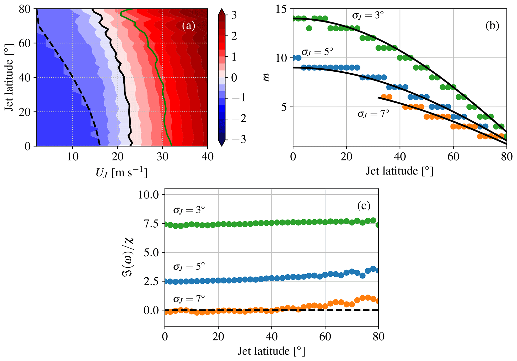
Figure 4(a) Maximum growth rate of the linear eigenvalues for a given jet velocity (normalized by χ) when σJ=5°. The solid black line indicates the neutral curve, the dashed line is the locus where the absolute vorticity gradient changes sign (Rayleigh stability criterion), and the green line is the locus beyond which the temporal variance of the meridional velocity in the nonlinear simulation becomes larger than 2 m2 s−2 (the chosen threshold for defining the neutral curve in the nonlinear case). (b) Azimuthal wavenumber of the most unstable eigenvalue for UJ=40 m s−1 for different jet widths and latitudes. The black lines in (b) are curves m∝cos φJ fitting the linear stability results. (c) Growth rate of the most unstable wave normalized by χ for UJ=40 m s−1 for different jet widths and latitudes. The dashed black line marks the boundary between the stable region (underneath) and the unstable region (above).
It is also interesting to monitor the wavenumber associated with the most unstable eigenvalue. Beyond the onset of the linear instability, this wavenumber does not depend on UJ, and therefore the wavenumber associated with the maximum growth rate in Fig. 4b is only shown for UJ=40 m s−1, where the jet is unstable at all latitudes (see Fig. 4a). For φJ=45° N a wavenumber m=6 is the most unstable, the wavenumber typical of midlatitude Rossby waves. However, as the jet is shifted to the pole, the most unstable wavenumber systematically decreases following the cosine of φJ. It is possible to explain this trend by assuming that the instability is associated with a wavelength independent of the latitude, given by
so that the wavenumber is indeed proportional to cos φ. This implies that the most barotropically unstable Rossby wave has the same wavelength at different latitudes for a zonal jet of a given width. As the jet width increases, the fixed wavelength L increases too, leading to the decrease in the most unstable zonal wavenumber m with σJ visible in Fig. 4b.
The width of the jet also modulates the onset of instability in the considered setup, with narrow jets being more prone to barotropic instability than wide jets (Fig. 4c). This behavior is related to the large meridional vorticity gradients associated with narrow jets and is illustrated in Fig. 4c by the rapid increase in the growth rate of the most unstable wave for decreasing values of σJ. Such a connection between jet width, growth rate and zonal wavelength of the most unstable wave is consistent with previous studies about barotropic-like instabilities (e.g., in the context of frontal instability, Joly and Thorpe, 1990; Leutwyler and Schär, 2019). The growth rate at fixed σJ also seems to exhibit a weak latitudinal dependence, likely related to the decrease in β towards the poles facilitating the onset of instability (see Gill, 1982, Sect. 13.6).
4.2 Wave evolution in the linearly unstable regime
After having mapped the conditions that determine the onset of instability and related them to the onset of barotropic instability, we describe here the type of instability present in the model at high jet speeds. The linear eigenvalue analysis points out that the equilibrium state given by Eq. (13) is indeed unstable. Nevertheless, such an unstable equilibrium state resembles quite closely the time-averaged nonlinear solution, which is bounded and characterized by the averaged field reported in Fig. 3b. This is noteworthy because it points to a possible usefulness of the linear approach even outside the expected range of applicability dictated by the stability analysis. Beyond the linearly stable range, only the nonlinear simulations can provide information about the flow evolution and whether or not an equilibrium state is achieved. In order to shed some light, an empirical orthogonal function (EOF) approach has been applied to the nonlinear simulation for a single jet with UJ=40 m s−1 and φJ=45° N. The EOF algorithm was applied on the meridional velocity field between 10 and 100 d after the start of the simulation without removing the time average. This provided a set of modes orthogonal to each other, including the time-averaged one, which facilitates the development of a reduced-order model of the velocity field. The corresponding modes are shown in Fig. 5 to highlight the most energetic scales governing the temporal flow evolution. The first mode is practically constant in time and remains close to the time-averaged field of the nonlinear simulation, while the second and third, fourth and fifth, and sixth and seventh modes organize themselves to create traveling-wave patterns with zonal wavenumbers m=5, m=6 and m=7, respectively (the sixth and seventh modes are not shown). These first seven modes contain 60 % of the meridional velocity variance. The modal coefficients of modes 2 and 3 are in quadrature with each other and similarly for modes 4 and 5. The trajectories in the plane spanned by the corresponding temporal coefficients, shown in Fig. 6, belong to a closed orbit and behave as traveling waves: the presence of closed orbits is also a nonlinear behavior, which is however different from the exponential growth in wave magnitude expected from the positive growth rates calculated from the linear framework. This observation suggests that a nonlinear adjustment takes place after the onset of the unstable wave growth, leading to an interplay between several nonlinear traveling waves maintaining the flow around an equilibrium state (Hou and Farrell, 1986; Lachmy and Harnik, 2016).
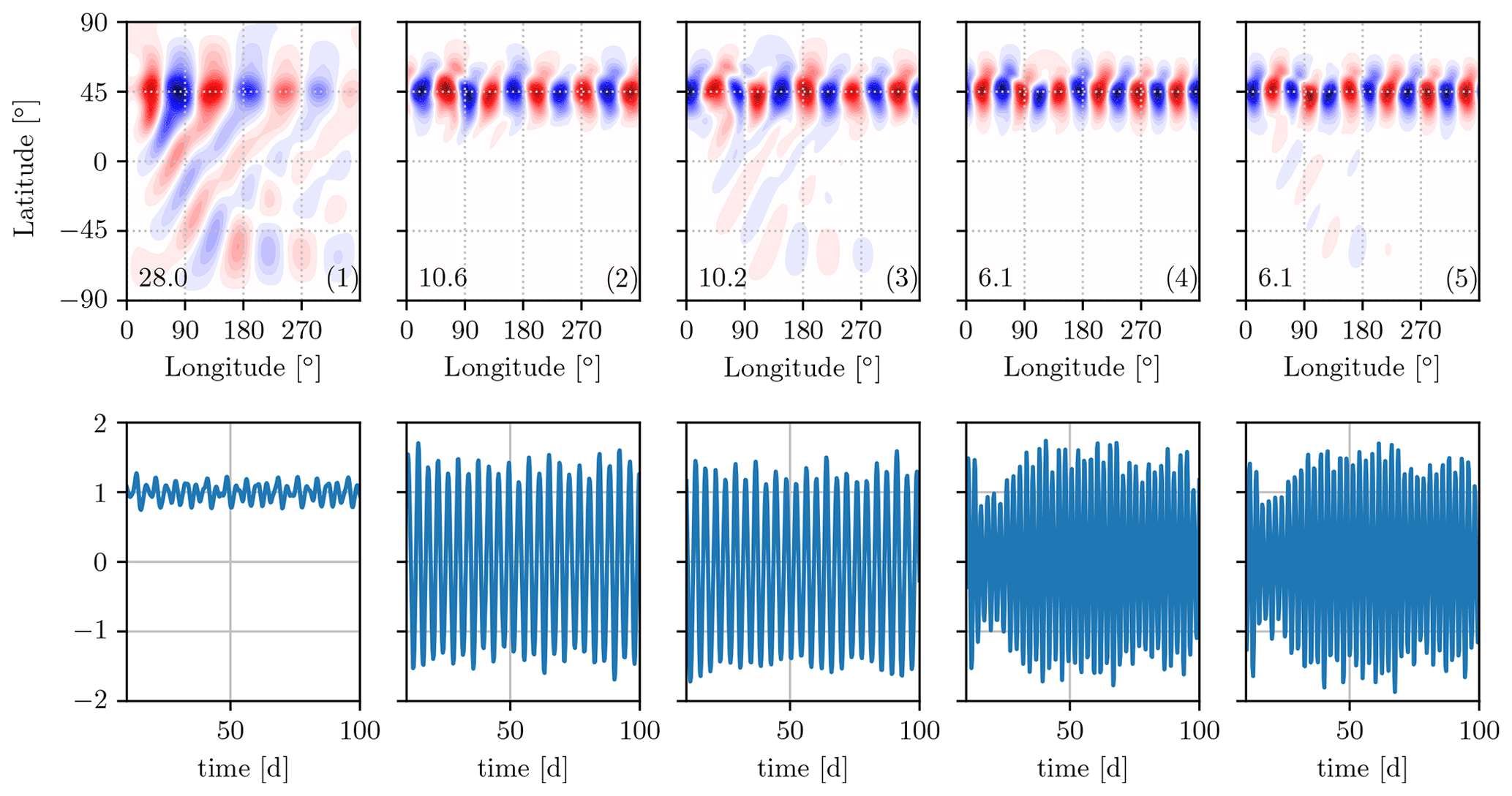
Figure 5First five modes of the EOF decomposition of the meridional velocity field obtained from the nonlinear simulations (top) and their temporal coefficient normalized by their root mean square value (bottom) for the strong-jet case with UJ=40 m s−1. The number in the bottom-left corner of the first row indicates the energy contribution of each mode in percent. The color scale in the top row is not consistent between the different modes since each mode has unitary norm.
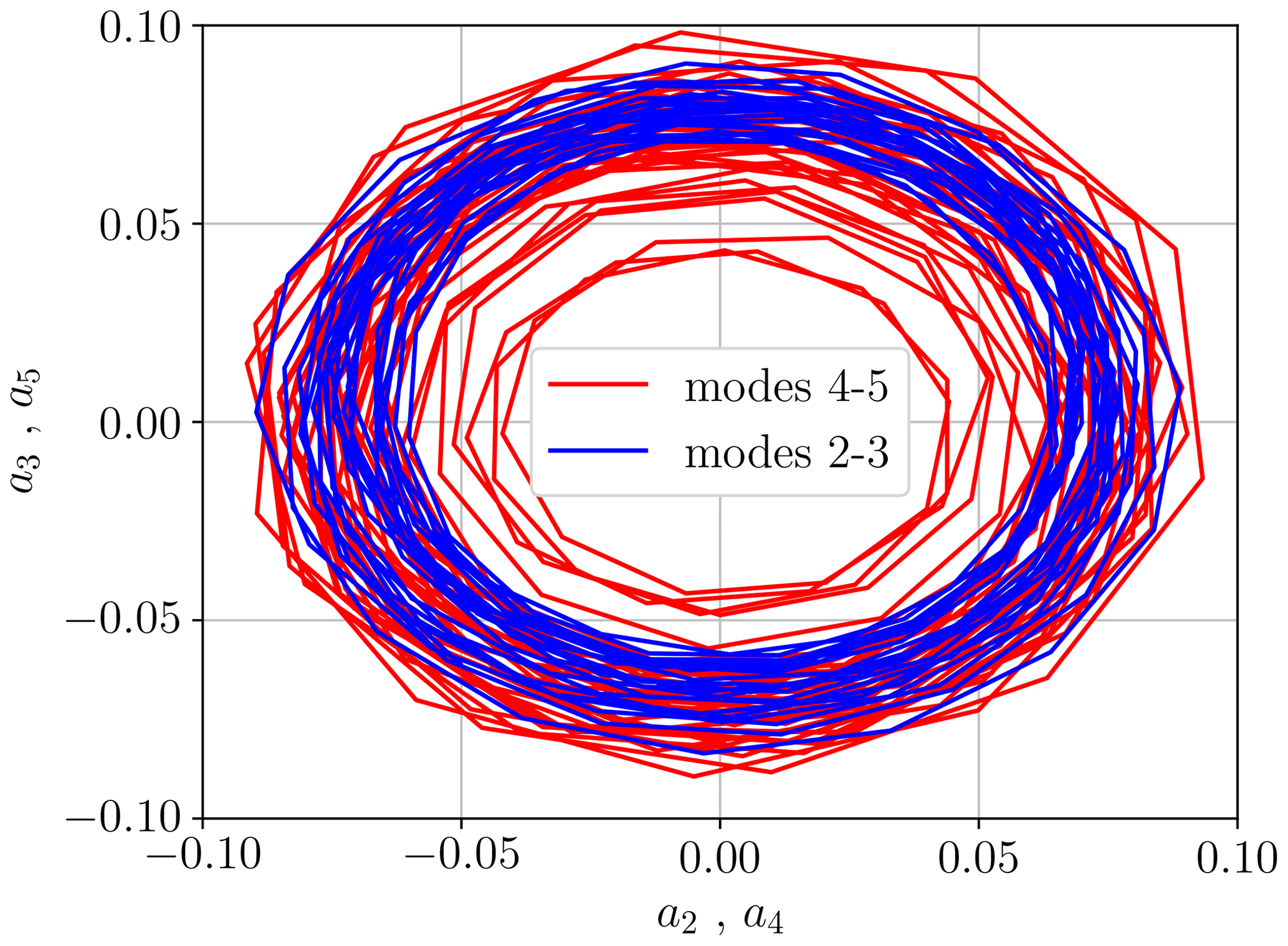
Figure 6Evolution of the temporal coefficient of mode 2 (4) plotted against the one of mode 3 (5) from the EOF analysis shown in Fig. 5. The temporal coefficients have been normalized by their root mean square.
Additional simulations where the orographic forcing was moved to lie right on the Equator did not change this overall picture, and the traveling waves (i.e., the EOF modes beyond the mean component) remained at the jet latitude (not shown). This implies that the wave components described by the EOF analysis are traveling waves determined just by the background flow rather than by the forcing, similarly to what is suggested by the linear analysis. One might wonder if there is a correspondence between the unstable modes of the linear analysis and the most energetic EOF modes. The linear unstable waves are located at the jet latitude (Fig. 7) and have similar wavenumbers to the first EOF modes. Despite the similarity, however, the most rapidly growing mode (m=6; Fig. 7) does not exactly match the EOF patterns corresponding to modes 2 and 3 (which appear to project on m=5; see Fig. 5).
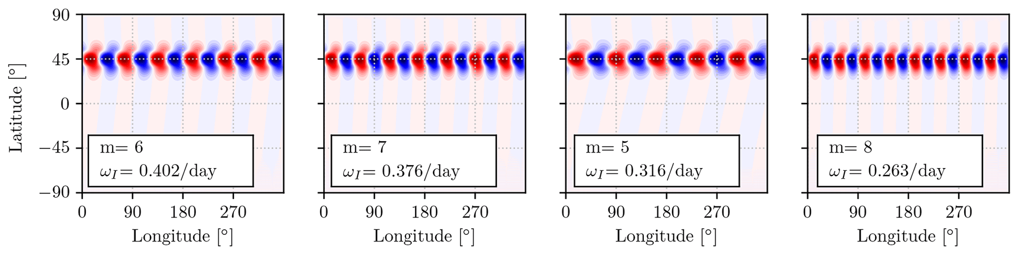
Figure 7The four most unstable modes from the linear analysis sorted according to their growth rate in the strong-jet case.
5.1 Extending the Wirth (2020) diagnostic
Determining a general definition of waveguidability and estimating it remain open research questions. A universal waveguidability metric should inform about the ability of Rossby waveguides to duct waviness and should be in principle applicable to any background flow. While developing such a metric is not the focus of the current study, we nonetheless need a metric that enables the comparison of background flows with jets at different latitudes. Here, we opt to consider the amount of enstrophy that remains at the forcing latitude compared to the global enstrophy. This implies a minimal change with respect to Wirth (2020), with an integration over all longitudes rather than just a sector. The normalized meridional enstrophy density E of a layer centered around φ=φ0 is here defined as
where Δφ=15° and is the square of the time-averaged vorticity anomaly from the background state. The time averaging operation is indicated by 〈⋅〉. It is important to consider that this definition requires a forcing centered around the same latitude where E is computed, φ0, as a source of vorticity. The so-defined metric E takes into account the enstrophy in the vicinity of the forcing, which will be high even in the absence of jet streams and thus cannot be directly used as a measure of the waveguidability. Within the definition (Eq. 19) the jet latitude φJ, forcing latitude φF, and latitude where the enstrophy anomaly is computed φ0 coincide with the same value: this enables the evaluation of the jet's capacity to hold the enstrophy (injected at the same latitude of the jet stream) within itself.
5.2 The single-jet case
With the help of the newly developed linear method, it is possible to efficiently estimate the equilibrium state for many jet velocities and jet latitudes and use it to calculate E for the linear simulations. This is shown in Fig. 8a for single jets with different jet latitudes and strengths. It is clear that the stronger the jet, the higher the normalized enstrophy density E, as noticed already for the jet at 45° N. However, when no jet is present (and therefore no waveguide should exist), E remains still high due to the enstrophy generated in the vicinity of the forcing. We also notice that E increases with latitude, as more enstrophy is found along the short latitude circles close to the pole.
In order to isolate just the contribution of the waveguide in keeping the energy at that latitude, Fig. 8b shows the difference ΔE between E(UJ, φ0) and E(0, φ0) (namely the normalized enstrophy density without any jet). Removing the contribution of solid-body rotation isolates the increase in E due to the presence of a waveguide. We see that ΔE increases with jet speed in a consistent way for all latitudes. An equatorial westerly jet (which is obviously not relevant to realistic situations) results in a weaker ΔE than in midlatitudes; this last result is presumably due to the fact that the Equator already constitutes a waveguide for a background solid-body rotation even without any jet superimposed.
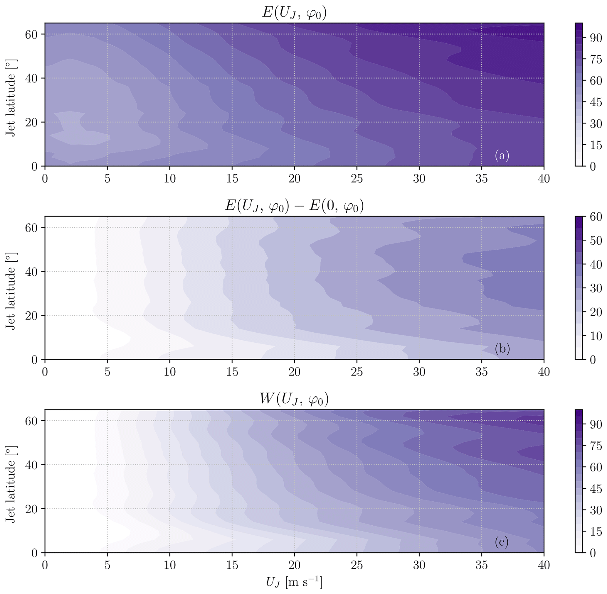
Figure 8(a) Normalized meridional enstrophy density of the single-jet zonal profiles (as in Eq. 17) for different jet latitudes and strengths, estimated according to Eq. (19) with φ0 equal to the jet latitude. The enstrophy field has been computed from the equilibrium state obtained from the linear method. Only narrow jets with σJ=5° have been considered. (b) Difference used to highlight the increment in normalized enstrophy density with the jet speed with respect to the solid-body case. (c) Estimated waveguidability calculated according to Eq. (20). All color scales are expressed in percent.
The increment ΔE due to the presence of the jet is, as expected, small for low jet speeds. However, ΔE remains below 50 % even for the high jet speed of 40 m s−1, for which one would expect values closer to 100 % (as in Wirth, 2020). This indicates that, even though useful to understand the relative waveguidability increase, ΔE would not make an appropriate universal waveguidability metric. In order to propose a simple assessment of the waveguidability property, one could consider how ΔE compares to an “ideal” waveguide at the same latitude, i.e., a waveguide that would keep all the enstrophy in the same latitude circle of the jet (E=1). This could be computed as the ratio
which is defined to be a number between 0 (no jet) and 1 (ideal waveguide). This ratio gives a direct measure of how the normalized enstrophy density is increased by the jet presence, relative to the increase achievable with an ideal waveguide. The so-defined waveguidability metric (Eq. 20) increases with jet speed from 0 % to around 90 %, as expected, but it also features an increase with latitude for strong jets (Fig. 8c). This trend of W with latitude is likely not due to the fact that high-latitude jets act as better waveguides than low-latitude jets because ΔE (i.e., the numerator of W) does not feature an analogous latitudinal variation. On the other hand, it likely results from the relative variation in E(0, φ0) with latitude visible in Fig. 8a, which leads to a reduction in the denominator of Eq. (20) at high latitudes. From a physical point of view, this means that a large part of the enstrophy is already kept at the latitude of the forcing even in the absence of a jet. For this reason, it is much easier to approach the status of “ideal waveguide” at high latitudes than at low latitudes, at least according to the W metric. This analysis also indicates that care is needed when estimating waveguidability, even in relatively simple single-jet configurations, as conclusions might be metric-dependent.
5.3 The double-jet case
After having considered the single-jet case, we now consider a configuration with two separate jets of width σJ=5° located at different latitudes. The double-jet setup was chosen as it is representative of the interplay between the subtropical and the eddy-driven jet streams observed in the Northern Hemisphere and because recent research has connected it to the occurrence of quasi-stationary Rossby waves and summer heat extremes (Rousi et al., 2022). The first jet is located at φJ=30° N and has a jet velocity of UJ=40 m s−1 (the associated perturbation field is shown in Fig. 9 for both the linear and nonlinear simulations). The second jet is located at φJ=60° N and also has a jet velocity of UJ=40 m s−1 (the associated perturbation field is shown in Fig. 10). A topographic forcing is imposed at the center of the latitudinal band where waveguidability is assessed using Eq. (20).
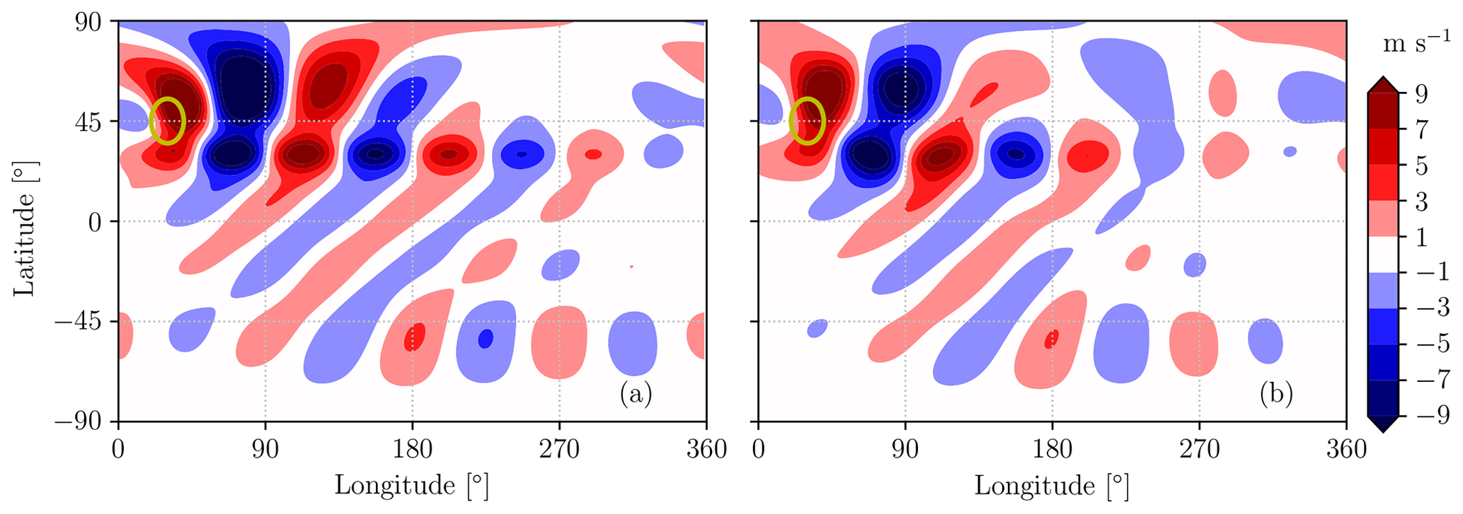
Figure 9Meridional velocity associated with a zonal jet characterized by UJ=40 m s−1 with φJ=30° N at the equilibrium state from the linear analysis (a) and averaged between 10 and 100 d from the simulation start with the nonlinear solver (b).
The perturbations resulting from the 30° N jet feature a combination of great-circle and along-jet propagation that is properly represented by both the linear and nonlinear approaches (Fig. 9). On the other hand, for the jet at 60° N the along-jet propagation is obtained only in the linear simulation, while it is much weaker in the nonlinear simulation (Fig. 10). The weakening of along-jet propagation can be due to an enhanced equatorward propagation of the stationary wave in the nonlinear case, given that the forcing is located at 45° N, possibly combined with enhanced dissipation. By using Eq. (20), the waveguidability of the 30° N jet (calculated from the linear simulations and at the jet latitude) is 84 %, while the one of the 60° N jet is 92 %, highlighting that jets with the same velocity but different latitudes act as similarly efficient waveguides.
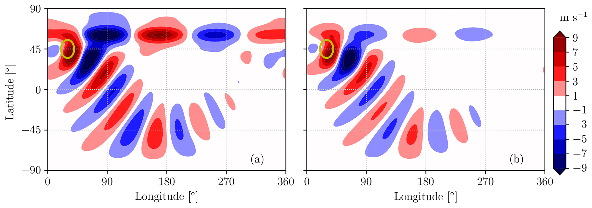
Figure 10Meridional velocity associated with a zonal jet characterized by UJ=40 m s−1 with φJ=60° N at the equilibrium state from the linear analysis (a) and averaged between 10 and 100 d from the simulation start with the nonlinear solver (b).
Moving to the double-jet configuration we notice, first of all, a good agreement between the linear and the nonlinear solution (Fig. 11). Rossby wave propagation occurs separately along the waveguides delineated by the two jet streams, while great-circle propagation to the Southern Hemisphere is smaller in the double-jet configuration than for the jets taken individually. The double-jet pattern corresponds roughly to the combination of the patterns of the linear solutions for the two individual jets. However, this is not true for the nonlinear solutions because of the previously discussed lack of Rossby wave propagation along the 60° N jet in the nonlinear single-jet case. It might be that forced meridional velocity perturbations along the 30° N jet stream could provide energy to the jet at 60° N, which would otherwise be attenuated as in the single-jet case (Fig. 10b); however, this hypothesis would need further verification. Furthermore, the waveguidability of the two jets is lower than the one of the two distinct jets: the 30° N jet has a value of the waveguidability metric of 70 %, while the 60° N jet has a value of 82 %. The waveguidability of the 60° N jet has been estimated using Eq. (20), considering a fictitious forcing centered at 60° N and by monitoring the enstrophy anomaly around the same latitude (and similarly for the 30° N jet). The fact that the waveguidability is reduced compared to the isolated jet case by 10 % for both jets is probably due to the jet streams' ability to attract leaked enstrophy from the surrounding regions (including the other jet stream), making the two jets more leaky than the ideal waveguides. However, the reader is warned that these results are likely sensitive to the choice of the reference state in Eq. (20) (here taken as the solid-body background flow).
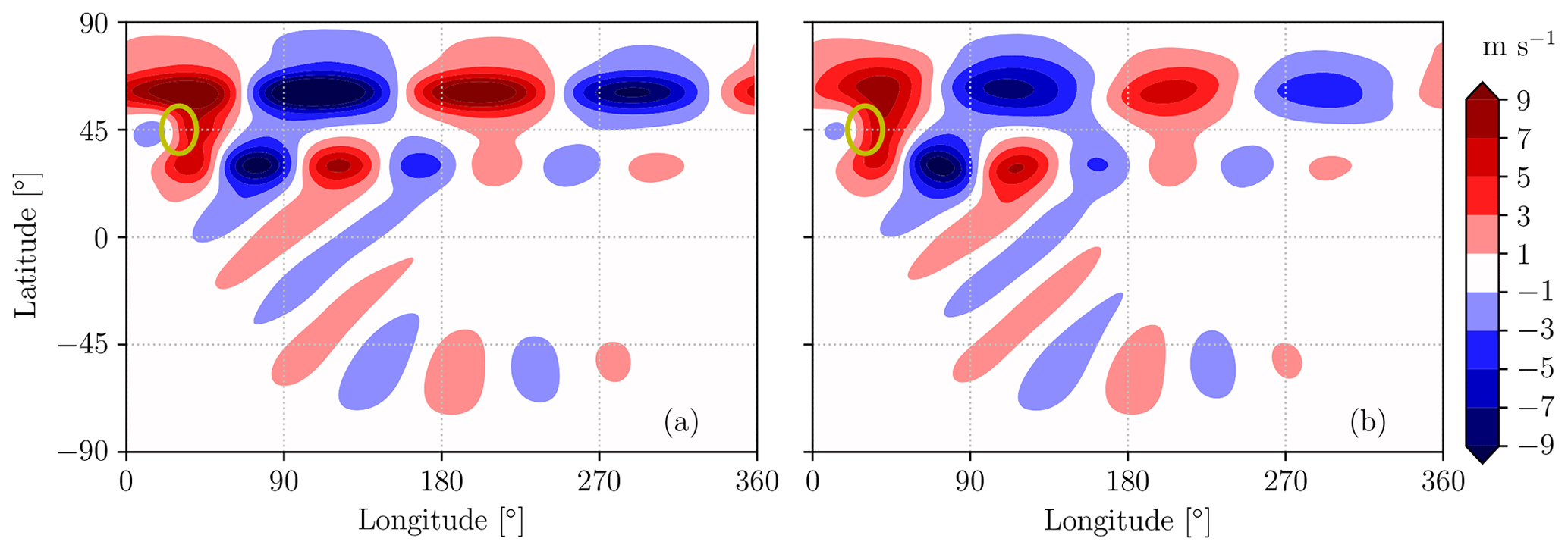
Figure 11Meridional velocity associated with two zonal jets ( m s−1 with N and m s−1 with N) at the equilibrium state from the linear analysis (a) and averaged between 10 and 100 d from the simulation start with the nonlinear solver (b).
Even though the basic physical concepts behind Rossby wave propagation have been known for several decades, we are still far from a general comprehension of Rossby wave evolution in non-idealized flow setups, such as the ones typically associated with extreme weather events. The understanding of Rossby wave propagation along the waveguide provided by the upper-level jet stream, in particular, remains challenging. This work revisited the problem of Rossby wave propagation in a non-divergent, barotropic flow on a sphere, following the specification of a zonally symmetric background flow. Such a simplified setup allowed us to advance the state of the art, both in terms of model and process understanding.
We described a novel, linearized mathematical treatment of the barotropic Rossby wave propagation problem that allows one to efficiently obtain the steady-state Rossby wave response to a given topographic forcing. The approach relies on the framing of the barotropic vorticity equation on the sphere as an eigenvalue problem. Here, the eigenfunctions represent the flow response to the topographic forcing in the meridional direction only (as the background flow is zonally symmetric and a Fourier series decomposition is applied in the zonal direction), while the sign of the eigenvalues' imaginary part (the growth rate) allows one to determine the stability of the eigenfunctions, with a positive value indicating linear instability and exponential growth of the mode when triggered. In distinct contrast to ray-tracing theory, the present approach has general validity for any background flow and forcing combination, does not require projecting the flow field on a Mercator plane, and does not assume any scale separation between the background flow and the waves.
Some features of Rossby waves occurring in the barotropic model have been elucidated, in particular for the onset and the evolution of transient Rossby waves that, under some circumstances, accompany the steady-state response. Such waves are the result of a barotropic instability arising at high jet speed, when the growth rate actually turns positive. The change in sign in the absolute vorticity gradient (i.e., the Rayleigh criterion in the non-dissipative case) is not immediately associated with the onset of barotropic instability, which was observed at higher jet speeds. This happens because dissipation shifts the linear neutral curve towards higher velocities. Even more intriguing, nonlinear simulations showed signs of barotropic instability further beyond the linear neutral curve, pointing to potential damping effects operated by nonlinear terms (e.g., wave–wave and wave–mean-flow interactions). This dynamic was further investigated by means of empirical orthogonal functions, which showed that modes with an azimuthal wavenumber of 5 up to 7 are associated with traveling waves of fixed amplitude, a dynamic originated by nonlinear effects. Nevertheless, the averaged flow field in the nonlinear simulation resembles the unstable equilibrium state calculated from the linear method. The latter is an equilibrium state obtained by removing the time derivative and is therefore an approximation of the equilibrium condition of the nonlinear system, too.
By means of the linearized analysis we revisited the waveguidability problem for a variety of background flow configurations. A new metric of waveguidability, based on a time average of the enstrophy anomaly, has been proposed to compare jet streams located at different latitudes. We reconfirmed earlier results and noticed that, in a barotropic framework, jet waveguidability is strongly related to jet speed, while jet latitude plays a considerably smaller role. The application of the proposed approach to a double-jet configuration showed that (a) the equatorward propagation of Rossby waves is weakened in a double-jet case compared to the no-jet case, (b) the double-jet response roughly corresponds to the linear combination of the individual jet responses, although (c) the waveguidability of each jet taken individually seems to be higher than when the two jets occur in a double-jet configuration. These results extend the analysis by Wirth (2020) and pave the way for a more targeted analysis of Rossby wave propagation in the presence of multiple jets, together with the development of appropriate metrics to quantify waveguidability in such circumstances.
We envisage several future applications of our analysis approach, for example, a systematic waveguidability assessment for different forcings and background zonal wind profiles, including a detailed investigation of double-jet configurations. Another relevant application would be to understand the role of orography in forcing Rossby waves with specific zonal wavenumbers, as amplified waves of specific wavenumbers have been related to surface weather extremes during summer (as noticed, among others, by Coumou et al., 2014; Jiménez-Esteve et al., 2022). Although we do not attempt this here, this evidence could enable building a reduced-order model of a barotropic atmosphere where the spatial modes are provided by the equilibrium state and by the most unstable modes (this information being retrieved exclusively from the linear analysis), while the temporal coefficients could be determined by solving a small set of nonlinear ordinary differential equations (Holmes et al., 2012).
In conclusion, we present a relatively simple and computationally efficient way to study the steady and unsteady Rossby wave response to topography in a variety of idealized background flow configurations. This approach goes beyond a number of limitations of ray-tracing theory for determining waveguidability, and we have illustrated the physical insights it can provide by considering a wide parameter sweep of jet speeds and latitudes and a double-jet configuration.
Equation (11) introduces the Laplace operator ℒ in the transformed space together with the boundary conditions needed to avoid the pole singularity:
and similarly for θ=π. Consequently, there are two boundary conditions for |m|≤1 and four otherwise. An additional boundary condition must be introduced at m=0 as in order to set the value of the streamfunction at one pole since, otherwise, the streamfunction would be defined up to an additive constant, making the numerical problem singular.
Following Peyret (2002), the solution of Eq. (10) is calculated by a spectral collocation method in terms of orthogonal polynomials. In the present work, Chebyshev polynomials, Tq(θ), and the decomposition
are used. The N+1 collocation points are described by a shifted Gauss–Lobatto distribution:
implying a refinement of the colatitude distribution near the poles. This is in contrast to the Legendre and associated Legendre polynomials that account for a more appropriate resolution at the poles. Nevertheless, Chebyshev polynomials have been preferred here since an exact method to calculate the spectral coefficients exists for them, while the Legendre polynomials require a numerical quadrature scheme (Krishnamurti et al., 2006). The choice of the specific family of polynomials influences only the derivatives in the meridional direction and the meridional discretization, while the zonal discretization is still based on the Fourier transform, as is the case for spherical harmonics.
Rather than working with the spectral coefficients, aq(t; m), here it is preferred to work directly with the value of the streamfunction at the collocation points, , as unknowns collected into a vector, significantly facilitating the interpretation of the results. The derivatives of the streamfunction are calculated as
where the matrices D(1) and D(2) provide the first- and second-order derivatives (Peyret, 2002). Another advantage of the Chebyshev basis is that the matrices D(1) and D(2) are analytically known (Peyret, 2002; Canuto et al., 2006), although some modifications to limit the effect of round-off errors have been implemented (Bayliss et al., 1995).
By exploiting Eq. (A4), the discretized Laplace operator becomes
where I indicates the identity matrix. This implies that the Laplace operator becomes a numerical matrix since the spatial dependence of the variables is provided by the Fourier modes (in the zonal direction) and by the Chebyshev polynomials (in the meridional direction). Once the Laplace operator has been discretized, the matrices A and B in Eq. (12) are obtained from their definition.
As stated in Eq. (A1), the boundary conditions at the poles have been imposed by removing two, three or four points from the analysis so that the size of the matrices A or B is for m=0, for |m|=1 and otherwise. This has the advantage that the reduced forms of A and B are just related to the dynamics of the modeled system rather than the boundary conditions (the reader is referred to Sect. 3.7.1 of Peyret, 2002, for a detailed description of how the matrices can be reduced), together with a decrease in the computational cost.
If B is nonsingular, it is possible to perform the eigendecomposition , where the columns of P are the eigenvectors and Λ is a diagonal eigenvalue matrix. The analytical solution of Eq. (12) is found to be
with indicating the initial condition of the streamfunction. In the special case of a steady forcing, Eq. (A6) becomes
The first term of Eqs. (A6) and (A7) is the homogeneous unforced solution of the linear system with initial condition , while the second term is the forced solution with zero initial condition.
Since the eigenvalues, Λ, and eigenfunctions, P, depend on the zonal velocity, U; Rossby number, Ro; and wavenumber, m, they are calculated and stored for all the considered wavenumbers for a given zonal velocity profile and Rossby number. Since they do not depend on the actual forcing applied, once they are computed they can be used with any kind of forcing according to Eqs. (A6)–(A7). Furthermore, since the equation is linear, no aliasing instability is present and each eigenmode does not interact with the others. Equation (A6) enables the calculation of the solution at any time without the need for numerical integration. This is nevertheless necessary if the forcing is time dependent, although with a definite integral instead.
The code can be downloaded from GitHub (https://github.com/AntSegalini/barotropic_instability_Chebyshev, last access: 4 August 2024) with the DOI https://doi.org/10.5281/zenodo.13215495 (Segalini, 2024).
The simulation results are available upon request to the authors.
AS developed the theory, performed the simulations shown in the paper and analyzed the data. All authors contributed equally to the interpretation of the results. AS and JR prepared the manuscript, assisted by GM and VW for review and editing.
The contact author has declared that none of the authors has any competing interests.
Publisher’s note: Copernicus Publications remains neutral with regard to jurisdictional claims made in the text, published maps, institutional affiliations, or any other geographical representation in this paper. While Copernicus Publications makes every effort to include appropriate place names, the final responsibility lies with the authors.
The authors are thankful to Camille Li and the two anonymous reviewers for very insightful comments during the revision process.
This research has been supported by the European Research Council (ERC) under the European Union’s Horizon 2020 research and innovation program (grant no. 948309, CENÆ project, PI: Gabriele Messori) and by the Swiss National Science Foundation (SNSF) (grant no. PZ00P2_209135).
This paper was edited by Camille Li and reviewed by two anonymous referees.
Ambrizzi, T., Hoskins, B. J., and Hsu, H.-H.: Rossby Wave Propagation and Teleconnection Patterns in the Austral Winter, J. Atmos. Sci., 52, 3661–3672, https://doi.org/10.1175/1520-0469(1995)052<3661:RWPATP>2.0.CO;2, 1995. a
Baldauf, M. and Brdar, S.: An analytic solution for linear gravity waves in a channel as a test for numerical models using the non-hydrostatic, compressible Euler equations, Q. J. Roy. Meteor. Soc., 139, 1977–1989, https://doi.org/10.1002/qj.2105, 2013. a
Bayliss, A., Class, A., and Matkowsky, B. J.: Roundoff error in computing derivatives using the Chebyshev differentiation matrix, J. Comput. Phys., 116, 380–383, 1995. a
Boyd, J. P.: The Effects of Latitudinal Shear on Equatorial Waves. Past I: Theory and Methods, J. Atmos. Sci., 35, 2236–2258, https://doi.org/10.1175/1520-0469(1978)035<2236:TEOLSO>2.0.CO;2, 1978. a
Branstator, G.: Circumglobal teleconnections, the jet stream Waveguide, and the North Atlantic Oscillation, J. Climate, 15, 1893–1910, https://doi.org/10.1175/1520-0442(2002)015<1893:CTTJSW>2.0.CO;2, 2002. a
Brayshaw, D. J., Hoskins, B., and Blackburn, M.: The basic ingredients of the North Atlantic Storm Track. Part I: Land–Sea contrast and orography, J. Atmos. Sci., 66, 2539–2558, https://doi.org/10.1175/2009JAS3078.1, 2009. a
Campbell, L. and Maslowe, S.: Forced Rossby wave packets in barotropic shear flows with critical layers, Dynam. Atmos. Oceans, 28, 9–37, https://doi.org/10.1016/S0377-0265(98)00044-X, 1998. a
Canuto, C., Hussaini, M. Y., Quarteroni, A., and Zang, T. A.: Spectral methods. Fundamentals in single domains, Sci. Comput., Berlin, Springer, ISBN 3-540-30725-7, https://doi.org/10.1007/978-3-540-30726-6, 2006. a, b
Coumou, D., Petoukhov, V., Rahmstorf, S., Petri, S., and Schellnhuber, H. J.: Quasi-resonant circulation regimes and hemispheric synchronization of extreme weather in boreal summer, P. Nat. Acad. Sci. USA, 111, 12331–12336, https://doi.org/10.1073/pnas.1412797111, 2014. a, b, c
Davies, H.: Weather chains during the 2013/2014 winter and their significance for seasonal prediction, Nat. Geosci., 8, 833–837, https://doi.org/10.1038/ngeo2561, 2015. a
Di Capua, G., Sparrow, S., Kornhuber, K., Rousi, E., Osprey, S., Wallom, D., van den Hurk, B., and Coumou, D.: Drivers behind the summer 2010 wave train leading to Russian heatwave and Pakistan flooding, npj Climate and Atmospheric Science, 4, 1–14, 2021. a
Garcia, R. R. and Salby, M. L.: Transient response to localized episodic heating in the tropics. Part II: Far-field behavior, J. Atmos. Sci., 44, 499–532, 1987. a
Garfinkel, C. I., White, I., Gerber, E. P., Jucker, M., and Erez, M.: The building blocks of Northern Hemisphere wintertime stationary waves, J. Climate, 33, 5611–5633, https://doi.org/10.1175/JCLI-D-19-0181.1, 2020. a
Gill, A. E.: Atmosphere-ocean dynamics, vol. 30, Academic Press, ISBN-13 978-0-12-283520-9, 1982. a
Harnik, N., Messori, G., Caballero, R., and Feldstein, S. B.: The Circumglobal North American wave pattern and its relation to cold events in eastern North America, Geophys. Res. Lett., 43, 11015–11023, https://doi.org/10.1002/2016GL070760, 2016. a
Haurwitz, B.: The motion of atmospheric disturbances on the spherical earth, J. Mar. Res., 3, 254–267, 1940. a
Held, I. M.: Stationary and quasi-stationary eddies in the extratropical troposphere: Theory, in: Large-Scale Dynamical Processes in the Atmosphere, edited by: Hoskins, B. J. and Pearce, R. P., Academic Press, 127–168, ISBN-13 978-0123566805, 1983. a
Held, I. M., Ting, M., and Wang, H.: Northern Winter Stationary Waves: Theory and Modeling, J. Climate, 15, 2125–2144, https://doi.org/10.1175/1520-0442(2002)015<2125:NWSWTA>2.0.CO;2, 2002. a
Holmes, P., Lumley, J. L., Berkooz, G., and Rowley, C. W.: Turbulence, coherent structures, dynamical systems and symmetry, Cambridge University Press, ISBN-13 978-1107008250, 2012. a
Hoskins, B. J. and Ambrizzi, T.: Rossby Wave Propagation on a realistic longitudinally varying flow, J. Atmos. Sci., 50, 1661–1671, https://doi.org/10.1175/1520-0469(1993)050<1661:RWPOAR>2.0.CO;2, 1993. a, b
Hoskins, B. J. and Karoly, D. J.: The steady linear response of a spherical atmosphere to thermal and orographic Forcing, J. Atmos. Sci., 38, 1179–1196, https://doi.org/10.1175/1520-0469(1981)038<1179:TSLROA>2.0.CO;2, 1981. a, b, c, d
Hoskins, B. J. and Valdes, P. J.: On the existence of Storm-Tracks, J. Atmos. Sci., 47, 1854–1864, https://doi.org/10.1175/1520-0469(1990)047<1854:OTEOST>2.0.CO;2, 1990. a
Hou, A. Y. and Farrell, B. F.: Excitation of nearly steady finite-amplitude barotropic waves, J. Atmos. Sci., 43, 720–728, 1986. a
Jiménez-Esteve, B., Kornhuber, K., and Domeisen, D. I. V.: Heat Extremes Driven by Amplification of Phase-Locked Circumglobal Waves Forced by Topography in an Idealized Atmospheric Model, Geophys. Res. Lett., 49, e2021GL096337, https://doi.org/10.1029/2021GL096337, 2022. a, b
Joly, A. and Thorpe, A. J.: Frontal instability generated by tropospheric potential vorticity anomalies, Q. J. Roy. Meteor. Soc., 116, 525–560, https://doi.org/10.1002/qj.49711649302, 1990. a
Kalnay, E.: Atmospheric modeling, data assimilation and predictability, Cambridge University Press, ISBN-13 978-0521796293, 2003. a
Kornhuber, K. and Messori, G.: Recent increase in a recurrent pan-Atlantic wave pattern driving concurrent wintertime extremes, B. Am. Meteorol. Soc., 104, E1694–E1708, 2023. a
Kornhuber, K., Osprey, S., Coumou, D., Petri, S., Petoukhov, V., Rahmstorf, S., and Gray, L.: Extreme weather events in early summer 2018 connected by a recurrent hemispheric wave-7 pattern, Environ. Res. Lett., 14, 054002, https://doi.org/10.1088/1748-9326/ab13bf, 2019. a
Krishnamurti, T. N., Bedi, H., Hardiker, V., and Watson-Ramaswamy, L.: An introduction to global spectral modeling, vol. 35, Springer Science and Business Media, ISBN-13 978-0195094732, 2006. a
Kuo, H.-l.: Dynamic instability of two-dimensional nondivergent flow in a barotropic atmosphere, J. Atmos. Sci., 6, 105–122, 1949. a
Lachmy, O. and Harnik, N.: Wave and jet maintenance in different flow regimes, J. Atmos. Sci., 73, 2465–2484, 2016. a
Leutwyler, D. and Schär, C.: Barotropic Instability of a Cyclone Core at Kilometer-Scale Resolution, J. Adv. Model. Earth Sy., 11, 3390–3402, https://doi.org/10.1029/2019MS001847, 2019. a
Manola, I., Selten, F., de Vries, H., and Hazeleger, W.: “Waveguidability” of idealized jets, J. Geophys. Res.-Atmos., 118, 10432–10440, https://doi.org/10.1002/jgrd.50758, 2013. a
Martius, O., Schwierz, C., and Davies, H. C.: Tropopause-Level Waveguides, J. Atmos. Sci., 67, 866–879, https://doi.org/10.1175/2009JAS2995.1, 2010. a
Martius, O., Wehrli, K., and Rohrer, M.: Local and remote atmospheric Responses to Soil Moisture Anomalies in Australia, J. Climate, 34, 9115–9131, https://doi.org/10.1175/JCLI-D-21-0130.1, 2021. a
Petoukhov, V., Rahmstorf, S., Petri, S., and Schellnhuber, H. J.: Quasiresonant amplification of planetary waves and recent Northern Hemisphere weather extremes, P. Natl. Acad. Sci. USA, 110, 5336–5341, https://doi.org/10.1073/pnas.1222000110, 2013. a
Peyret, R.: Spectral methods for incompressible viscous flow, vol. 148, New York, NY, Springer, ISBN 0-387-95221-7, 2002. a, b, c, d, e
Rhines, P. B.: Waves and turbulence on a beta-plane, J. Fluid Mech., 69, 417–443, 1975. a
Rossby, C.-G.: Relation between variations in the intensity of the zonal circulation of the atmosphere and the displacements of the semi-permanent centers of action, J. Mar. Res., 2, 38–55, 1939. a
Rossby, C.-G.: Planetary flow patterns in the atmosphere, Q. J. Roy. Meteor. Soc., 66, 68–87, 1940. a
Rousi, E., Kornhuber, K., Beobide-Arsuaga, G., Luo, F., and Coumou, D.: Accelerated western European heatwave trends linked to more-persistent double jets over Eurasia, Nat. Commun., 13, 1–11, 2022. a, b, c
Schaeffer, N.: Efficient spherical harmonic transforms aimed at pseudospectral numerical simulations, Geochem. Geophy. Geosy., 14, 751–758, https://doi.org/10.1002/ggge.20071, 2013. a
Segalini, A.: AntSegalini/barotropic_instability_Chebyshev: Barotropic stability code (v0.0), Zenodo [code], https://doi.org/10.5281/zenodo.13215495, 2024. a
Teng, H. and Branstator, G.: Amplification of waveguide teleconnections in the Boreal summer, Curr. Clim. Change Rep., 5, 421–432, https://doi.org/10.1007/s40641-019-00150-x, 2019. a
White, R. H., Kornhuber, K., Martius, O., and Wirth, V.: From atmospheric waves to heatwaves: A waveguide perspective for understanding and predicting concurrent, persistent and extreme extratropical weather, B. Am. Meteorol. Soc., 103, E923–E935, https://doi.org/10.1175/BAMS-D-21-0170.1, 2022. a, b
Wirth, V.: Waveguidability of idealized midlatitude jets and the limitations of ray tracing theory, Weather Clim. Dynam., 1, 111–125, https://doi.org/10.5194/wcd-1-111-2020, 2020. a, b, c, d, e, f, g, h, i, j, k, l, m, n, o, p
Wirth, V. and Polster, C.: The problem of diagnosing jet waveguidability in the presence of large-amplitude eddies, J. Atmos. Sci., 78, 3137–3151, https://doi.org/10.1175/JAS-D-20-0292.1, 2021. a, b
Wirth, V., Riemer, M., Chang, E. K. M., and Martius, O.: Rossby wave packets on the midlatitude waveguide – A review, Mon. Weather Rev., 146, 1965–2001, https://doi.org/10.1175/MWR-D-16-0483.1, 2018. a, b
Yang, G.-Y. and Hoskins, B. J.: Propagation of Rossby waves of nonzero frequency, J. Atmos. Sci., 53, 2365–2378, 1996. a
- Abstract
- Introduction
- Model framework and numerical details
- Model setup and validation
- Single-jet configuration: stability and dynamics
- Waveguidability assessment
- Conclusions
- Appendix A: Spectral solution of the barotropic vorticity equation
- Code availability
- Data availability
- Author contributions
- Competing interests
- Disclaimer
- Acknowledgements
- Financial support
- Review statement
- References