Clear-air turbulence derived from in situ aircraft observation – a weather feature-based typology using ERA5 reanalysis

Clear-air turbulence (CAT) endangers aviation safety and early understanding of the phenomenon was obtained mainly by analysing the corresponding synoptic weather situation. In this study, the relationship between CAT and different synoptic weather features is revisited based on in situ eddy dissipation rate measurements by commercial aircraft and modern reanalysis data (ERA5 reanalysis). In the years from 2019 to 2022, 4880 moderate-or-greater turbulence events are identified in predominantly clear-air conditions in the Northern Hemisphere. Most of the events identified occur over the contiguous U.S. and along the major flight corridors in the North Atlantic and western North Pacific. They are associated frequently with potential vorticity (PV) streamers, which are used as a proxy for Rossby wave breaking (RWB), and/or warm conveyor belt (WCB) ascents at the event locations. Events which are concurrent with RWB in the absence of WCB ascents are classified as type I. They constitute around 40 % of the events and are found evenly across the contiguous U.S. Events which are concurrent with WCB ascents are classified as type II. They account for around 30 % of the events and are more concentrated over the eastern U.S. and the East China Sea. Analysing the environmental conditions associated with the events, higher values of horizontal deformation are found on average in the vicinity of type I events, and the high horizontal deformation associated with RWB is considered as the possible cause of this type of CAT. Type II events occur more frequently in the presence of negative PV, together with higher averaged cloud ice water content and wind speed. The presence of negative PV, which is most likely due to diabatic PV reduction in clouds, may indicate that inertial or symmetric instabilities or enhanced local wind shear due to the strengthened outflow from WCBs are possible causes of CAT for type II events. The suggested linkages are further supported by examining the ERA5 grid point data. When grid points with high horizontal deformation are examined, they are mostly found in RWB regions and show an enhanced chance of turbulence. This collocation of RWB, high horizontal deformation, and turbulence is particularly prominent over the Western U.S. Similarly, grid points with negative PV values also show a higher probability of turbulence and a noteworthy fraction is collocated with WCB ascents. The results thus (i) reveal the important roles of RWB and WCB ascents for CAT, (ii) provide a better explanation of the physical mechanisms triggering CAT in the presence of RWB and WCB ascents, and (iii) highlight the importance of in situ observations for deepening the understanding of CAT. Furthermore, the weather-feature perspective employed in this study may also provide insights to interpret the climatology of CAT or projected changes of CAT in the future.

1 Introduction

Turbulence in the upper troposphere and lower stratosphere (UTLS) poses threats to aviation safety at cruising altitudes. In particular, clear-air turbulence (CAT), which occurs outside of convective clouds, is difficult for pilots to detect onboard and challenging for numerical weather prediction models to capture. CAT has therefore continuously been a challenging research topic, with the hope that a better understanding of the phenomenon can yield more accurate forecasts, which ultimately help pilots avoid unexpected turbulence.

In the pioneering studies on CAT, researchers analysed dozens of reports by research and commercial aircraft to identify the favourable meteorological conditions for the occurrence of CAT (e.g. Hislop, 1951; Bannon, 1952). The conclusion that CAT is frequently observed in regions with high vertical wind shear (Hislop, 1951) and in the vicinity of the upper-level jet streams (Bannon, 1952) points towards the important role of wind shear in the generation of CAT. The relevance of Kelvin–Helmholtz instability (KHI), which is also referred to as shear instability in a stably stratified fluid, has since been recognised as a source of CAT (e.g. Reiter, 1969; Dutton and Panofsky, 1970). The gradient Richardson number Ri, which is the ratio of the stabilising force due to stratification to the destabilising force due to shear, is commonly used as a diagnostic for identifying potential regions of KHI, where a low value of Ri indicates a high likelihood of CAT (e.g. Hislop, 1951; Bannon, 1951), though the strength of this correlation was found to vary seasonally and geographically (Rustenbeck, 1963). The upper-level jet stream was hence the earliest mentioned weather feature linked to CAT as it can create regions with enhanced vertical shear and low values of Ri.

Subsequent studies revealed that the likelihood of CAT varies along the jet stream (e.g. Chambers, 1955) and the preferential locations of CAT occurrence in different upper-level flow situations were examined by analysing all observations available. For instance, CAT encounters are found in regions with strong horizontal shear associated with cyclonically and anticyclonically curved jet streams (Endlich, 1964), confluent zones between jet streams (Reiter and Nania, 1964), and diffluent and confluent zones associated with upper-low formation (Hopkins, 1977). The direction and location of the jet core relative to topography and surface cyclogenesis were also analysed to investigate their influence on CAT (Hopkins, 1977). Moreover, the CAT locations were documented relative to flow features including the jet axes, ridges, troughs, and upper-lows. These relationships connecting CAT and synoptic-scale features then informed the guidelines for CAT forecasting since the 1970s (e.g. Hopkins, 1977; Lee et al., 1984), profiting from the upper-air observation network and numerical weather forecasts being capable of diagnosing and predicting the evolution of synoptic weather systems.

With spatially denser meteorological observations and improved resolution of numerical weather forecasting models, it became possible to search for statistical and physical relationships for CAT with its associated mesoscale environment. One approach was to correlate numerous observations with different physical quantities describing the environmental conditions and study the potential underlying physical processes that cause these high correlations. Vertical wind shear and horizontal deformation were repeatedly found to be quantities highly correlated with CAT (e.g. Mancuso and Endlich, 1966) and the product of the two is the foundation of one of the widely adopted turbulence indices (Ellrod and Knapp, 1992) in CAT forecasting. While vertical wind shear is readily related to KHI, different interpretations of the role of horizontal deformation exist (e.g. Mancuso and Endlich, 1966; Ellrod and Knapp, 1992). Several other semi-empirical indices were also developed based on flow curvature, shear, and environmental Richardson number (e.g. Roach, 1970; Brown, 1973).

Apart from the empirically or statistically developed turbulence diagnostics or indicators, some others were also introduced through theoretical consideration and case studies. For instance, the presence of inertial instability, which is indicated by negative absolute vorticity or potential vorticity (PV) (Schultz and Schumacher, 1999), was suggested to be a possible mechanism for CAT occurrence (Knox, 1997). This wide range of turbulence diagnostics laid the foundation of modern automated turbulence forecasts from numerical weather predictions, including the Graphical Turbulence Guidance (Sharman et al., 2006), which is a weighted sum of a selected set of diagnostics. While the employment of turbulence diagnostics has been proven useful in CAT forecasting and helped reveal the possible mesoscale mechanism associated with CAT occurrence, the focus on these diagnostics obscures the linkage of CAT to the synoptic weather feature to some extent, as they are all point measures and do not consider the synoptic flow patterns.

The exploration of other possible mechanisms of CAT occurrence and the associated meteorological situations was complemented by elaborate case studies. High-resolution numerical simulations showed that gravity waves initiated in the upper-level jet-front system can lead to the occurrence of CAT (e.g. Lane et al., 2004; Koch et al., 2005). Other case studies also investigated CAT occurrence in tropopause folds (e.g. Lee and Chun, 2018; Rodriguez Imazio et al., 2022), a feature closely related to the upper-level jet-front system. Apart from dry dynamical processes like gravity waves and tropopause folding, the role of moist processes in causing CAT outbreaks is clearly demonstrated in various recent simulation studies (e.g. Trier et al., 2012; Trier and Sharman, 2016; Trier et al., 2020, 2022), in which gravity waves induced by convection or enhanced shear due to convective outflow are shown to be conducive to CAT occurrence. Though case studies enable detailed analysis of the dynamic processes leading to CAT occurrence, how often the studied situation causes CAT encounters by aircraft remains unclear.

Moreover, despite the extensive studies conducted targeting the relationships between CAT and various weather features, the list is most likely incomplete, especially when considering the advanced understanding of different weather systems. For instance, the contribution of Rossby wave breaking (RWB) to turbulence outbreak was listed as a research need by Sharman et al. (2016). In the extratropical tropopause region, synoptic-scale RWB is found in the nonlinear, final phase of the baroclinic wave cycle (Martius and Rivière, 2016) and manifested as filament-like features in the PV field, often referred to as PV streamers (Wernli and Sprenger, 2007). It is then natural to query if the nonlinear formation and breakup of PV streamers promote CAT occurrence. In addition, warm conveyor belts (WCB) (Browning et al., 1973), which are coherent ascending airstreams in extratropical cyclones, can generate negative PV near the tropopause by the embedded convection (e.g. Oertel et al., 2020; Harvey et al., 2020). The presence of inertial or symmetric instability in the tropopause region (which requires negative PV values) together with the previously documented importance of moist processes in triggering CAT hence provoke the question of whether CAT occurrence is favoured in the vicinity of WCBs.

Therefore, revisiting the topic of synoptic weather features and CAT is needed and this is further facilitated by the advancement in CAT observation and meteorological data. In the past, studies based on CAT observations (e.g. Sharman et al., 2006; Wolff and Sharman, 2008) mostly relied on pilot reports, which contain uncertainties in turbulence intensity, location, and time (Schwartz, 1996). Automated in situ measurements of the cubic root of the eddy dissipation rate (EDR), which indicates turbulence intensity in the atmosphere, have been introduced to commercial aircraft in recent years (Sharman et al., 2014). This measure is aircraft-independent and provides an increased amount of objective turbulence observations. Also, the continuous improvement in numerical weather prediction models enabled the production of reanalysis data with higher spatial and temporal resolution (e.g. Hersbach et al., 2020), allowing a better characterisation of the meteorological environment associated with CAT. A more systematic and comprehensive analysis of the relationship between different synoptic weather features and CAT is hence possible.

In this study, we employ in situ EDR measurements from commercial aircraft together with a weather feature database based on reanalysis data to address the following research questions:

• Which synoptic weather features that affect the tropopause region, are typically found in the neighbourhood of the observed CAT events?

• What are the characteristics of the environmental conditions associated with these weather-feature concurrent CAT events?

• Where are these weather-feature concurrent CAT events usually observed?

• What are the potential generating mechanisms for these weather-feature concurrent CAT events?

The description of the data and method will be presented in Sect. 2, followed by the results of the analysis in Sect. 3. Further discussion on the results and their implications will be given in Sect. 4 and the major conclusions will be summarised in Sect. 5.

2 Data and methods

2.1 Meteorological data and weather features

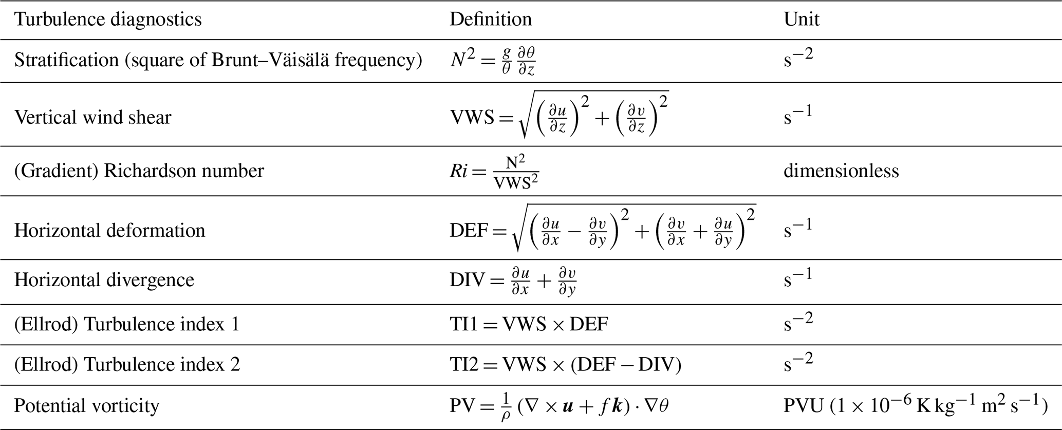
The ERA5 reanalysis data (Hersbach et al., 2020) from the European Centre for Medium-Range Weather Forecasts (ECMWF) are used to analyse the synoptic environment associated with the observed CAT events. The meteorological fields are available hourly and are retrieved at a horizontal resolution of 0.5° on a regular latitude-longitude grid on the model sigma-hybrid levels. Turbulence diagnostics are also computed from the reanalysis data on this grid and are listed in Table 1.

Table 1 Definition of grid point turbulence diagnostics based on ERA5, where u = $(u,v,w)$ is the wind vector, g is the acceleration due to gravity, f is the Coriolis parameter, ρ is the air density, and θ is the potential temperature.

In addition, a set of weather features observed in the mid-latitude UTLS region has been identified from the ERA5 reanalysis data with methods documented in Sprenger et al. (2017). This weather feature database facilitates the examination of the linkages between different weather systems and CAT in the UTLS region. Weather features presented in this study include upper-level jet streams, PV streamers (as a proxy for RWB), warm conveyor belts (WCBs), with some others (e.g. surface extratropical cyclones, anticyclones, tropopause folds) being explored but not being further discussed. All features examined are first identified in the reanalysis and converted into a corresponding two-dimensional mask (similar to the common land-sea mask), which is referred to as the “weather feature mask”, with value 1 indicating its presence and 0 indicating its absence.

The definitions of the three weather features which will be discussed in this study are outlined here. The upper-level jet streams are defined as regions with the vertically averaged horizontal wind speed from 500 to 100 hPa being higher than 30 m s⁻¹ (Koch et al., 2006). The PV streamers are defined as elongated filaments of stratospheric air (> 2 PVU; 1 PVU = 1 × 10⁻⁶ K kg⁻¹ m² s⁻¹) on isentropic surfaces. They are used as a proxy for RWB since such filaments are formed during the nonlinear amplification and eventual breaking of the Rossby waves near the tropopause. The filaments are identified by considering the 2 PVU contour. If the along-contour distance between two points is significantly higher than that of the geodesic distance, the region enclosed by the contour and the geodesic is called a PV streamer. The geometric criteria are defined initially in Wernli and Sprenger (2007) and later refined in Sprenger et al. (2017). In this study, the PV streamers on 305 to 350 K (5 K interval) surfaces are vertically projected to obtain a two-dimensional mask and these regions are called the “RWB region”. The range of isentropic surfaces selected helps to focus on RWB activities near the extratropical tropopause. The WCBs are coherent rapid-ascending air streams in extratropical cyclones. To identify them, the WCB mask documented in Heitmann et al. (2024) is used. Lagrangian trajectories are first calculated and those ascending more than 600 hPa within 2 d are selected. The selected trajectories are then clustered spatially into bundles and a WCB bundle is identified if any of its trajectories is once in the neighbourhood of an extratropical cyclone. The section of the trajectories between 800 and 500 hPa is called the ascent phase and grid points covered by the ascent phase are defined as the WCB ascent mask. It should however be noted that, though the algorithm is designed for the detection of WCB, some rapidly ascending air streams associated with convective systems may also satisfy the detection criteria.

The three weather feature masks are exemplarily illustrated in Fig. 1 for 00:00 UTC on 29 August 2019. The areal coverage of RWB regions is generally large, followed by the upper-level jet streams. The WCB ascent masks, in contrast, are more confined geographically, as in the case shown in Fig. 1. The masks can overlap and often present concurrently since the features are related (e.g. the downstream side of a PV streamer favours ascending motion). These characteristics have to be considered when interpreting the results.

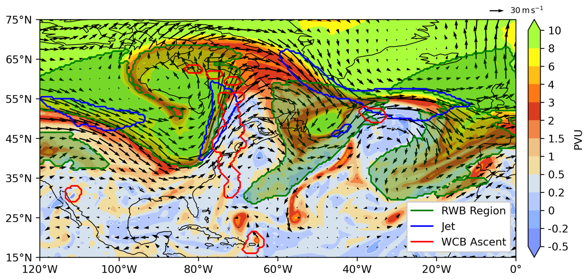
Figure 1 Weather feature masks overlaid on an isentropic PV map (colour, PVU) at 340 K at 00:00 UTC on 29 August 2019. The green contour with shading indicates the RWB region (see text for details), the blue contour the upper-level jet stream, and the red contour the WCB ascent. Arrows show wind speed and direction on the same isentrope.

2.2 In situ commercial aircraft EDR measurements

The aircraft data used in this study is obtained from the International Air Transport Association (IATA) Turbulence Aware historical data archive (IATA, 2022), covering the period from January 2019 to September 2022. Apart from traditional meteorological variables reported by aircraft, each report also includes the 1 min mean and peak values of EDR (${\mathrm{m}}^{\mathrm{2}/\mathrm{3}}{\mathrm{s}}^{-\mathrm{1}}$), which are estimated using the automated algorithm developed by the National Center for Atmospheric Research (Sharman et al., 2014; Meymaris et al., 2019). The EDR values are estimated from the vertical wind time series every minute and it is routinely reported every 15 to 20 min. Additional reports are triggered if the peak EDR exceeds predefined thresholds and these reports have the original 1 min resolution. The data is anonymous with all information related to aircraft and airlines masked. The major steps taken during quality control and event identification are outlined below and a description of the technical details is given in Appendix A.

After removing data with quality issues, only measurements above 20 000 and below 60 000 ft (above 6.1 km and below 18.3 km) are retained to focus on turbulence in the UTLS. The number of reports categorised according to their peak EDR values is summarised in Table 2.

Table 2 Number of turbulence reports from IATA Turbulence Aware at flight altitude above 20 000 and below 60 000 ft after data quality check. Note that observations with EDR ≥ 0.2 ${\mathrm{m}}^{\mathrm{2}/\mathrm{3}}{\mathrm{s}}^{-\mathrm{1}}$ are considered as having moderate-or-greater (MoG) intensity and they build the basis for event identification in this study.

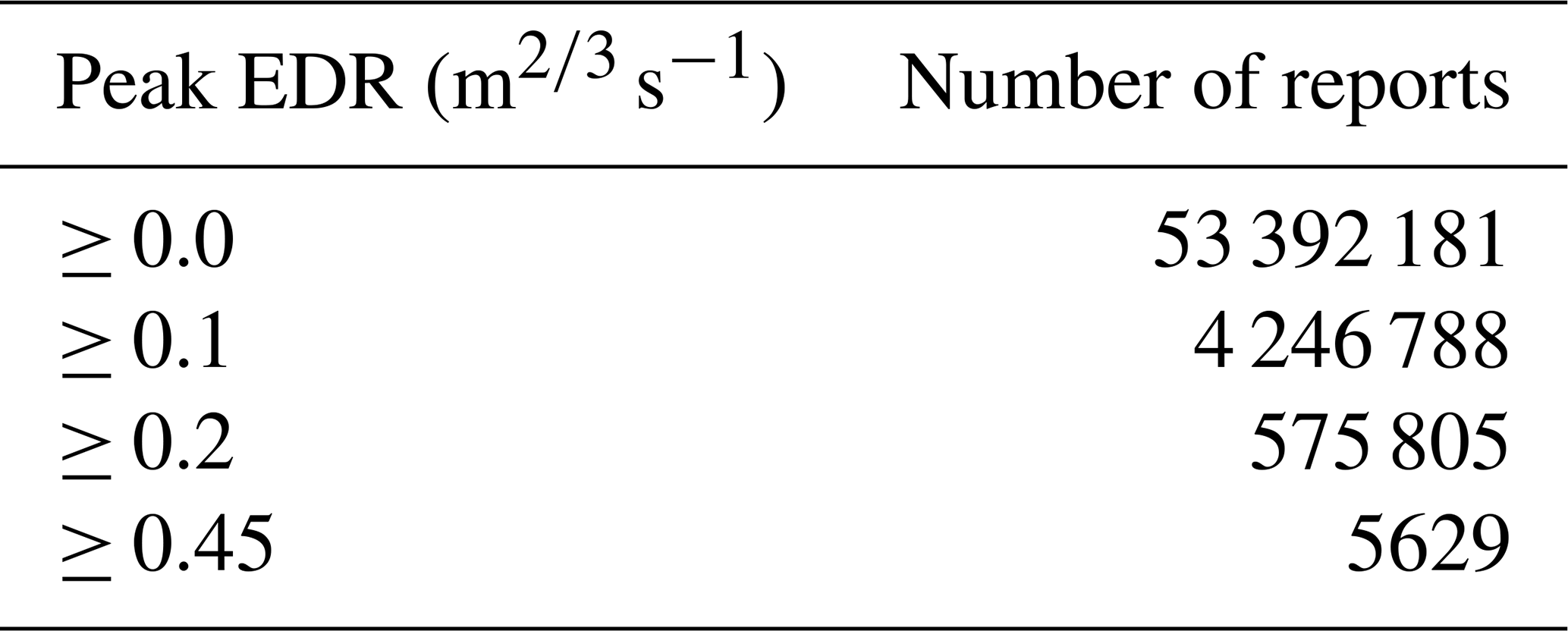
To identify turbulence events, reports with peak EDR values greater than or equal to 0.2 ${\mathrm{m}}^{\mathrm{2}/\mathrm{3}}{\mathrm{s}}^{-\mathrm{1}}$ are first extracted and considered as having moderate-or-greater (MoG) intensity, which follows the definition given by the International Civil Aviation Organization (ICAO) (ICAO, 2018) and this value is similar to previous studies (e.g. Sharman et al., 2014). The MoG reports are then grouped into spatially and temporally coherent events using the Density Based Spatial Clustering of Applications with Noise (DBSCAN) clustering algorithm (Ester et al., 1996) based on their locations and time. The parameters used for the clustering algorithm are set to ensure that each event has a density of at least 10 MoG reports within a time window of 40 min and a circular area of 250 km radius. The geographical distribution of the identified events is shown in Fig. 2. It is clearly seen that the spatial coverage of the data is uneven with sparse events in the Southern Hemisphere but concentrated over the U.S. This sampling bias must be realised when interpreting the results.

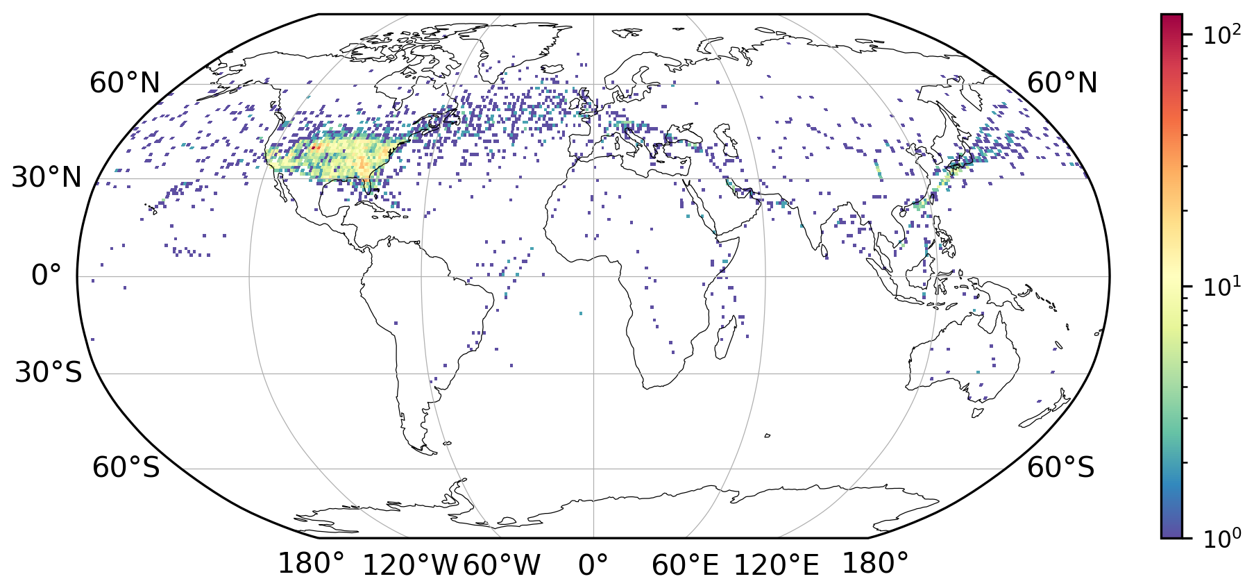
Figure 2 The number of the moderate-or-greater (MoG) turbulence events identified in each 1° × 1° grid box. The number of events is substantially higher over the contiguous U.S. and major flight routes and most of them are in the Northern Hemisphere. Note that the colour scale is logarithmic.

To ensure that the MoG turbulence events identified occur in predominantly clear-air conditions, the globally-merged (60° S–60° N) satellite infra-red brightness temperature data (Janowiak et al., 2017) is employed and used as a proxy for cloud top temperature. Events having more than half of their reports below cloud top (temperature higher than the brightness temperature) are considered as in-cloud events while the remaining events are considered as predominantly clear-air (clear-air or near-cloud) events. A total of 4880 events in the Northern Hemisphere are retained after filtering and they are the primary data used in the event-based analysis. The report with the maximum peak EDR value in each event is used to characterise the entire event in terms of location, time, and intensity.

All reports (including those with peak EDR < 0.2 ${\mathrm{m}}^{\mathrm{2}/\mathrm{3}}{\mathrm{s}}^{-\mathrm{1}}$) are also assigned to their corresponding nearest model grid point (0.5° regular latitude–longitude grid and vertical model levels of ERA5 reanalysis data) and the nearest hourly time step. The altitude is converted into pressure using the International Standard Atmosphere (ISA) (NOAA et al., 1976) during the process. At each grid point, only the maximum peak EDR value of the reports assigned is retained to address the intermittent nature of turbulence. Grid points that have zero assigned reports are filled with missing values. The resultant three-dimensional field of peak EDR is then available for each time step and the data is termed “grid point EDR”. This data is utilised subsequently together with ERA5 reanalysis when obtaining grid point-based statistics. The term “grid point” will be used in subsequent sections to describe the four-dimensional space-time grid points. “Horizontal grid point” will be used if only the horizontal locations are of interest.

2.3 Weather features mask-matching

To examine the linkage between different weather features and the observed turbulence events, a mask-matching method is developed to determine if a turbulence event is associated with a weather feature. It is assumed that the association is reflected in the spatial proximity and a close proximity is required for potential linkage. In addition, a measure for the extent of overlap is used to better associate events that are near but not within the mask of the corresponding weather feature, since only considering the presence of the mask at the event centre will miss these potential linkages.

The weather feature masks are first interpolated to a translated latitude–longitude grid with its origin being the event location and grid points within 1000 km from the event are extracted. The interpolation is needed to minimise the distortion due to the poleward convergence of longitudes and the same technique is used also for the event-centred composites (Sect. 3.1). The 1000 km radius is chosen from the typical spatial scale of synoptic features and this region is considered the neighbourhood of the event. A weighted sum of the number of grid points being covered by the weather system mask is calculated and the weight function is inversely proportional to distance squared r², with value capped at $\frac{\mathrm{1}}{{\mathrm{100}}^{\mathrm{2}}}$ km⁻² for points less than 100 km away from the event. The distributions of the weighted sum (Fig. S6) are examined for different weather features and most of them show a separation between clusters representing minimal (low values) and maximal (high values) overlap. A threshold value of 0.0015 km⁻² is chosen with the aim to remove the cluster that has zero or minimal overlap of the weather feature mask with the event neighbourhood. If the weighted sum has a higher value, the event is considered to be associated with the weather feature, or concurrent with this weather feature. This concurrence definition is used to categorise an event according to its associated weather features.

3 Results

3.1 Event-centred composites

The environmental conditions associated with the 4880 MoG turbulence events are explored using event-centred composites. The environmental fields on the pressure or potential temperature level of each event are extracted from the nearest hourly time step, interpolated to the same latitude-longitude grid centred at the event location (cf. Sect. 2.3), and averaged to construct the composites. Several well-known characteristics of the environmental conditions associated with CAT are revealed in these composite fields (Fig. 3). The events on average are located close to the dynamical tropopause, which is indicated by the proximity between the event location and the 2 PVU isoline in the isentropic PV composite (Fig. 3a). The frequency of finding Ri < 1 sharply peaks at the event location (Fig. 3b), which suggests that many events likely occurred in the presence of KHI. The threshold value of Richardson number is chosen to be 1 as it is consistent with other studies using reanalysis data (e.g. Lee et al., 2023) and the distribution of subcritical Richardson number in reanalysis data is found to be more consistent with that in radiosonde observation using this threshold (Shao et al., 2023). When the upper-level jet stream, as a weather feature mask (see Sect. 2.1), is considered, a region with high occurrence frequency of over 0.4 is found surrounding the event location (Fig. 3c), which corroborates the close linkage between upper-level jet streams and CAT revealed by previous case studies.

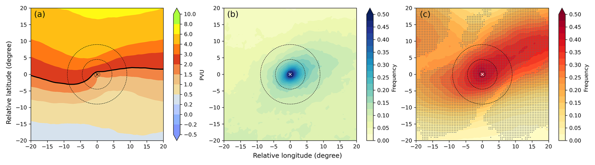
Figure 3 Event-centred composites of (a) isentropic PV, (b) frequency of Ri < 1, and (c) frequency of upper-level jet stream mask. The isentropic and isobaric surfaces at which the events occur are used for (a) and (b) respectively. The event location is denoted by the cross at the centre and the dashed circles indicate 100, 500, and 1000 km distance from it. The black contour in (a) indicates the 2 PVU isoline, which defines the dynamical tropopause. The grid points stitched with grey dots in (c) show locations where the frequency exceeds the 99.5th percentile or falls below the 0.5th percentile of the randomly sampled distribution (see text for details).

Apart from results that confirm the findings of earlier research, the weather feature mask composites hint towards unexplored relationships between CAT and RWB or WCB. The RWB region has a high frequency of occurrence in the neighbourhood of the events, with a maximum of above 0.5 located further northwest and about 0.38 at the event location (Fig. 4a). A distinct peak in occurrence frequency for WCB ascent is positioned right at the event location (Fig. 4b). Though the peak frequency of around 0.25 is comparatively lower, it is still striking as the WCB ascent masks are generally spatially confined. Also, since the WCB ascent mask represents the ascending phase of the trajectories in the mid-troposphere (500 to 800 hPa), it means that around one-fourth of the events coincided with the mask and occurred at locations where air is rapidly ascending. As all reports considered are above 20 000 ft, corresponding to 466 hPa in the ISA, they may be found directly coinciding with the ascending airstreams or above them.

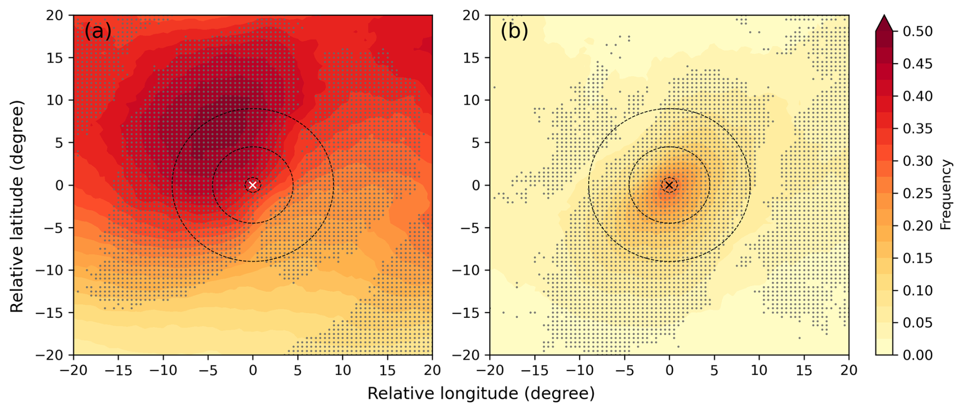
Figure 4 Event-centred composites of (a) frequency of RWB region (projected PV streamer of 305–350 K), and (b) frequency of WCB ascent. The event location is denoted by the cross at the centre and the dashed circles indicate 100, 500, and 1000 km distance from it. The grid points stitched with grey dots show locations where the frequency exceeds the 99.5th percentile or falls below the 0.5th percentile of the randomly sampled distribution (see text for details).

Nevertheless, these peaks in occurrence frequencies of these weather feature masks could arise solely by coincidence, for instance, due to the local characteristics of the event locations. To check if these weather features occur more frequently or less frequently with the turbulence events compared to the climatological conditions, a random-sampling approach is employed. The time of an event is randomised by assigning it another time within the same season and 1000 sets of randomised events are generated, which gives a distribution of the occurrence frequency at each grid point. The actual composite is then compared to the distribution and grid points having values above the 99.5th percentile or below the 0.5th percentile are stitched with grey dots in Figs. 3c and 4. The peaks discussed earlier are all above the 99.5th percentile of the randomised distribution, which suggests that they are unlikely the result of coincidence. In particular, the high occurrence frequencies of RWB regions and WCB ascents with the events indicate that RWB and WCB are potentially related to the occurrence of CAT.

The composites of other weather features (Fig. S1 in the Supplement) are examined but they either show similar patterns as they are physically related (e.g. surface cyclones and WCB ascents) or have a low occurrence frequency (e.g. tropopause folds). The other weather features will therefore not be discussed further. Note that the spatial patterns of the weather feature composites should be interpreted carefully due to the sampling bias mentioned in Sect. 2.2. For instance, it might be tempting to conclude that events occur more frequently near the jet entrance when Fig. 3c is considered. However, since the atmosphere is not evenly sampled, this spatial pattern may also emerge as the jet entrance is better sampled by aircraft. A discussion on the effect of this sampling bias, particularly for the geographical locations, is included in Sect. 4.1.

3.2 Weather feature-based typology

To further examine the linkage between weather features and CAT, the events are categorised according to their concurrent weather features, using the matching method discussed in Sect. 2.3. Motivated by the event-centred composite results, the upper-level jet stream, RWB region, and WCB ascent are the three weather features considered when defining the categories. As the weather features are not independent of each other, events can be concurrent with more than one. When selecting two features A and B for categorisation, the overlapping fraction $\frac{N(A\cap B)}{N(A\cup B)}$ has the lowest value of 15.6 % when RWB region and WCB ascent are chosen, while the upper-level jet stream has a value of 29.7 % and 37.3 % when paired with RWB region and WCB ascent respectively. The RWB region/WCB ascent pair is therefore selected for defining the categories and it also facilitates the analysis of the unexplored relationships between these two weather features and CAT. This choice, while inevitably being subjective to a certain extent, will be shown reasonable when the associated environmental conditions of the categorised events are examined. The upper-level jet stream, however, is important as well and it will be discussed later in Sect. 4.2.

The events are allocated to three mutually exclusive categories. Type I are events concurrent with RWB region but not with WCB ascent while type II are all events concurrent with WCB ascent. The remaining events are collectively referred to as “remainder”. The WCB ascent concurrent events form one category by itself because the WCB ascent mask has a spatial coverage much smaller than that of RWB region. Physically, type I is therefore the group of events concurrent with RWB while type II is the group of events occurring above WCB ascent. The number of events in each category is tabulated in Table 3 and their corresponding geographical distributions are shown in Fig. 5.

Table 3 Number of MoG turbulence events in each weather feature-based category.

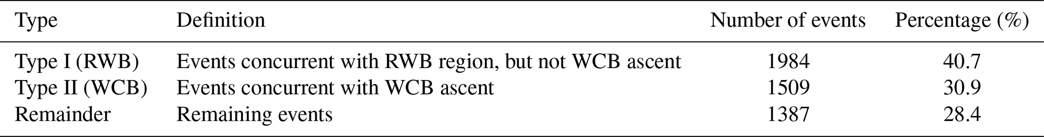
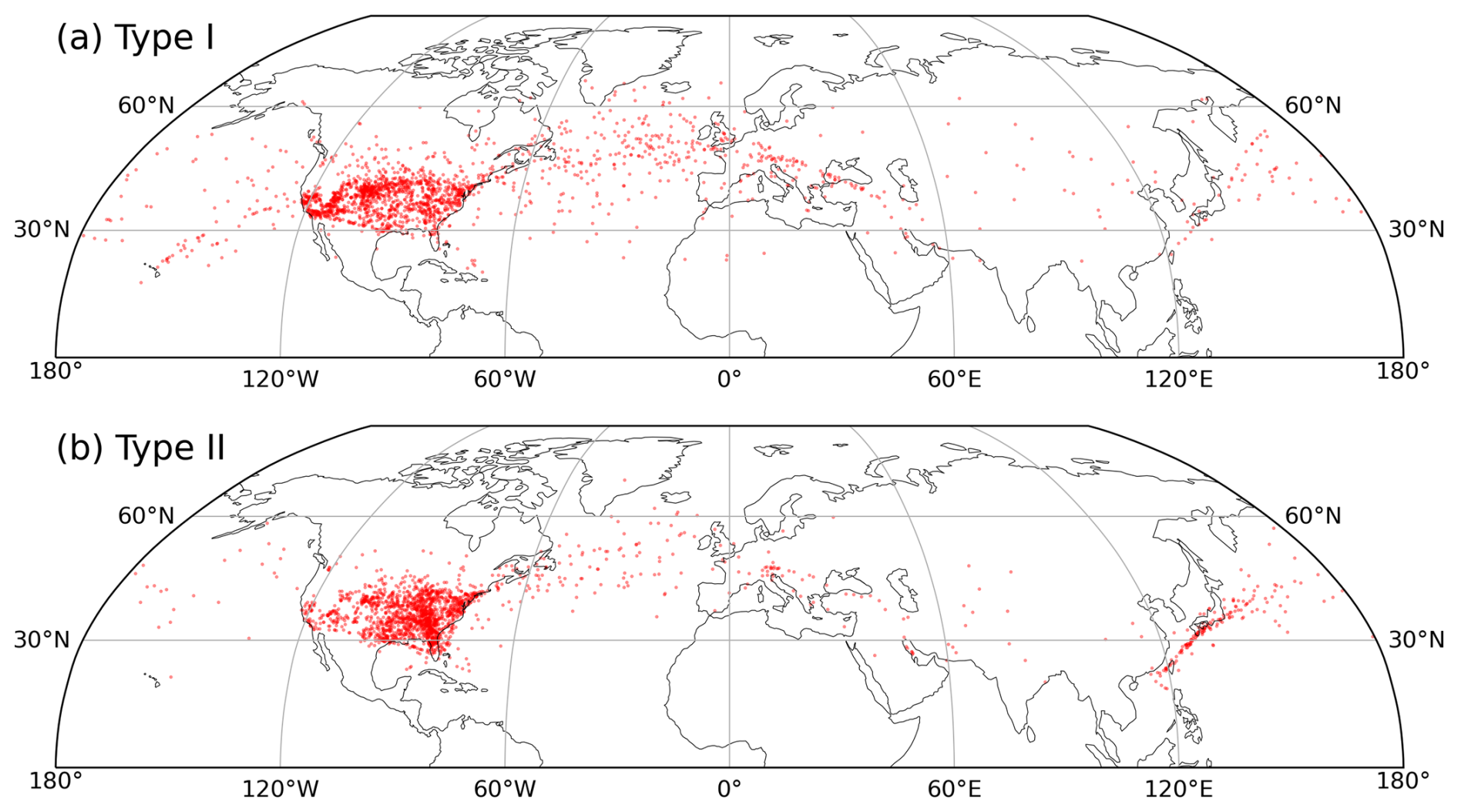
Figure 5 Geographical distribution of (a) type I and (b) type II events. The location of an event is determined by the report with the highest peak EDR value and each event is indicated by a red dot.

The three categories have comparable numbers of events and have an approximately 40 %–30 %–30 % partition (Table 3). When comparing the geographical distribution, type II events are found concentrated over the eastern part of the U.S., while type I events are more evenly distributed over the contiguous U.S. Type II events also have a higher density over the western Pacific, particularly in the East China Sea when compared to type I. The geographical distribution of type II events can be understood as these regions are storm track regions, where peaks of WCB ascent occurrence frequency are found as well (Fig. S3). The type I distribution also matches the climatological distribution of RWB regions (Fig. S2), where there is a continuous band of high occurrence frequency over the west coast of the U.S. Note that since the two weather features are mainly found in the extratropics, these two types of events also lie in this latitude band. The events found in the tropics are mostly classified into the remainder (Fig. S4).

The differences in the environmental conditions associated with these two types of events are analysed by comparing the composite fields for each category. First, type I events stand out with substantially higher values (around 50 % higher) of horizontal deformation in the immediate neighbourhood of the events when compared to the other two categories (Fig. 6) with the peak of horizontal deformation pinpointing the event location. RWB is known to be associated with high horizontal deformation (Spensberger and Spengler, 2014) and high horizontal deformation is also a well-known physical quantity useful for CAT forecasting (e.g. Endlich, 1964; Ellrod and Knapp, 1992). We may hence postulate a linkage between RWB and CAT, bridged by high horizontal deformation.

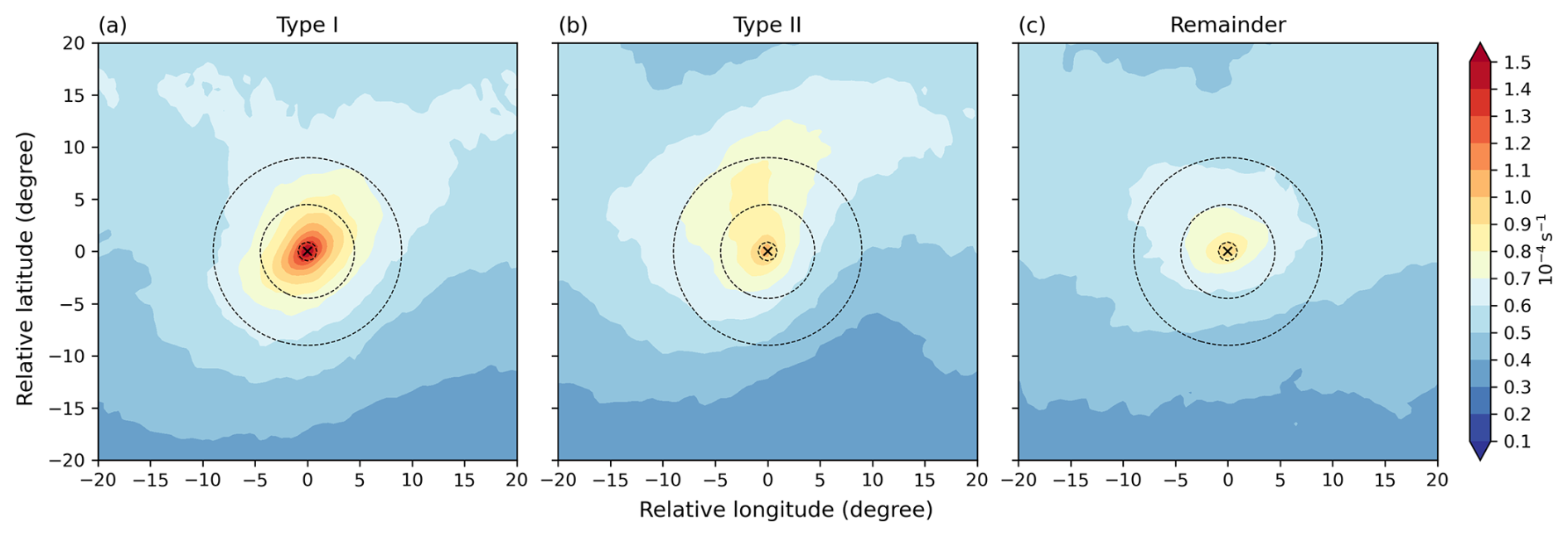
Figure 6 Composites of horizontal deformation (colours) on the isobaric surface of the MoG turbulence events for (a) type I, (b) type II, and (c) remainder events. The event location is denoted by the cross at the centre and the dashed circles indicate 100, 500, and 1000 km distance from it.

Second, type II events differ from the other two categories by having a peak in the occurrence frequency of negative PV (Fig. 7) and a much higher cloud ice water content (Fig. 8) near the event location. Though there is also a high occurrence frequency of negative PV near the events for the remainder category, the peak in the type II composite is enhanced notably from background values, which increase equatorward (e.g. see Thompson et al., 2018), making type II different from the remainder. The significantly higher cloud ice water content also indicates that some of the type II events are more likely to be near-cloud turbulence (Lane et al., 2012), as in-cloud events are removed (see Sect. 2.2). These two observations are consistent with the fact that convection and cloud formation are common in WCB ascent and the associated latent heating maximum in clouds reduces PV above it (Madonna et al., 2014; Heitmann et al., 2024). Negative PV is relevant for CAT occurrence as it indicates the presence of instability. A further examination of the events with negative PV at the event location reveals that static instability (N² < 0) can only account for less than 3 % of these negative PV values. Hence, most negative PV values would be the result of the presence of inertial or symmetric instability. Since inertial or symmetric instability has been suggested to be a possible cause of CAT in previous studies (e.g. Knox, 1997), WCB ascent may potentially favour the occurrence of CAT by creating an environment conducive to this instability.

Figure 7 As Fig. 6, but for the frequency of negative PV.

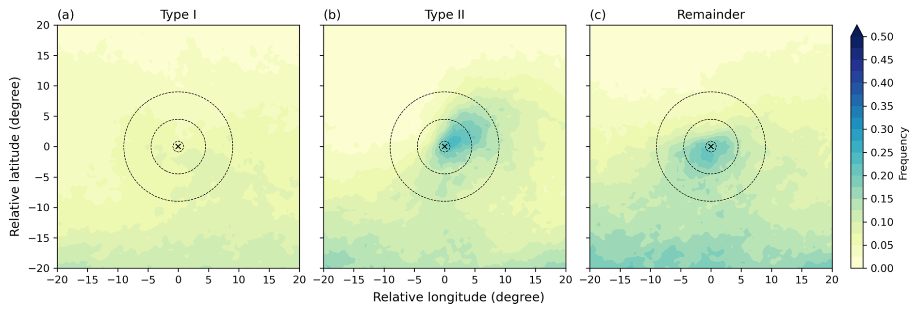
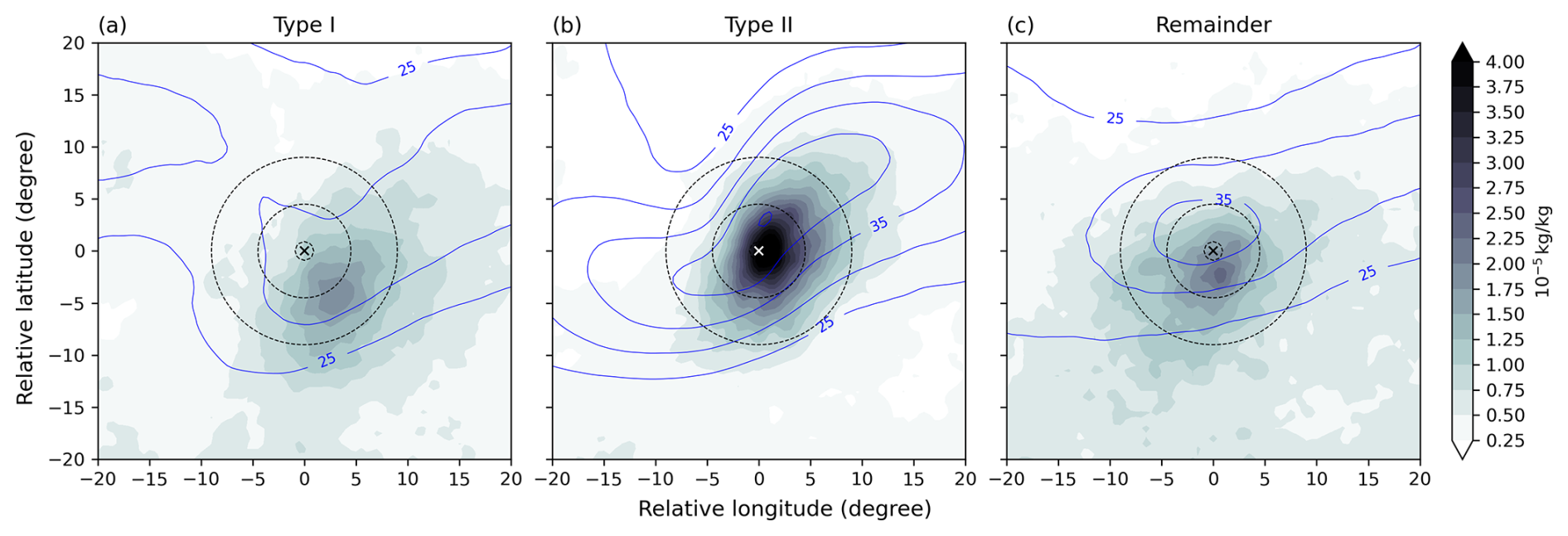
Figure 8 As Fig. 6, but for cloud ice water content (colours) and wind speed (blue contours). The wind speed contours start from 25 m s⁻¹ with a contour interval of 5 m s⁻¹.

On the other hand, when the wind speed composite is examined, it is revealed that type II events are associated with much stronger winds, aligning in a southwest-northeast direction (Fig. 8). This result is similar to the analysis of a case study by Trier et al. (2020), who showed that the convective outflow from an extratropical cyclone (which is likely the outflow from a WCB) strengthens the upper-level wind. They further suggested that the vertical shear layers above and below this outflow are responsible for the numerous turbulence reports by aircraft for their case, as local KHI or static instability is triggered. The strengthening of the upper-level wind, and hence shear may also be linked to the higher occurrence frequency of negative PV concurrent with WCB ascent. Harvey et al. (2020) suggested that negative PV can be formed by the diabatic heating associated with WCB in the presence of vertical wind shear. Oertel et al. (2020) showed that the upper-level negative PV induced by embedded convection in WCB can aggregate to a coherent structure and strengthen the isentropic PV gradient near the upper-level jet, which in effect accelerates the local flow (Lojko et al., 2025). The northward extension of the horizontal deformation pattern in Fig. 6b for type II events may also be linked to this accelerated flow if the negative PV is situated on the equatorward flank of the jet stream. Therefore, the negative PV associated with WCB ascent may also indirectly lead to the occurrence of CAT by the enhancement of wind speed and shear at upper levels.

Third, while both type I and II events show similar frequencies of having Ri < 1 in their proximity, there are differences in the underlying vertical wind shear and stratification. Despite the slightly different shapes, a peak in the occurrence frequency of Ri < 1 is always found at the event location for all three types (Fig. 9). This implies that KHI is not tied to a particular synoptic type and it is likely an important mechanism in causing CAT for all three types of events. Nevertheless, the vertical wind shear and stratification composites of type I and II are contrasting (Fig. 10). In type I events, vertical wind shear is enhanced sharply in the confined neighbourhood of the events, where the static stability due to stratification is usually increased locally. Conversely, the enhancement of vertical wind shear for type II events is less prominent at the event location and spreads spatially across a larger area where wind speed is high (Fig. 8), while the static stability at the event location and its downstream region is reduced. Therefore, although type I events are on average situated in a more sheared environment than type II events, the environment is correspondingly more stable statically for type I events compared to type II events, which may explain the similar occurrence frequencies of potential KHI as shown in Fig. 9.

Figure 9 As Fig. 6, but for the frequency of Ri < 1.

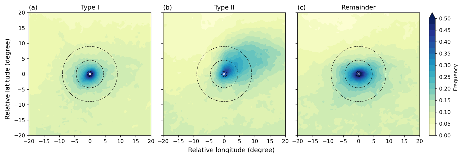
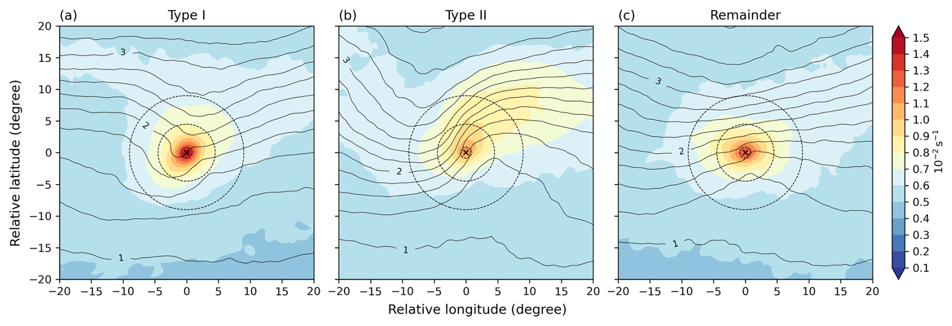
Figure 10 As Fig. 6, but for vertical wind shear (colours) and the square of Brunt–Väisälä frequency (N² = $\frac{g}{\mathit{\theta }}\frac{\partial \mathit{\theta }}{\partial z}$, black contours). The contours of N² start from 1 × 10⁻⁴ s⁻² with a contour interval of 2.5 × 10⁻⁵ s⁻². The contour labels have the unit of 10⁻⁴ s⁻².

Finally, the differences in environmental conditions also affect the performance of the (Ellrod) Turbulence index (TI) (Ellrod and Knapp, 1992) to capture the observed CAT events. As already discussed, both the horizontal deformation and vertical wind shear are lower in type II events compared to type I on average. Since TI1 is the product of horizontal deformation and vertical wind shear (Table 1), its value at the event location in the composite field is much lower for type II (not shown). When TI2 is considered (Fig. 11), which subtracts horizontal divergence from horizontal deformation before multiplying this difference by the vertical wind shear (Table 1), an even larger difference is observed as type II events are usually accompanied by a horizontally divergent outflow (Fig. 11), as WCB ascent transport air vertically upward into the tropopause region. As the TIs are designed to capture turbulence related to frontogenetic processes (Ellrod and Knapp, 1992), the lower values of TIs are reasonable and imply that type II events are more likely to be caused by other processes, which may be moist processes during WCB ascent as mentioned (Madonna et al., 2014). It also demonstrates again that multiple turbulence diagnostics are required in capturing different types of CAT (Sharman et al., 2006). For instance, high TIs are better at capturing type I events, but diagnosing negative PV may be required to identify type II events. The origin of these differences also traces back to the underlying synoptic and mesoscale weather features that shape the environmental conditions.

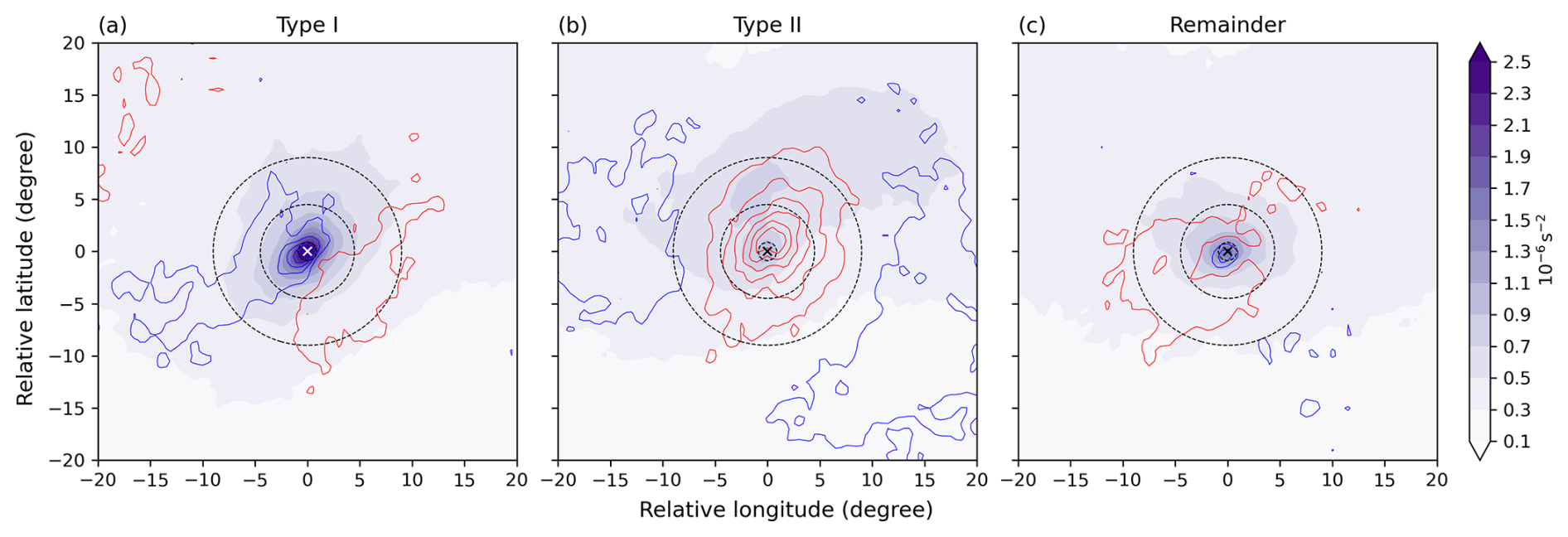
Figure 11 As Fig. 6, but for Turbulence index 2 (colours) and horizontal divergence (contours). Red and blue contours indicate horizontal divergence and convergence, respectively, starting from ±2 × 10⁻⁶ s⁻¹ and increasing/decreasing with a contour interval of 4 × 10⁻⁶ s⁻¹.

Summarising the results, the categorised composites reveal different characteristics of the environmental conditions for the type I and II events. Type I events, which are linked with RWB, have substantially higher horizontal deformation. RWB is potentially conducive to the occurrence of CAT by generating high horizontal deformation in the environment. In contrast, type II events, which are linked with WCB ascent, are more likely near-cloud events. A higher occurrence frequency of negative PV and strengthened wind speed are found near type II events. The two observations are understandable when the moist processes and the outflow associated with embedded deep convection in WCB are considered. Though both types of events have similar concurrence frequency with potential KHI, those for type II are found in less sheared, but less statically stable layers compared to type I. These differences in the environments of the two types of events may also determine the effectiveness of certain turbulence diagnostics in capturing that type of CAT.

3.3 Coincidental or correlated?

At this point, the results obtained from the categorised composites can be questioned: What if the physical quantity concerned, for instance, horizontal deformation for type I events, is only tied with the weather feature but not the occurrence of turbulence? i.e. the same or similar composite will be obtained if we randomly pick locations that satisfy the mask-matching criteria, regardless of whether the location is turbulent or not. The justification given in the previous section relies on the results from other studies, but it can also be answered with the grid point EDR data (see Sect. 2.2). The analysis of this grid point-based statistics can also assess the importance of a weather feature in providing the corresponding environmental conditions conducive to the occurrence of CAT.

The relationships between RWB, horizontal deformation, and CAT, which concern type I events according to the categorisation scheme, are first discussed. As mentioned in Sect. 2.2, all reports, including reports that are below moderate turbulence intensity (peak EDR < 0.2 ${\mathrm{m}}^{\mathrm{2}/\mathrm{3}}{\mathrm{s}}^{-\mathrm{1}}$) are utilised to generate the grid point EDR data. All grid points that have assigned in situ EDR measurements are selected and the corresponding values of horizontal deformation and the weather feature masks are extracted from ERA5 reanalysis (since weather feature masks are two-dimensional, the same value is obtained for grid points from the same vertical column). Only grid points that are considered to be in clear-air, which means the temperature of the grid point is lower than the satellite infra-red brightness temperature (details are given in Appendix A3), are selected. The grid points are then sorted in ascending order according to their horizontal deformation values and divided into 100 bins using the percentile values, such that each bin has the same number of grid points (1 % of the total). The first bin then covers horizontal deformation values below the 1st percentile, the second bin covers values between the 1st and the 2nd percentile, and so on. The values of the bin centres are indicated by the blue curve in Fig. 12a.

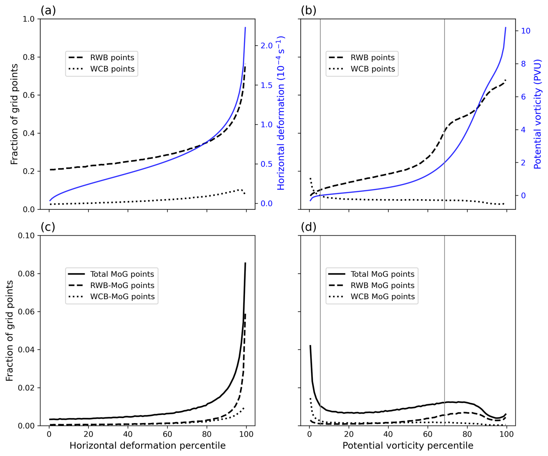
Figure 12 Fraction of grid points that fulfil a certain condition as a function of (a, c) horizontal deformation and (b, d) PV (values in the Southern Hemisphere have their sign reversed). The fraction is calculated within each of the 100 equally sized bins, which are defined by the corresponding percentiles. The number of grid points covered by the RWB region mask but not the WCB ascent mask (dashed line, labelled as “RWB”), and the number of grid points covered by the WCB ascent mask (dotted line, labelled as “WCB”) are divided by their corresponding bin total and plotted in (a) and (b). The values of the bin centres are also plotted in blue (a, b), with the scales indicated by the vertical axis on the right. Similarly, the fractions of the total number of MoG points, RWB MoG points, and WCB MoG points are indicated by the solid, dashed, and dotted lines respectively in (c, d). Note the different scales used in the y axis for the two rows. The vertical lines in (b, d) are plotted to indicate the bins that cover PV values of 0 and 2 respectively. See text for details.

The number of grid points that are covered by weather feature masks, using the categorisation types, are then counted in each bin and plotted as a fraction normalised by the number of grid points in each bin (Fig. 12a). The dashed and dotted black lines indicate type I (covered by the RWB region but not WCB ascent mask, labelled as RWB points) and type II (covered by WCB ascent mask, labelled as WCB points) respectively. If the weather feature is not correlated with horizontal deformation, the distribution should be random and an even distribution is expected. However, the fraction of RWB points in a bin increases when going from low to high horizontal deformation bins and it increases particularly rapidly above the 85th percentile (Fig. 12a), reaching values over 0.5. This suggests that RWB points have a skewed distribution of horizontal deformation towards higher values and a large portion of grid points with high horizontal deformation are connected to RWB conditions.

The fraction of grid points with EDR ≥ 0.2 ${\mathrm{m}}^{\mathrm{2}/\mathrm{3}}{\mathrm{s}}^{-\mathrm{1}}$, named “MoG points”, are also counted in each bin and this is shown by the solid line in Fig. 12c. The fraction of MoG points grows drastically from around 0.01 to 0.08 when moving towards high horizontal deformation bins, which indicates that the chance of encountering MoG turbulence is enhanced in a high horizontal deformation environment. Similar to Fig. 12a, the fractions of MoG points which are covered by weather feature masks are also counted and plotted in Fig. 12c. When comparing the two types considered, the majority of MoG points in high horizontal deformation belong to RWB points, which shows that RWB is frequently found at MoG points with high horizontal deformation and is dominating. With the numbers of RWB points, MoG points, and RWB-MoG points (grid points being both RWB and MoG points) all increasing sharply at the high horizontal deformation bins, it is plausible that the high horizontal deformation associated with RWB is conducive to the occurrence of CAT.

The same analysis is performed for PV, which focuses on the relationships between negative PV, WCB ascent, and CAT, and the results are shown in Fig. 12b, d. First, when examining the distribution of PV as shown with the blue curve in Fig. 12b, the two bins which contain PV values of 0 and 2 respectively are selected and indicated by the left and right vertical grey lines in the figure. The bins are then separated into three groups, with the leftmost bins (5 % of the grid points) having negative PV values, the middle bins (64 % of the grid points) having ordinary tropospheric PV values, and the rightmost bins (31 % of the grid points) having PV values greater than 2 PVU and considered mainly stratospheric.

When focusing on the bins with negative PV (the leftmost region of Fig. 12b), the fraction of grid points belonging to the WCB category increases notably compared to the other bins and it reaches values up to around 0.16. This sharp increase indicates that WCB ascent has a higher occurrence frequency in an environment with negative PV, though quite a large portion of negative PV grid points is still found in regions without WCB ascent. Therefore, WCB ascent is likely only one of the weather systems or features that generate negative PV. In Fig. 12d, the fraction of MoG points increases substantially in the negative PV bins, which is consistent with the suggestion that MoG turbulence is more frequently encountered in the presence of inertial or symmetric instabilities, or the indirectly enhanced shear. Also, a significant increase in WCB-MoG points can be found in the negative PV bins and it accounts for around 20 % to 35 % of the MoG points in these bins. Collectively, the data indicate that a linkage between the negative PV associated with WCB ascents and the occurrence of CAT exists, but many MoG points with negative PV are potentially linked with other weather systems or features as well, for instance, organised convection or squall lines (Trier and Sharman, 2016). It is also interesting to note that the fraction of MoG points starts to decrease when PV values get above 2 PVU, as the stratosphere in general has higher static stability and suppresses turbulence (as can be observed in the corresponding analysis using stratification, not shown). The slight increase in the number of MoG points in the highest PV bins might be explained by the occurrence of CAT in high horizontal deformation environments as horizontal shear is also a component of vorticity. This possibility is consistent with the result discussed previously concerning the RWB points as the number of RWB-MoG points also increases in these bins.

The results from the grid point-based analyses agree with those from categorised composites in Sect. 3.2 and complement them with an assessment on how important the corresponding weather feature is in generating the CAT-conducive environment. To assess if there is geographical dependence of the importance of the respective weather features in MoG turbulence encounters, the MoG points with horizontal deformation above the 95th percentile or negative PV are selected for further examination at each horizontal grid point. In Fig. 13a, the percentages of MoG points with high horizontal deformation at each horizontal grid point being RWB MoG points are plotted. Percentages of over 60 % are found in the western U.S., showing that RWB accounts for a large majority of CAT encounters with high horizontal deformation in this region. The percentages are lower over the eastern U.S., but RWB is still responsible for around 30 to 50 %. For the negative PV MoG points (Fig. 13b), WCB ascent accounts for around half of the points in the eastern U.S. However, the contribution to negative PV from WCB ascent decreases considerably in the tropics compared to the extratropics, as the more prominent localised convective activities may also generate negative PV. This possibly also explains the low fraction of WCB points in negative PV bins shown in Fig. 12b.

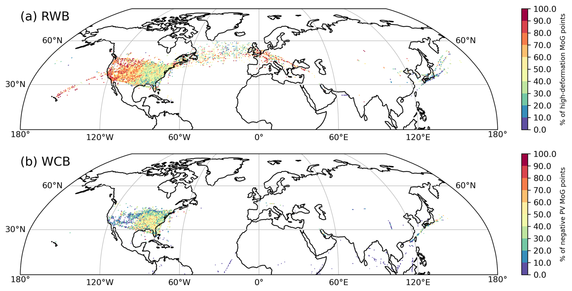
Figure 13 The percentages of (a) MoG points with top 5 % horizontal deformation covered by RWB region mask but not WCB ascent mask and (b) MoG points with negative PV covered by WCB ascent mask. The values are determined at each 0.5° × 0.5° horizontal grid point and only horizontal grid points with at least 5 available data points are shown.

To conclude, the grid point-based statistics plausibly indicates that the high horizontal deformation concurrent with RWB and negative PV associated with WCB ascent are correlated with the enhanced chance of CAT encounter, which supports the relationships already hinted at by the categorised composites. Moreover, the relevance or importance of RWB and WCB ascent in generating the two CAT-conducive environments also varies geographically, with RWB being the dominant driver of MoG turbulence with high horizontal deformation over the western U.S. and WCB ascent (possibly with embedded convection) contributing significantly to the MoG turbulence with negative PV in the eastern U.S.

4 Discussion

4.1 Regional dependence

While the composite fields in Sect. 3 are useful in depicting the averaged environmental conditions associated with the turbulence events, variability exists among events as demonstrated when considering events in different geographical regions. As an example, the event-centred composite frequencies of the upper-level jet stream mask are shown for different longitude bands in Fig. 14. Regional differences are clearly discernible, which include both variations in the magnitude and the spatial pattern of the occurrence frequency. First, the frequency of having the upper-level jet stream in the neighbourhood of the turbulence events over the Eurasian continent is less than 0.25 (Fig. 14c), which is much lower than in the other four regions, where at least a frequency of 0.38 is reached. Furthermore, the spatial patterns are significantly different in the other four regions, with the events often located near the jet entrance in the western and eastern U.S. (Fig. 14d, e), while they are found frequently in the vicinity of the jet exit over the North Atlantic (Fig. 14a). The North Pacific basin shows a relatively continuous band of high jet frequency (Fig. 14c), which may results from a superposition of these two patterns.

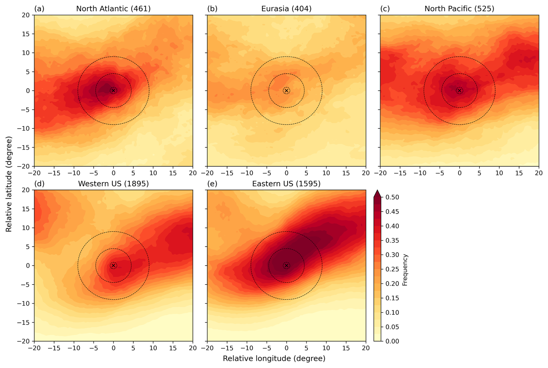
Figure 14 Event-centred composite frequency of the upper-level jet stream mask in (a) North Atlantic (60° W–0°), (b) Eurasia (0°–120° E), (c) North Pacific (120° E–120 ° W), (d) western U.S. (120–90° W), and (e) eastern U.S. (90–60° W). The number of events in each region is indicated in brackets.

This regional decomposition revealed that the spatial pattern that stands out in Fig. 3c is mainly a combination of the prominent patterns found in the western and eastern U.S., since the U.S. airspace is better sampled by the denser air traffic and higher number of aircraft that participate in the IATA Turbulence Aware programme (Fig. 2). This sampling bias is inherent to all studies based on observations and it has to be accounted for when interpreting the composite results. For instance, one may conclude that CAT is more frequent at the jet entrance compared to other parts of the jet given the northeastward extension of the frequency maximum shown in Fig. 3c. However, turbulence near the jet exit may also be frequent over the North Atlantic, but it is undersampled. Other evidence or more observations will be needed to verify such a conclusion. The sampling bias has a greater effect on the event-centred composites (Sect. 3.1) compared to the composites of the categorised events (Sect. 3.2), as events of the same type share the presence of the same weather feature in their neighbourhood, which likely creates similar environmental conditions despite different geographical locations.

4.2 On the role of upper-level jet streams for CAT

Apart from illustrating the regional variability, Fig. 14 also explains the complexity of analysing events concurrent with the upper-level jet stream and the reason to exclude it in the categorisation scheme described in Sect. 3.2. While the upper-level jet stream has long been identified as a relevant weather feature for the occurrence of CAT (Bannon, 1952), previous studies have shown that the mere presence of high wind speed is not necessarily a good predictor of CAT (Endlich and McLean, 1965). Case studies showed that different parts or configurations of the jet stream may favour the occurrence of CAT with different underlying dynamics. For instance, while CAT is found in regions of curved jet streams with strong horizontal shear (Endlich, 1964), the dynamics of cyclonically and anticyclonically curved jets are significantly different. The vertical wind shear in anticyclonic flow is enhanced compared to cyclonic flow due to ageostrophic dynamics (Knox, 1997). In addition, the vertical position of the CAT events relative to the jet can be important as the stratification is expected to be stronger in vertically sheared regions within the lower stratosphere than those in the upper troposphere. As shown in Fig. 14, the CAT events appear to occur in different preferential locations relative to the jet stream and they are likely to be caused by different underlying mechanisms. Therefore, future studies which cluster CAT events according to the different characteristics of the associated jet streams may better address this complexity and give insightful results.

4.3 Triggering of CAT by processes at smaller scales

While high horizontal deformation and negative PV are proposed as the potential causes of the two types of CAT events, processes operating at smaller scales that are not resolved by the ERA5 reanalysis are likely involved in the triggering of these events. Although a detailed analysis of these small-scale processes is out of the scope of this study, a brief discussion is included here to address such complexity of CAT generation. For instance, different interpretations exist for the role of horizontal deformation on CAT occurrence. Though high horizontal deformation has usually been linked to upper-level frontogenesis, which may increase vertical wind shear and ultimately lead to KHI and CAT (e.g. Ellrod and Knapp, 1992), it may also be an indication of the generation of gravity waves due to flow imbalance (Knox et al., 2008). In particular, if gravity waves are involved, they may propagate and perturb the environmental conditions further away from the sources, acting as non-local causes of CAT when the perturbed regions become unstable (e.g. creating KHI).

Negative PV can be connected to CAT occurrence non-locally as well through the presence of inertial instability. Gravity waves may be excited during the release of inertial instability (Knox, 1997), which serves as a possible cause of CAT. In a recent idealised simulation of a zonal jet, the circulations associated with the release of inertial instability are found to create sporadic regions of CAT (indicated by high TI2, Thompson and Schultz, 2021), adding another possibility of the linkage between negative PV and CAT at small scales. Furthermore, since type II events are also more likely to be near-cloud events (Lane et al., 2012), moist processes that occur in the neighbourhood may also contribute to the occurrence of these events. Negative PV may thus be considered as an indication of the presence of moist processes. Trier and Sharman (2016) showed in their simulations that mesoscale negative PV is formed in turbulent regions where static stability is reduced due to deep convection. Also, reports of turbulence and regions of local KHI are found in the vertically sheared layers above and below the jet that is strengthened by the convective outflow of an extratropical cyclone (Trier et al., 2020). Consequently, one should acknowledge the multitude and underlying complexity of CAT trigger mechanisms embedded in the major conclusions of this study.

4.4 Implication for CAT avoidance

Though the linkages between the synoptic situations and the two types of CAT events are interesting and novel, one may be curious about their practical relevance to CAT avoidance. While a direct application of the results of this study to current automated CAT forecasting strategies is challenging, we consider the results to be useful in providing further understanding to the users of CAT forecasting products, including the aviation forecasters, airline dispatchers, and pilots. Current CAT forecasting products are based on multiple turbulence diagnostics (e.g. Sharman et al., 2006) or parametrised turbulent kinetic energy (e.g. Goecke and Machulskaya, 2021), which to some extent obscure the physical understanding of the CAT forecasts due to the sophisticated weighting or parametrisation scheme. With the results presented, which provide the characteristic environmental conditions and possible generation mechanisms of CAT under these synoptic situations, forecaster may better interpret and understand the signals from automated CAT forecasts. Furthermore, a continuation of this line of research may update the schematics that summarise the typical synoptic patterns associated with CAT occurrence (e.g. Fig. 1 in Ellrod et al., 2015) with modern data and tools. These simple yet informative schematics may be used for easy communication to dispatchers or pilots, facilitating the exchange between researchers and users in the aviation sector.

Another potential contribution relates to the higher predictability of synoptic patterns, compared to that of CAT in current forecasting systems. While CAT forecasting remains in the short-range, synoptic-scale dynamics are better predicted with a lead time of several days. If these relationships can be incorporated into CAT forecasting strategy, a longer lead time may allow airlines to respond earlier even in route planning stage. Nevertheless, much more research effort is needed before these potential benefits can be realised.

4.5 Weather features and the mean state

The study also provides an alternative perspective to interpret the climatologies of CAT obtained from turbulence diagnostics based on reanalysis (e.g. Jaeger and Sprenger, 2007; Lee et al., 2023). While the regions with high frequencies of CAT identified by the diagnostics are usually interpreted with long-term averaged flow conditions, such as the climatological jets, individual events are likely to occur in environmental conditions that are substantially different from the climatological mean. This study's focus on different weather features, which are the building blocks of the long-term mean flow, may help explore the possible connections between climatologies and individual events. For example, the maxima of the frequency of high horizontal deformation shown by Lee et al. (2023) also coincide with the regions with high RWB frequency (Fig. S2). From the results discussed in Sect. 3.3, the extreme values of horizontal deformation are potentially concurrent with RWB and it may provide a better explanation for the existence of the frequency maxima of high horizontal deformation in areas far from the climatological jet. Similarly, the projected changes of CAT in the future climate are also linked to the changes of the mean state, for instance, an enhanced vertical wind shear associated with a strengthened meridional temperature gradient (Foudad et al., 2024). Though this linkage is plausible and can be supported by data, the current study suggests that future changes of weather features (e.g. Lee, 2022; Joos et al., 2023) in frequency or geographical location may also contribute to future changes of CAT. With CAT being projected to increase by climate models (e.g. Williams and Joshi, 2013; Williams, 2017; Smith et al., 2023; Foudad et al., 2024), understanding the relationships between weather features and CAT is of practical relevance.

5 Conclusions

Based on a multiyear archive of in situ EDR measurements by commercial aircraft, the relationships between CAT and different synoptic weather features are revisited, making use of state-of-the-art reanalysis data. A total of 4880 moderate-or-greater (MoG) turbulence events are identified in predominantly clear-air conditions in the Northern Hemisphere and results consistent with existing understanding of CAT are found using event-centred composites. The high frequencies of RWB and WCB ascent masks of around 0.38 and 0.25 near the event location, respectively, point towards strong linkages of RWB and WCB with CAT.

Inspired by this result, the observed events are categorised based on their concurrence with the RWB and WCB ascent masks. The 40 % of the turbulence events with RWB but no WCB ascent in their surroundings are referred to as type I, while the 30 % of events having WCB ascent in their vicinity are referred to as type II. Concerning the geographical distribution, type I events are comparatively more frequent in the western U.S. and type II events are more frequent in the eastern U.S. and over the East China Sea.

Different characteristics of the environmental conditions for the two types of events are revealed by the categorised composites. The horizontal deformation at event locations is notably higher for type I events and it suggests that RWB may potentially be conducive to CAT occurrence by creating high horizontal deformation. A higher frequency of occurrence of negative PV and higher cloud ice water content surrounding type II events suggests that moist processes associated with the WCB may favour the occurrence of CAT by generating negative PV, enabling inertial or symmetric instabilities. Higher wind speed is also present for type II events, which was argued in other studies to be a cause of CAT as vertical shear is enhanced. As type II events are associated with higher cloud ice water content, they are more likely to be near-cloud events, though all the events were checked to be predominantly in clear-air conditions. The frequencies of having Ri < 1, which indicates the likelihood of KHI, are similar for the two types, but type I events are found in a more vertically sheared environment and type II events are found in a less stratified environment on average. The identification and characterisation of these two types of events, which in total account for around 70 % of the observed events, is a major novelty in this study.

To examine whether the linkages suggested by the composite results between the two weather features and CAT are plausible, all EDR measurements are processed and compared with the relevant physical quantities at the grid point level. By inspecting the distribution of MoG points in clear air, the high horizontal deformation in RWB conditions and negative PV in WCB ascent regions are shown to correlate with enhanced probability of CAT and support the suggested relationships. RWB also accounts for over 60 % of the MoG points with high horizontal deformation occurring in the western U.S., and more than 30 % in the eastern U.S. WCB ascent on the other hand accounts for around 50 % of the MoG points associated with negative PV in the eastern U.S. Combining with the composite field results, the following linkages are suggested:

• RWB can generate high horizontal deformation, which in turn provides an environment favourable for CAT occurrence.

• Diabatic processes associated with WCBs with embedded convection can create negative PV at upper levels, which is conducive to inertial or symmetric instability and may contribute to the occurrence of CAT. A strengthening of the upper-level flow and thus vertical wind shear is another possible cause of CAT concurrent with WCBs.

While processes at smaller scales, including gravity wave emission and moist processes, are not discussed in detail in this study, they are most likely involved in the generation of the turbulent eddies encountered by aircraft.

The two types of events identified also show some resemblance with the flow patterns used for CAT forecasting in the 1970s (Hopkins, 1977). CAT was documented to be more likely to occur during the formation of an upper-level low or at the shear line at the “throat” of the cut-off low (Hopkins, 1977, their Figs. 11 and 12) and the flow patterns are similar to the situations during RWB. CAT was also found to be more likely to occur when there is surface cyclogenesis (Hopkins, 1977, their Fig. 9), which potentially describes the condition associated with some type II cases. A revisit to the topic with modern data may hence provide a better understanding of the underlying physical mechanism responsible for the CAT observed. Also, the study demonstrates the value of in situ observations, and a dataset with denser spatial coverage would improve the robustness of the results. The perspective of weather features or weather systems also bridges the gap between turbulence diagnostics and large-scale flow conditions, which may help interpret the forecasts, climatologies or future changes of CAT.

Appendix A: Details of the Methodology

A1 Turbulence report quality control

The raw data (reports above 20 000 and below 60 000 ft) obtained from the Turbulence Aware archive has several quality issues, which have to be handled before event identification. First, some reports are duplicated or sent to the database multiple times. For those that are identical, only one copy is retained. For some reports which have all measurements being the same but with different time stamps, the earliest report is retained as the later ones are likely to be unwanted duplication and a total of 243 470 reports are removed (0.45 % of the total). Second, some reports contain missing values in the measurements and they (494 reports) are removed. Third, some reports are isolated from all other reports in location and time. Since a normal aircraft should have routine reports every 15 to 20 min (Meymaris et al., 2019), reports having no neighbouring reports in this time window are suspicious. The DBSCAN (Ester et al., 1996) algorithm, which will be described in detail in the next section, is utilised to identify these suspicious reports (considered as noise by the algorithm). The parameters employed (N = 2, ϵ = $\sqrt{\mathrm{2}}$, L = 400 km, T = 1800 s) guarantee that reports which have neighbouring reports not further than 500 km apart within 20 min are retained. A total of 123361 reports are considered suspicious and removed, consisting of 0.23 % of the total number. The remaining 99.32 % of the data is retained and used for subsequent analysis, as tabulated in Table 2.

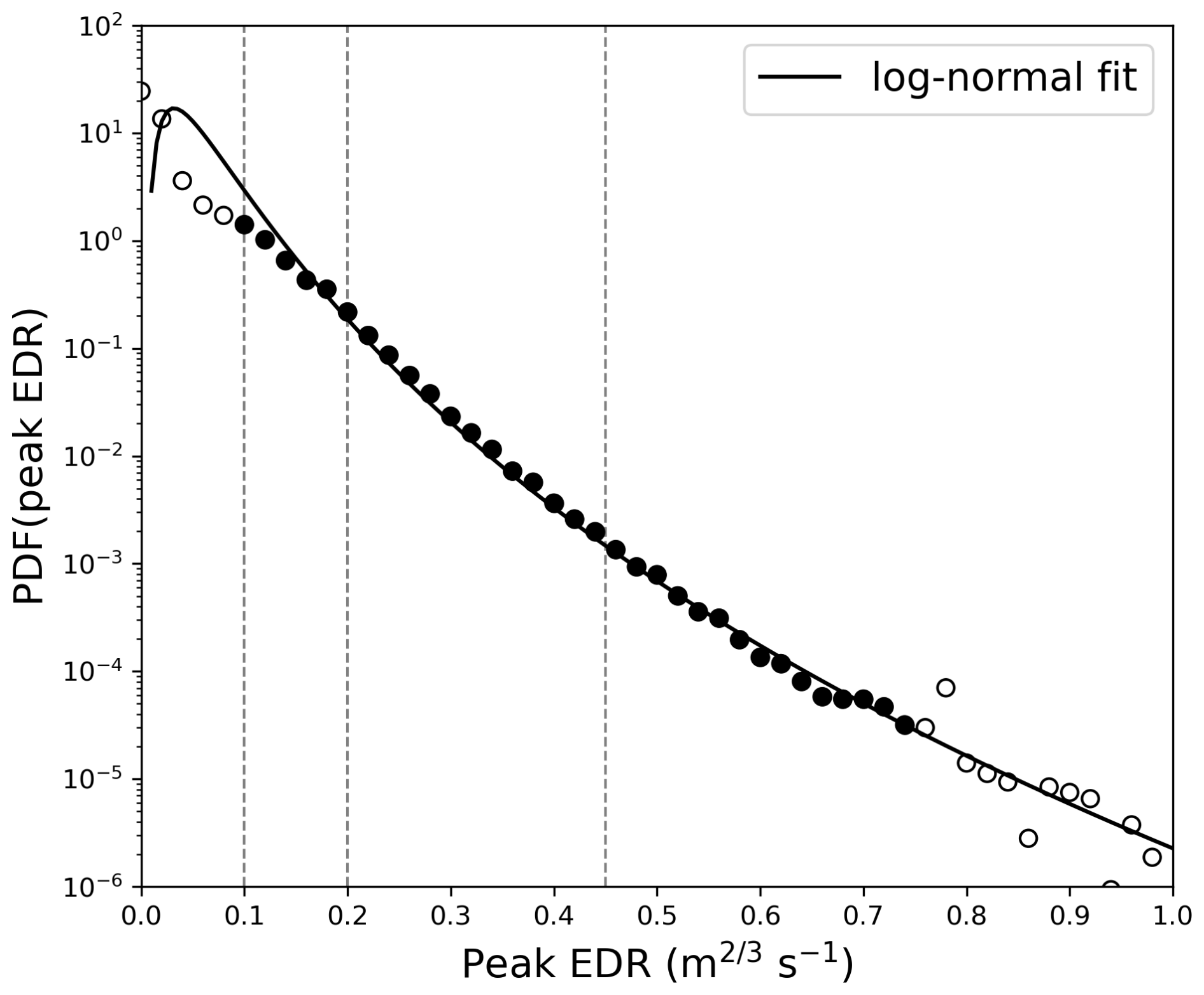
Figure A1 Probability density function of peak EDR (circles) and the lognormal fit (line) for the processed IATA Turbulence Aware data. The filled circles indicate bins included in the lognormal fit while the open circles indicate bins excluded from the fit (see text for details). The dashed vertical lines show the EDR threshold values of 0.1, 0.2, and 0.45, for light, moderate, and severe turbulence as stated in ICAO (2018).

The quality of the data is further checked by comparing the probability density function (PDF) of the peak EDR reports to published results of Sharman et al. (2014) (their Fig. 10b). A lognormal distribution is fitted to the binned peak EDR data (0.02 m${}^{\mathrm{2}/\mathrm{3}}$ s⁻¹ bin width) using the same method as in Sharman et al. (2014) and the result is shown in Fig. A1 (only values from 0.09 to 0.75 m${}^{\mathrm{2}/\mathrm{3}}$ s⁻¹ are used for fitting due to expected noise or low sample sizes). The peak EDR data fits well to the lognormal PDF and the fitting parameters give the mean logarithm of peak EDR $\langle \ln \left({\mathit{ϵ}}^{\mathrm{1}/\mathrm{3}}\right)\rangle$ = −3.076 and the standard deviation of logarithm of peak EDR ${\mathit{\sigma }}_{\ln {\mathit{ϵ}}^{\mathrm{1}/\mathrm{3}}}$ = 0.614. These values are comparable to those obtained from the DAL737 dataset in Sharman et al. (2014), which are −2.85 and 0.571 respectively. A later study by Sharman and Pearson (2017) suggested that the two parameters have values of −2.953 and 0.602 respectively for data obtained within 20 000 and 45 000 ft, which are also consistent with the IATA dataset.

A2 Turbulence event identification

The DBSCAN (Ester et al., 1996) algorithm is chosen for the identification of turbulence events. The algorithm is density-based, which naturally connects to the purpose of selecting well-sampled events. Also, it is suitable for turbulence event identification as the number of clusters is not predefined and data points can be assigned as noise. The two parameters required by the algorithm are the neighbourhood radius ϵ and the minimum number of points N. A data point is said to be a core point if there are at least N points within its neighbourhood with a radius of ϵ. Starting from a core point, a cluster is formed by searching recursively in the neighbourhood for other core points, until all core points and their non-core point neighbours are identified. Data points that do not belong to any cluster are defined as noise. This process is also deterministic and is favourable for this application.

To cluster the turbulence reports into spatially and temporally coherent events, the horizontal distance and the separation in time are normalised by their typical scales L and T respectively. The horizontal scale of a weather feature-related turbulence event is expected to be on the order of 100 km while the time scale is on the order of 10 min up to 1 h. As additional aircraft reports will be triggered in a turbulent condition with 1 min intervals, the number of reports by an aircraft due to one turbulence patch should be in the order of 10 reports. However, since pilots try to get out of turbulent conditions as soon as possible, the number should be lower per aircraft. Therefore, a set of length scales and time scales are tested with N = 5 or N = 10. The resultant numbers of events (ncluster) and discarded reports (nnoise) are assessed (Fig. S5, with ϵ fixed at 1) and they should not be highly sensitive to the set of parameters chosen. The setting with a length scale L being 250 km and a time scale T being 20 min (1200 s) generates the most reasonable results with N = 10 and is therefore employed in this study. Each identified event hence has at least a density of 10 turbulent reports within a circle with 250 km radius and in a time window of 40 min (doubled as 20 min is the “radius”). In total, 5867 events are identified over the globe (5780 in the Northern Hemisphere), with an average number of 22.8 reports per event and an average duration of 39.1 min.

A3 Clear-air condition classification

As the EDR reports do not indicate whether the aircraft is in clear-air conditions or not, additional observational data is needed to determine the condition accompanying the report. Infra-red brightness temperature measured by satellite is utilised to estimate the cloud top temperature, which allows a comparison with the air temperature measured by the aircraft. Assuming temperature is decreasing with height in the troposphere (and relatively constant in the lower stratosphere), an air temperature lower than the cloud top temperature would indicate that the aircraft is cruising at an altitude above the cloud top. While there might be inversions, this should most likely lead to identifying reports that are above cloud top as below cloud top, but not likely to cause below cloud top reports to be identified as above cloud top (as the cloud has to be above the inversion).

The satellite data, which originate from the National Centers for Environmental Prediction (NCEP) (Janowiak et al., 2017), contain merged infra-red brightness temperature from European, Japanese, and American geostationary satellites. Together they cover a global domain from 60° S to 60° N at 4 km resolution. The satellite data has a temporal resolution of 30 min and the cloud top temperature is estimated by interpolating the brightness temperature at the nearest time step to the location of the aircraft. The cloud top and air temperatures are then compared. To eliminate the potential measurement error from aircraft, the air temperature in ERA5 reanalysis is also included in the comparison, which is obtained by interpolation to the aircraft location using the data at the nearest hour. If both the aircraft and reanalysis air temperatures are lower than the cloud top temperature, the report is said to be in clear-air condition. In contrast, if both are higher than the cloud top temperature, the report is said to be in-cloud. All other cases, i.e. missing data or cloud top temperature being in between the reanalysis and aircraft air temperatures, are termed “undefined”.

An event is classified into “predominantly clear-air” and “in-cloud” according to the classes of its constituent reports. If more than half of the reports (excluding “undefined” reports) are “clear-air”, the event is termed “predominantly clear-air”. If it is in the opposite case, the event is termed “in-cloud”. The only exceptions are events that have all their reports classified as “undefined” and are termed “undefined”. According to this classification scheme, 4880 out of the 5780 events in the Northern Hemisphere are “predominantly clear-air”, 846 are “in-cloud” and 54 are “undefined”.

For grid point EDR, a grid point is considered “clear-air” if the air temperature in ERA5 reanalysis is lower than the corresponding remapped brightness temperature at the grid point. If the air temperature from reanalysis is higher, the grid point is considered “in-cloud”. For grid points that have at least one assigned EDR report, around 95.4 % are considered “clear-air”.