Resolution dependence and biases in cold and warm frontal heavy precipitation over Europe in CMIP6 and EURO-CORDEX models

Atmospheric cold and warm fronts are a major driver of heavy precipitation over Europe. To assess future changes in extreme weather, it is therefore essential to understand how frontal systems respond to a warming climate. This requires the analysis of climate model projections. A crucial first step is a process-based evaluation of frontal dynamics in present-day simulations, as this increases confidence in the models and the reliability of their future projections.

In this study, we compare the representation of frontal frequencies, frontal heavy precipitation, and frontal structure in the CMIP6 and EURO-CORDEX ensembles, using ERA5 as a reference. To assess the added value of higher resolution, we analyze the models on their native grids and compare them with ERA5 data remapped to similar resolutions.

We found that all models exhibit substantial biases in frontal frequencies and associated heavy precipitation, which are possibly related to storm-track position biases and an inadequate representation of land–atmosphere interactions. Warm frontal precipitation is generally better captured than cold frontal precipitation. Increasing model resolution leads to significant improvements for cold frontal biases, whereas warm frontal biases remain largely unaffected. The analysis of frontal structures supports this interpretation: while synoptic-scale conditions are well represented across models, mesoscale gradients and circulation patterns exhibit a pronounced sensitivity to grid spacing. Because warm fronts extend over larger horizontal scales, they are already reasonably well simulated at coarse resolution. Cold fronts, by contrast, are governed by smaller-scale processes and therefore show notable improvements at higher resolution.

These findings provide an important step toward evaluating climate models in their ability to simulate impactful weather phenomena. While warm frontal precipitation appears robust across model resolutions, reliable simulations of cold fronts require higher-resolution models to adequately capture their dynamics and associated heavy precipitation.

1 Introduction

Extreme weather in the mid-latitudes is frequently caused by atmospheric fronts (Catto et al., 2012). Cold fronts are typically associated with strong wind gusts and intense short-duration precipitation, often leading to localized flooding. In contrast, warm frontal precipitation is generally more widespread but less intense, potentially causing flooding across larger catchments.

Numerous studies have demonstrated the connection between frontal systems and extremes in Europe. For example, half of all hail events in Switzerland have been linked to cold fronts (Schemm et al., 2016), while in Germany convective cells are twice as likely to form in the vicinity of cold fronts during the warm season (Pacey et al., 2023). The proportion of precipitation associated with all fronts over Europe range from 30 %–80 %, with strong regional and seasonal differences (Catto et al., 2012; Hénin et al., 2019; Rüdisühli et al., 2020). For heavy precipitation events, the estimated contribution increases to 60 %–90 % (Catto and Pfahl, 2013).

Given their central role in generating high-impact weather, future changes in frontal systems need to be studied in detail to increase confidence in projections of extremes (Marotzke et al., 2017; Collins et al., 2018). Therefore, it is essential to first assess how well climate models represent atmospheric fronts in the current climate and, based on these process-based evaluations, assess projections of extremes (IPCC, 2023).

In our previous work, we examined the drivers of cold frontal extremes (Schaffer et al., 2024) and analyzed the cold frontal life cycle in reanalysis data (Lichtenegger et al., 2025). Building on these findings and methodologies, we now assess the performance of a range of climate models. Catto et al. (2014) were the first to evaluate front frequencies in climate models under both present and future conditions, finding good agreement between ERA-Interim and CMIP5 datasets. They also projected decreases in both the frequency and intensity of fronts across many regions under the RCP8.5 scenario.

Here, we evaluate the Coupled Model Intercomparison Project Phase 6 (CMIP6) dataset (Eyring et al., 2016), together with the latest generation of the European Centre for Medium-Range Weather Forecasts atmospheric reanalysis (ERA5) (Hersbach et al., 2020) as a reference. Our analysis extends previous work by investigating the added value of higher-resolution models in simulating atmospheric fronts and by quantifying biases in the associated heavy precipitation. To explore a broader range of model resolutions, we further analyze the Coordinated Downscaling Experiment over Europe (EURO-CORDEX) dataset (Jacob et al., 2014). Extending the analysis from GCMs to RCMs enables us to evaluate the benefits of resolving fronts at the 10 km-scale. A key focus is to link potential biases in heavy precipitation to deficiencies in the representation of the frontal structure and processes. To this end, for the first time, we perform an analysis of frontal cross-sections in study based on climate model simulations.

2 Data

We analyze 15 GCMs from the CMIP6 ensemble (Eyring et al., 2016), 15 RCM simulations from EURO-CORDEX (Jacob et al., 2014), and the ERA5 reanalysis dataset (Hersbach et al., 2020) for the period 1970–2005. Within the EURO-CORDEX ensemble, three different RCMs are each driven by between four and six GCMs. All simulations providing the necessary 6-hourly, three-dimensional fields of temperature, humidity, wind, geopotential height, and precipitation from the ensembles have been selected. A complete list of all models used is provided in Table 1.

Table 1 Overview of all datasets used in this study, including horizontal resolution, number of available pressure levels and associated sub-ensemble classification.

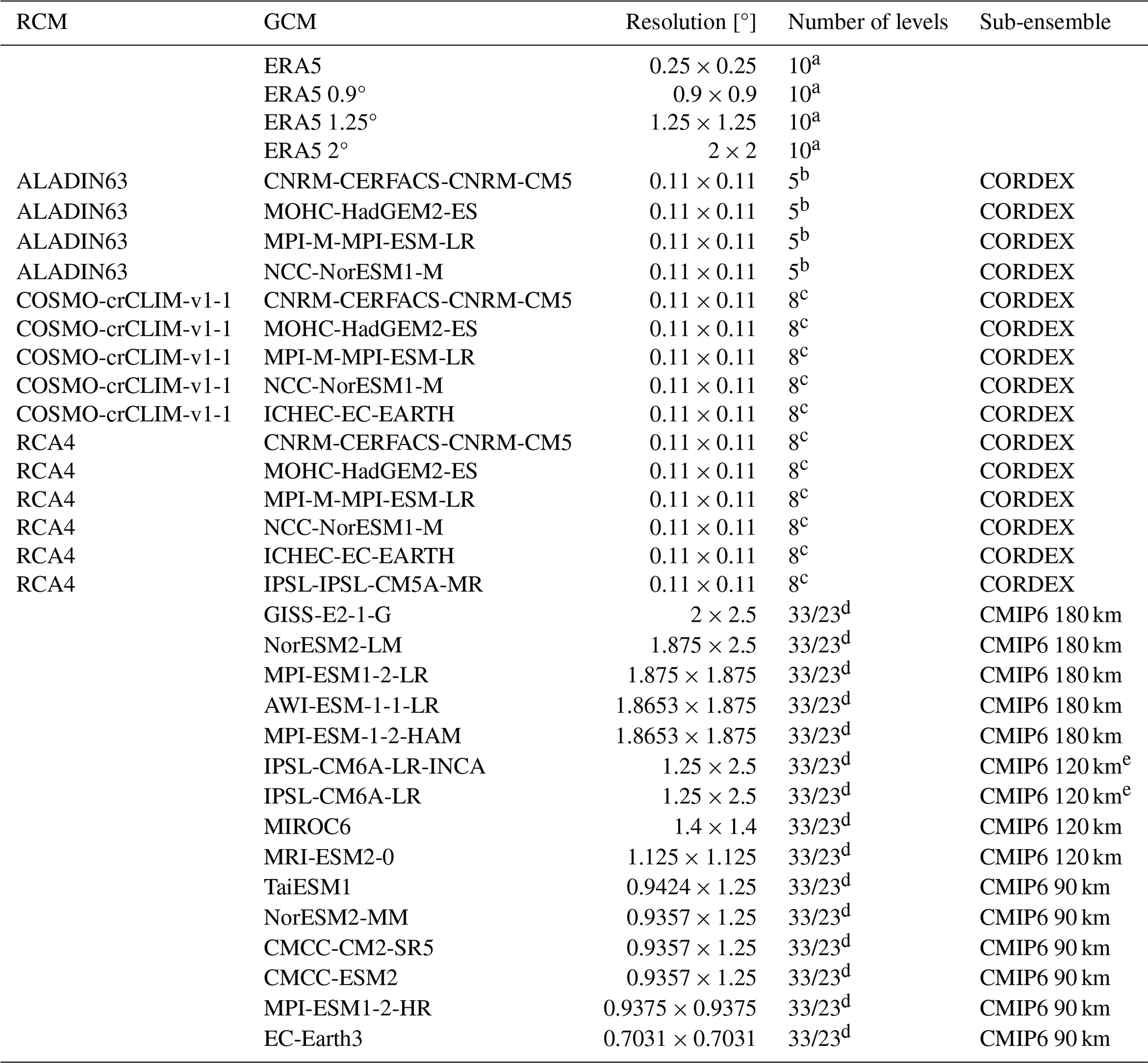
^a 1000, 925, 900, 850, 700, 600, 500, 400, 300, 200 hPa.
^b 925, 850, 700, 500, 200 hPa.
^c 925, 850, 700, 600, 500, 400, 300, 200 hPa.
^d 1000–200 (25 hPa steps), with 10 levels missing geopotential data (725, 675, 625, 575, 525, 475, 425, 375, 325, 275 hPa).
^e The IPSL model is included in the CMIP6 120 km sub-ensemble because its results aligned more closely with that group than with others.

Resolution effect

To evaluate the added value of higher spatial resolution, all analysis is performed on the native model grids. However, the analysis itself is inherently impacted by resolution because coarser grids introduce smoothing to all physical fields. The averaging not only reduces the representation of smaller-scale physics, but for precipitation fields it potentially hides its extremeness. To improve consistency, all data are spectrally filtered prior to the analysis to reduce small-scale variability. However, the horizontal grid resolution continues to strongly impact the results. To illustrate this effect, a comparison of front frequencies in ERA5 compared with ERA5 remapped to three coarser resolutions (2, 1.25 and 0.9°) is shown in Fig. 1. The error introduced by resolution is of the same order as the model biases. Previous studies avoided potential methodological biases from resolution disparities by remapping all data to the same coarse grid (e.g., Catto et al., 2014; King et al., 2024).

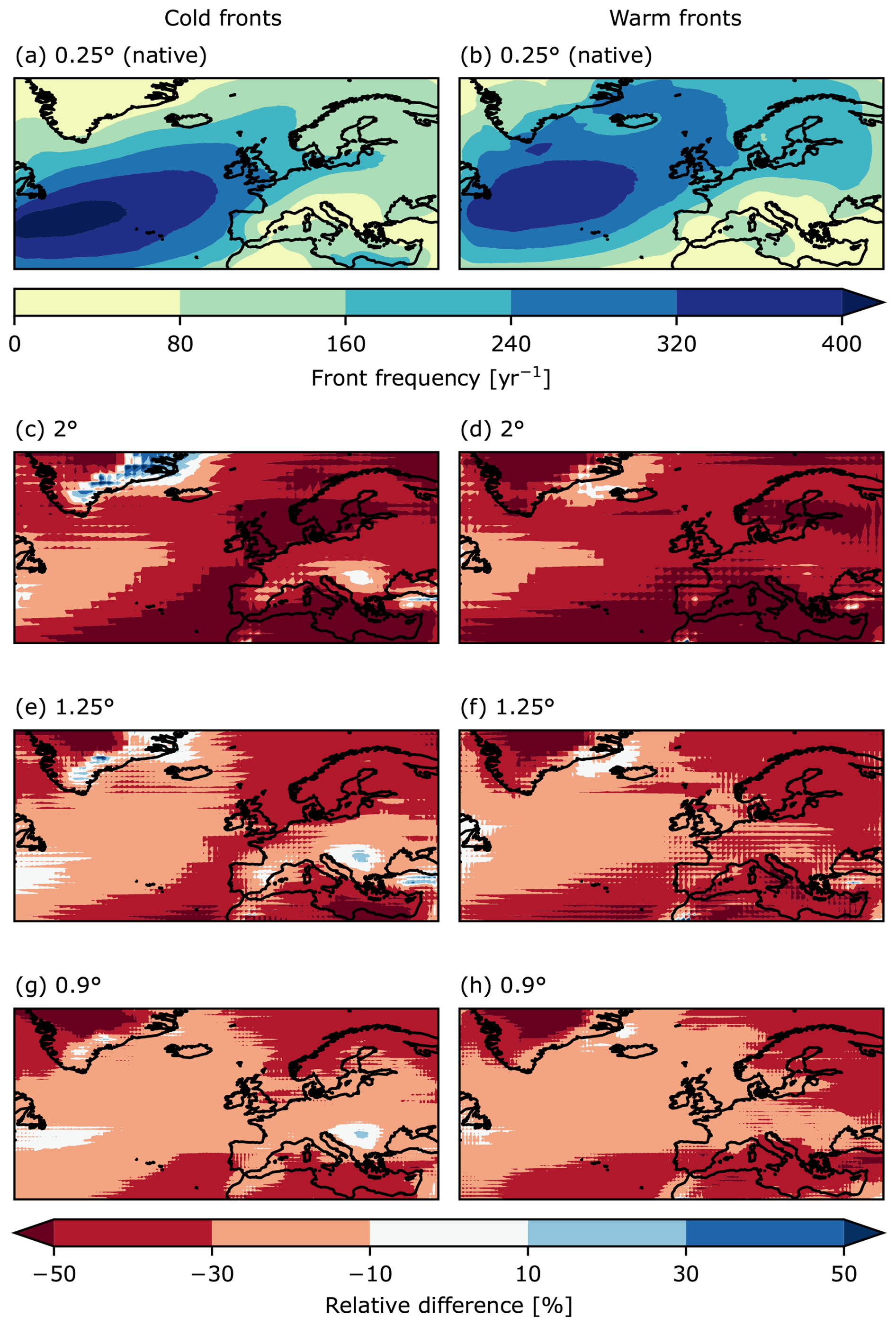
Figure 1 Front frequency in ERA5 at (a, b) 0.25°, (c, d) 2°, (e, f) 1.25°, and (g, h) 0.9° resolution for (a, c, e, g) cold and (b, d, f, h) warm fronts. Panels (a) and (b) show the number of timesteps with front occurrence per year while panels (c)–(h) depict the relative difference compared to native-resolution ERA5.

In this study, we minimize methodological biases related to resolution differences, while assessing the added value of higher resolutions, by following a similar approach to that described in Volosciuk et al. (2015): prior to the front detection and analysis, ERA5 is remapped to the three aforementioned coarser resolutions of 2° × 2°, 1.25° × 1.25°, and 0.9° × 0.9°. Based on their resolution, the CMIP6 models are classified into three sub-ensembles: coarse (180 km), mid (120 km), and high resolution (90 km). These sub-ensembles are compared with the remapped ERA5 data with the closest mean horizontal grid spacing. This step minimizes errors arising from resolution differences when comparing datasets. The EURO-CORDEX models are analyzed similarly on the native grid and evaluated against the native ERA5 data. Because ERA5 has a coarser grid than EURO-CORDEX, some methodological bias is introduced to this analysis. For comparison and plotting purposes, all results are remapped conservatively to a uniform 0.25° × 0.25° resolution.

The mid-resolution CMIP6 sub-ensemble consists of four models, of which two are from the IPSL. Unlike the other models, these have distinct latitudinal and longitudinal grid sizes. As a consequence, their results align best with those of mid-resolution CMIP6 models. For that reason, they are classified with this sub-ensemble. Because half of the sub-ensemble is made up of IPSL models, they have a strong impact on the results. These effects are mentioned in the result section and are discussed in more detail in the Supplement, but the evaluation of specific causes is beyond the scope of this study.

3 Methods

The methods applied in this study closely follow those described in Schaffer et al. (2024). An overview of the approach, including all modifications, is provided here. For a more detailed explanation, we refer the reader to the previous study.

3.1 Front detection

The front detection scheme employed in this study follows established approaches in the literature (e.g., Hewson, 1998; Jenkner et al., 2009), in which regions of strong thermal gradients are identified and a wind-based threshold is subsequently applied. In detail, fronts are detected by applying a threshold to the smoothed equivalent potential temperature gradient (∇θ_e) field at 850 hPa. The threshold is defined as the seasonal spatial mean plus one standard deviation of ∇θ_e over the North Atlantic region (20–12° W, 40–58° N) for the period 1970–2005, computed separately for each model. This region was selected because it is covered by all datasets, lies within the climatological storm track, and is free from orographic interference.

The final frontal points are identified as local maxima in ∇θ_e where the Thermal Front Parameter (TFP) is closest to zero. TFP is defined as:

$$\begin{array}{}\text{(1)}& \text{TFP}=-\mathrm{\nabla }\left|\mathrm{\nabla }{\mathit{\theta }}_{\mathrm{e}}\right|\cdot {\displaystyle \frac{\mathrm{\nabla }{\mathit{\theta }}_{\mathrm{e}}}{\left|\mathrm{\nabla }{\mathit{\theta }}_{\mathrm{e}}\right|}}\end{array}$$

and measures the rate of change of ∇θ_e in direction of the gradient. Based on the cross-frontal wind speed (u_f), these points are classified into cold fronts (u_f > 1.5 m s⁻¹) and warm fronts (u_f < −1.5 m s⁻¹). Points with weaker u_f are excluded to ensure that only mobile synoptic-scale fronts are retained. Connected frontal points are grouped into contiguous frontal objects. To exclude non-synoptic features, a minimum length threshold of 500 km is applied.

The detected fronts still contain some unwanted objects. Along coasts and mountain ranges (e.g., the Norwegian coast, the western Balkan coast), humidity differences can lead to the detection of spurious air mass boundaries as cold fronts, which are not relevant for our analysis. We remove these objects by comparing the angles of the ∇θ_e and geopotential height gradient vectors. In synoptic-scale cold fronts, these vectors typically point in the same direction. By applying a threshold on the absolute angle difference of greater than 120°, we not only remove non-frontal objects but also exclude back-bent fronts from the cold front analysis. Similarly, strong humidity gradients at the warm-side boundary of the warm conveyor belt are often falsely detected as warm fronts. To filter these objects, we require a positive potential temperature difference between points located 300 km ahead and 300 km behind of the warm frontal points at 850 hPa. Because the warm conveyor belt generally exhibits higher equivalent potential temperatures but lower potential temperatures than the air farther ahead of the cold front, the criterion effectively removes many of these unwanted detections.

3.2 Frontal frequency and precipitation

After the detection, the frontal data consisting of grid points labeled either 1 or −1 depending on the front type. In this state, it is not possible to compare the frequencies of the different models due to the dependence of the frontal width on the resolution of the grid. Using a grid-factor (e.g. number of high-resolution grid points per low-resolution grid point) is also not possible, because of the varying extent and curvature of fronts in higher resolution data. To make the frequencies comparable, we define a frontal area as a circular region with a 300 km radius centered on each frontal point. The resulting objects have a consistent physical width of 600 km across all datasets, independent of their resolution. These areas are masked and subsequently summed up to estimate the frequency of fronts.

Precipitation is considered frontal if it occurs within the defined frontal area. We further classify precipitation as heavy if the 6-hourly total exceeds the 99.5th percentile at each grid point, corresponding to a return period of 50 d. Following Hénin et al. (2019), precipitation is split between cold and warm frontal when it falls within the 300 km radius of both front types. In such cases, precipitation is partitioned proportionally to the number of grid points associated with each front type (e.g., if 6 cold and 4 warm frontal points are within the radius, 60 % of the precipitation amount is classified as cold and 40 % as warm frontal). By summing the total and frontal heavy precipitation, we then compute the fraction associated with each front type.

3.3 Frontal composites

To construct the frontal composites, we apply a multi-step procedure designed to capture the typical structures of intense frontal systems. First, we determine the precipitation associated with each frontal object by focusing on the most active 200 km segment of the front. To do so, we calculate the number of frontal grid points corresponding to a length of approximately 200 km based on the model resolution. All frontal points within a given object are then ranked by their standardized precipitation values (normalized by its mean and standard deviation), and the top-ranked points that together represent about 200 km of frontal length are selected. The precipitation of the frontal object is defined as the mean precipitation of these selected frontal points. This approach ensures that the composites are based on the most intense and meteorologically relevant parts of each front, independent of variations in model resolution or front length.

To avoid sampling of the same frontal system in multiple time steps, only one front per 24 h period is included in the analysis. From the resulting objects, the top 10 %, ranked by standardized precipitation, are then used to generate the composites. The regions used to evaluate these fronts are defined as: Northwestern Europe (NWEUR, 48–61° N, 12° E–3° W), Southwestern Europe (SWEUR, 36–48° N, 11° E–4° W), and Central Europe (CEUR, 48–58° N, 3–25° W). These regions are selected due to their high front frequency and fraction of heavy frontal precipitation. To ensure a more focused and comprehensive analysis, we combine the frontal events from all three regions and seasons into a single dataset, from which composites are calculated.

The frontal cross-section composites are generated by extracting 1200 × 1200 km atmospheric fields centered on the frontal objects. The position of each frontal object is determined by the frontal point with the median standardized precipitation within the aforementioned top-ranked frontal points of an object. The median frontal point is chosen to minimize the number of cross-sections that are affected by the occlusion point. The extracted fields are rotated into the cross-frontal direction and bilinearly interpolated to a common set of standard pressure levels (925–200 hPa in 25 hPa steps) before computing the composites. While differences in the native vertical resolution could affect the representation of the frontal structure, the resulting composites are smooth, suggesting that interpolation and vertical resolution differences have only a minor impact. To analyze composites of front-relative circulation, the dynamic variable fields are separated into synoptic and mesoscale components using a spectral filter. The filter settings are 1500 km low pass and 500 km standard deviation of the transfer function, ensuring wavelengths larger than 1000 km make up the synoptic-scale and smaller wavelengths the meso-scale. This step is performed for every frontal event prior to the calculation of the composites.

4 Results

4.1 Frontal frequency

Before evaluating model biases in front frequency and the associated heavy precipitation, we want to give a detailed look at the effect of horizontal resolution on the detection for ERA5. To this end we compare ERA5 on the native grid to the three coarsened remaps, which will act as a reference to the model data. Figure 1a–b show the absolute front frequency based on native-resolution ERA5, which is qualitatively consistent with the hourly frequencies reported in Schaffer et al. (2024). Quantitative differences arise from the differing temporal resolutions, as well as from the adapted frequency evaluation methodology. In Fig. 1c–h, the previously discussed strong relationship between grid resolution and front frequency is evident. The coarsest resolution data (2°) show over 50 % fewer cold and warm fronts across large parts of the study domain. The bias is substantially reduced at higher resolutions (1.25 and 0.9°). In some regions, higher frequencies in the remap data compared to the native data can be observed (e.g., along the coast of Greenland, the Balkans, Anatolia). Positive resolution biases in these areas are likely due to the influence of orography, which becomes increasingly smoothed at lower resolutions, thereby enabling more continuous front detection in mountainous regions.

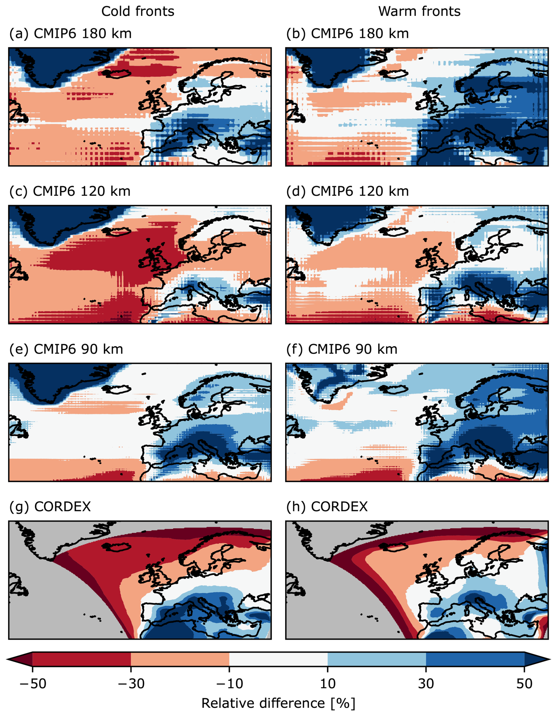
Figure 2 Relative front frequency bias of the (a, b) coarse CMIP6, (c, d) mid CMIP6, (e, f) fine CMIP6 and (g, h) CORDEX models compared to the respective ERA5 remap for (a, c, e, g) cold and (b, d, f, h) warm fronts. Grey indicate areas outside the EURO-CORDEX domain. The pronounced negative biases of CORDEX near the northern and western domain boundaries are caused by the 500 km minimum front length threshold, which excludes valid fronts that extend beyond the domain boundaries.

Model biases in frontal precipitation may be explained primarily by underlying frontal frequency biases. Thus, in the following the relative front frequency biases of the different model ensembles are shown in Fig. 2. In general, the models simulate lower front frequencies over the North Atlantic and higher frequencies over continental Europe. Notably, positive biases are found over orographically complex regions such as the Alps and Anatolia, as well as on the leeward sides of major mountain ranges (e.g., the Iberian Peninsula and Scandinavia). These patterns are consistent across all model resolutions and do not improve when mountains are represented in more detail, suggesting that the smoothed orography is not the main cause. A reduction of boundary-layer friction in the models could intensify frontal circulation and enhance frontogenesis, which would strengthen ∇θ_e and could increase the likelihood of detecting fronts.

Looking more into the individual sub-ensemble results, it can be seen that CORDEX exhibits a clear positive bias over southern Europe and a negative bias over northern Europe for cold and warm fronts alike (Fig. 2g–h). Previous studies have documented an overly zonal storm track in CMIP5 simulations (Priestley et al., 2020; Harvey et al., 2020), which may contribute to these regional differences in the EURO-CORDEX ensemble. A similar storm track bias may also influence CMIP6 simulations, although the same studies have indicated that the latest CMIP version has improved their performance in this regard. The elevated front frequencies in a zonal band over the North Atlantic (approximately 43–47° N) in CMIP6 models may still be the result of the residual error in the storm track position.

The effect of these biases can be seen in both cold and warm frontal frequencies. Comparing cold and warm fronts in more detail reveals that warm fronts are generally detected more frequently in the models. This overall bias is consistent across all model resolutions. Over the North Atlantic, they show smaller differences compared to ERA5, whereas over continental Europe, the differences are larger.

Following the bias analysis, we investigate the effect of mean horizontal resolution on front frequencies across specific regions, as defined in Fig. A1. The regression between model resolution and front frequency is shown in Fig. 3 for cold (a) and warm (b) fronts. Across all datasets, a strong negative relationship is found: smaller grid sizes are associated with higher front frequencies. Increasing the resolution by 100 km results in the detection of approximately 15–60 additional fronts per year within each region, corresponding to an increase of 8 %–46 %. Cold fronts show slightly steeper regression slopes, ranging from 16–60 fronts per year per 100 km (12 %–46 %), compared to warm fronts, which range from 17–50 fronts per year per 100 km (8 %–34 %). Overall, these results suggest that cold frontal frequencies exhibit a stronger sensitivity to horizontal resolution compared to warm fronts.

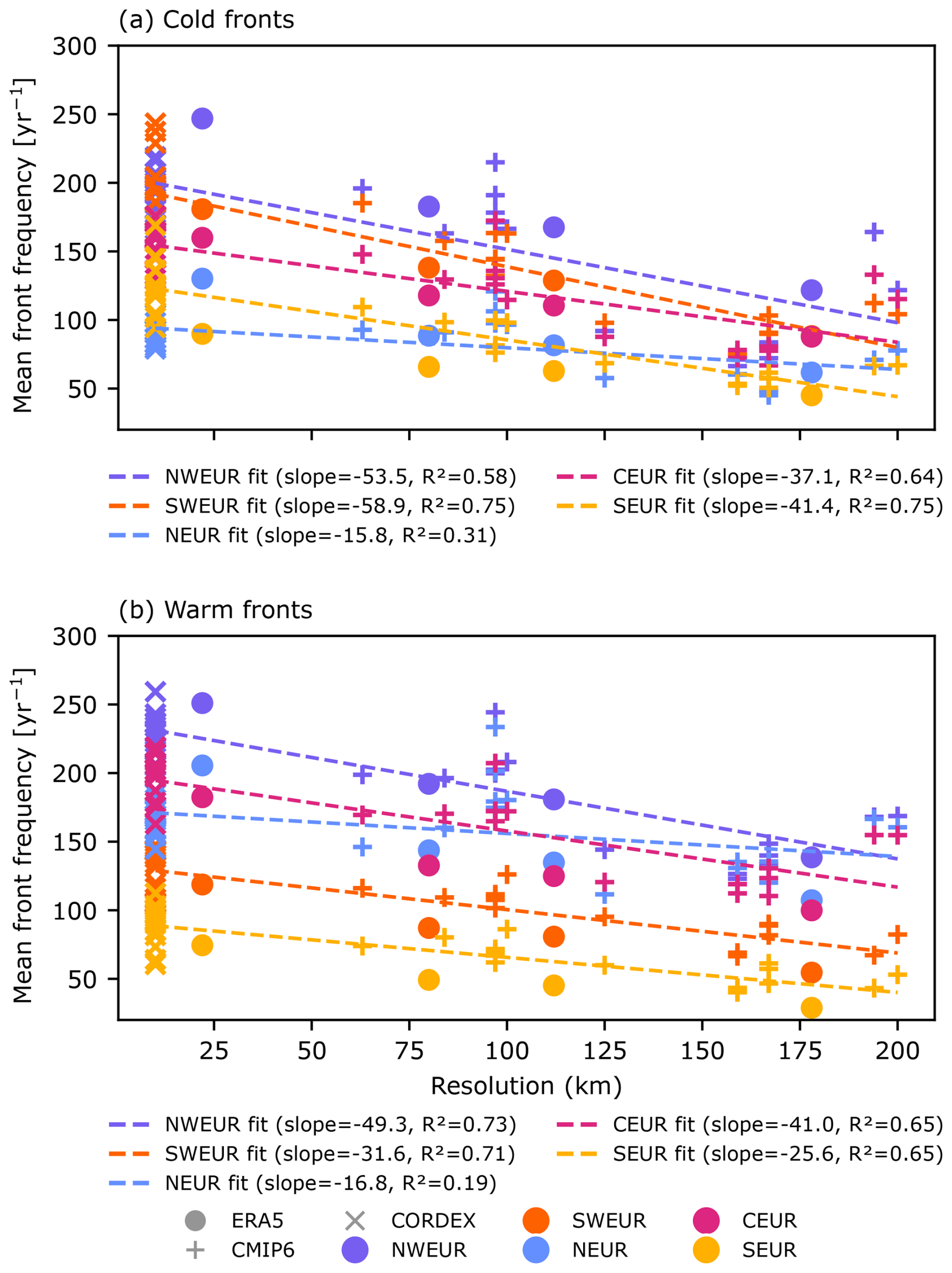
Figure 3 Regression of model resolution with mean front frequency over selected regions for (a) cold and (b) warm fronts. The colored (•) indicate ERA5 and its remaps, (x) CMIP6 and (+) CORDEX models. The colored dashed lines show the regression lines, with the values of the slopes and regression coefficients (r²) in the legends. The colors indicate the regions. The y axis shows the mean front frequency values. The resolution values depicted on the x axis are equal to the geometric mean horizontal grid lengths at 50° N.

The north-south bias in the CORDEX models, which we previously linked to the storm track position (Fig. 2g–h), is also evident in the regression results. The NEUR and NWEUR region have lower mean front frequency values than expected from the regression. For the NEUR region the strong domain boundary error may also have an impact. When CORDEX is excluded, the relationship becomes stronger, with the steepness of the slope increasing from 54 and 16 (49 and 17) (Fig. 3) to 86 and 40 (76 and 36) (Fig. S1 in the Supplement) additional fronts per 100 km for cold (warm) fronts, for NWEUR and NEUR respectively. Furthermore, the slopes for SEUR decrease from 41 (26) (Fig. 3) to 29 (22) (Fig. S1) fronts per 100 km for cold (warm) fronts, indicating that CORDEX tends to underestimate frontal frequencies in northern regions while overestimating them in southern Europe.

These results confirm and extend the resolution-related findings from Fig. 1 to the full ensemble of climate model data. The resolution dependence of front detection is a key factor in evaluating both the bias in frontal heavy precipitation and the potential resolution effects on it.

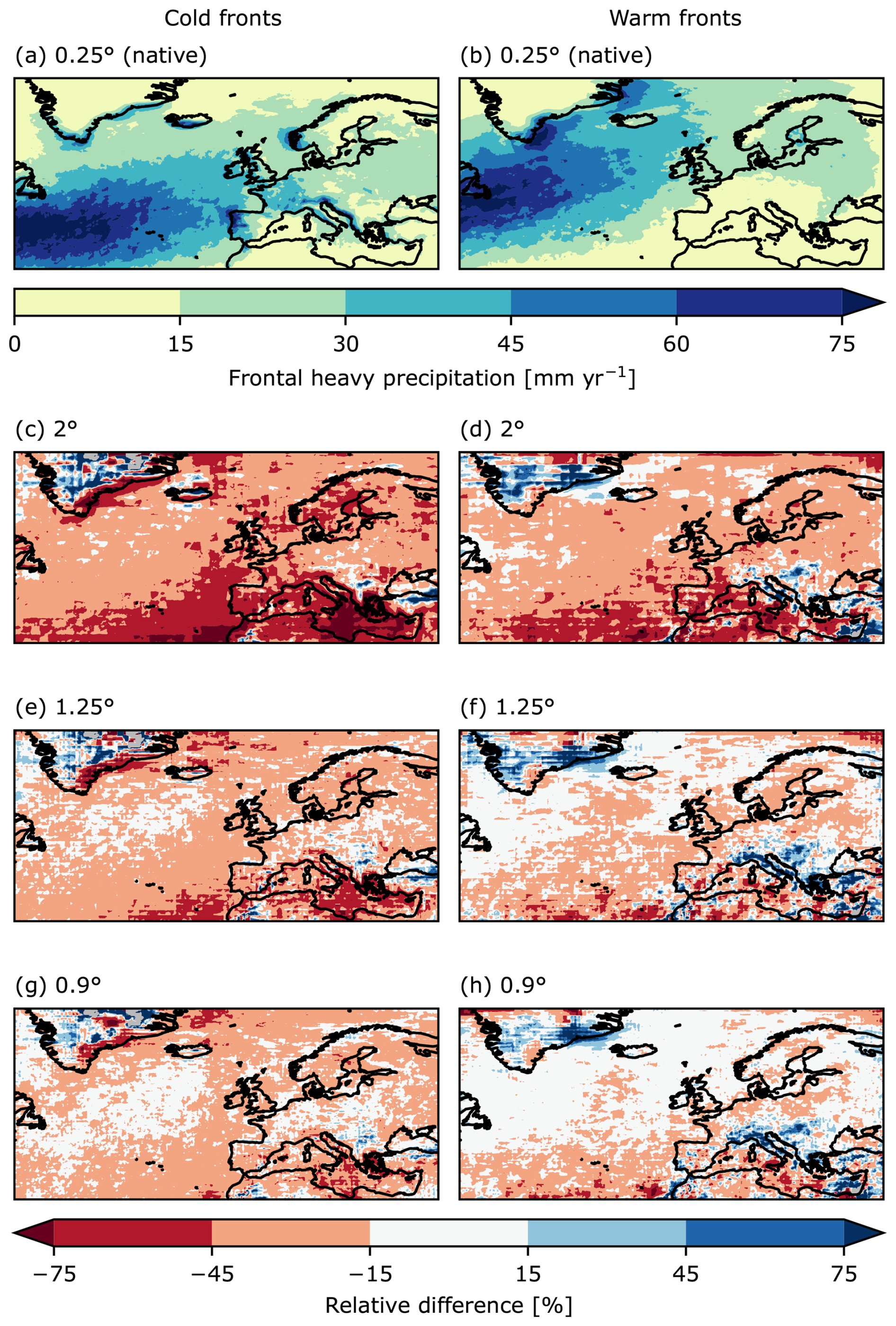
Figure 4 Same as Fig. 1, but for frontal heavy precipitation.

4.2 Frontal precipitation

Similarly to the front frequency analysis, the effect of resolution on frontal heavy precipitation (as defined in Sect. 3.2) is the first important step to evaluate biases. Differences between the remapped ERA5 data and the native resolution data again reveal a strong dependence on grid size. The coarsest grid shows a reduction of 15 %–75 % in frontal heavy precipitation (Fig. 4c–d). Similar to the pattern observed in the front frequency analysis, the bias decreases with increasing resolution (Fig. 4e–f). The largest negative differences appear in the southern part of the study domain, which also exhibit strong biases in front frequency, while areas with positive differences in frontal precipitation tend to coincide with regions where more fronts are detected. A similar resolution dependence is found for the total amount of heavy precipitation (i.e., not only frontal), which decreases on coarser grids due to a dampening of the tail of the precipitation distribution (Fig. S2).

When comparing heavy precipitation associated with each front type, warm fronts exhibit smaller deviations from the native-resolution data than cold fronts. Part of this effect could be attributed to the fact that precipitation near the occlusion point tends to be classified more often as warm frontal in lower-resolution data. The likely reason is that smoother θ_e and wind fields in coarser grids shift the detected position of cold fronts farther from their intersection with warm fronts. Since high-intensity precipitation frequently occurs near the occlusion point, a larger fraction of precipitation may therefore be attributed to warm fronts in coarser-resolution data. However, the main cause is likely the broader area that warm frontal precipitation typically spans compared to the narrow cold frontal rain bands. It is therefore better represented at coarser resolutions. This finding highlights the importance of high-resolution GCMs for capturing the intensity of sub-daily cold frontal precipitation. Warm frontal precipitation, on the other hand, is shown to be less sensitive to grid size.

The model data similarly favor warm over cold frontal heavy precipitation. In Fig. 5, a general negative bias is evident for cold frontal precipitation, while a strong positive bias is seen for warm frontal precipitation. When both front categories are combined, the deviations from ERA5 are reduced to within ±15 % across most areas in CMIP6. The pronounced positive bias over the Mediterranean and northern Africa in the CORDEX ensemble is mainly driven by the increase in front frequency, likely linked to the aforementioned storm track bias. This interpretation is supported by the average precipitation per front bias, which is comparable to the other model ensembles (Fig. S3).

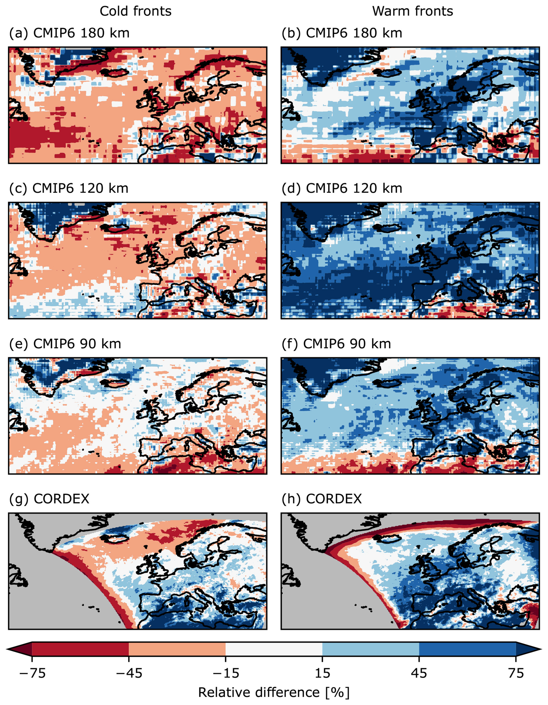
Figure 5 Same as Fig. 2, but for frontal heavy precipitation bias.

Once again, cold fronts seem to benefit from higher resolution in the GCMs: with decreasing grid size, the cold frontal precipitation bias is reduced across much of the study domain (Fig. 5a, c, e). The reduction suggests an improved representation of cold frontal processes and associated rainbands in higher-resolution simulations. In contrast, the warm frontal bias remains largely consistent across all sub-ensembles (Fig. 5b, d, f, h). Even over the Atlantic where warm front detection is substantially lower than in ERA5 (Fig. 2b, d, f, h), the models simulate more heavy precipitation associated with warm fronts compared to ERA5. The CMIP6 120 km sub-ensemble displays very high warm frontal precipitation over both the ocean and the continent. A detailed analysis of the constituent models of the sub-ensemble is presented in the Supplement (Fig. S4).

An analysis of the fraction of heavy precipitation associated with cold and warm fronts supports the conclusion, that mainly cold frontal precipitation benefits from higher resolutions (Fig. S5). In CMIP6, absolute heavy precipitation values increase with resolution, but the fraction only increases for cold fronts (i.e. the fraction difference to ERA5 decreases). The increase in warm frontal precipitation is driven by an increase in total heavy precipitation, related to the reduced grid averaging effect, not to an improved physical representation. However, better-resolved cold fronts benefit more strongly, highlighting the added value of finer grids.

To quantify this resolution effect more explicitly, we analyze the relationship between grid spacing and frontal heavy precipitation. Figure 6a illustrates the positive influence of resolution on cold frontal heavy precipitation. For every 100 km decrease in grid spacing, an average increase of 5–16 mm of heavy precipitation per year is detected per region. While this relationship may partly result from higher cold front frequencies at finer resolutions, an improved representation of smaller-scale frontal processes is also likely to contribute. Restricting the analysis to CMIP6 and ERA5 data further enhances the consistency and alignment of regional patterns (Fig. S6a).

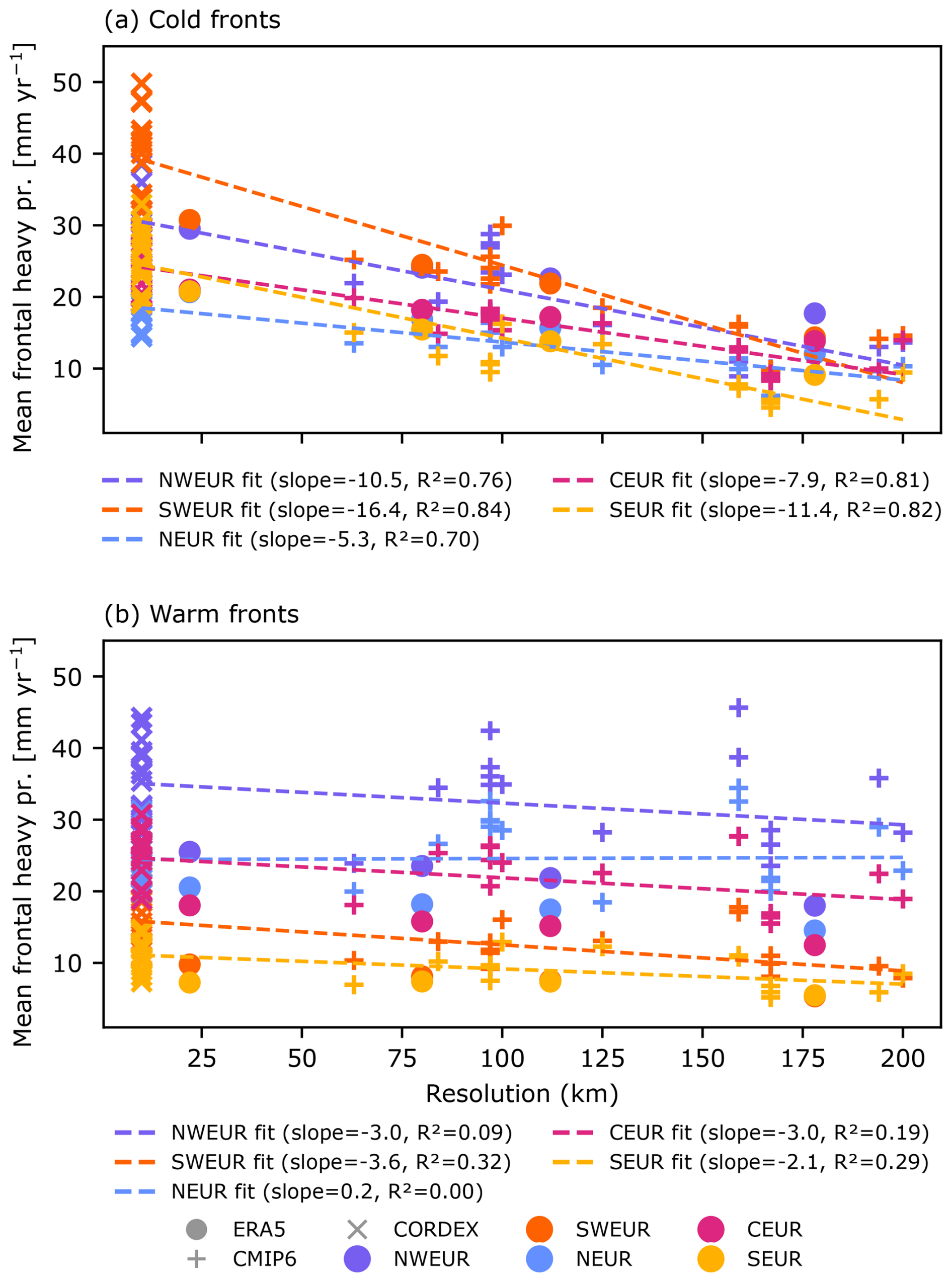
Figure 6 Same as Fig. 3, but showing the regression of model resolution with mean frontal heavy precipitation over selected regions.

In contrast, warm frontal precipitation shows only a weak negative correlation with resolution (Fig. 6b). When CORDEX models are excluded, this relationship disappears entirely (Fig. S6b), even though higher-resolution models detect warm fronts more frequently, as shown in Fig. 3b. This finding further supports the idea that warm frontal precipitation and associated rainbands are already well captured by current-generation GCMs.

4.3 Frontal composites

To understand why cold frontal heavy precipitation is particularly sensitive to model resolution, we examine the frontal structure and associated circulation patterns. Our goal is to identify structural differences across models that may explain the resolution–precipitation relationship observed in the previous section. For this purpose, we analyze cross-sections of composites of strong cold (Fig. 7) and warm fronts (Fig. 8). Note that these composites are based on fronts selected independently from those associated with the heavy precipitation discussed in the previous section, but by following the method described in Sect. 3.3.

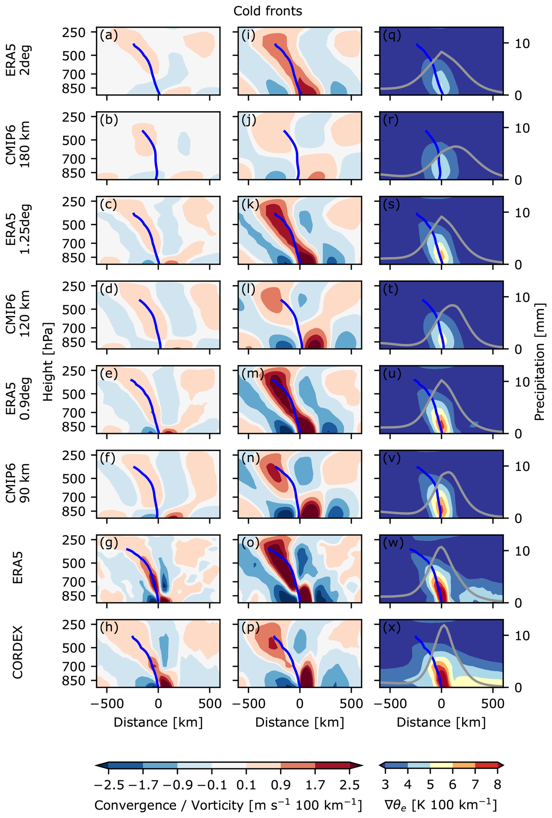
Figure 7 Cross-section composites of cold fronts. The x axis depicts the cross-frontal distance from 600 km behind to 600 km ahead of the detected front at 850 hPa. The y axis depicts the vertical pressure levels from 925–200 hPa and in panels (q)–(x) additionally the precipitation in mm. The filled contours display (a–h) mesoscale horizontal convergence in m s⁻¹ 100 km⁻¹, (i–p) mesoscale horizontal vorticity in m s⁻¹ 100 km⁻¹ and (q–x) ∇θ_e in K 100 km⁻¹. The contour in panels (q)–(x) illustrates the distribution of precipitation. Each panel row represents the composite of ERA5 or a sub-ensemble. The blue line represents the approximate mean position of the detected cold fronts based on the TFP zero contour.

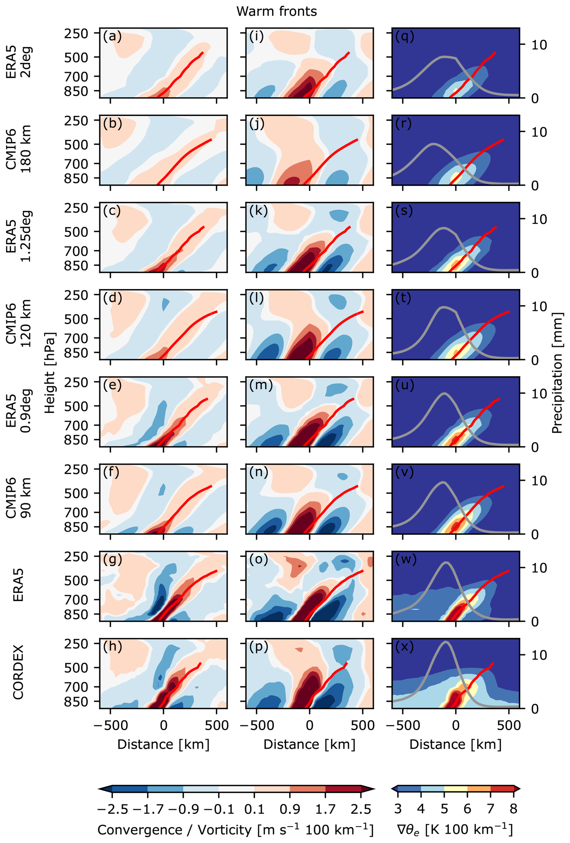
Figure 8 Same as 7, but for warm front composites. The red line represents the approximate mean position of the detected warm fronts.

At the large-scale, the composite fields of temperature, humidity (Figs. S7–S8), and circulation (Figs. S9–S10) show good agreement between ERA5 and all model ensembles. The large-scale convergence fields are smooth and similar across models, reflecting the fact that wavelengths longer than ∼ 1000 km are well represented even in coarse-resolution models. However, mesoscale gradients (Figs. 7q–x, 8q–x) and circulation features (Figs. 7a–p, 8a–p) display a pronounced sensitivity to horizontal resolution. Coarse-resolution models resolve very little variability at sub-synoptic scales, resulting in weak mesoscale convergence, whereas the large-scale fields remain unaffected. Consequently, in these models a comparatively larger fraction of the total circulation is contained in the large-scale component. Higher-resolution models capture sharper frontal gradients and enhanced mesoscale convergence, improving their representation of precipitation variability and allows models to better capture heavy precipitation events.

Overall, the cold (Fig. 7) and warm frontal structure (Fig. 8) is well captured across all models when differences in resolution are considered. Mesoscale circulations, however, show some biases. Vorticity in cold fronts (Fig. 7i–p) exhibits the biggest differences, with all CMIP6 sub-ensembles showing a split between the upper- and lower-level positive vorticity regions. In contrast, ERA5 has a continuous backwards-sloped area of high vorticity. This is due to the low-level jet position, which in CMIP6 on average is located further ahead of the cold front than in ERA5. The maximum vorticity is further approximately 20 % lower in all models, and the maximum convergence ranges from −30 % in coarse-resolution models to +30 % in CORDEX. Although these differences are evident, they do not indicate fundamental structural errors. Nevertheless, limited representation of small-scale dynamics by coarse models likely diminishes the intensity and organization of precipitation bands, a factor especially critical for cold frontal precipitation.

Comparing cold and warm fronts reveals systematic differences in precipitation characteristics (Figs. 7q–x, 8q–x). Warm fronts exhibit larger total precipitation in the composites, though not necessarily higher peak intensities, consistent with the warm front precipitation biases over Europe. Although total precipitation varies between models, there is no clear dependence on resolution. In contrast, for both cold and warm fronts, the distribution of precipitation narrows with increasing resolution, reflecting a higher ability of finer grids to resolve localized heavy precipitation.

Furthermore, the lower-level convergence and upper-level divergence patterns characteristic of strong updrafts illustrate the smaller-scale nature of cold fronts. While warm fronts have an extended region of convergence, tilting forward with ∇θ_e, cold fronts exhibit a comparatively narrow updraft region. The larger horizontal extent of warm fronts, characterized by a stronger tilt, may be the reason for improved representation in coarse GCMs compared to cold fronts.

5 Conclusions

In this study, we evaluated how climate models from the CMIP6 and EURO-CORDEX ensembles represent atmospheric frontal frequencies, cross-frontal structures, and associated heavy precipitation, using ERA5 as a reference. To ensure consistency, all model results were compared with ERA5 remapped to grids with comparable spatial resolution, thus reducing resolution-induced detection and precipitation biases.

All models exhibit substantial biases in the cold and warm front frequencies, with negative biases over the North Atlantic and positive biases over continental regions. These patterns may result from a combination of an overly zonal storm track and enhanced frontogenesis arising from reduced boundary-layer friction. Enhanced frontogenesis would strengthen ∇θ_e, which could raise the probability of front detection by our identification scheme.

The composite analysis of frontal cross-sections reveals that the large-scale fields and synoptic circulation are well captured. The frontal structure is generally well represented, but smaller-scale features, such as gradients and mesoscale circulation show a strong dependence on resolution. Although this effect may seem obvious, it contributes to the underrepresentation of mesoscale dynamics that influence precipitation, particularly in cold frontal systems. These systems are driven by smaller-scale processes, whereas warm fronts, due to their larger spatial extent, are governed by more synoptic-scale dynamics, thus benefiting less from higher resolutions.

The strong resolution sensitivity evident in the composite analysis is also reflected in the representation of frontal precipitation. Higher model resolution leads to increased cold frontal precipitation but has little effect on warm frontal precipitation. Although the more frequent detection of cold fronts, especially near occlusion points, may contribute to the apparent increase in cold frontal precipitation with resolution, this is likely not the only cause. In general, cold frontal heavy precipitation tends to be underestimated, whereas warm frontal precipitation is overestimated. The contrast between cold and warm frontal precipitation likely reflects the broader spatial extent and stronger synoptic-scale control of warm frontal systems, in contrast to the smaller-scale processes that govern cold fronts. The added value of higher resolution appears to arise from improved representation of these smaller-scale cold frontal processes.

Our findings highlight the importance of model resolution in simulating frontal dynamics and associated heavy precipitation. Identifying and understanding the sources of these biases will increase confidence in future climate projections. Since cold frontal precipitation is more sensitive to resolution, projections from coarse-resolution models may underestimate future intensification, whereas warm frontal precipitation is likely more robust to grid size.

Appendix A: Regression analysis regions

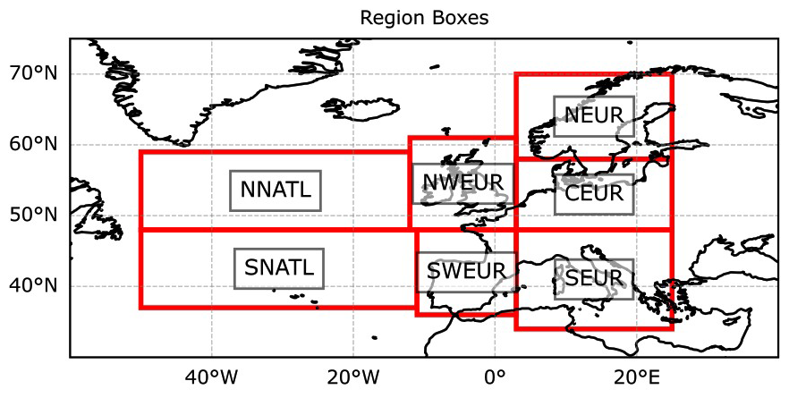
Figure A1 Regions used for regressing mean front frequency (Fig. 3) and mean frontal precipitation (Fig. 6) with resolution. Abbreviations stand for Northern North Atlantic (NNATL), Southern North Atlantic (SNATL), North-Western Europe (NWEUR), South-Western Europe (SWEUR), Northern Europe (NEUR), Central Europe (CEUR) and Southern Europe (SEUR), with the first two only being used when excluding CORDEX, because they are outside the domain.