Characteristics and dynamics of extreme winters in the Barents Sea in a changing climate

The Barents Sea is experiencing large declines in sea ice and increasing surface temperatures while at the same time it is a key region of weather variability in the Arctic. In this study, we identify extreme winter seasons in the Barents Sea, based on a multivariate method, as winters with large seasonal anomalies in one or several surface parameters encompassing surface temperature, precipitation, surface heat fluxes, and surface net radiation. The analyses are based on large-ensemble climate model data for historical (S2000) and end-of-century (S2100) projections following an RCP8.5 emission scenario. In the phase space of the considered seasonal-mean surface weather parameters, we find distinct clusters of extreme winters that are characterized by similar combinations of anomalies in these parameters. In particular, during extreme winters in S2000 simulations, anomalies in surface air temperature during extreme seasons tend to be spatially extended with their maximum amplitude over sea ice. This maximum shifts towards the continental land masses in a warmer climate (S2100), as the formation of intense warm or cold anomalies is damped by the increasing area of open ocean. Our results reveal that large anomalies in surface parameters during extreme seasons are characterized by distinct patterns of anomalous frequencies in cyclones, anticyclones, and cold air outbreaks because these weather systems are responsible for temperature and moisture advection, the formation or suppression of precipitation, and intense surface fluxes. We further show that anomalous surface boundary conditions at the beginning of a season – that is, sea ice concentration and sea surface temperatures – facilitate the formation of persistent anomalous surface conditions or further enhance atmospherically driven anomalies due to anomalous surface heat fluxes. However, a decrease in the variability of both sea ice and sea surface temperatures in S2100 indicates a decreasing importance of anomalous surface boundary conditions for the formation of future extreme winters in the Barents Sea, while the robust link shown for surface weather systems persists in a warmer climate.

1 Introduction

Global warming strongly affects the Arctic region, causing a rapid increase in surface temperatures and, at the same time, dramatic reductions in sea ice cover (e.g., Parkinson et al., 1999; Cavalieri and Parkinson, 2012; Serreze and Meier, 2019). Global climate models project continuing large changes in Arctic sea ice extent and surface conditions in the coming century (e.g., Stroeve et al., 2007; Notz and SIMIP Community, 2020), with the prospect of an ice-free Arctic during September within a few decades (Chapman and Walsh, 2007; Vavrus and Holland, 2021). Simulations show regionally and seasonally differing trends in surface variables, which are likely related to the increasing seasonality in Arctic sea ice cover and associated sea ice variability (e.g., Huang et al., 2017; Mioduszewski et al., 2019).

The region of the Barents Sea represents a hotspot of enhanced Arctic warming, commonly referred to as Arctic amplification, exhibiting some of the largest trends in surface air temperatures and sea ice extent (e.g., Parkinson et al., 1999; Cavalieri and Parkinson, 2012; Johannessen et al., 2016; Rantanen et al., 2022), which are further enhanced by an increase in oceanic heat transport by the Atlantic inflow (Årthun et al., 2012; Smedsrud et al., 2022). On top of this trend, large variations in sea ice extent, particularly in winter, result in considerable fluctuations of surface conditions such as surface air temperatures and surface heat fluxes between years, making the Barents Sea a key region of Arctic interannual variability (van der Linden et al., 2016; Dörr et al., 2021). Thereby, sea ice variability has been found to be influenced by oceanic heat transport and anomalous atmospheric circulation on interannual to multi-decadal timescales (e.g., Johannessen et al., 2016; Reusen et al., 2019; Liu et al., 2022; Siew et al., 2023), while on daily to weekly timescales, synoptic-scale weather systems are key drivers of variable surface conditions in the Barents Sea (e.g., Woods et al., 2013; Graversen and Burtu, 2016; Messori et al., 2018; Papritz, 2020; Siew et al., 2023). Extratropical cyclones link the Barents Sea to the midlatitudes and facilitate the transport of warm and moist air into the region, while cold and dry polar air is advected behind their cold fronts. Enhanced local baroclinicity along the sea ice edge further favors Arctic cyclogenesis in the Barents Sea, making it a hotspot of Arctic cyclone variability in winter (Inoue and Hori, 2011; Madonna et al., 2020; Caratsch, 2022). Although involved processes and causal relationships are a topic of debate, it has been argued that the variability of atmospheric conditions in the Barents Sea can have far-reaching effects on midlatitude weather and its extremes (e.g., Petoukhov and Semenov, 2010; Inoue et al., 2012; Jaiser et al., 2012).

Due to its large sea ice variability and high storm activity in winter, the Barents Sea is very susceptible to extreme weather events such as unusual warm air advection which can cause significant sea ice melt (e.g., Boisvert et al., 2016; Cullather et al., 2016) and rain-on-snow events (Overland, 2022), as well as intense cold air outbreaks (CAOs) from the Arctic interior, which can trigger strong air–sea heat exchanges (Fletcher et al., 2016; Papritz and Spengler, 2017). The accumulation of such events over several weeks to months can result in extreme winter seasons. Recent studies investigating extreme seasons in the Arctic region have focused mainly on seasonal Arctic temperature extremes (e.g., Cohen et al., 2010; Stroeve et al., 2011; Graham et al., 2017; Papritz, 2020). New approaches include the identification of Arctic extreme seasons based on the combination of several surface parameters as opposed to one particular variable as shown in Hartmuth et al. (2022), hereafter referred to as HA2022. There, a multivariate method is introduced using principal component analysis (PCA) to determine in an objective way the “unusualness” of a season considering seasonal anomalies in surface air temperature, precipitation, surface heat fluxes, and surface net radiation. By applying this approach to ERA5 reanalysis data, HA2022 showed that the formation of Arctic extreme seasons is highly variable and strongly determined by both atmospheric variability and surface boundary conditions, the latter particularly in regions with high sea ice variability such as the Barents Sea. On timescales of days to weeks, individual weather systems can lead to pronounced anomalies in surface variables, and the frequent occurrence of such systems can therefore contribute to the formation of extreme seasons. Additionally, anomalous surface boundary conditions can contribute to the formation of such seasons by causing comparatively weaker but more persistent anomalies throughout a season. However, a main limitation of HA2022 is the small number of extreme seasons in the ERA5 dataset. Thus, in this study, we aim to provide a statistically robust analysis of the characteristics and formation of such seasons by exploiting large-ensemble climate simulations.

The dramatic changes in surface and atmospheric conditions in the Barents Sea further suggest that future extreme winters will look differently compared to extreme winters in the present-day climate. Recent studies using climate model simulations showed that Arctic winter temperature extremes become warmer for hot extremes and less severe for cold extremes, whereby cold extremes warm faster than hot extremes (Saha et al., 2006; Kharin et al., 2013; Screen, 2014; Lo et al., 2023). This is particularly relevant in the Barents Sea, where the increasing distance to the sea ice edge is projected to contribute to a strong reduction in surface air temperature variability and cold extremes are projected to warm dramatically (Saha et al., 2006; Hartmuth et al., 2023). Further, climate models project an increase in frequency and intensity of both winter warm events and precipitation extremes (Saha et al., 2006; Kharin et al., 2013; Graham et al., 2017; Bogerd et al., 2020). Due to the increase in mean temperature, the rainfall ratio will increase strongly in future precipitation, which additionally enhances the probability of severe conditions such as rain-on-snow events (Bintanja et al., 2020; McCrystall et al., 2021).

Many questions remain with regard to the formation and characteristics of extreme winters in the Barents Sea, in particular in a warming climate. For one thing, the relative importance of changes in the seasonal mean vs. interannual variability of surface parameters is still under debate (Overland, 2022; Lo et al., 2023). Further, the question arises if future extremes are driven by similar dynamic and thermodynamic processes as present-day extremes, as well as how the drastic change in surface conditions will affect their characteristics. A detailed and systematic analysis of extreme winters in the Barents Sea, as performed in this study, can lead to new insights regarding the processes leading to such seasons and their relation to the general atmospheric circulation.

The goal of this paper is to complement the results in HA2022 with a detailed analysis of the characteristics and dynamics of extreme winters in the Barents Sea in both CESM1 (Community Earth System Model version 1) present-day (S2000) and end-of-century (S2100) simulations. Thereby, using over 1000 years of large-ensemble climate model data per time period allows for a robust statistical investigation of extreme winters and the evaluation of future projections. The aim is to address the following research questions:

1. In a warmer climate, is there a change in the relative importance of selected surface parameters for the interannual variability of winters in the Barents Sea?

2. What are the characteristics of extreme winters in the Barents Sea and are they related to the unusual occurrence of synoptic-scale weather systems and anomalous boundary conditions?

3. To what extent do the characteristics of extreme seasons in the Barents Sea change in a warmer climate?

This study is organized as follows. The data and methods used are presented in Sect. 2. Results of the PCA are discussed in Sect. 3 with particular emphasis on climate change effects. Subsequently, we analyze the characteristics of clusters of extreme winters in the Barents Sea and the role of synoptic-scale weather systems for the formation of anomalous surface conditions on the seasonal timescale. Results for S2000 simulations are presented in Sect. 4 and for S2100 in Sect. 5, before we conclude our results in Sect. 6.

2 Data and method

2.1 CESM1 data

In this study, we assess simulations with the fully-coupled Community Earth System Model version 1 (CESM1; Hurrell et al., 2013), which are initialized by using restart files from the CESM large ensemble project (CESM-LE; Kay et al., 2015). In addition to the original CESM-LE data consisting of 35 ensemble members, based on the first and second members of that dataset, further simulations are initialized following small perturbations of the initial atmospheric temperature field (for further details, see Röthlisberger et al., 2020). In total this results in a 105-member ensemble for a historical period (S2000; 1990–2000, 1155 winter seasons) and an end-of-century period (S2100; 2091–2100, 1050 winter seasons). For S2100, simulations are run under a Representative Concentration Pathway 8.5 (RCP8.5) forcing scenario. At a spatial resolution of approximately 1°, we use seasonal-mean surface-level fields of 2 m temperature (T), precipitation (P; sum of rain and snow), surface sensible (H_S) and latent (H_L) heat fluxes, surface net shortwave (R_S) and longwave (R_L) radiation, sea surface temperature (SST), and sea ice concentration (SIC). In addition, the sum of surface heat fluxes and surface net radiation ($H_{\mathrm{S}}+H_{\mathrm{L}}+R_{\mathrm{S}}+R_{\mathrm{L}}$) is defined as the surface energy budget and denoted by E_S. Thereby, positive values of E_S denote a net energy flux into the ocean, while negative E_S values indicate a net energy flux into the atmosphere. SST is only defined at grid points over the ocean where SIC ≤ 50 %.

Our analyses in this study are based on seasonal anomalies relative to a climatology. Therefore, a time-mean climatology is calculated at each grid point as temporal mean over all simulated seasons, and seasonal anomalies are defined as deviation of seasonal-mean values from this climatology. To account for the transient radiative forcing including the 1991 Pinatubo eruption in all S2000 members, we remove this forced signal from the S2000 ensemble mean, yielding a transient climatology (see Fig. 2.7 in Hartmuth et al., 2023). This way, we avoid a bias in the seasonal anomalies and subsequent bias in the occurrence of extreme seasons. Throughout this study, we denote seasonal anomalies of a variable χ with respect to the transient climatology as χ^*.

For this study, we focus on the winter season (December–February, DJF). Our analyses are performed for the region of the Barents Sea that is already mostly ice free in S2000. Therefore, we choose the climatological sea ice edge as the boundary of this area. To this end, we apply a threshold for the ensemble mean winter sea ice concentration in S2000 (SIC_S2000) of 50 % and define the area of the Barents Sea where SIC_S2000 < 50 % as our region of interest, referred to as BS. Applying this method, we focus on the southern, western, and central parts of the Barents Sea, which is usually defined as the area enclosed between Svalbard, Franz Josef Land, Novaya Zemlya, and the northern coast of Scandinavia (International Hydrographic Organization, 1953). Note that irrespective of the changing sea ice coverage, the same region is used for the analysis of S2100 simulations. When analyzing spatiotemporal averages of the surface parameters, we first take the seasonal mean before calculating a spatial average over the BS region.

To investigate synoptic features such as cyclones and anticyclones, we apply weather system identification schemes as described in Sprenger et al. (2017). Based on 6 h sea level pressure (SLP) data, cyclones and anticyclones are defined as objects that cover the area around a SLP minimum and maximum, respectively, and are thereby delimited by the outermost closed SLP contour. We further define marine CAOs at grid points over the ocean where SIC ≤ 50 %, at times when the 900 hPa sea–air potential temperature difference (θ_SST−θ₉₀₀) is larger than ≥ + 4 K (Papritz and Spengler, 2017). Each weather system is identified as an object described by a two-dimensional binary field with a value of 1 at grid points inside the object and 0 outside. By time-averaging these binary fields, we calculate fields of mean cyclone frequency (f_c), anticyclone frequency (f_a), and CAO frequency (f_CAO). For example, f_c = 0.3 at a given grid point indicates that at 30 % of all times, a cyclone is present at that grid point. Spatiotemporal averaging over the BS region yields daily or seasonal-mean cyclone frequencies for this area. Similarly, the winter-mean weather system frequency anomaly is calculated as the deviation of the spatially averaged winter-mean weather system frequency from the climatology. We further consider relative frequency anomalies, which for a specific weather system are calculated (in %) as

$$\begin{array}{}\text{(1)}& {\displaystyle \frac{f_{\text{seas}}-f_{\text{clim}}}{f_{\text{clim}}}}\times \mathrm{100},\end{array}$$

where f_seas and f_clim denote the spatially averaged winter-mean weather system frequencies for the season and the climatology, respectively.

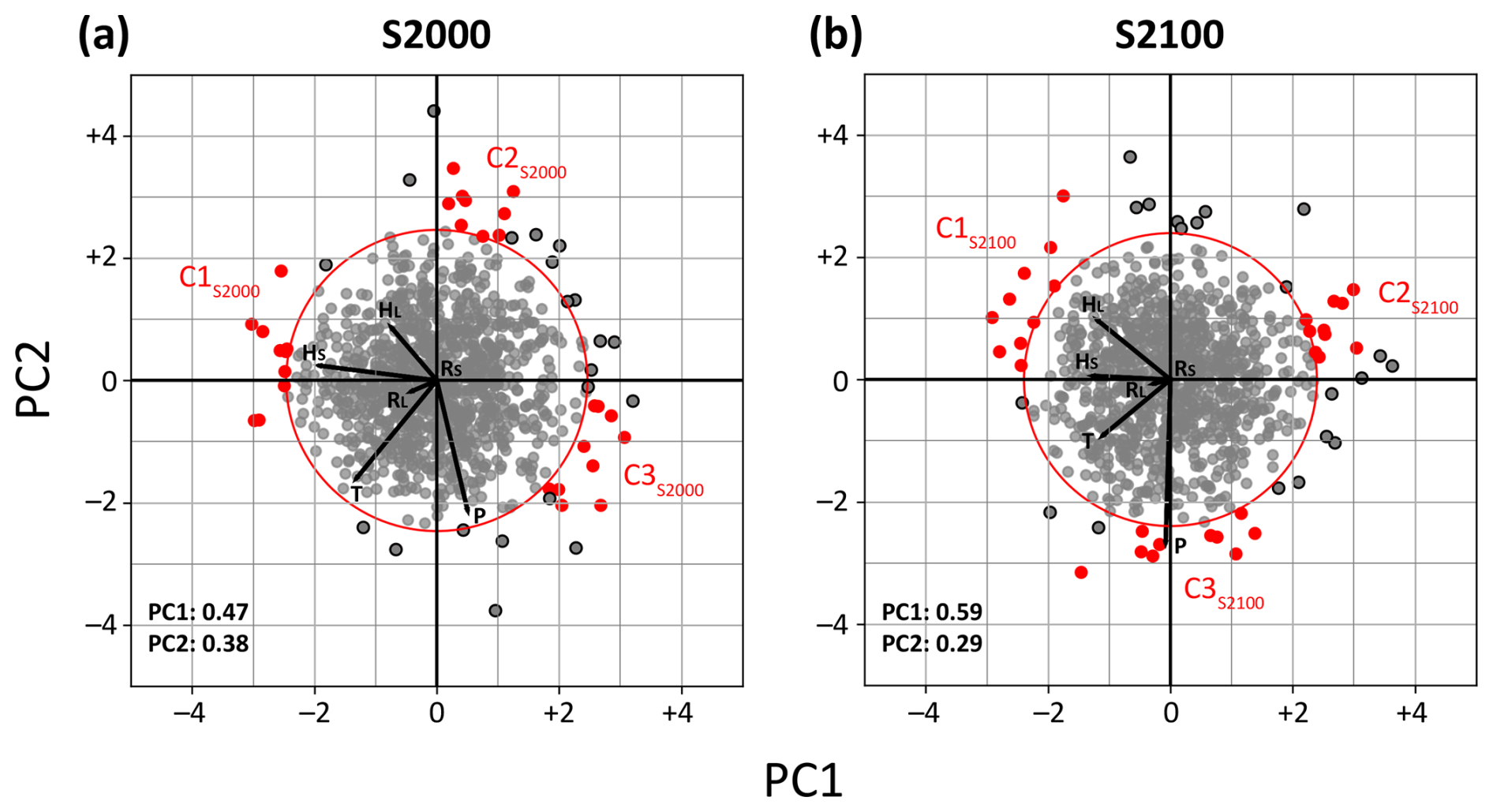
Figure 1 PCA biplot for BS in (a) S2000 and (b) S2100 with PC1 and PC2 along the x axis and y axis, respectively. Normal seasons are represented by grey dots, extreme seasons are those outside the red circle, which represents the 50th largest d_M value. Three clusters of extreme seasons in each period are indicated by red dots. Black lines represent the coefficients of the precursor variables. The variance values explained by PC1 and PC2, respectively, is given in the lower left corner of each panel.

2.2 Definition of extreme seasons

Extreme winters in BS are identified using the PCA-based method first introduced in HA2022. The PCA allows us to reduce the dimensionality of a six-dimensional phase space, spanned by the spatially averaged seasonal anomalies of T, P, H_S, H_L, R_S, and R_L, to two dimensions. Note that in this study PCA is applied in P mode as opposed to S mode (following Fig. 9 in Richman, 1986), which is commonly used in climate studies. The resulting first and second principal components (PC1 and PC2) maximize the explained proportion of the total inter-seasonal variability of the six-dimensional precursor phase space. Due to the combination of several parameters, the interplay between these variables, which refers to the correlations between the different variables, is taken into account. This makes the method applicable to different seasons and allows for a comparison of extreme seasons considering the heterogeneity of the Arctic surface. In addition, the multivariate approach enables the investigation of a broader spectrum of extreme seasons, as also seasons that are extreme only due to the unusual combination of anomalies in several surface parameters are taken into account.

The result of the PCA can be illustrated using a biplot as shown in Fig. 1. Each dot represents one winter season in BS, and the distance of a season to the origin of the PC1−PC2 phase space, the so-called “Mahalanobis distance” (d_M), is a measure for the unusualness of the season (for more details, see Sect. 2 in HA2022). Here, the 50 winters with the largest d_M are defined as extreme winters (dots outside the red circle in Fig. 1), which corresponds to a return period of approximately 20 years.

The closer two winters are in the biplot, the more similar their seasonal anomalies are in the six surface parameters. Radial vectors show the relative contribution of the precursor variables to PC1 and PC2, where relatively shorter (longer) vectors indicate a smaller (larger) contribution of the precursor to the explained variance. The relative position of two vectors indicates the correlation between both corresponding precursors, with uncorrelated precursors resulting in approximately perpendicular vectors and more strongly correlated precursors resulting in more parallel vectors. The representation of this correlation in a PCA biplot is, however, more precise when the variance explained by PC1 and PC2 is higher (Gabriel, 1971, 1972). The relative position of a season with respect to the precursor vectors refers to the contribution of the different surface variables to the d_M value of this season. For example, colored seasons at the top of the biplot shown in Fig. 1a are characterized by negative seasonal anomalies in T and P, while colored seasons to the left show positive seasonal anomalies in H_S.

2.3 Identification of extreme season clusters

In order to statistically evaluate extreme winters in BS in current and future climate states, we define clusters of extreme seasons in the respective PCA biplot. Thereby, we aim to contrast collections of similar seasons (i.e., closely spaced in the PCA biplot), whereby the distinct clusters differ strongly in their characteristics (i.e., located in different directions of the PCA biplot). For example, in the S2000 PCA biplot (Fig. 1a), we can already identify several distinct clusters by eye. However, we use the following objective approach to identify clusters of 10 seasons, which allow for a meaningful statistical comparison between different clusters. First, we consider only the azimuthal position of the extreme seasons in the biplot, and we determine for each group of 10 adjacent extreme seasons the angle segment in the biplot that encloses this group. In a second step, the three non-overlapping groups with the smallest angle segment are chosen for the cluster analysis in Sects. 4 and 5. They are indicated by red dots in Fig. 1. Due to the distribution of extreme seasons in the PCA biplot for S2100 (Fig. 1b), some compact collections of extreme seasons such as a group of very dry seasons at the top of the biplot are disregarded, as they do contain fewer than 10 seasons, hampering a statistical analysis.

3 Interannual variability of surface parameters in present-day and future climates

3.1 S2000

Here we present the results of the PCA of CESM1 simulations in S2000 for the BS region (Fig. 1a) and discuss them against the background of the results shown for a similar region in the ERA5 dataset in HA2022. This is an important step to validate the representation of the variability of surface variables in CESM1, which is a requirement for a meaningful interpretation of climate change effects. For S2000, a slightly lower explained variance by the first two principal components, PC1 and PC2, in CESM1 (84.5 %) implies that the original six-dimensional precursor phase space is slightly less well represented by the first two PCs compared to ERA5 (95 %). Winter annual variability in CESM1 is almost in equal parts determined by T, P, and the surface heat fluxes, whereas P contributes by far the most to interannual variability in the ERA5 dataset (see Fig. 7c in Hartmuth et al., 2022). Note, however, that due to the remoteness of the study area the accuracy of ERA5 precipitation fields is potentially limited.

Values of the combined magnitude of the seasonal anomalies of the precursor variables in the two-dimensional PCA phase space, which we denote by d_M (see also Sect. 2.2), are within a similar range for both datasets. As the number of available seasons is much larger in CESM1 compared to ERA5, it is expected that seasons with larger anomalies can be found in CESM1, particularly as both datasets exhibit a similar variability for most of the precursor variables (see chapter 2 in Hartmuth, 2023a).

While in HA2022 extreme seasons in the ERA5 dataset are defined based on a fixed d_M threshold (d_M≥3), here we choose the 50 seasons exhibiting the largest d_M value as extreme seasons in CESM1 (see Sect. 2.2), which corresponds to a threshold of d_M = 2.47 for S2000 simulations. Extreme seasons, shown as dots outside the red contour in Fig. 1, form clusters at distinct locations in the biplot. Seasons within a cluster exhibit a similar combination of seasonal anomalies such as, for instance, several extreme winters in S2000 that are grouped at the top of the biplot (Fig. 1a). As they are located in the opposite direction of the T and P precursor vectors, we can assume that these seasons show negative seasonal anomalies in both T and P and are, thus, particularly cold and dry. We will further analyze the large-scale anomalies in surface parameters and weather systems linked to this group of extreme winters in Sect. 4.

3.2 S2100

We now compare results of the PCA in S2100 simulations (Fig. 1b) to the results for S2000 discussed beforehand. In S2100, PC1 and PC2 explain 87.6 % of the total variance for winters in BS, which is a similar value compared to S2000. The threshold for extreme winters in S2100 is d_M = 2.40, which implies that there is no notable increase or decrease in the normalized amplitude of combined seasonal anomalies of future extreme winters.

Small changes in the representation of the surface variables in the PCA phase space reflect that interannual variability in winter conditions in the Barents Sea will be governed similarly by T, P, and the surface heat fluxes in a warmer climate with a slightly increasing contribution of P compared to the other surface variables. As the region is already largely ice free in the present-day climate, changes in sea ice variability are comparatively small; therefore, the correlation between the variables remains largely unchanged (see Supplement Tables S1 and S2 for correlation values between precursor variables and their change between S2000 and S2100, respectively).

In the following, we will focus on clusters of extreme winters in BS to investigate the characteristics and formation of such seasons in both S2000 and S2100 simulations. However, due to the different reference climate states used in the respective PCAs, the distribution of selected extreme season clusters in the PCA biplot, and the slightly different combination of precursor contributions, the clusters between both periods are not directly comparable. Therefore, we will analyze both S2000 and S2100 clusters separately, and while this evaluation serves less as a direct comparison of extreme seasons in present-day and future conditions, we will discuss some general differences between both climate states in Sect. 6.

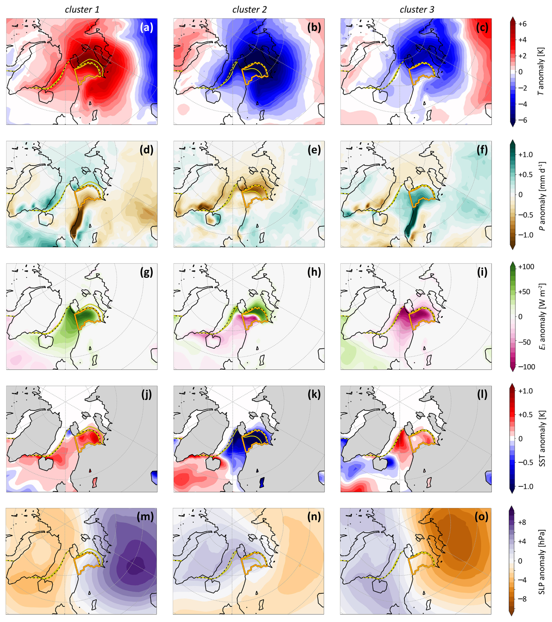
Figure 2 Seasonal anomalies of (a–c) T (T^*, in K), (d–f) P (P^*, in mm d⁻¹), (g–i) E_S (${E_{\mathrm{S}}}^{*}$, in W m⁻²), (j–l) SST (SST^*, in K), and (m–o) SLP (SLP^*, in hPa) for extreme winters in cluster 1 (left column), cluster 2 (middle column), and cluster 3 (right column) in S2000. The solid yellow line shows the mean sea ice edge for the respective cluster, and the dashed yellow–black line shows the climatological sea ice edge. The BS region is shown by the orange contour.

4 Extreme winters in S2000

4.1 Seasonal anomalies of surface parameters

While the position of clusters of extreme winters in the PCA biplot already gives an idea about the surface parameters that are particularly anomalous in these winters, there is no information from the biplot about the spatial distribution and actual magnitude of these anomalies. Figure 2 shows spatial composites of the seasonal anomalies of T (denoted as T^*), P (P^*), E_S (${E_{\mathrm{S}}}^{*}$), and SST (SST^*) for each cluster in S2000.

Winters in cluster 1 (C1_S2000 in Fig. 1a) are characterized by positive anomalies in surface heat fluxes (particularly H_S) and a positive T^*. Figure 2a shows an extensive area with positive T^* covering large parts of the Arctic Ocean that is particularly pronounced along the Scandinavian and Russian coastline and over the sea-ice-covered part of the Barents Sea, where it coincides with a reduction in SIC (yellow lines in Fig. 2a). At the same time, a positive ${E_{\mathrm{S}}}^{*}$ (i.e., net energy flux into the surface) is particularly pronounced over the open ocean (Fig. 2g) and spreads far into the Norwegian Sea. The shift of the sea ice edge to the north coincides with a consistently positive seasonal anomaly in SSTs (Fig. 2j). A small negative P^* is shown in BS, which is more evident along the Norwegian coast (Fig. 2d). Furthermore, these winters feature a dipole in SLP^* with a pronounced positive SLP^* over the European continent (Fig. 2m).

Winters in cluster 2 (C2_S2000 in Fig. 1a) are located opposite to the T and P vectors in the PCA biplot, which implies that these winters are unusually cold and dry. Figure 2b shows indeed a spatially extended negative T^*, which is most strongly pronounced in the eastern Barents Sea where the sea ice extends anomalously far south. Interestingly, the spatial extension of this negative T^* is very similar to that of the positive T^* shown for cluster 1 with its maximum over the sea-ice-covered part of the Barents Sea. The area within BS that experiences anomalous sea ice cover exhibits a pronounced negative P^* (Fig. 2e). In terms of E_S, the winter seasons of this cluster exhibit a dipole with a positive ${E_{\mathrm{S}}}^{*}$ where more sea ice than usual is present and a negative ${E_{\mathrm{S}}}^{*}$ over the open ocean (Fig. 2h). While the increased ice cover reduces air–sea interactions in the northeastern part of BS, the southward shift of the sea ice edge likely causes anomalous oceanic heat loss over the southwestern part of BS, an area which is climatologically further away from the sea ice edge. The anomalous sea ice cover of this cluster further coincides with a pronounced negative anomaly in SSTs, which extends into the Norwegian Sea (Fig. 2k). Winters in cluster 2 exhibit a reversed dipole in SLP^* anomalies compared to cluster 1, although with a weaker amplitude (Fig. 2n).

Winters in cluster 3 (C3_S2000 in Fig. 1a) are located opposite to winters in cluster 1 in the PCA biplot and, thus, include seasons that are characterized by large negative seasonal anomalies in surface heat fluxes. This is illustrated in Fig. 2i, which shows a pronounced negative ${E_{\mathrm{S}}}^{*}$ in the whole BS region and in particular over the open ocean, where it further coincides with a positive P^* (Fig. 2f). While T^* takes consistently negative values across the region, the center of this negative anomaly is located over the ice-covered part of the eastern Barents Sea and the Kara Sea (Fig. 2c). It is noteworthy that despite the negative T^*, a slightly positive anomaly in seasonal-mean SSTs is shown in the BS region and even more pronounced in the Nordic Seas (Fig. 2l). The sea ice edge in these winters is close to climatology, and a pronounced negative SLP^* is shown in the region of the Ural Mountains (Fig. 2o).

A detailed analysis of the daily variability in anomalies of surface parameters which we refer to as “substructure” of an extreme season (Röthlisberger et al., 2021; Hartmuth et al., 2022) is presented in the Supplement. Based on several case studies (see time series in Supplement Figs. S1 and S2), we show that recurrent short-term events linked to the occurrence of weather systems facilitate the formation of seasonal anomalies in surface atmospheric conditions. However, we are not yet able to fully understand the large-scale processes as well as the interplay between weather systems and surface boundary conditions that lead to the formation of extreme winters in BS. Thus, in the following we analyze the spatial distributions of anomalies in the occurrence of cyclones, anticyclones, and CAOs, which will improve our understanding of how weather systems affect the evolution of persistent anomalous surface conditions in BS.

4.2 Seasonal anomalies in weather system frequencies

To investigate the large-scale dynamics associated with extreme seasons in BS, we analyze anomalies in the occurrence of weather systems that affect this region. For this analysis, we slightly increase the size of the BS region to account for the influence of weather systems also if they are not directly colocated with the BS region. In a first step, we examine for each 6 h time step during each winter whether the mask of a weather system object (see Sect. 2.1) overlaps with the enlarged BS region. If this is the case, we consider this mask for the calculation of the seasonal weather system frequency anomaly. Note that a frequency anomaly for a specific cluster is calculated as the deviation from a climatology. This climatology is obtained as the mean over all masks that overlap with the enlarged BS region in all simulations. As the distribution of this climatology is not necessarily symmetric with respect to the BS region and as the number of values contributing to the climatology per grid point decreases with increasing distance to BS, potential biases due to the design of this method will be considered.

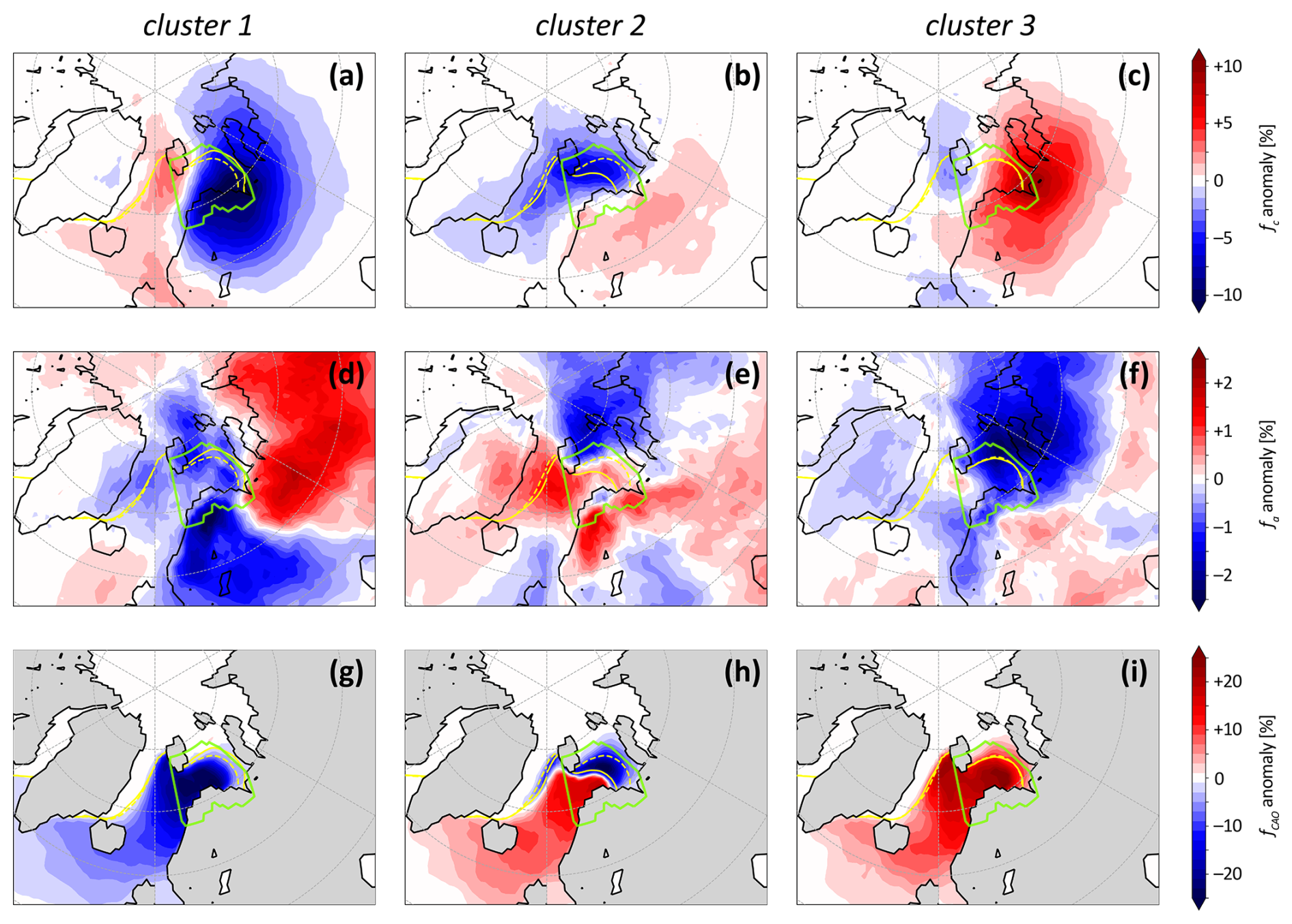
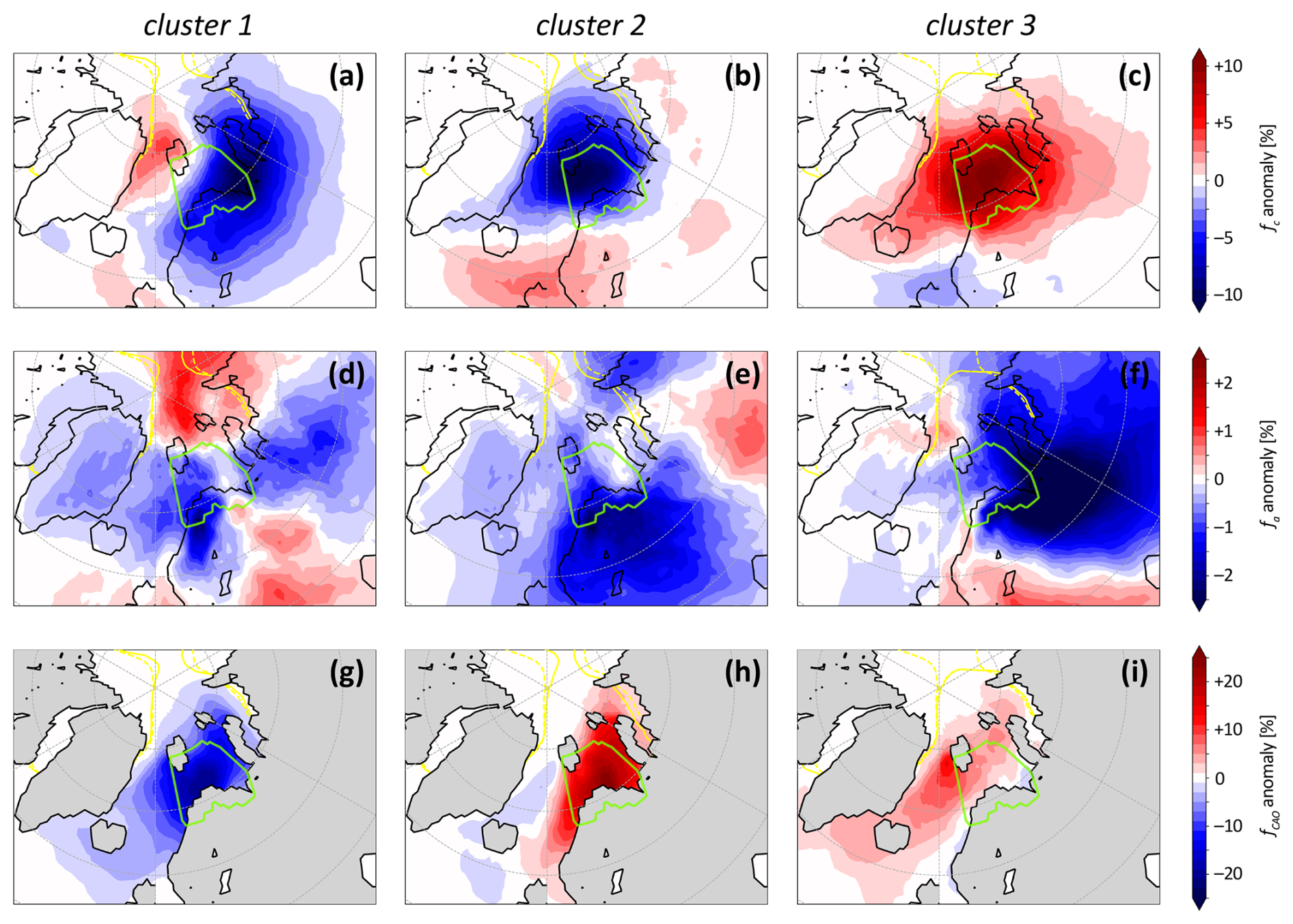
Figure 3 Absolute seasonal anomalies in (a–c) cyclone frequency (${f_{\mathrm{c}}}^{*}$, in %), (d–f) anticyclone frequency (${f_{\mathrm{a}}}^{*}$, in %), and (g–i) CAO frequency (${f_{\mathrm{CAO}}}^{*}$, in %) for extreme winters in (a, d, g) cluster 1, (b, e, h) cluster 2, and (c, f, i) cluster 3 as described in Sect. 2.3. The solid yellow line depicts the mean sea ice edge for the respective cluster and the dashed yellow line the climatological sea ice edge in S2000 (SIC_clim = 0.5). The enlarged BS region is shown by the green contour.

We have shown that winters in cluster 1 are mainly characterized by positive anomalies in T and E_S and a concurrent lack of sea ice. As can be seen from Fig. 3a, a more meridional propagation of cyclones results in a slight surplus of cyclones in the Nordic Seas and the northwestern part of BS and a simultaneous lack of cyclones extending from Scandinavia to the Kara Sea which is, however, more pronounced compared to the positive ${f_{\mathrm{c}}}^{*}$. This is consistent with the results in Hartmuth et al. (2023), who showed a dipole in ${f_{\mathrm{c}}}^{*}$ for extremely warm winters in this area and at the same time a local negative ${f_{\mathrm{c}}}^{*}$ during extremely dry seasons. The composite shown in Fig. 3a can be regarded as a combination of these two patterns due to the positive T^* and negative P^* featured by winters in cluster 1. Given this pattern, it is plausible that during these winters the advection of cold and dry air in the cold sectors of cyclones is strongly reduced and that most of the time only the warm sector of a cyclone is located in the BS region, causing a net increase in T. This could further explain the pronounced lack of CAOs (Fig. 3g) despite a positive SST^* in BS (Fig. 2j), which additionally enhances the formation of a positive T^*. Next to a reduced f_c and f_CAO, winters in cluster 1 also show a weakly negative ${f_{\mathrm{a}}}^{*}$ (Fig. 3d) in BS. Thereby, a pronounced dipole in ${f_{\mathrm{a}}}^{*}$ is shown over the continent with a relative lack of anticyclones over Scandinavia and a surplus of anticyclones over Russia which further favors the advection of comparatively warm air from the continent (see Fig. 2a).

In contrast to the warm winters in cluster 1, cluster 2 comprises of particularly cold and dry winters, which presumably experience a surface preconditioning in the form of a positive SIC anomaly that already exists at the beginning of a winter (see Fig. S1c, d). Figure 3b shows a negative ${f_{\mathrm{c}}}^{*}$ for most of BS and in particular for the area with increased SIC, while slightly more cyclones than usual are found over Scandinavia. This pattern is in line with the results found for cold and dry winters in this area in Hartmuth et al. (2023). As cyclones tend to pass to the south of BS rather than directly across the region, the transport of relatively warm and wet air is confined to these areas, while BS is more strongly affected by the advection of cold and dry air in the wake of these cyclones. At the same time, this pattern favors the advection of air from the cold air reservoir over the continent (see Fig. 2b). This cluster further features a dipole with a positive ${f_{\mathrm{a}}}^{*}$ over Scandinavia and the Nordic Seas and vice versa a negative ${f_{\mathrm{a}}}^{*}$ towards the north of BS (Fig. 3e). This pattern further favors the advection of relatively cold and dry air from the high Arctic towards the open ocean. The combination of an enhanced advection of cold and dry air from the regions with exceptionally cold air over the sea ice and the continent as well as a shifted sea ice edge results in a positive ${f_{\mathrm{CAO}}}^{*}$ over the open ocean in BS (Fig. 3h). Simultaneously, a concurrent reduction in CAOs is found in the area of extended sea ice cover.

Winters of cluster 3 exhibit recurrent events of strong oceanic heat loss resulting in an overall negative seasonal ${E_{\mathrm{S}}}^{*}$, which can be linked to the frequent occurrence of CAOs (see Fig. S1e, f). Figure 3i shows a pronounced positive ${f_{\mathrm{CAO}}}^{*}$ over BS and the Nordic Seas. As no significant anomaly in SIC can be found for these winters, an eastward shift in the occurrence of cyclones as shown in Fig. 3c is most likely causing this positive anomaly in ${f_{\mathrm{CAO}}}^{*}$. The increased occurrence of cyclones towards the east of BS favors the advection of cold and dry air from the ice-covered northern part of the Barents Sea (see T anomaly in Fig. 2c) and the Kara Sea, which then results in enhanced surface heat fluxes into the atmosphere. At the same time, this pronounced positive ${f_{\mathrm{c}}}^{*}$ facilitates the overall positive P^* of seasons in this cluster. The relative absence of anticyclones over the eastern Barents Sea, the Kara Sea, and along the Siberian coast (Fig. 3f) indicates that the negative T^* in this region is mainly driven by the shift in cyclone-related advection of cold and dry air as opposed to radiative cooling within persistent anticyclones.

When comparing anomalies in weather system frequencies for the different clusters, it becomes apparent that each cluster is characterized by distinct patterns of such anomalies, which can be related to typical patterns associated with exceptionally large seasonal anomalies in T and P (Hartmuth et al., 2023). In addition, distinct anomalies in f_CAO are found for each cluster and can be linked to both the anomalous frequencies and pathways of cyclones, which affect the advection of cold and dry air from the Arctic interior and Eurasian continent towards BS, and shifts in the sea ice edge. This combination of anomalous circulation patterns and anomalous surface boundary conditions can cause the formation of a strong dipole in ${f_{\mathrm{CAO}}}^{*}$ such as for cluster 2, which further results in a dipole of surface heat flux anomalies (see Fig. 2h) but only a small spatially averaged anomaly. In contrast, for winters in cluster 3, which show on-average sea ice extent, the anomalies in f_CAO are mainly caused by anomalies in the atmospheric circulation and cause an overall increase in surface heat fluxes, resulting in a distinct positive ${E_{\mathrm{S}}}^{*}$. Note that the spatial extension of the CAO anomalies towards lower latitudes is partially affected by the design of the method (see Sect. 2.3) as large coherent masks of CAOs can result if distinct CAO events in the BS region and along the Greenland coast occur at the same time.

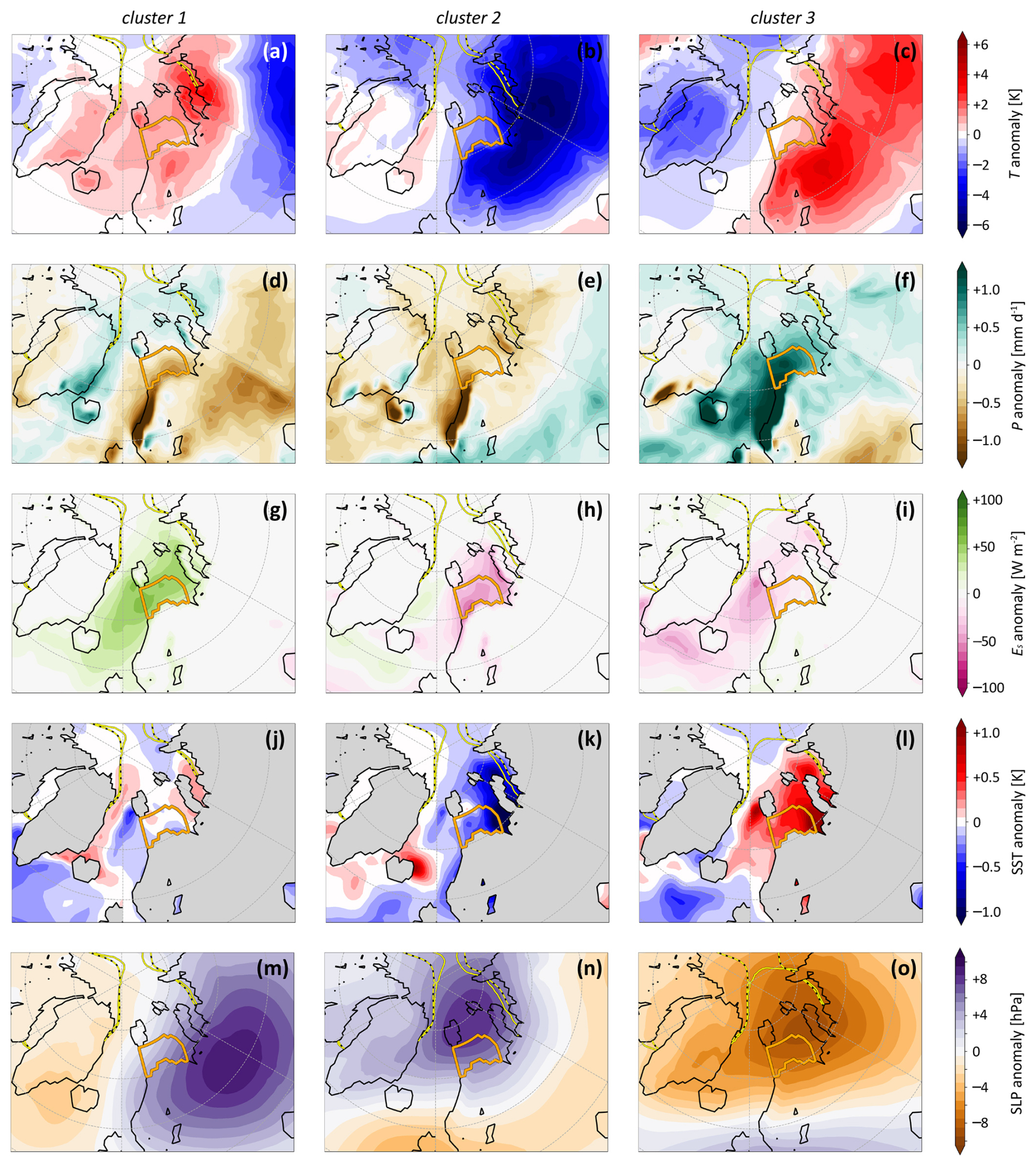
Figure 4 Same as Fig. 2 but for extreme winter clusters in S2100.

5 Extreme winters in S2100

5.1 Seasonal anomalies of surface parameters

After evaluating the processes leading to the formation of extreme winters in BS in the present-day climate, we now repeat this analysis for future winters in BS. In the following section, we again compare three different clusters of extreme winter seasons based on the PCA biplot for S2100 (see Fig. 1b). As mentioned beforehand, due to the design of our method we cannot provide a direct comparison of the same type of extreme winters in both S2000 and S2100. Instead, this analysis aims to shed light on the question of how future extreme winters in BS are characterized and whether the relative importance of weather systems vs. surface boundary conditions for the formation of future extreme winters in BS is expected to change.

Extreme winters in cluster 1 (C1_S2100 in Fig. 1b) feature positive seasonal anomalies in the surface heat fluxes and in particular in H_L (Fig. 1b). Figure 4g shows that a pronounced positive ${E_{\mathrm{S}}}^{*}$ in BS extends into the Kara Sea and Nordic Seas for these winters. This anomaly coincides with a slightly positive T^*, which is, however, more pronounced in the region of the Kara Sea (Fig. 4a). At the same time, a negative P^* occurs, in particular in the southern part of BS, close to the Norwegian coast (Fig. 4d). In terms of SSTs, winters in cluster 1 show no particularly pronounced anomalies (Fig. 4j). A positive SLP^* is shown over the European continent as opposed to a smaller negative SLP^* to the southeast of Greenland (Fig. 4m).

Cluster 2 (C2_S2100 in Fig. 1b) includes several unusually cold winter seasons, as can be concluded from their position opposite to the T precursor vector in the PCA biplot (see Fig. 1b). Analyzing the spatial distribution of this negative T^* shows that it is most pronounced over the continental land masses of Scandinavia and Russia, while the BS region is only located at the edge of this anomaly (Fig. 4b). The cold surface air temperature correlates with SSTs being below climatology in both the Barents Sea and Kara Sea (Fig. 4k). Further, winters in this cluster feature spatially coherent weakly negative anomalies in both P and E_S (Fig. 4e, h) as well as a distinct positive SLP^* to the north of BS (Fig. 4n).

Winters in cluster 3 (C3_S2100 in Fig. 1b) feature particularly wet seasons. Figure 4f shows that the positive P^* is especially pronounced along the Norwegian coast and in the western part of BS. While these winters show on average only a small positive T^* in BS, a much larger positive T^* occurs over Scandinavia and Russia (Fig. 4c). This anomaly is possibly linked to a positive anomaly in SSTs, which is particularly pronounced close to the coast and extends into the Nordic Seas, Barents Sea, and Kara Sea (Fig. 4l), a region characterized by a negative SLP^* in these winters (Fig. 4o). In terms of E_S, winters in cluster 3 feature on average only a weakly positive anomaly (Fig. 4i).

With regard to their substructure, we find that the absence of sea ice in S2100 is associated with a reduced daily variability in both T and E_S, which becomes visible in the reduced standard deviation of both variables (see Figs. S1 and S2). In general, smaller daily-mean anomalies are found for all parameters except P in S2100 compared to anomalies in S2000. However, the anomalies are still comparable relative to the respective climatology, owing to the reduced variability in many surface parameters in BS in a warmer climate.

Figure 5 Same as Fig. 3 but for extreme winter clusters in S2100 shown in Fig. 1b.

5.2 Seasonal anomalies in weather system frequencies

We now assess the dynamics of extreme winters in S2100 by evaluating anomalies in f_c, f_a, and f_CAO, which, again, show pronounced patterns for the distinct clusters. Extremely warm winters in cluster 1 are characterized by a particular lack of cyclones along the Scandinavian coastline and in the eastern Barents Sea as well as a small positive ${f_{\mathrm{c}}}^{*}$ along the Fram Strait (Fig. 5a), a pattern which we have also seen for similar seasons in cluster 1 in S2000 (Fig. 3a). While this pattern favors the advection of relatively warmer air from the North Atlantic, we assume that a large part of the positive T^* in BS results from the absence of cold air advection into this area. This is supported by the strong negative ${f_{\mathrm{CAO}}}^{*}$ during these winters (Fig. 5g), which is likely linked to the lack of cyclones advecting cold and dry air in their cold sector, facilitating the formation of both a positive T^* and ${E_{\mathrm{S}}}^{*}$ (see Fig. 4a, g). In addition, we find a dipole in ${f_{\mathrm{a}}}^{*}$ with increased anticyclone activity over the Arctic Ocean and a relative lack of anticyclones in a latitudinal band around BS (Fig. 5d).

The cold and dry winters in cluster 2 experience a general lack in both cyclones and anticyclones in BS as cyclones seem to move more zonally to the south of the region (Fig. 5b, e). Thus, these cyclones advect warm and moist air further south, while facilitating the transport of cold and dry continental air (Fig. 4b) into the BS region. This matches the positive ${f_{\mathrm{CAO}}}^{*}$ (Fig. 5h), which further favors the persistence of cold and dry conditions. Interestingly, although two winters from this cluster show a positive ${f_{\mathrm{a}}}^{*}$ (Fig. S2c, d), which might further facilitate the formation and/or persistence of cold and dry air at the surface due to enhanced radiative cooling, on average the winters of cluster 2 show a weakly negative ${f_{\mathrm{a}}}^{*}$ in BS (Fig. 5e). This indicates that the strongly negative T^* and P^* of these winters are mainly caused by an increase in the frequency of CAO events associated with a shift in cyclone occurrence as opposed to enhanced radiative cooling in surface anticyclones.

A local surplus in cyclones and simultaneous lack of anticyclones is characteristic for wet winters in both present-day and future simulations (Hartmuth et al., 2023). Here, we also show this characteristic for extremely wet winters in cluster 3 (Fig. 5c, f). A positive ${f_{\mathrm{CAO}}}^{*}$ with its maximum over the Nordic Seas reflects the enhanced cold air advection associated with the surplus of cyclones passing through BS in these winters (Fig. 5i).

To summarize, similar to the analyses of S2000 simulations, S2100 extreme winters in BS show pronounced anomalies in the occurrence of synoptic weather systems. In particular, the similar importance of a locally enhanced occurrence of cyclones for extremely wet winters and a decreased occurrence for dry winters in both climate states is in line with our findings in Hartmuth et al. (2023), where we concluded that the large-scale patterns determining seasonal T and P extremes are largely unaffected by global warming. However, due to the increasing distance of the region to the sea ice edge in a warmer climate, f_CAO anomalies are mainly associated with anomalies in f_c and, thus, with anomalies in the atmospheric circulation, and not primarily associated with anomalies in sea ice extent, which reflect anomalous surface boundary conditions.

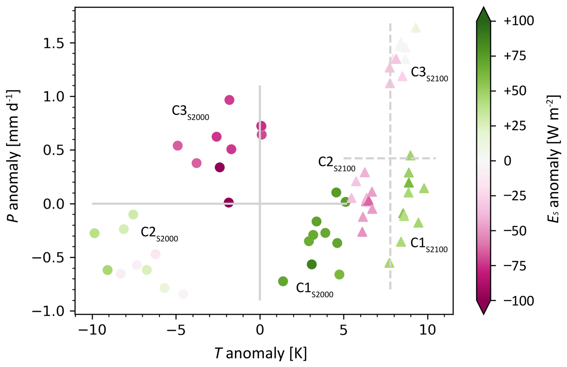
Figure 6 Seasonal anomalies with respect to S2000 of T (in K) along the x axis and P (in mm d⁻¹) along the y axis for extreme winter clusters in S2000 (dots) and S2100 (triangles). Grey lines show climatological mean T and P values in this relative phase space for S2000 (solid) and S2100 (dashed). Markers are colored by seasonal anomalies of E_S (in W m⁻²). Note that for E_S shown anomalies are relative to the respective climatology.

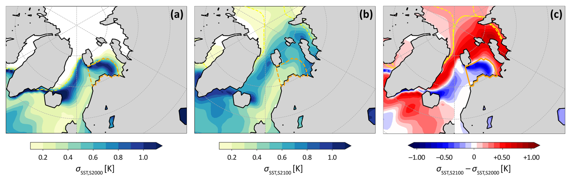
Figure 7 SST standard deviation (in K) in (a) S2000 (σ_SST,S2000) and (b) S2100 (σ_SST,S2100). Panel (c) shows the difference between S2000 and S2100 (σ_SST,S2100−σ_SST,S2000). The climatological sea ice edge is shown as a solid yellow line for S2000 and as a dashed yellow line for S2100. The BS region is marked with the orange line.

6 Discussion and conclusions

In this study, we investigate the characteristics and dynamics of extreme winters in the Barents Sea in a changing climate. Our results extend the analysis of present-day Arctic variability and extreme seasons in the ERA5 reanalysis in Hartmuth et al. (2022, HA2022) by (1) a statistical analysis of extreme winters in the western Barents Sea (BS) and (2) the evaluation of future projections using CESM1 simulations. By applying a multivariate approach to identify extreme winter seasons based on the combination of several surface parameters including surface air temperature (T), precipitation (P), surface heat fluxes, and surface net radiation (which combined yield the surface energy budget E_S), we find that in CESM1 individual parameters contribute similarly to the interannual variability of winters in BS as shown for the ERA5 dataset in HA2022. Interannual variability in present-day surface conditions is governed to similar parts by the variability in T, P, and surface heat fluxes. Changes in the contribution of the individual parameters in a warmer climate are relatively small, which we attribute to the fact that our region of interest is already almost ice free in the present-day climate, resulting in comparatively small changes in sea ice variability.

Extreme winters are identified as winters with large combined seasonal anomalies in the abovementioned surface parameters, whereby these anomalies exhibit similar magnitudes in both ERA5 and CESM1, demonstrating the applicability of this new approach to different datasets. The large number of available seasons in the CESM1 large ensemble provides us with distinct clusters of extreme winters in BS, enabling an unprecedented analysis of their characteristics and dynamics in different climate states. While winters within the same cluster feature very similar characteristics, e.g., a positive seasonal T anomaly, a large variety is found between different clusters as various combinations of unusual seasonal anomalies result from our multivariate approach, as shown in Fig. 6. Thereby, the spatial extension of these anomalies is not restricted to the BS region. In particular, seasonal T anomalies usually show a large spatial extent with their maximum located outside BS over sea ice or land areas, emphasizing the role of the ocean as a buffer preventing the formation of large seasonal T anomalies in BS. In a warming climate, we show a shift of the maximum T anomaly from sea-ice-covered areas such as the northeastern part of the Barents Sea towards the continental land masses. We conclude that such a shift results from the strongly increased distance of BS to the sea ice edge in S2100 simulations, leaving the adjacent land mass as a key region to form a warm or cold air reservoir. The projected sea ice decline further results in a decreasing variability of future T and E_S, causing a further reduction in the magnitude of seasonal anomalies in future extreme winters (see reduced spread along the x axis and reduced E_S anomalies of future extreme winters in Fig. 6). Figure 6 puts the extreme seasons approach into a climate change perspective as it illustrates changes in clusters of extreme winters against the background of an increasing winter-mean T (+7.8 K) and P (+0.42 mm d⁻¹) in BS. For example, certain clusters still show similar T and P conditions in both climate states (see C1_S2000 and C2_S2100 in Fig. 6); however, the distinct clusters feature completely different prevalent circulation patterns and reversed anomalies in surface boundary conditions, which results in opposite signs of their seasonal E_S anomaly and highlights the impact of a warming climate on the formation of different types of extreme winters in BS.

To assess the dynamic processes behind the formation of extreme winters in BS, we analyzed the spatial extent of anomalies in the frequency of synoptic features, namely, cyclones, anticyclones, and cold air outbreaks (CAOs) in both climate states. A unique feature of this study is the availability of weather system data for more than 1000 seasons in both S2000 and S2100, which allows for a novel and robust statistical evaluation of weather systems and their role for seasonal extremes in a warming climate. Clusters of extreme winters in BS are characterized by distinct patterns of anomalies in synoptic weather systems, whereby in particular the colocated presence (absence) of cyclones favors the formation of exceptionally wet (dry) seasons, while patterns for T extremes are related to anomalous horizontal transport of warm and cold air, respectively, towards BS. These results are in line with the findings in Hartmuth et al. (2023) and confirm the relevance of large-scale atmospheric circulation anomalies associated with anomalous surface conditions that have been discussed previously for distinct case studies of extreme Arctic winters (Cohen et al., 2010; Stroeve et al., 2011; Overland and Wang, 2016; Lawrence et al., 2020). Despite the strong sea ice retreat and projected changes in the frequency of synoptic weather systems (e.g., Rinke et al., 2017; Akperov et al., 2019), anomalies in the same surface parameter can be linked to similar patterns of weather system frequency anomalies in a warmer climate, which indicates that the atmospheric processes causing the formation of extreme winter seasons in BS remain similar. Furthermore, we find an increasing importance of the absence of cold air masses for the formation of extremely warm winters in S2100, which might be related to a less effective advection of relatively warmer air into the region due to a decrease in the climatological meridional T gradient and, thus, Arctic T variability (e.g., Screen, 2014; Reusen et al., 2019).

In addition to anomalous weather system frequencies, anomalies in surface boundary conditions, i.e., deviations from the climatological sea ice concentration (SIC) and/or sea surface temperatures (SSTs), can either enhance existing anomalous surface conditions driven by circulation anomalies or facilitate the formation thereof (see the case study analysis shown in the Supplement). In the latter case, a pronounced SIC and/or SST anomaly that already exists at the beginning of a winter season and persists throughout the entire winter can substantially affect the formation of large combined seasonal anomalies due to the strong linkages between the surface parameters and sea ice. On the one hand, we find extreme winters where anomalous sea ice conditions occur as a result of anomalous surface conditions and, for example, a positive SIC anomaly forms as a reaction to recurrent CAO events, causing persistent negative T anomalies and enhanced oceanic heat loss. On the other hand, a negative SIC anomaly can itself facilitate enhanced air–sea interaction. As a result, anomalous surface conditions can be either driven by the atmosphere or driving the atmosphere.

We find that extreme winters are characterized by pronounced anomalies in CAO frequency, whereby such anomalies result from the anomalous advection of air masses, anomalous surface boundary conditions, or a combination thereof in the present-day climate. In a warmer climate with an increased distance to the sea ice edge, anomalies in CAO frequency are mainly attributed to anomalous advection of cold and dry air from surrounding land masses.

A further objective of this study is to investigate the relative importance of anomalous weather system frequencies as opposed to anomalous surface boundary conditions in a warming climate. We find that following the strong reduction in SIC variability in a warmer climate in BS during this century, the relevance of surface boundary conditions decreases, while the anomalous occurrence of weather systems remains an essential driver of extreme seasons. This is in contrast to large parts of the remaining Arctic such as the Arctic Ocean, where an increase in winter SIC variability conversely results in an increasing relevance of surface boundary conditions for the formation of large seasonal anomalies (Hartmuth, 2023a). In addition, SST variability, which is largest along the marginal ice zone (MIZ), is projected to decrease in BS as well, following a northward shift in the MIZ as shown in Fig. 7. We conclude that, if surface boundary conditions facilitate the formation of extreme winters in a warmer climate, this is mainly caused by anomalous SSTs. In general, we can expect a decreasing importance of anomalous boundary conditions compared to anomalous atmospheric circulation in S2100 compared to S2000.

To summarize, we find that the formation of extreme winters in the Barents Sea is highly variable and strongly determined by both atmospheric variability and surface boundary conditions due to a large sea ice variability in the present-day climate. We show that large seasonal anomalies in surface parameters in winter can be linked to distinct patterns in weather system frequencies, which persist in a warming climate. At the same time, the increasing distance to the sea ice edge reduces the relevance of anomalous surface boundary conditions for the formation of such seasons.

In this study, we focus on a distinct Arctic region and on winter seasons, and we further confine our analyses to surface levels. A more comprehensive evaluation of extreme seasons in a warming Arctic could involve a comparison of distinct regions with varying changes in SIC variability, an investigation of different seasons, and evaluation of upper-level processes which have been shown to strongly impact the surface – such as upper-level blocking, polar vortex changes, or sudden stratospheric warming events (e.g., Hartmann, 1981; Smith et al., 2018; Domeisen and Butler, 2020). Further, a multi-model setup that applies a more up-to-date emission scenario will provide a more accurate prediction of the temporal development of Arctic climate change within the 21st century and allow for a more robust analysis of changes in Arctic variability and extreme seasons. Finally, when analyzing weather systems in the Arctic region, we mainly focus on weather system frequency which has been shown to be a good metric, e.g., for the impact of cyclones in the Arctic (e.g., Messori et al., 2018; Papritz, 2020). The analysis of how other weather system characteristics, such as their intensity, area size or persistence, and changes thereof, contribute to the variability and formation of anomalies in surface parameters will improve our understanding of the role of weather systems in driving extreme surface conditions in Arctic regions further. Similarly, an improved knowledge of local interactions between sea ice and weather systems (Simmonds and Keay, 2009; Ding et al., 2017; Valkonen et al., 2021) will be key for the assessment of the driving mechanisms behind Arctic extreme seasons.