Revisiting the surface impacts of the QBO in the Large Ensemble Single Forcing MIP simulations: are teleconnections still too weak?

The teleconnections of the Quasi-Biennial Oscillation are revisited using ∼65 000 years of model output contributed by four modeling centers to the Large Ensemble Single Forcing Model Intercomparison Project (LESFMIP). The large ensemble size (at least 10, and in many cases 50) allows isolation of weak signals that are usually hidden by internal variability, as well as better quantification of the role of internal variability in possible model–observation discrepancies in the magnitude of the signals. All four models simulate a Holton–Tan effect, and two of the models also simulate a subtropical downward arching wind horseshoe teleconnection that is most prominent in the Pacific sector. The magnitudes of these teleconnections are statistically indistinguishable from those observed in two of the models but not in the other two; this is a notable improvement from previous work that analyzed small ensembles. These large-scale teleconnections lead to surface temperature and precipitation anomalies over the mid-latitude continents, including an impact on western North America surface temperature which appears to have not been noted before. Furthermore, all models show impacts of the QBO on tropical surface temperature and precipitation, however the nature of these responses differs across the models due, in part, to qualitatively different interactions with El Niño. Remarkably, one of the models simulates a connection between the QBO and the Madden Julian Oscillation that mimics observations, although it remains too weak. Finally, the LESFMIP simulations allow an exploration of external forcings impacting the magnitude of teleconnections. Among these experiments, greenhouse gas forcing is seen to significantly strengthen the subtropical wind horseshoe of the QBO.

1 Introduction

The Quasi-Biennial Oscillation (QBO) is one of the most prominent internal sources of natural variability within the Earth's climate system. It is characterized by alternating bands of easterly and westerly winds that gradually descend through the equatorial stratosphere before disappearing near ∼ 16 km altitude. The wind speeds associated with the QBO peak near 30 m s⁻¹ in the middle stratosphere (Baldwin et al., 2001; Anstey et al., 2022). A full cycle of the QBO is completed approximately every 28 months, allowing for the future QBO phase to be skillfully predicted months or even years in advance (Pohlmann et al., 2013; Scaife et al., 2014; Stockdale et al., 2020). Because the QBO can influence climate outside of the tropical stratosphere, its intrinsic predictability offers the potential for surface predictability on seasonal to annual timescales.

The QBO influences surface climate through at least three distinct mechanisms (Gray et al., 2018; Rao et al., 2020b; Kumar et al., 2022). First, the QBO variation in equatorial winds modulates the winter waveguide for extratropical planetary waves, which can affect the strength of the stratospheric polar vortex and thereby trigger a response in the North Atlantic Oscillation (NAO; i.e., the Holton Tan or H–T effect; Holton and Tan, 1980; Garfinkel et al., 2012; Scaife et al., 2014; Rao et al., 2020a, 2021). Second, the tropical QBO winds arch downwards into the subtropical lowermost stratosphere and upper troposphere where they can affect tropospheric eddies (Garfinkel and Hartmann, 2011a, b). This effect is particularly pronounced in the East Asia and Pacific sectors (Seo et al., 2013; Wang et al., 2018; Ma et al., 2021). Finally, the QBO can directly affect winds and static stability in the tropical tropopause layer below the cold point and subsequently convection in the tropics (Collimore et al., 2003; Garfinkel et al., 2012; García-Franco et al., 2022). This effect is most robust in observations when focusing on intraseasonal variations in convective activity associated with the Madden–Julian Oscillation (MJO; Yoo and Son, 2016; Zhang and Zhang, 2018; Martin et al., 2021, 2023).

Previous work has demonstrated that these teleconnections are systematically weaker than observed in climate models and forecasting models (Elsbury et al., 2021; Rao et al., 2020b; Garfinkel et al., 2018; Andrews et al., 2019; Anstey et al., 2021). Part of the problem is that the QBO signal in the lowermost stratosphere is too weak in nearly all models (Rao et al., 2020a; Richter et al., 2020); however, even simulations with a nudged QBO still tend to simulate a weaker-than-observed response (Martin et al., 2023; Elsbury et al., 2021). Most previous studies have used relatively small ensembles to compare against the limited observational record, making it difficult to cleanly separate sampling variability from true model–observation discrepancies (Andrews et al., 2019). It is also difficult to cleanly isolate surface responses to the QBO from the El Niño–Southern Oscillation (ENSO) (Garfinkel and Hartmann, 2007; Rodrigo et al., 2025).

Here, we evaluate the teleconnections of the QBO in models contributing to the new Large Ensemble Single Forcing Model Intercomparison Project (LESFMIP) (Smith et al., 2022), in which CMIP6-era models are used to isolate the impacts of different external drivers on the Earth system. The core LESFMIP experiments target the separate influences of historical changes in anthropogenic greenhouse gases (the hist-GHG experiment), aerosols (hist-aer), total-column ozone (hist-totalO3), volcanic eruptions (hist-volc), and solar variability (hist-sol). These experiments are a cornerstone in the analysis plan of the World Climate Research Program Lighthouse Activity on Explaining and Predicting Earth System Change (Findell et al., 2023), which aims to develop operational capabilities to project and attribute changes in the atmospheric circulation on annual-to-decadal timescales. The QBO represents a key source of predictability on these timescales. Participating models have contributed at least 10 ensemble members for each experiment covering the years 1850–2020 (in some cases 1850–2014). The large number of ensemble members allows for a clearer quantification of trends and variability in teleconnection strength than has been previously achievable. The use of single-forcing experiments also allows us to revisit the possibility that increases in greenhouse gases may alter the teleconnection strength over time (Rao et al., 2020c, 2023), while allowing for the first time the isolation of the role of other forcings.

Four of the models participating in the LESFMIP are capable of spontaneously simulating a QBO (Garfinkel et al., 2025): HadGEM3-GC31-LL (Andrews et al., 2020), IPSL-CM6A-LR (Boucher et al., 2020), MIROC6 (Tatebe et al., 2019; Shiogama et al., 2023), and CNRM-CM6-1 (Voldoire et al., 2019). Rao et al. (2020b, a) assessed the surface and polar stratospheric response to the QBO in single ensemble members from the historical runs conducted for CMIP6 using these models. They found that all four models underestimated the observed H-T response (which exceeds 10 m s⁻¹). Among the models, HadGEM3-GC31-LL produced no H-T response at all, MIROC6 showed a significant response but only half as strong as that observed (∼ 5 m s⁻¹), and the other two models showed a weak response that did not rise to the level of statistical significance (see Fig. 1 of Rao et al., 2020b; similar results were shown by Elsbury et al., 2021). Only IPSL-CM6A-LR simulated the observed downward arching of QBO wind anomalies in the Pacific sector (see Fig. 4 of Rao et al., 2020b). All four models showed a decline in precipitation over the Maritime Continent and tropical East Indian Ocean (see Fig. 8 of Rao et al., 2020b); however, the regional structure differed from one model to the next and none of the models reproduced the observed response. The models also disagreed as to whether there is a preferred relationship between ENSO and the QBO, with CNRM-CM6-1 showing no relationship while the others showed a La Niña response during the easterly phase of the QBO (eQBO) (see Fig. 11 of Rao et al., 2020b). None of these models showed a relationship between the QBO and the MJO (Kim et al., 2020). Here, we revisit these relationships using a factor of 20 to 100 more model output, while also discovering new surface impacts of the QBO that appear to not have been noted before and isolating how external forcings may modulate their strength.

After introducing the LESFMIP dataset in Sect. 2, we quantify the teleconnections of the QBO in three core regions – the annular mode response via the polar vortex, the subtropical wind response in the Pacific, and tropical precipitation – in Sect. 3. We then assess sensitivity of these teleconnections to external forcings in Sect. 4, before discussing the implications of our results in Sect. 5.

2 Methods

This paper focuses on models contributing to the LESFMIP project. Four of the LESFMIP models spontaneously simulate a QBO: HadGEM3-GC31-LL (Andrews et al., 2020), IPSL-CM6A-LR (Boucher et al., 2020), MIROC6 (Tatebe et al., 2019; Shiogama et al., 2023), and CNRM-CM6-1 (Voldoire et al., 2019). We focus on five of the single-forcing experiments included in Phase 1 of the LESFMIP protocol: hist-GHG, hist-aer, hist-volc, hist-sol, and hist-totalO3. For each model–experiment pair, at least 10 ensemble members have been simulated over the period 1850 to 2020; however, only two of the models have provided output for the hist-volc, hist-sol, and hist-totalO3 experiments. The specific ensemble sizes for each run are shown in Table 1. Full details of the LESFMIP protocol have been provided by Smith et al. (2022). All data are freely available via the Earth System Grid Federation (ESGF).

Andrews et al. (2020)Boucher et al. (2020)Tatebe et al. (2019)Shiogama et al. (2023)Voldoire et al. (2019)

Table 1 Experiments and available ensemble members analyzed in this paper (HadGEM3 = HadGEM3-GC31-LL; IPSL6 = IPSL-CM6A-LR; CNRM6.1 = CNRM-CM6-1). Neither IPSL6 nor CNRM6.1 have provided outputs for the hist-volc, hist-sol, and hist-totalO3 runs.

While the large ensemble sizes available as part of LESFMIP allow isolation of the simulated impacts of each forcing on the QBO and its teleconnections, there is a downside: the data volume is huge (approximately 65 000 years of model output for these four models alone), and some diagnostics that could help to clarify why the QBO and its teleconnections respond in the ways they do are simply unavailable. For example, only HadGEM3 has made available $\stackrel{\mathrm{‾}}{w*}$ (Gerber and Manzini, 2016).

Monthly zonal-mean zonal winds from 5° S to 5° N are used to define the QBO. All four models considered here simulate a spontaneous QBO. We demonstrate this by showing two 17-year snapshots of the QBO winds for the four models in Figs. S1–S4 in the Supplement. Additional diagnostics of the QBO have been shown by Garfinkel et al. (2025). Composites of westerly and easterly QBO events include all months when tropical zonal wind anomalies at 50 hPa exceed ±2 m s⁻¹. Results are generally similar (though weaker) for 30 hPa winds, as shown in the Supplement. The QBO is poorly defined at 70 hPa for some of these models, and the aliasing with ENSO discussed in Sect. 3.2 is most pronounced at that altitude. Hence, we do not use the 70 hPa level to specify the QBO phase. The zonal wind at 50 hPa within the 5° S–5° N tropical band is referred to as QBO50.

These four models have made daily outgoing longwave radiation (OLR) available for at least parts of their runs. We therefore apply the analysis framework proposed by Wheeler and Kiladis (1999) to diagnose equatorial wave modes. The results presented below were obtained by applying the Wheeler and Kiladis (1999) framework to daily OLR within the 15° S–15° N tropical band using overlapping time windows of 96 d with starting dates spaced at 25 d intervals (i.e., overlaps of 71 d between consecutive windows). We overlay on the spectra the theoretical dispersion relations obtained by Matsuno (1966) for equivalent depths of 10, 30, and 90 m. Differences between the plane solutions of Matsuno (1966) and the exact spherical solutions are small for the parameter regime characteristic of Earth's tropics (Paldor, 2015; Garfinkel et al., 2017).

3 Results

In this section, we evaluate QBO teleconnections in the hist-GHG runs, as this experiment has the largest ensemble sizes. We discuss differences between hist-GHG and the other experiments in Sect. 4.

3.1 Zonally averaged responses

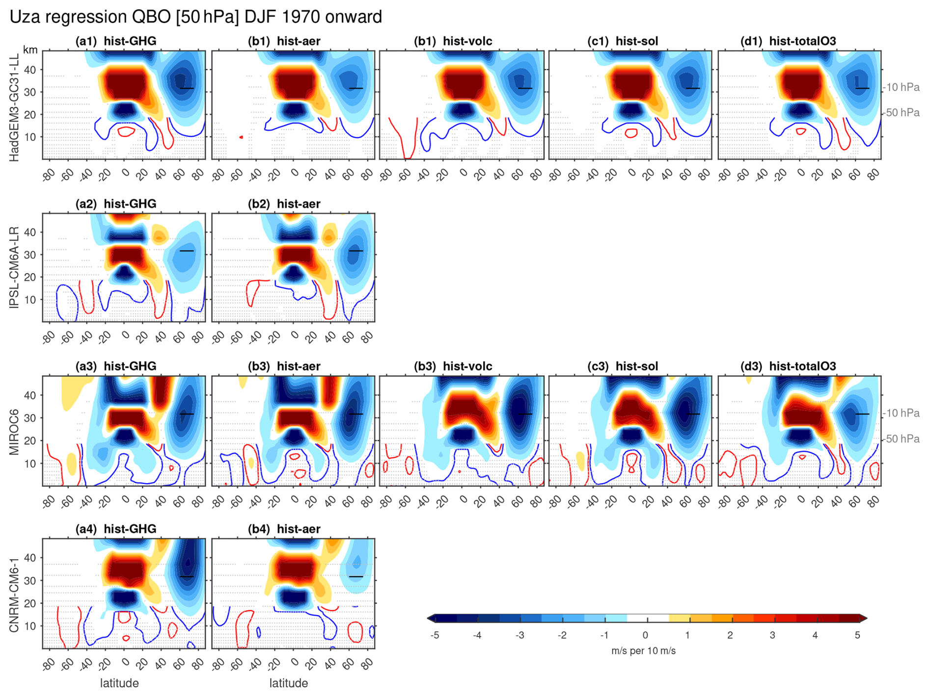
We begin by regressing the zonally averaged zonal wind and temperature against QBO50 in Figs. 1 and 2, multiplying the regression coefficients by −1 to match the sign conventions associated with an eQBO minus wQBO composite difference. By construction, strong easterlies are present in the tropical lower stratosphere and westerlies in the middle stratosphere, but robust anomalies are also evident in the extratropical stratosphere and troposphere. Remarkably, all four models simulate a H-T response in the Northern Hemisphere (NH) stratospheric polar vortex, with similar amplitudes in three of the four models (the exception is IPSL6), whereby eQBO leads to a weaker vortex. Note that intermodel differences are more pronounced if we adopt a compositing approach instead of the regression approach (Fig. S5) due to differences in QBO amplitude across the models (Figs. S1–S4). Changes in temperature in the Arctic stratosphere are also similar among HadGEM3, CNRM6.1, and MIROC6, and even the weaker response simulated by IPSL6 is highly significant (Fig. 2). In addition to the polar temperature response, subtropical temperature responses in the winter hemisphere are quantitatively similar in all four models, indicating that these models can simulate the mean meridional circulation (MMC) of the QBO.

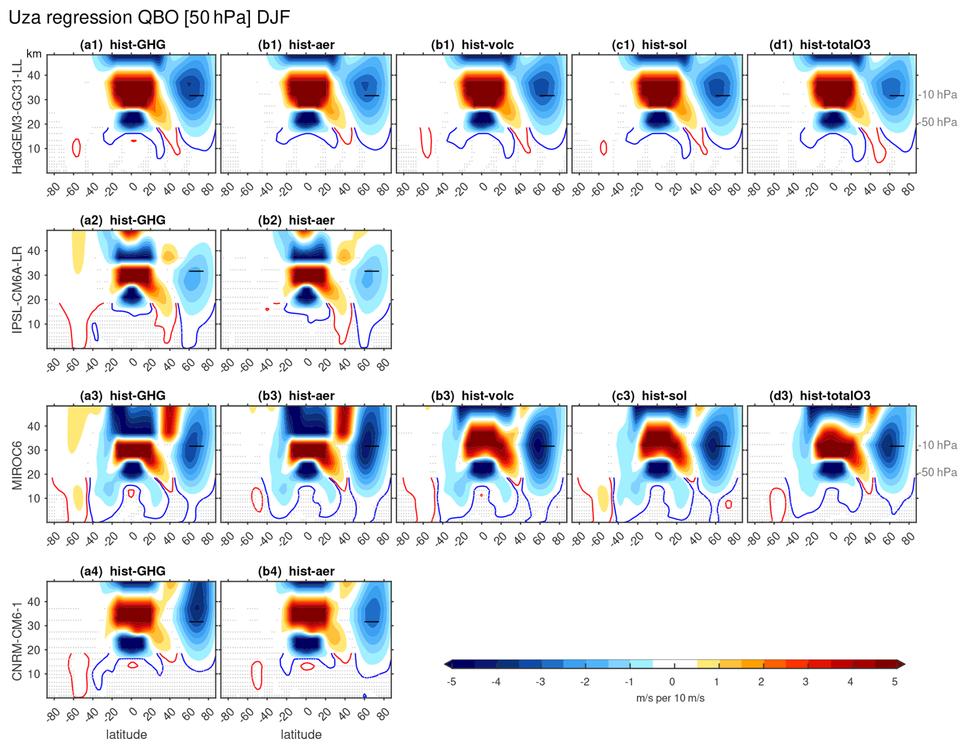
Figure 1 Zonally averaged zonal wind regressed against QBO50 in December through February. (top) HadGEM3-GC31-LL, (second) IPSL-CM6A-LR, (third) MIROC6, and (bottom) CNRM-CM6-1. All available ensemble members are included. hist-GHG is in the first column, hist-aer in the second column, hist-volc in the third column, hist-sol in the fourth column, and hist-totalO3 in the fifth column. Gray stippling indicates results are not significant at the 95 % level using a two-tailed Student's t test. The regression coefficients are multiplied by −1 to match the sign conventions associated with an eQBO minus wQBO composite difference. The black bar indicates 10 hPa from 60 to 75° N. The contour interval is 0.5 m s⁻¹ per 10 m s⁻¹ change in QBO50, and red and blue contours indicate the contour ±0.125 m s⁻¹ per 10 m s⁻¹.

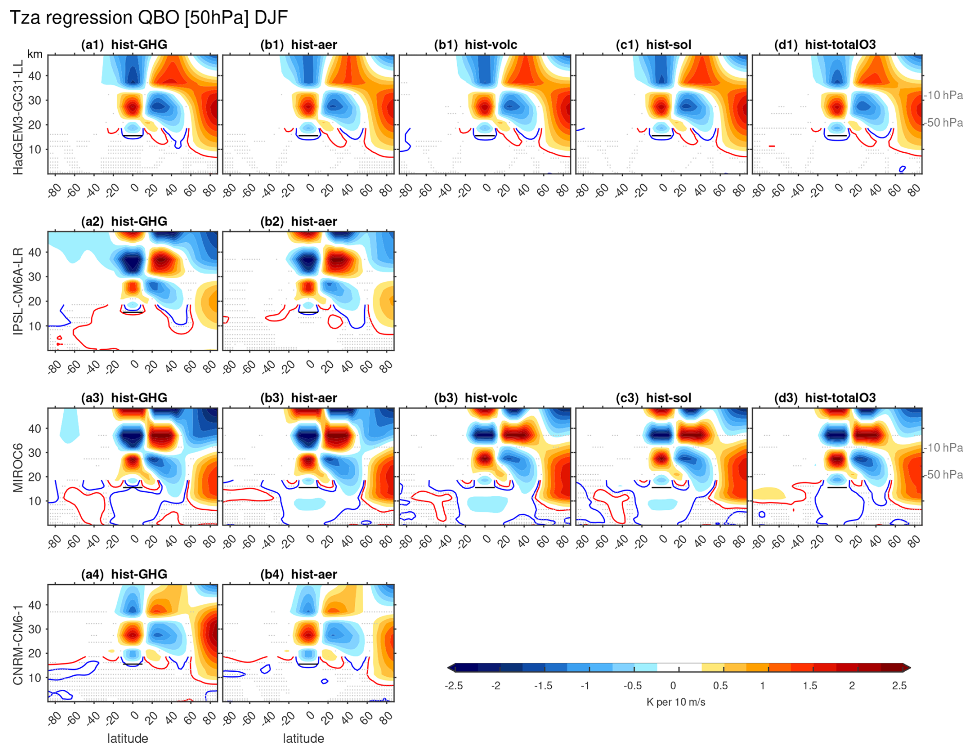
Figure 2 Zonally averaged temperature regressed against QBO50 in December through February. (top) HadGEM3-GC31-LL, (second) IPSL-CM6A-LR, (third) MIROC6, and (bottom) CNRM-CM6-1. All available ensemble members are included. hist-GHG is in the first column, hist-aer in the second column, hist-volc in the third column, hist-sol in the fourth column, and hist-totalO3 in the fifth column. Gray stippling indicate results are not significant at the 95 % level using a two-tailed Student's t test. The regression coefficients are multiplied by −1 to match the sign conventions associated with an eQBO minus wQBO composite difference. The black bar indicates 100 hPa from 10° S to 10° N as an approximation of the time-mean tropopause. The contour interval is 0.25 K per 10 m s⁻¹ change in QBO50, and red and blue contours indicate the contour ±0.0625 m s⁻¹ per 10 m s⁻¹.

As discussed in the introduction, previous work has found that CMIP-class models systematically underestimate the polar stratospheric response. The zonally-averaged zonal wind and temperature responses (analogous to Figs. 1 and 2) based on ERA5 over the period 1957 to 2023 are shown in Fig. 3. The polar vortex response in both zonal wind and temperature is quantitatively similar in ERA5 and in three of the LESFMIP models (HadGEM3, CNRM6.1, and MIROC6). On the other hand, when the vortex response is evaluated as a composite difference (Figs. S5–S7), only one model (HadGEM3) shows a vortex response close to that observed, and even HadGEM3 underestimates the amplitude of the response. This difference in conclusions between compositing and regression approaches indicates that the weaker-than-observed teleconnections in HadGEM3, CNRM6.1, and MIROC6 when using a compositing approach are due to the QBO itself being too weak in the lower stratosphere. The regression approach sidesteps this limitation, and indicates that the polar vortex response to each 10 m s⁻¹ change in QBO winds is realistic in three out of four models.

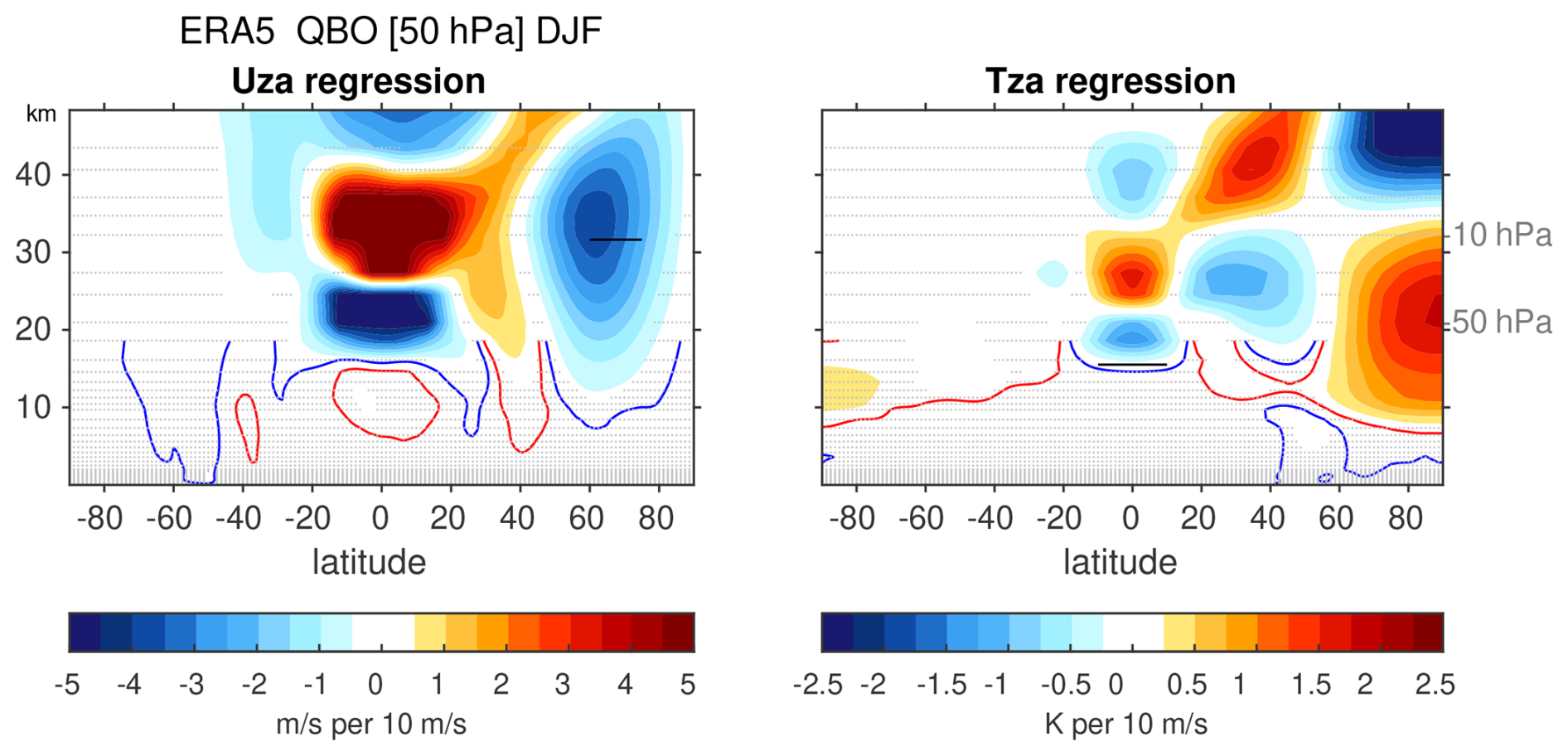
Figure 3 Zonally-averaged zonal wind and temperature regressed against QBO50 in December through February based on the ERA5 reanalysis from 1957 to 2023. Stippling indicates results are not significant at the 95 % level using a two-tailed Student's t test. Regression coefficients are multiplied by −1 to match the sign conventions associated with an eQBO minus wQBO composite difference.

The models also successfully capture other aspects of the remote response to the QBO, including the downward arching of easterly anomalies (blue contour) towards the subtropical troposphere for eQBO (3 of 4 models, the exception is IPSL6; Fig. 1) and the quadrupole temperature anomalies associated with the MMC of the QBO in the tropics and subtropical winter hemisphere (all four models; Fig. 2). The models struggle, on the other hand, with the temperature response in the equatorial lowermost stratosphere. This deficiency in the equatorial lowermost stratosphere is evident under both regression and compositing approaches, and is thus not solely a consequence of a too-weak QBO. The downward arching horseshoe is particularly pronounced in the Pacific sector (not shown). Finally, the Arctic stratospheric and downward arching horseshoe response to the QBO are weaker when the winds at 30 hPa (instead of 50 hPa) are used to define QBO phases (Figs. S8–S9).

While the winter-averaged polar stratospheric response is realistic in three of the models, there are still notable biases in the seasonality of the response. The seasonality of the Arctic vortex response is considered in Fig. 4a, which shows month-by-month regression coefficients of zonal wind at 10 hPa and 60° N against the QBO winds at 50 hPa. In the models, the vortex response peaks in February, with three of the models exhibiting no significant response in November. In ERA5, on the other hand, the response peaks in December and January, but is no longer significant in February. In all models but MIROC6, the regression coefficients in November and December are significantly weaker than those based on ERA5. Conversely, in March, the regression coefficients in HadGEM3 and in MIROC6 are significantly larger than those based on ERA5. In February, it is not possible to confidently identify a model bias when comparing with ERA5.

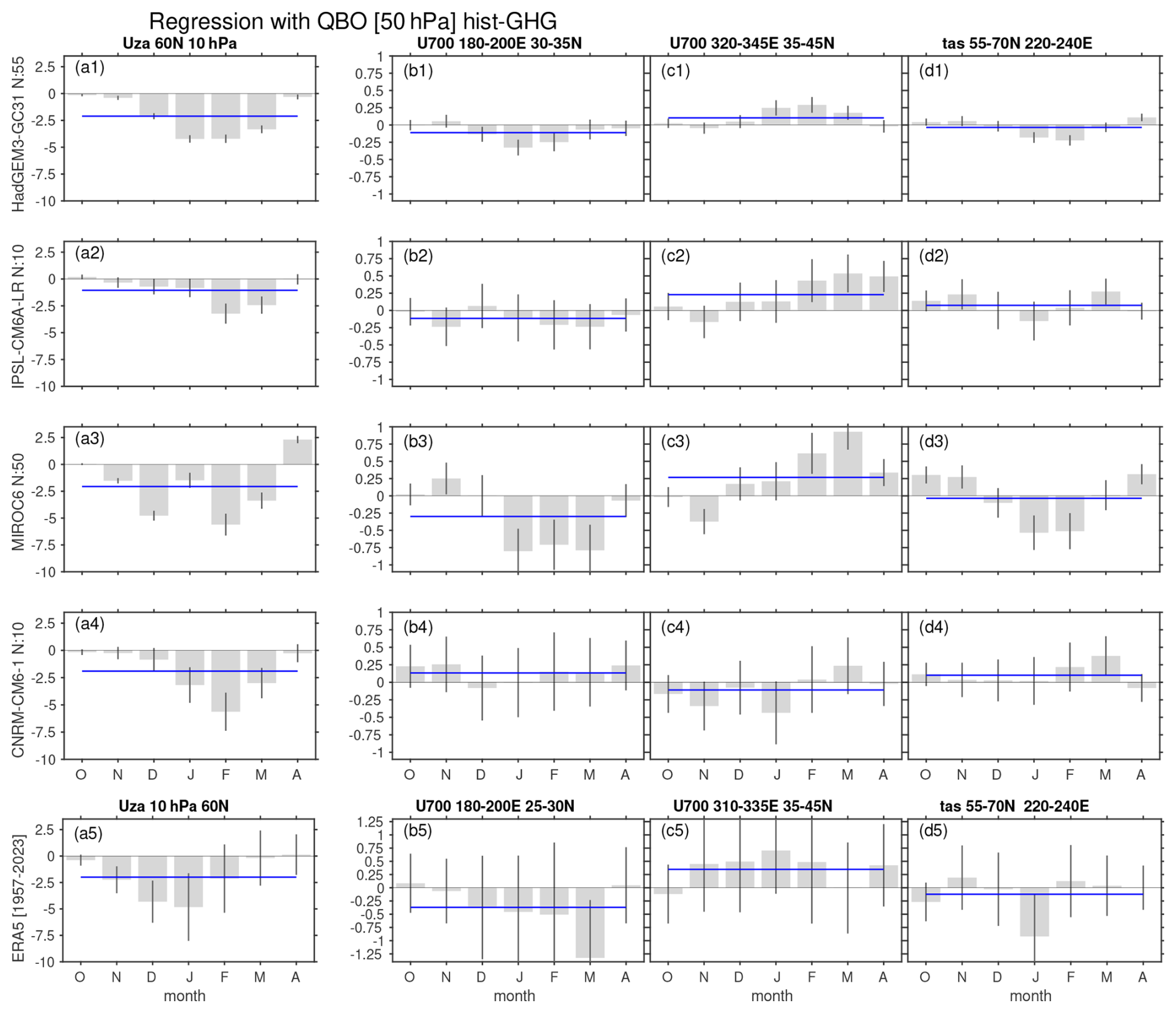
Figure 4 Seasonality of the regression of QBO50 in hist-GHG with (a) U10hPa at 60° N, (b) U700 within 30–35° N and 180–200° E (in the core of the North Pacific region, where the downward arching mechanism is most pronounced; see box on Fig. 6), (c) U700 within 35–45° N and 320–345° E (North Atlantic where the NAO response is strongest; see box on Fig. 6), and (d) surface air temperature within 220–240° E and 55–70° N (Northwest North America; see box on Fig. 7). (top) HadGEM3-GC31-LL, (second) IPSL-CM6A-LR, (third) MIROC6, (fourth) CNRM-CM6-1, (fith) ERA5 from 1957 to 2023. All available ensemble members are included. The 95 % confidence intervals on the regression coefficients are shown by vertical black lines, while the blue horizontal line shows the mean regression coefficient for October through April. For the ERA5 panels (b, c), the region selected is shifted slightly from that for the LESFMIP models to better match the regions exhibiting strong responses in ERA5. The regression coefficients are multiplied by −1 to match the sign conventions associated with eQBO minus wQBO.

A key methodological difference between our results and those from previous studies (e.g. Rao et al., 2020b) is the ensemble sizes, which are factors of 20 (for IPSL and CNRM) to 250 times (for HadGEM) larger than previous work using CMIP6 or QBOi output when aggregated across all experiments. This motivates the question as to how large of an ensemble is needed to quantify the polar vortex response. We address this question by subsampling the full large ensemble (Fig. 5). Specifically, we select with replacement 10 months in DJF from the available data, and compute the regression with zonal wind at 10 hPa and 60° N for each model and experiment. We repeat this 1000 times, and thereby generate an uncertainty estimate on the mean response. Next, we subselect 20 months and repeat 1000 times, then 30, and so until up to 25 000 randomly selected months for models with 50 ensemble members. On each panel we indicate how many months must be selected for the 2.5 % lower bounds of the uncertainty on the regression to not include 0 m s⁻¹ at 10 hPa_60N for a 10 m s⁻¹ change at U50_5S5N. At minimum, 90 DJF months are needed for HadGEM to confidently identify a significant modulation of the polar vortex, which implies that 30 years of data would be necessary. For other models, at least three times more output is necessary. However, this amount of data would still only weakly constrain the amplitude of the polar vortex response. An analogous estimate for ERA5 is provided in Fig. 5a5, which indicates that a relatively short record of only 40 months would be sufficient. This difference in the number of months required arises mainly because the vortex response in December is too weak in the models.

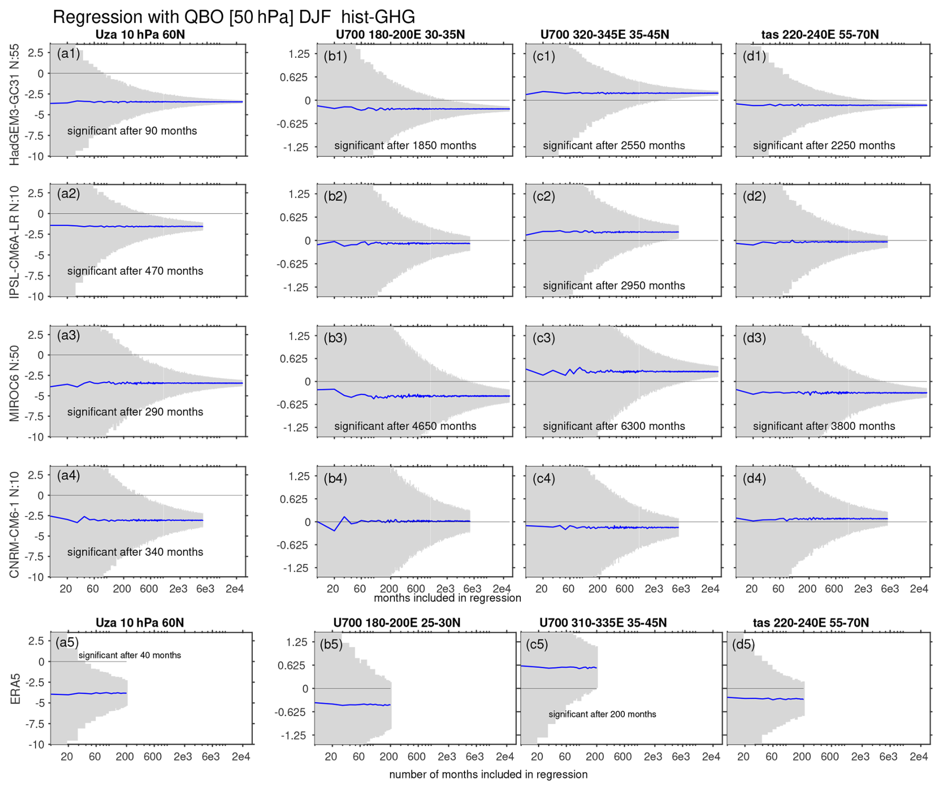
Figure 5 Regressions of QBO50 in hist-GHG in DJF with (a) U10hPa_60N, (b) U700 within 30–35° N and 180–200° E (in the core of the North Pacific region where the downward arching mechanism is most pronounced; see box on Fig. 6), (c) U700 within 35–45° N and 320–345° E (North Atlantic where the NAO response is strongest; see box on Fig. 6), (d) surface temperature within 55–70° N and 220–240° E (Northwest North America; see box on Fig. 7) upon subsampling the full ensemble to quantify the added value of a large-ensemble for quantifying teleconnection strength. (Top) HadGEM3-GC31-LL, (second) IPSL-CM6A-LR, (third) MIROC6, (fourth) CNRM-CM6-1, (fith) ERA5 from 1957 to 2023. For the ERA5 panels (b, c), the region selected is shifted slightly as compared to the LESFMIP models to better match the region with a strong response in ERA5. The regression coefficients are multiplied by −1 to match the sign conventions associated with eQBO minus wQBO. Blue lines indicate the mean of the 1000 bootstrapped samples.

We next explore the surface impacts of both the polar vortex response and the downward arching winds to the subtropical Pacific sector.

3.2 Near-surface responses

Figure 6 shows the 700 hPa zonal wind response (hereafter, U700) to the QBO. Impacts are highly robust in two regions of the NH. First, over the North Atlantic and Europe, a meridional dipole is evident that resembles the negative phase of the NAO, with an equatorward-shifted jet for eQBO relative to wQBO. Second, in the subtropical Pacific, near surface winds are weaker for eQBO than for wQBO. Both of these impacts are consistent with the observed response as discussed in previous work (see Fig. S10; e.g. Rao et al., 2020b). The Euro-Atlantic sector impacts are evident in all four models. By contrast, the impacts in the Pacific sector are most evident in HadGEM3 and MIROC6, evident to a lesser degree in CNRM6.1 (weaker and with a meridional shift), and not evident in IPSL6. This is consistent with the downward arching of QBO winds into the subtropics as represented by each model (Fig. 1). Rao et al. (2020b) also highlighted HadGEM3 and CNRM6.1 as two of the best-performing models in capturing the downward arching signal in the Pacific sector and identified IPSL6 as one of the poorer-performing models in this aspect. As reported by Rao et al. (2020b), the presence of a Pacific-sector response depends on the model's ability to capture the downward arch of QBO winds into the subtropics.

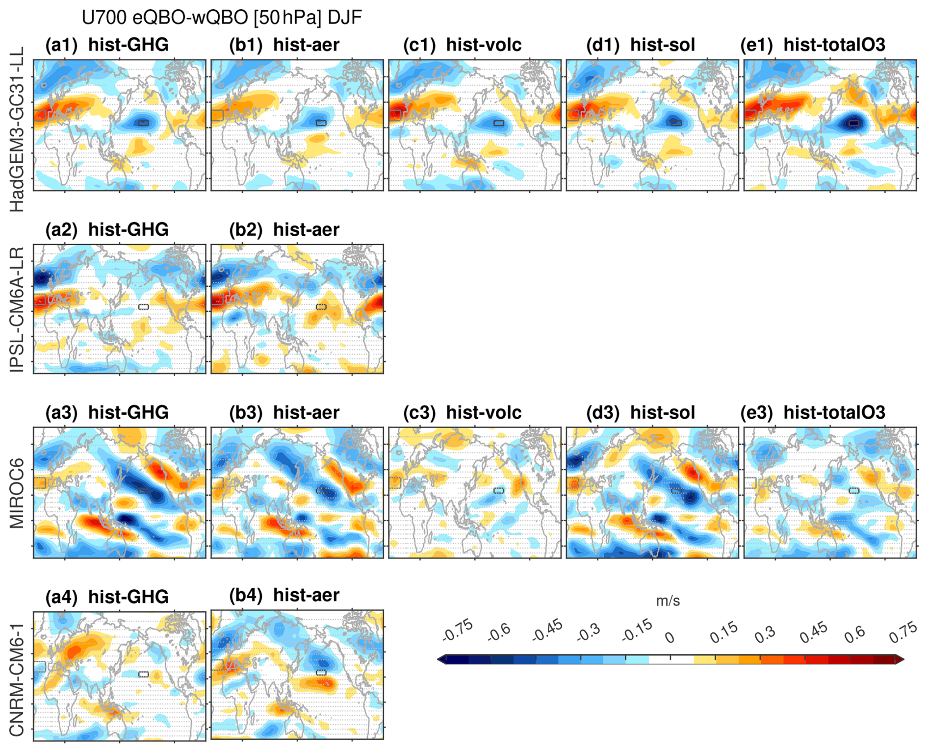
Figure 6 Difference in U700 between a composite of eQBO and a composite of wQBO months in DJF, for the QBO defined at 50 hPa. (top) HadGEM3-GC31-LL, (second) IPSL-CM6A-LR, (third) MIROC6, and (bottom) CNRM-CM6-1. All available ensemble members are included. hist-GHG is in the first column, hist-aer in the second column, hist-volc in the third column, hist-sol in the fourth column, and hist-totalO3 in the fifth column. Stippling indicates results are not significant at the 95 % level using a two-tailed Student's t test. The Atlantic and Pacific sector boxes refer to the regions used in Figs. 4b, c and 5b, c.

The downward-arching signal observed in the Pacific sector is most prominent in March, likely owing to the seasonality of the atmospheric basic state above the Pacific (Garfinkel and Hartmann, 2011a, b). Specifically, the regression coefficient from QBO50 to U700 within 180–200° E and 25–30° N (just to the south of the boxed region in Fig. 6) in ERA5 is 1.3 m s⁻¹ per 10 m s⁻¹ change in QBO50 winds in March, which is statistically significant at the 95 % level even with just 65 years of data. We assess the seasonality of this connection in Fig. 4b, which shows the regression of 700 hPa zonal winds at 180–200° E, 30–35° N (in the heart of the region exhibiting a strong response in Fig. 6) with QBO50. Both HadGEM3 and MIROC6 produce the strongest response in mid-winter, and not in March as observed. The huge amount of HadGEM3 output available allows us to conclude that this discrepancy is robust, and nearly certainly not just sampling variability. Diagnosing why the models simulate a different seasonality to the observed response is difficult with the output available on ESGF, as it would require quantitative measures of transient eddy feedbacks during different seasons based on daily fields (Garfinkel and Hartmann, 2011b).

The Atlantic-sector meridional dipole in U700 peaks in the models in February or March (Fig. 4c1–c4), while the strongest observed response is found in January (Fig. 4c5). This shift in the timing of the Atlantic sector response is consistent with the timing of the stratospheric vortex response, which is also delayed by 1–2 months in the models relative to that observed.

In Fig. 5b–c, we evaluate the size of ensemble necessary to successfully isolate the QBO impacts on U700 in the Pacific (Fig. 5b) and Atlantic (Fig. 5c) sectors using these models. In the Pacific sector, at least 1850 months (∼ 600 years) are needed before the effect can be confidently identified. Such a large sample has simply been unavailable in most previous modeling exercises. The large ensemble sizes available here allow us to constrain the magnitude of the response as estimated by these two models to be around a 0.5 m s⁻¹ change in 700 hPa zonal winds in this region of the North Pacific per 10 m s⁻¹ change in QBO50. The Atlantic sector near surface wind response has a similar magnitude and requires a similar length of data record to confidently identify a signal. Far fewer data are needed to constrain the signal in ERA5, mostly because the observed response during December is stronger in both regions than the model-simulated response. Although these signals are relatively weak, they nonetheless provide a source of predictability on annual-to-decadal timescales. We now turn to the surface temperature response to demonstrate this.

The surface temperature response to eQBO relative to wQBO (Fig. 7) is defined by warm anomalies in subtropical Eurasia and cool anomalies over much of North America and Scandinavia. This response is particularly robust in HadGEM3 but also evident in the hist-GHG runs of the other models. Subtropical Eurasian warming and Scandinavian cooling are consistent with the NAO response evident in Fig. 6. The source of the North American cooling response is more ambiguous, however, as some models also exhibit an ENSO-like response to QBO and ENSO is well-known to have a strong impact on North American temperatures (Garfinkel et al., 2019). For example, in MIROC6, eQBO is associated with La Niña and wQBO with El Niño. We first consider the nature of the relationship between the QBO and ENSO and then outline the implications for the surface temperature response.

Figure 7 As in Fig. 6 but for surface temperature. The box marks the western North America sector used in Figs. 4d and 5d.

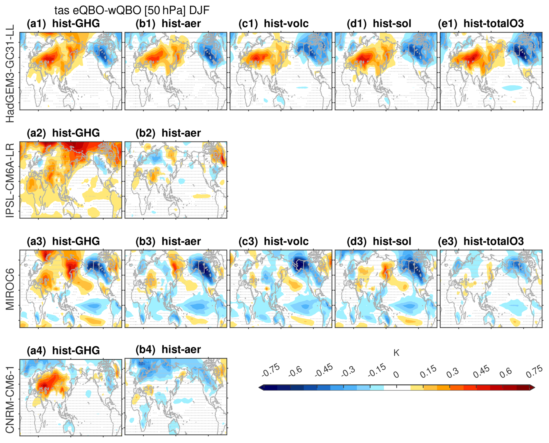
Figure 8 shows the lagged correlation of QBO50 with surface temperature in the Niño3.4 region. Correlations are essentially zero in HadGEM3 (cf. García-Franco et al., 2023), CNRM6.1, and IPSL6, however, MIROC6 simulates a statistically significant positive correlation (wQBO during El Niño). This relationship is opposite to that observed since 1950 (and similar to the single historical run analyzed by Rao et al., 2020b, their Fig. 11). These opposite responses between observations and MIROC6 are statistically robust, and indicate genuine model disagreement as to the ENSO–QBO relationship. Isolating possible mechanisms for this difference is beyond the scope of this work, however, as our primary interest is in isolating (as best as possible) the extratropical response to the QBO after regressing out any influence from ENSO.

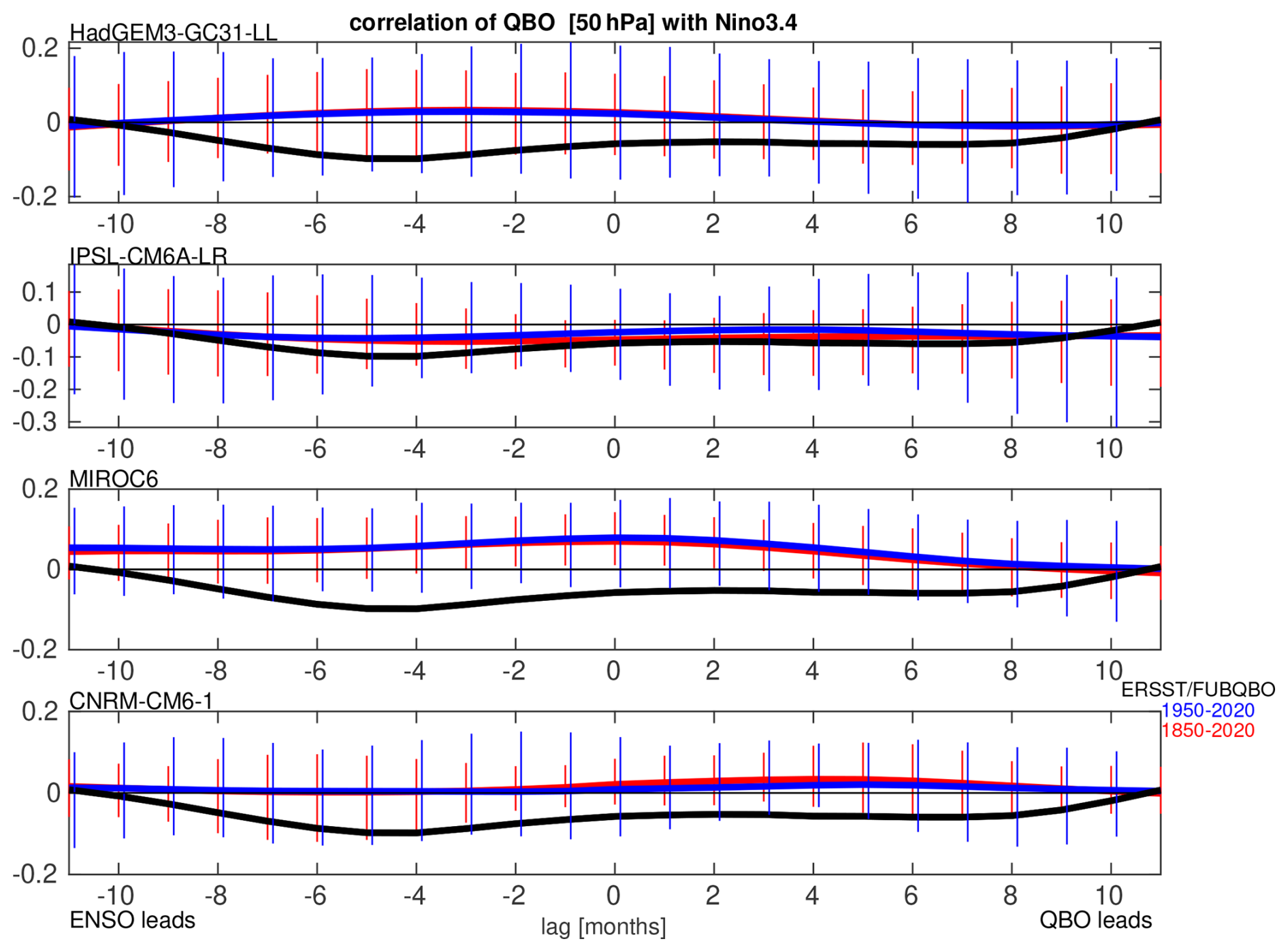
Figure 8 Lagged correlation between the QBO50 winds and the Nino3.4 index for the four LESFMIP models (averaged over all available single forcing simulations; thick lines) and for observations. The vertical lines indicate the 2.5 % to 97.5 % range of each available ensemble member. Continuous observations of the QBO only extend back to the early 1950s, and therefore we show the model correlation both over the (red) entirety of the simulations and also (blue) since 1950.

Figure 9 shows the surface temperature response to the QBO after removing linear variability associated with the simultaneous ENSO index. This adjustment yields greater agreement across models as to the magnitude and pattern of the QBO impact, though the basic pattern is similar to that shown in Fig. 7: warm anomalies over most of Eurasia, cool anomalies over Scandinavia, and cool anomalies over North America in most models and for most experiments. The cooling over North America appears to be associated with weaker westerlies in the Pacific sector, and may thus be related to reduced inland advection of relatively warm maritime air (Fig. S11).

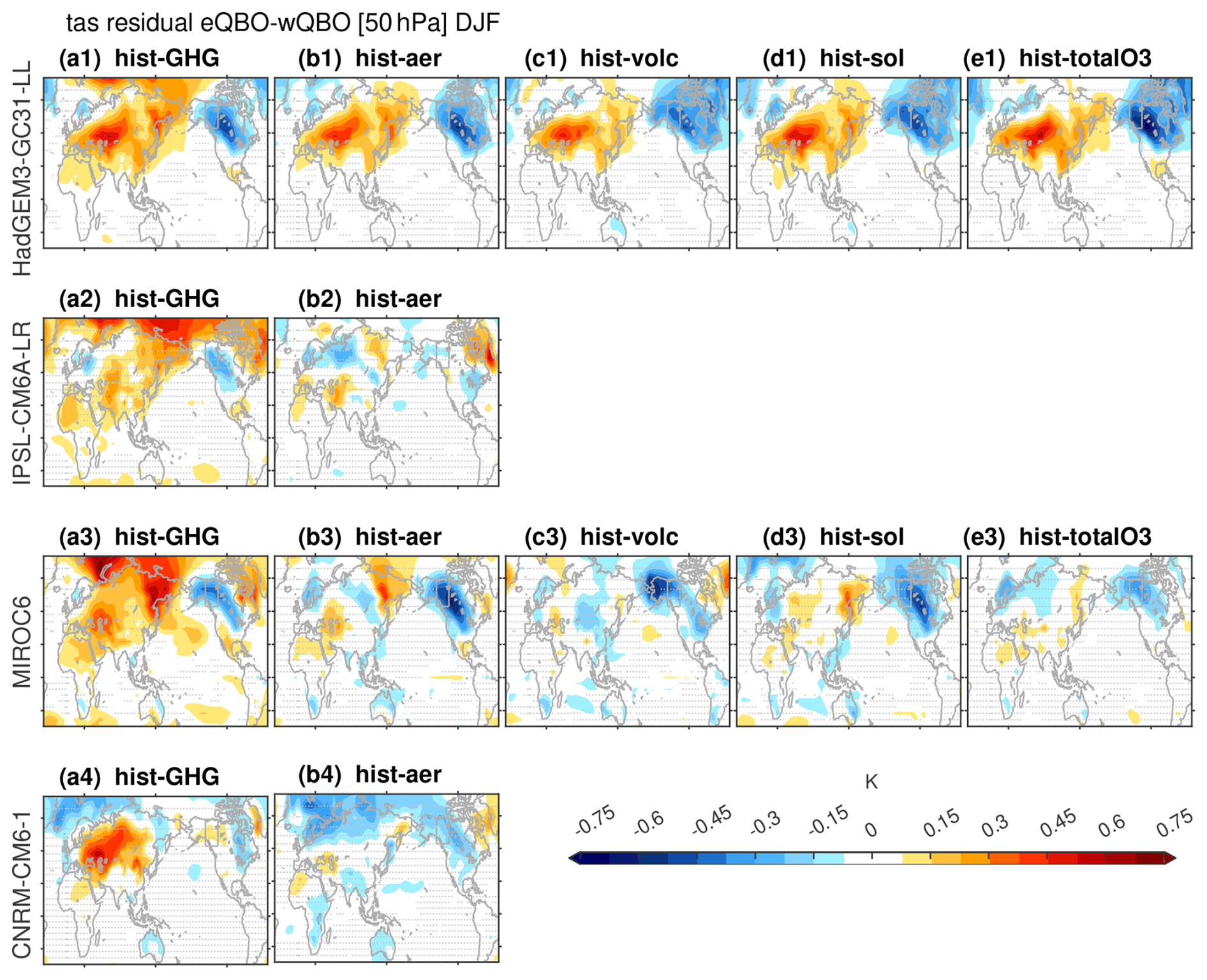
Figure 9 As in Fig. 7 but after using linear regression to exclude linear variability associated with the Nino3.4 index. The corresponding figure but for ERA5 from 1957 to 2023 is shown in Fig. S10, and for the period since 1970 in Fig. S12.

3.3 Precipitation response

We next turn our attention to the precipitation response after regressing out the linear influence of Nino3.4 (Fig. 10; the raw precipitation response evident in the eQBO minus wQBO difference is dominated by ENSO aliasing and is not shown). Precipitation increases over Western Europe and adjacent regions of the North Atlantic and decreases to the west of Scandinavia under eQBO relative to wQBO in three of the four models (with CNRM6.1 the exception). This effect is expected from the NAO-like response in U700 (Fig. 6); however, the precipitation response is shifted northward from the classical NAO response (Dai et al., 2025). Precipitation also decreases over Alaska and British Columbia for eQBO relative to wQBO, consistent with weaker westerlies in the Pacific sector (Fig. 6).

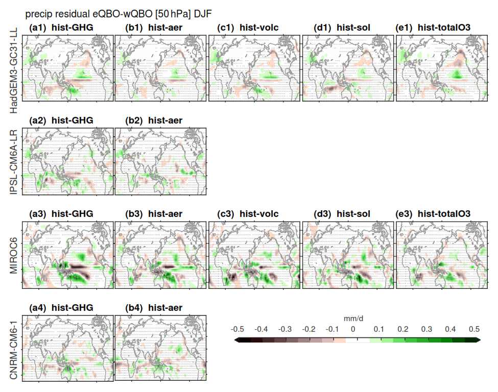
Figure 10 As in Fig. 9 but for precipitation.

Precipitation anomalies are also evident in the tropics. Despite substantial intermodel and inter-experiment spread, eQBO is generally associated with decreased precipitation in the western and central Pacific and increased precipitation along the flanks of this region. The locations and magnitudes of enhanced precipitation along the flanks of the climatologically rainiest regions vary from model to model, but are generally evident over Australia (all four models), Hawai'i (HadGEM3 and MIROC6), Southern Africa (all four models), and near the Philippines (MIROC6 and CNRM6.1). This expansion of rainy regions during eQBO (and contraction during wQBO) would not show up in zonal-mean or tropical-mean metrics of the precipitation response to the QBO. Notably, the responses shown here for the LESFMIP runs do not closely resemble those inferred from the single historical simulations analyzed by Rao et al. (2020b) (see their Fig. 8) even though the ENSO effect has been removed in the same way. Furthermore, these tropical precipitation responses are overwhelmed by ENSO aliasing if we do not regress this influence out, and we cannot rule out the possibility that other modes of tropical SST variability may also alias onto the QBO precipitation response.

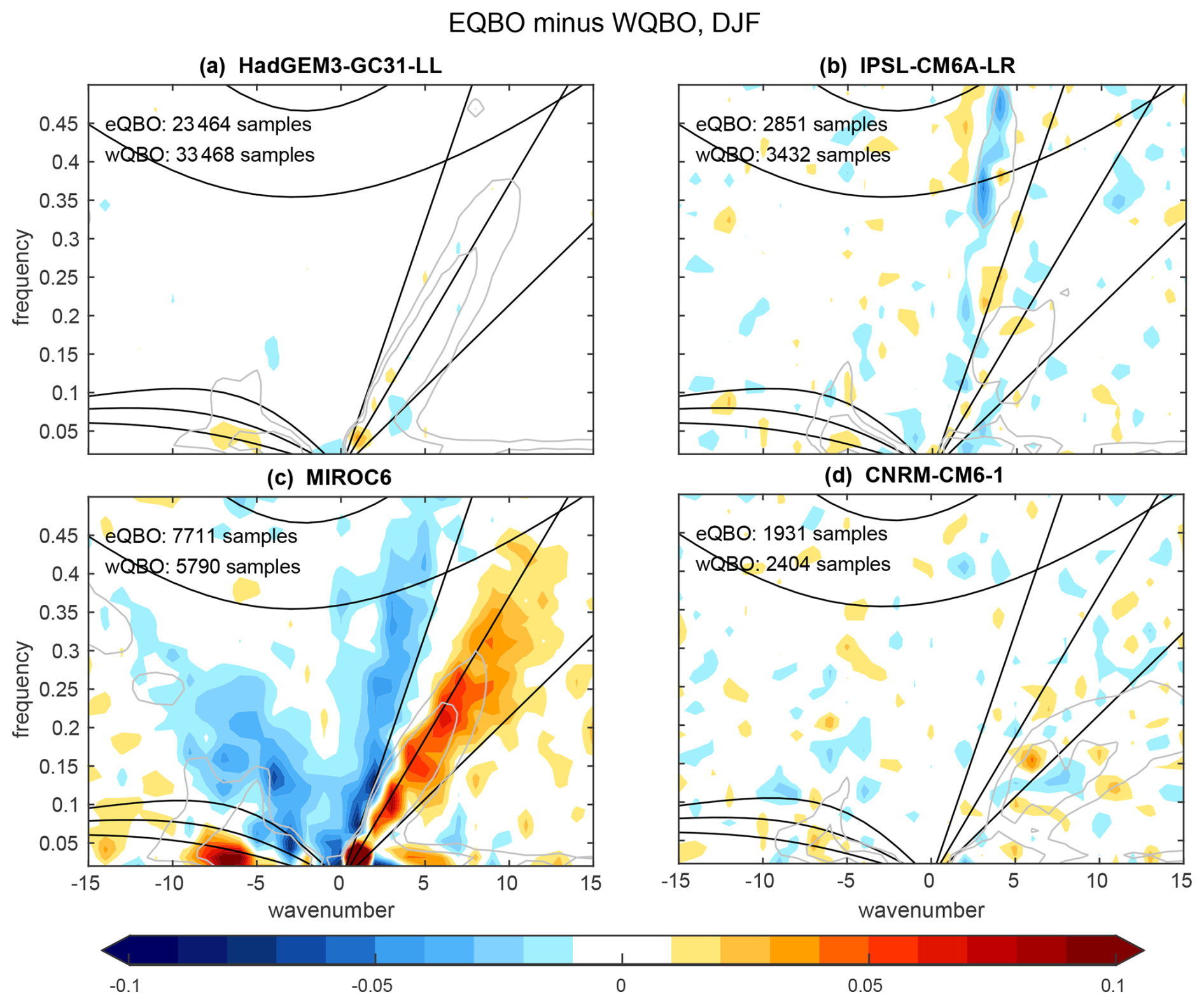
Figure 11 Symmetric spectrum of OLR under eQBO relative to that under wQBO, aggregating over all events in all available large ensemble experiments. Light gray contour lines show where the climatological spectrum for each model exceeds the background by 10 % and 20 %. Numbers of available eQBO and wQBO samples are indicated for each model in the upper left corner of the corresponding panel. See Abhik et al. (2019) for an observational analog. The MJO is characterized by wavenumbers 1 to 5 and periodicities of 20 to 70 d, and propagates to the east (positive k).

Previous work has noted that the MJO tends to be stronger under eQBO than under wQBO (Yoo and Son, 2016; Zhang and Zhang, 2018; Abhik et al., 2019; Martin et al., 2021). We use daily-mean OLR outputs to assess this relationship for each of the four LESFMIP models. After transforming to frequency–wavenumber space (see Sect. 2), we first compare the spectrum to the background spectrum for each 96 d chunk of OLR data. We then form composites of 96 d chunks in which the central date of the 96 d chunk occurs during DJF and during either eQBO or wQBO, restricting our composites to neutral ENSO conditions (Niño3.4 within ±0.5° C) to avoid aliasing.

Figure 11 shows the difference in spectra between the eQBO and wQBO composites for each model. In MIROC6, eQBO leads to a 30 % enhancement in power for wavenumber-1 for periods of 32–48 d. By contrast, wavenumber 2–3 variance is somewhat weaker for eQBO, while wavenumber 4–6 variance is 4 % stronger under eQBO. Kelvin waves are also noticeably stronger under eQBO, in agreement with Abhik et al. (2019), while higher frequency variability at small wavenumbers (large wavelengths) is generally weaker. The mean Nino3.4 indices for the eQBO and wQBO composites are indistinguishable (both −0.03 K), so this effect cannot be explained by ENSO aliasing (Fig. 8). Kim et al. (2020) found no evidence for a QBO–MJO connection in MIROC6 using 8 historical ensemble members for the period 1979–2014 (280 years of data); however here we evaluate 90 ensemble members over the full 170 years of simulation. This factor of 55 more data than used by Abhik et al. (2019) appears to isolate a signal more clearly. If we average over periods between 20 and 100 d and wavenumbers 1 to 5 (following Kim et al., 2020), the increase in MJO amplitude is 7 %. It is possible that such a signal would be missed with only 280 years of model output. Recalling that the QBO signal is too weak in the lower stratosphere, it is not surprising that MIROC6 underestimates the observed strengthening of 30 %–50 % during eQBO (Abhik et al., 2019).

The other models show little to no connection between the QBO and MJO. HadGEM3 shows a 3 % strengthening of power for wave-number one and a period of 24 d, but this effect is even weaker for longer periods and higher wavenumbers. The other two models show little effect of the QBO on equatorial wave modes, consistent with the large ensemble-based analysis of Kim et al. (2020).

Having focused thus far on boreal winter, we now turn our attention to boreal summer (June through August). Previous work using these models has indicated that they do not simulate a connection between the QBO and the South Asian monsoon (Hu et al., 2024); however, the LESFMIP provides orders of magnitude more data than was previously available. Figure 12 shows the response to eQBO as compared to wQBO after regressing out the linear relationship with the Nino3.4 index. In all experiments, precipitation increases either over South Asia (HadGEM3, IPSL6, MIROC6) or East Asia (CNRM6.1) for eQBO relative to wQBO. There are substantial intermodel and inter-experiment differences in other regions, however, and as for DJF we cannot rule out aliasing from other SST modes of variability. Furthermore, these precipitation signals in JJA tend to not be statistically significant unless more than 10 ensemble members are available, and so require more than 15 000 years of output to stand out from the noise. This may be due, in part, to the too-weak response of equatorial temperature to the QBO at 100 hPa (Fig. 2).

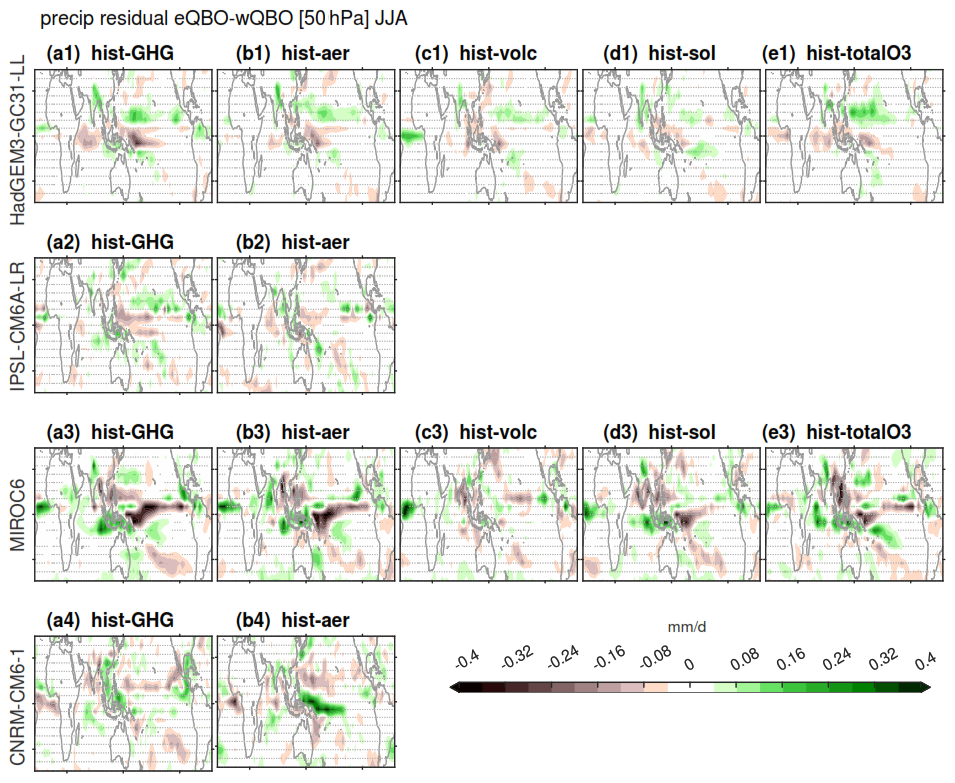
Figure 12 As in Fig. 10 but for JJA.

4 Sensitivity of teleconnections to external forcings

The LESFMIP data allows for an unprecedented examination of the ability of external forcings to affect the strength of QBO teleconnections. Previous work has found that the polar vortex response to the QBO strengthens in a future climate with increased GHGs even as the QBO itself weakens (Rao et al., 2020c, 2023), and we now revisit this effect by examining the response in the hist-GHG experiment for the period since 1970 (Fig. 13). Although regression coefficients between the QBO winds and winds at 10 hPa and 60° N increase by 7 %, this increase is not statistically significant in individual models, however it is robust across models. When evaluated as a composite difference, on the other hand, the teleconnection strength weakens in 2 of 4 models (Fig. S5), likely due to weakening of the QBO in response to increased GHGs (Garfinkel et al., 2025). The downward arching winds to the subtropical troposphere also strengthen after 1970, with the regression coefficient between the QBO and U700 over the North Pacific increasing by 15 % in the multi-model mean (Fig. S11). HadGEM and MIROC6 (the two models that better capture this relationship) show even larger increases. However, these increases still do not reach the level of statistical significance despite the enormous amount of data in individual models. The cold anomaly over northwestern North America is also 36 % stronger after 1970 in HadGEM and MIROC6 (Figs. 9, S12). This difference barely misses the threshold for statistical significance at the 95 % level and is significant at the 90 % level. In contrast, the Atlantic sector U700 response shows no strengthening after 1970. Overall, the intensification of QBO teleconnections in response to increased GHGs is more pronounced in the Pacific sector via the downward arching subtropical horseshoe than in the North Atlantic via the polar stratosphere.

Figure 13 As in Fig. 1 but for the period since 1970.

To understand why the subtropical horseshoe strengthens, we turn to thermal wind balance on an equatorial β-plane upon applying L'Hopital's Rule (Sect. 8.2 of Andrews et al., 1987) and the thermodynamic equation (Sect. 7.2 of Andrews et al., 1987):

$$\begin{array}{}\text{(1)}& {\displaystyle \frac{\partial u}{\partial z}}=-{\displaystyle \frac{R}{H\mathit{\beta }}}{\displaystyle \frac{{\partial }^{\mathrm{2}}T}{\partial y^{\mathrm{2}}}}\text{(2)}& {\displaystyle \frac{\partial T}{\partial t}}+\mathit{v}\cdot \mathrm{\nabla }T+{\displaystyle \frac{H{N}^{\mathrm{2}}}{R}}{\stackrel{\mathrm{‾}}{w}}^{*}=-{\displaystyle \frac{T-T_{\mathrm{eq}}}{\mathit{\tau }}}\end{array}$$

Assuming a quasi-steady state and weak horizontal temperature gradients (both $\frac{\partial T}{\partial t}$ and v⋅∇T are near zero), vertical shear of the zonal wind must be balanced by a temperature anomaly, which in turn must be balanced by vertical motion. Static stability decreases near the tropopause and in the lower stratosphere under increased GHGs (Vallis et al., 2015) regardless of the QBO. This reduced static stability under climate change necessitates a stronger vertical velocity, and hence a stronger mass circulation, to achieve the same temperature anomaly to balance the vertical shear of the zonal wind. This point is demonstrated explicitly in Fig. S13: for each 10 m s⁻¹ strengthening of easterly QBO winds at 50 hPa, the upwelling anomaly in $\stackrel{\mathrm{‾}}{w^{*}}$ at 60 hPa doubles at the end of the hist-GHG experiment as compared to the beginning, and this effect is still evident for $\stackrel{\mathrm{‾}}{w^{*}}$ at 90hPa (∼ 50 % increase at the end of the hist-GHG experiment). This increase in vertical velocity per m s⁻¹ change in QBO wind necessitates a corresponding increase in the meridional velocity of the QBO's MMC due to mass continuity, including in the MMC in the vicinity of the tropopause. The Coriolis torque from this increase in near-tropopause meridional velocity induces a larger zonal wind anomaly in the subtropical upper troposphere in the presence of elevated GHGs, in turn altering eddy activity and the tropospheric jets (Garfinkel and Hartmann, 2011a, b).

There is little agreement across models as to whether elevated aerosol concentrations since 1970 affected surface teleconnections. Teleconnections are weaker in HadGEM3 under hist-aer but stronger in MIROC6 and CNRM6.1 (Figs. S11 and S12). In hist-volc, simulated QBO teleconnections are stronger in the 1880s (Krakatoa) and 1990s (Pinatubo) in MIROC6 but weaker during those same decades in HadGEM3 (not shown). Sensitivities of QBO teleconnections to the solar cycle will be evaluated in an upcoming paper. Finally, prescribed time-evolving ozone leads to stronger surface teleconnections in the Pacific sector wind response but weaker surface teleconnections in the Atlantic sector using HadGEM3, but weaker teleconnections in both regions using MIROC6 (Figs. 6e and 9e). Prescribed ozone changes invigorate the QBO winds in both models (Kataoka et al., 2020; Butchart et al., 2023; Garfinkel et al., 2025), and so the stronger teleconnections in HadGEM are more in line with expectations. Restricting the analysis to after 1970 (the era with ozone depletion) has little impact (Figs. S11e and S12e).

5 Discussion and Summary

The Quasi-Biennial Oscillation (QBO) can be skillfully predicted months or even years in advance (Pohlmann et al., 2013; Scaife et al., 2014; Stockdale et al., 2020). Because the QBO can influence climate outside of the tropical stratosphere, the predictability of the QBO offers a potential for improved predictability in several key regions on seasonal to multi-annual timescales. Previous work has found that QBO teleconnections tend to be too weak in models (Elsbury et al., 2021; Rao et al., 2020b; Garfinkel et al., 2018; Andrews et al., 2019; Anstey et al., 2021). The recent availability of large ensembles from models with spontaneously-generated QBOs allows us to revisit and refine this conclusion.

The results demonstrate that the biggest contributor to this under-estimate is that the QBO is too weak in the lowermost stratosphere in nearly all models (Rao et al., 2020a; Richter et al., 2020). It is therefore important to consider the possibility that too-weak teleconnections are a byproduct of biases in the QBO itself rather than biases in the mechanisms that connect the QBO to remote regions. This possibility can be evaluated by regressing climate variables in remote regions onto QBO winds. This approach sharpens focus on the teleconnection mechanisms while side-stepping issues in the QBO amplitude, while compositing approaches could conflate the two.

All four models show a Holton–Tan effect linking the QBO to the polar stratosphere (Figs. 1 and 2), with regression results indicating that the amplitude of this effect is similar to that observed in three of the four models. By contrast, a compositing approach yields a pronounced underestimate (Fig. S5) due to the weaker-than-observed QBO amplitude in all models (Figs. S1–S4), a common model bias that is nonetheless difficult to fix (Garfinkel et al., 2022) though not insurmountable (Schwartz et al., 2026). The Holton–Tan response is consistent with a meridional dipole in zonal wind in the North Atlantic sector (Fig. 6), anomalies in surface temperature over most of Eurasia (Fig. 7), and a meridional dipole in precipitation anomalies over Europe (Fig. 10). These effects are to be expected, given the well-known role of the polar stratosphere in regulating the NAO (Baldwin et al., 2021; Scaife et al., 2022).

The large ensemble sizes also allow for clarifying the QBO level which most strongly affects the vortex. Both the Arctic stratospheric response and the downward arching horseshoe response to the QBO are weaker when winds at 30 hPa (instead of 50 hPa) are used to define QBO phases (Figs. S8–S9; Andrews et al., 2019). We therefore recommend using 50 hPa winds to define the QBO when possible. The large ensemble sizes also allow us to confidently identify a delay in the Holton–Tan effect by a month or two in models (peaking in February) relative to observations (Fig. 4a). Likewise, the simulated Holton–Tan effects are weaker than observed in November and December. This delay in the Holton–Tan effect leads to a corresponding delay in the Atlantic sector and Eurasian surface responses (Fig. 4c). These discrepancies stand out more clearly in our study than in any previous work due to the huge amount of data examined. Despite these discrepancies, this study confirms a genuine influence of the QBO on the North Atlantic sector as represented by these models (Andrews et al., 2019).

All four models simulate a subtropical temperature response in the winter hemisphere quantitatively similar to that observed, indicating that these models can simulate the MMC of the QBO. However, the models underestimate the temperature response in the equatorial lowermost stratosphere (Fig. 2). This underestimate in the equatorial lowermost stratosphere is evident regardless of whether a regression approach or a compositing approach is used, and is therefore not solely a consequence of a too-weak QBO.

The models also successfully capture other aspects of the remote response to the QBO, including the downward arching of easterly wind anomalies towards the troposphere in the subtropics during eQBO (in 3 models, with IPSL6 the exception; Fig. 1) and the cold tropical TTL anomalies associated with eQBO's MMC (all four models; Fig. 2). This effect is particularly pronounced in the Pacific sector (Fig. 6), however, the models simulate the largest impact in mid-winter, rather than in March when the observed effect peaks (Fig.4b). These Pacific sector wind anomalies affect surface temperature and precipitation over western North America (Figs. 7 and 10). This impact of the QBO on North American temperature and precipitation does not appear to have been noted before and, while present in ERA5 data (Fig. S10), it is not statistically significant. We expect that as the observational record lengthens, the signal may begin to emerge. One of the models also simulates a robust connection between the QBO and ENSO (Fig. 8), however these remote teleconnections are robust even after regressing out the (linear) ENSO influence.

Precipitation anomalies are also evident in the tropics, but with substantial intermodel and inter-experiment spread. In DJF, eQBO leads to precipitation expanding away from the region with strongest precipitation climatologically, in contrast to contraction of these regions during wQBO. In JJA, precipitation increases in the core Southeast monsoon region in eQBO relative to wQBO. However, inter-model and inter-experiment differences in both JJA and DJF indicate that the precipitation response to the QBO is poorly constrained even when using large ensembles, and may instead reflect genuine model differences (Schwartz et al., 2026). Furthermore, these precipitation signals are typically not statistically significant unless more than 10 ensemble members are available, and so require more than 15 000 years of output to stand out from the noise. The relative weakness and scattered nature of these precipitation signals likely is a consequence of the QBO amplitude being too weak in the lowermost stratosphere, and particularly the too-small response of temperature near the tropical tropopause (Fig. 2; Schwartz et al., 2026). Finally, these tropical precipitation responses are overwhelmed by ENSO effects if we do not regress these influences out, and we cannot rule out the possibility that other modes of tropical SST variability also alias into the QBO precipitation response.

One model (MIROC6) simulates the observed relationship between the QBO and the MJO (Fig. 11). Despite the effect being weaker than observed, this model is remarkably more successful than previous CMIP-class models in reproducing this teleconnection. Future work is needed to constrain the regions in which this signal is most pronounced, and to more fully explore why this model is relatively more successful than the others.

Finally, the Holton–Tan mechanism strengthens (though not significantly in individual models) in response to increased GHGs when evaluated as a regression (in agreement with Rao et al., 2020c, 2023), but not when evaluated as a composite difference. This sensitivity of the conclusions to the precise methodology can be attributed to the weakening of the QBO in response to increases in GHGs (Garfinkel et al., 2025). The downward arching wind response in the subtropical Pacific sector also strengthens after 1970 in the hist-GHG experiment, likely because the QBO's lower stratospheric MMC strengthens in response to a reduction of lower stratospheric static stability forced by increased GHGs (Fig. S13). Other external forcings have no clear impacts on teleconnections that are robust across models.

Overall, the use of large ensembles has allowed us to develop a clearer picture of how well models simulate QBO teleconnections while revealing surface impacts over North America that appear to not have been noticed before. Some previous claims that models systematically underestimate QBO teleconnections are likely the result of insufficient sample size or the use of a compositing approach to evaluate teleconnections, which mixes together the well-known bias in QBO amplitude in the lower stratosphere with biases in the processes that connect QBO winds with remote regions. Regardless, there remain important biases in the timing of the teleconnections, and individual models show pronounced biases in the surface responses even after accounting for the relative weakness of the QBO in the lower stratosphere.

Despite these persistent biases, our results indicate that the QBO in better-performing models can already be used to improve surface climate predictability on seasonal to multi-annual timescales. However, it is critically important to improve the representation of the QBO in the lowermost stratosphere in all models. Without a realistic QBO in this region, teleconnections will need to be bias corrected to account for systematic underestimation of the lower stratospheric signal, potentially contributing to surface expressions of the signal-to-noise paradox (O'Reilly et al., 2019; Weisheimer et al., 2024).