Predictability of extreme surface weather associated with Mediterranean cyclones in ECMWF ensemble forecasts – Part 1: Method and case studies

Extratropical cyclones are the main cause of extreme surface weather events in the Mediterranean such as heavy precipitation, floods, severe winds, and dust storms. However, the accuracy in predicting the timing, location, and intensity of such events is often insufficient, which is typically related to errors in cyclone position, propagation, and intensity. In this two-part study we use operational ensemble forecasts from the European Centre for Medium-Range Weather Forecasts to quantify the predictability of extreme surface weather conditions linked to Mediterranean cyclones. We apply an object-based approach to attribute events of extreme precipitation and surface winds to Mediterranean cyclones. Thereby, objects of extreme surface weather are identified at grid points that exceed the seasonal 99th percentile of these parameters and matched to cyclones based on their distance to the cyclone center. In this first part, we introduce the probabilistic method and three illustrative case studies of Mediterranean cyclones that occurred between November 2022 and September 2023, including the infamous Storm Daniel as well as Storms Denise and Jan. We find that the cyclones as well as their attributed objects of extreme surface weather are predicted well for lead times ≤ 48 h. However, for longer lead times there is large case-to-case variability in the ensemble performance. Predictions of extreme surface weather objects are found to be more uncertain (i) for smaller and less coherent objects, (ii) if the associated cyclone is captured by fewer ensemble members, and (iii) during the earlier stage of the cyclones' lifecycle. The methodological development and its application documented in this paper provide the basis for a multi-year investigation of the predictability of extreme weather linked to Mediterranean cyclones in the second part of this study.

1 Introduction

Early on, the Mediterranean has been identified as an active cyclogenetic region with hot spots of cyclone formation in the Gulf of Genoa in the western and near Cyprus in the eastern Mediterranean, respectively (e.g., Gleeson, 1953; Pettersen, 1956). Mediterranean cyclones develop mostly due to baroclinic instability with their evolution often being affected by the complex topography surrounding the Mediterranean Sea and by diabatic processes (Trigo et al., 1999; Flaounas et al., 2022). Their occurrence has a significant seasonal cycle with a notable increase in more intense and longer-lived cyclones in winter (Lionello et al., 2006; Campins et al., 2011; Flaounas et al., 2018). Although Mediterranean cyclones are typically weaker, smaller, and shorter-lived than extratropical cyclones in the main storm track regions (Trigo, 2006; Čampa and Wernli, 2012; Flaounas et al., 2014), they are the major cause of extreme surface weather events in the Mediterranean, including heavy precipitation and floods, severe winds and dust storms (e.g., Pfahl and Wernli, 2012; Raveh-Rubin and Wernli, 2015; Flaounas et al., 2022). Jansà et al. (2001) found that over 90 % of heavy rainfall events in the western Mediterranean occur within 600 km of a cyclone center. Surface wind extremes are found to be almost always related to a cyclone (Nissen et al., 2010; Raveh-Rubin and Wernli, 2015), as are compound precipitation-wind extremes (Raveh-Rubin and Wernli, 2015; Portal et al., 2024). Due to the dense population of the Mediterranean region, cyclones that are attributed to extreme surface weather can cause severe environmental and socio-economic damage (e.g., EUMETSAT, 2018; FloodList, 2022; WMO, 2023; Khodayar et al., 2025).

To adequately prepare for extreme Mediterranean weather, improve early-warning systems, and issue measures such as evacuation procedures in time, it is essential to evaluate recent versions of forecast models. The predictability of Mediterranean cyclones in the ensemble forecast and reforecast products of the European Centre for Medium-Range Weather Forecasts (ECMWF) has been assessed in several studies, concluding that Mediterranean cyclones can be accurately predicted by the ensemble, but only few days in advance (Pantillon et al., 2017; Di Muzio et al., 2019; Vollenweider, 2023). For longer lead times, a systematic underestimation of cyclone propagation speed and intensity has been found (Pantillon et al., 2017). Furthermore, improved forecasts of the cyclone location were found to be linked to slower and more shallow cyclones (Doiteau et al., 2024). This agrees with the findings of Froude et al. (2007a), who further showed that in general, the “forecast skill for the position of extratropical cyclones is significantly higher than for their intensity”. Despite the poorer forecast performance for rapidly intensifying cyclones and the resulting less accurate prediction of winter cyclones in the Mediterranean, Doiteau et al. (2024) could show that the more intense a cyclone is, the more ensemble members actually detect this cyclone compared to shallower cyclones. Furthermore, Di Muzio et al. (2019) showed that ensemble forecasts typically cannot predict medicanes, a category of particularly severe Mediterranean cyclones (e.g., Fita et al., 2007; Di Muzio et al., 2019), further ahead than 5 to 7 d, a result that is consistent with the existence of predictability barriers (Riemer and Jones, 2014; Pantillon et al., 2016). They also revealed that forecasts initialized after the formation of the cyclone are distinctively more accurate than earlier forecasts, which still need to capture the cyclogenesis process.

While several studies investigated the predictability of cyclones in the main storm tracks (e.g., Froude et al., 2007b; Froude, 2010; Zheng et al., 2017; Korfe and Colle, 2018; Büeler et al., 2023), the predictability of Mediterranean storms has been studied to a lesser extent. In particular, forecasting the timing, location and intensity of Mediterranean cyclones associated with extreme surface weather has often been found to be insufficiently accurate (e.g., Davolio et al., 2015). The catastrophic flooding of the city of Derna, Libya, attributed to Storm Daniel in September 2023 (e.g., CBS News, 2023; Greek Reporter, 2023; WMO, 2023; Armon et al., 2025) is one example that emphasizes the need for accurate predictions of such storms.

The predictability of cyclone-attributed extreme rainfall and surface winds varies substantially from case to case (e.g., Pantillon et al., 2017). Several studies showed that the forecast performance is sensitive to both the structure and amplitude of upper-level potential vorticity (PV) anomalies as well as to the interaction of the low-level flow with the complex Mediterranean topography and, in particular, to the position and intensity of the surface cyclone (Fehlmann and Quadri, 2000; Romero et al., 2005; Argence et al., 2009; Horvath and Ivančan-Picek, 2009). Simulating a heavy rainfall event, Argence et al. (2009) found that initial perturbations applied to an upper-level trough intensified throughout the simulation, resulting in forecast discrepancies of the low-level cyclone. They further showed that the overall precipitation pattern was controlled by both the upper-level PV structure and the cyclone at the surface. However, the predictability of smaller-scale features such as localized heavy precipitation was found to be directly related to the forecast of the location and/or intensity of the surface low (Romero et al., 2005).

This two-part study investigates the prediction of extreme surface weather conditions linked to Mediterranean cyclones in the operational ECMWF ensemble prediction system (ENS). The goal of Part 1 of this study is to present a method to identify Mediterranean cyclone-related surface weather extremes in ENS. We illustrate the method with three contrasting case studies and conduct some initial analysis on the predictability of surface weather extremes and their link to cyclone characteristics. While our method is based on several pragmatic choices to ensure its feasibility, it can be applied quasi-operationally to ensemble forecasts and allows for systematically quantifying probabilities of forecasting extreme surface wind and precipitation related to Mediterranean cyclones at different lead times, which – to the best of our knowledge – has not been done before.

Results from a statistical multi-year investigation will be presented in Part 2 (currently in preparation) of this study. Applying our method to a large set of Mediterranean cyclones and their associated extremes will allow us to draw more robust conclusions about the link between the predictability of these extremes and cyclone characteristics such as their position, intensity, and propagation speed. Furthermore, we aim to investigate in future studies how the predictability of extreme surface weather conditions in the Mediterranean is influenced by upstream processes over the North Atlantic, e.g., a warm conveyor belt influencing Rossby wave breaking over Europe (Raveh-Rubin and Flaounas, 2017; Scherrmann et al., 2024).

This paper is organized as follows. We present the datasets and methods used in Sect. 2, followed by an introduction of three case study cyclones and their representation in ERA5 in Sect. 3. In Sect. 4, we analyze the performance of ENS, in particular the representation of the cyclone track and attributed objects of extreme surface weather in the forecasts at different lead times. We discuss our results and conclude the study in Sect. 5.

2 Data and method

This study uses two different datasets from ECMWF, namely the ERA5 reanalysis and medium-range ensemble forecasts (ENS) produced with the ECMWF Integrated Forecasting System (IFS), which are briefly introduced in Sect. 2.1 and 2.2. Then, we present the methodological steps required to address the research questions outlined in the introduction. These steps are:

1. Identification and tracking of Mediterranean cyclones as 2-dimensional objects in ENS, and matching with cyclones in ERA5 (Sect. 2.3).

2. Identification of 2-dimensional objects of extreme surface precipitation and 10 m wind gusts (Sect. 2.4).

3. Attribution of extreme surface weather objects to cyclone objects (Sect. 2.5).

4. Analysis of ensemble forecast probabilities of extreme surface weather objects (in a cyclone-centric framework; Sect. 2.6).

2.1 ERA5 reanalysis

The ERA5 reanalysis (Hersbach et al., 2020) is used as a reference dataset for forecast validation, featuring a 1-hourly temporal resolution and interpolated to a grid with a spatial resolution of 0.5° × 0.5°. To make the dataset comparable to ENS (see Sect. 2.2) we only use 6-hourly data in this study. Mean sea level pressure (SLP) is used to identify cyclones, while fields of total precipitation (P) and 10 m wind gusts (G₁₀) are utilized to identify objects of extreme surface weather. A 30-year climatology from 1990–2019 is considered to define thresholds for extreme events (see Sect. 2.4). Furthermore, in Sect. 3, the large-scale environment of the case study cyclones is investigated with fields of potential temperature (θ) at 850 hPa and potential vorticity (PV) on isentropic levels.

2.2 Operational IFS ensemble forecasts (ENS)

Twice per day, at 00:00 and 12:00 UTC, the ECMWF runs 50 medium-range ensemble members with slightly perturbed initial conditions and stochastically perturbed parameterization tendencies during the forecast integration. For each initialization time, we keep a 6-hourly forecast output that is available up to a maximum lead time of 15 d. Since May 2022, we have been retrieving several fields from these forecasts quasi-operationally with full vertical resolution on the 68 lowest model levels in a domain covering North America, Greenland, the North Atlantic, Northern Africa, and Europe (130° W–80° E and 15–80° N), on a horizontal grid with 0.5° grid spacing¹. The operational model versions since the start of the download have included IFS Cycles 47r3, 48r1 and 49r1. While the consideration of different IFS Cycles is unavoidable for this study, we expect that the predictability signal is generally stronger than systematic differences between the different cycles. Due to the substantial storage capacities that would be needed to keep this data, many of the subsequently described object-based postprocessing steps are also performed quasi-operationally twice a day before archiving parts of the data on our servers and eventually on tape. Nevertheless, a selection of atmospheric fields is stored, including temperature, wind, moisture and precipitation, and additionally calculated secondary parameters such as θ and PV. This continuously growing dataset allows us to assess current ensemble prediction capabilities of extreme weather events and associated dynamical features for a multi-year period.

We specifically chose to establish and analyze this unique operational dataset instead of reforecast data. Using operational forecast data provides us not only with more ensemble members, which likely improves the quality of the ensemble spread. Operational forecasts are also run with a higher native spatial resolution, which might be particularly relevant when looking at small-scale extremes. Furthermore, the availability of the full three-dimensional model level data allows us to expand our analysis and investigate, for example, the role of upper-level PV and upstream processes on the forecast performance of Mediterranean cyclones. Given that one month of downloaded (about 7 TB) and post-processed data (about 12 TB) takes together about 19 TB of storage space, the size of our dataset will soon exceed 400 TB – figures showing that using a higher spatiotemporal resolution would no longer be feasible. However, the many ensemble members and the long lead times provide us with 1500 d of forecast data per day of download, which, together with the inclusion of model level data, results in a unique and extensive dataset to investigate aspects of atmospheric predictability in the North Atlantic and European region.

Given the conceptual and technical challenges of applying our method to operational ensemble forecasts and visualizing the results, in particular because of the large amount of data and analyses involved, it requires a careful introduction. For instance, for a single cyclone in ECMWF's ERA5 reanalysis (ERA5), considering the corresponding ensemble forecasts twice daily with 50 members each and lead times up to 10 d, requires the identification of the cyclone and its attributed extreme weather objects in 1000 individual forecasts.

2.3 Cyclone identification, tracking, and cyclone track matching

Extratropical cyclones are identified in ERA5 and in each ensemble member of ENS as two-dimensional objects (Wernli and Schwierz, 2006). Thereby, a cyclone is defined as the area around a local minimum in SLP, bounded by the outermost closed SLP contour. To identify cyclone tracks, the algorithm presented in Sprenger et al. (2017) is applied. A cyclone track has to exist for at least 24 h to be considered. Mediterranean cyclones are identified as cyclones that reach their mature stage, i.e., their minimum central SLP, within a “Mediterranean box” extending from 10° W to 40° E and 30 to 47° N (except for the Bay of Biscay in the northwestern corner). A seasonal climatological Mediterranean cyclone frequency is calculated as the spatial average of the seasonal cyclone frequency at each grid point in this box. Note that to make both datasets comparable, cyclone tracks in ERA5 (which are based on hourly SLP fields) are only considered every 6 h, i.e., at 00:00, 06:00, 12:00 and 18:00 UTC.

To investigate the ability of the ENS members to predict an observed cyclone track as identified in ERA5, a cyclone track matching algorithm is applied for Mediterranean cyclones similar to Flaounas et al. (2023) as illustrated in Fig. 1a. For each Mediterranean cyclone track in ERA5, the following criteria are applied to identify matching cyclone tracks in each ENS member:

• Spatial criterion. At a certain time step, the location of the cyclone center in an ensemble member has to be within a radius of 300 km around the cyclone center in ERA5 to be regarded as a match.

• Temporal criterion. For a cyclone track in an ensemble member to be matched with an ERA5 cyclone track, the spatial criterion has to be fulfilled for at least three consecutive time steps, that is a minimum of 12 h. Note that this period is shorter than the one used by Flaounas et al. (2023), who applied this method to compare different tracking methods within the identical dataset as opposed to the matching of cyclone tracks between reanalyses and forecasts in our case.

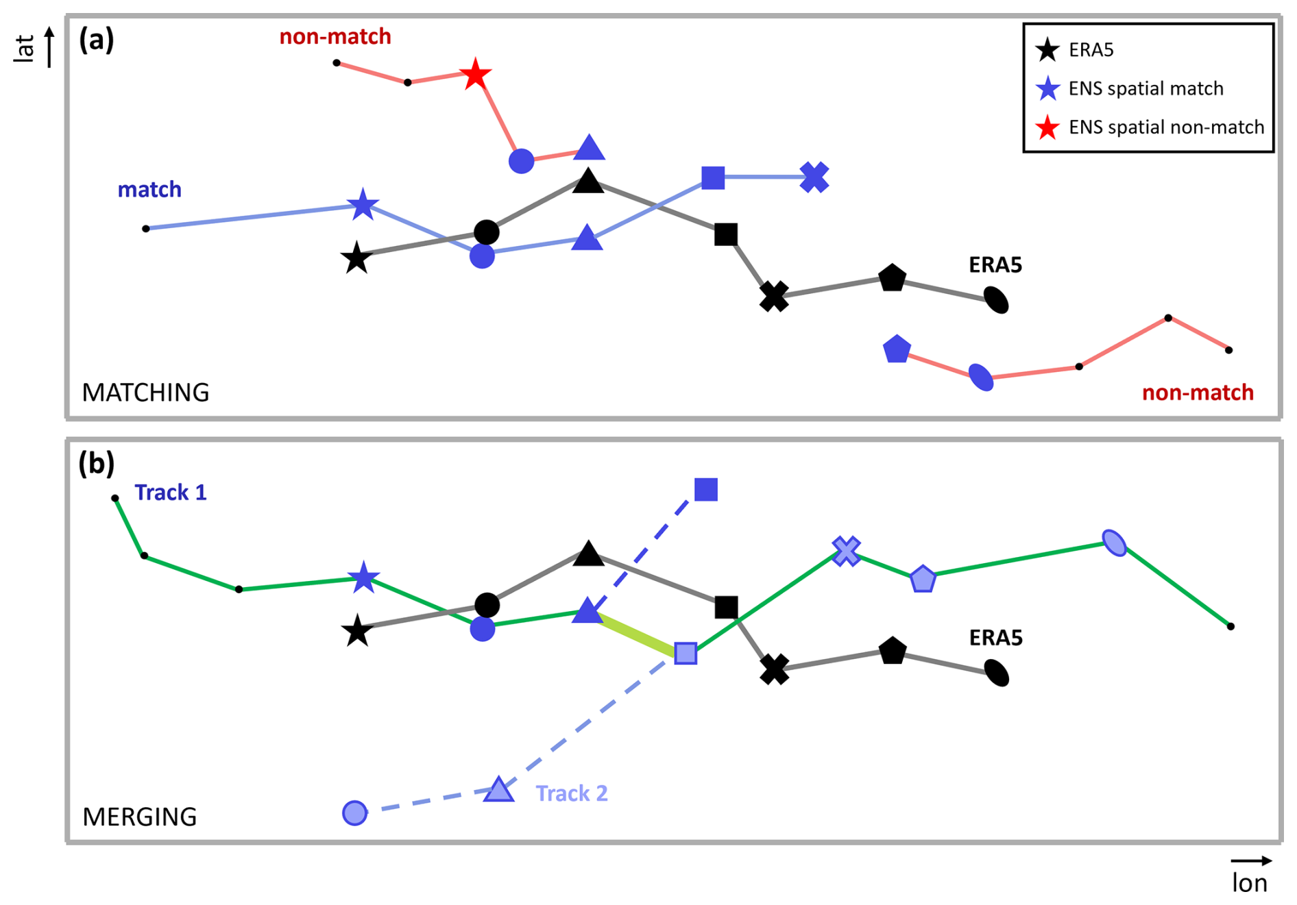
Figure 1 Schematic of the cyclone track (a) matching and (b) merging algorithms. Black line denotes a cyclone track in ERA5, colored lines denote tracks in an ensemble member. Identical symbols refer to the same 6-hourly time step. Blue symbols and lines denote time steps and tracks, respectively, that match the spatial criterion, and red symbols and lines situations that do not match the spatial and/or temporal criterion. In panel (b), both blue tracks were identified in the same member. Dashed lines denote the original tracks, and the green line denotes the merged, final track. Light green line denotes the artificial “connector” merging the original tracks.

With this choice of criteria, the number of matching tracks per time step along the ERA5 cyclone track can vary considerably, particularly for longer cyclone tracks. It is further possible that more than one matching cyclone track is found in a single ensemble member, either because of a gap in the identified cyclone track or due to the presence of two cyclones in the forecast. Such cases are more common for cyclones with a longer lifetime, which often feature one cyclone in ENS matching the ERA5 track in the earlier stage and the second one in the later stage of the ERA5 cyclone. Depending on the lead time this occurs in up to 36 % of all members of our case studies (see Sect. 2.7). To avoid the occurrence of two matching tracks in the same ensemble member at the same time step, the matching tracks are merged to a single track as shown in Fig. 1b, considering only the ensemble member track point closest to the ERA5 track. The resulting merged tracks compare well with tracks in members featuring only one track (not shown).

2.4 Definition of extreme surface weather objects

To investigate the performance of ENS in predicting extreme surface weather attributed to the identified cyclones, we define two-dimensional objects of extreme precipitation and extreme surface wind gusts as follows. First, a threshold is determined at each grid point based on the 99th percentile of 6-hourly accumulated P (P₉₉) and the maximum G₁₀ within a 6 h period (G_10, 99) in the ERA5 reanalysis dataset. The percentiles are determined separately for each season, i.e., for December to February, etc. (see Fig. S1 in the Supplement). Although it would be preferable to similarly use an ENS-based percentile threshold for the analysis of extreme weather objects in ENS, this is not practical, given the challenge to obtain an operational IFS model climatology without downloading an extensive amount of additional hindcast data. Therefore, we pragmatically use the thresholds defined in ERA5 also for ENS. In a next step, adjacent grid points that exceed P₉₉ and G_10, 99, respectively, are defined as extreme surface weather objects described by a two-dimensional binary field with a value of 1 at grid points inside the object, and 0 outside. Thereby, only grid points with values of P ≥ 2 mm and G₁₀ ≥ 20 m s⁻¹ are considered, respectively. In this way, coherent regions of intense P and G₁₀ are objectively identified in the ERA5 reanalysis as well as in each ENS member. In the following, we will refer to such objects as “extreme objects”.

2.5 Attribution of extreme objects to cyclones

Extreme objects are attributed to surface cyclones based on the following objective approach: If at a certain time step an extreme object overlaps with the circle spanned by a radius of 400 km around the cyclone center, the entire extreme object is attributed to the cyclone. In a study by Portal et al. (2024), such a threshold distance was found to be reasonable to identify precipitation extremes attributed to surface cyclones in the Mediterranean. Portal et al. (2024) further showed that surface wind extremes attributed to a surface cyclone usually extend to areas more distant from the cyclone center. However, to avoid an overlap of extreme objects attributed to different cyclones, we choose to apply the same threshold for both extreme P and G₁₀. Furthermore, in case of merged tracks (see Sect. 2.3), we only attribute extreme objects for track points that are within a radius of 1000 km around the ERA5 cyclone center to avoid accounting for objects that cannot be linked to the cyclone.

We are aware that our methods to match and merge cyclone tracks in ENS as well as to define and attribute objects of extreme surface weather are based on pragmatic choices and comparatively simple criteria. While this certainly implies limitations, it is necessary to keep our methodology feasible given the amount of data and technical effort involved (as explained in Sect. 2.2). Furthermore, a pragmatic framework will allow for an easier application of our method to other datasets.

2.6 Probability of extreme objects

To assess the performance of ENS in forecasting extreme objects relative to a surface cyclone, a cyclone-centered probability of the occurrence of such objects in ENS (hereafter referred to as “probability of extreme objects”) for a given forecast and lead time is calculated at each time step along the ERA5 track, as shown in Fig. 2. In a first step, for each ensemble member, all extreme objects within a box of ±10° relative to the cyclone center as represented in this ensemble member are collected (illustrated exemplarily for five ensemble members in Fig. 2a–e). A value of 1 is attributed to all grid points within an extreme object. Members without a matching cyclone contribute with a constant field of 0 to the overall probability. In a second step, taking the mean over all 50 ensemble members results in the probability of an extreme object near the cyclone center in ENS (Fig. 2g, h).

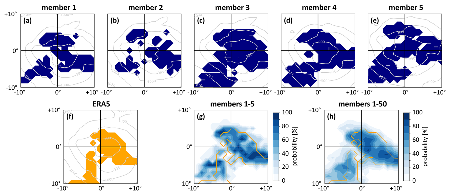
Figure 2 Illustration of the calculation of cyclone-centered probabilities of the occurrence of extreme objects in ENS. Panels (a)–(e) show cyclone-centered extreme objects (dark blue shading) and SLP fields (grey contours; in intervals of 5 hPa) for five randomly selected members; panel (f) shows the extreme object (orange) and SLP field at same time step in ERA5. Panel (g) depicts the average of panels (a)–(e), i.e., the object probability for the five ENS members (blue shading; in %) and the ERA5 object (orange contour). Panel (h) shows object probability including all 50 ENS members.

2.7 Case study selection

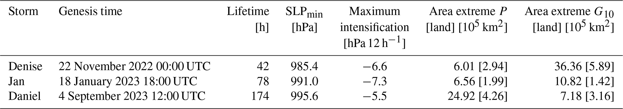
In this paper, three case studies are performed to illustrate our methodology of quantifying the performance of ENS in forecasting extreme surface weather attributed to Mediterranean cyclones. The case studies are chosen based on the occurrence of such extreme weather events since the start of our systematic ENS evaluation in May 2022. Also, the cases are chosen such that they represent different types of Mediterranean cyclones, which helps testing the methodology across the spectrum of cyclones with different characteristics. Key characteristics of the cases are summarized in Table 1. Case study 1 (Storm Denise) investigates a classical lee cyclone in the Gulf of Genoa (Tafferner, 1990; Buzzi et al., 2020); case study 2 (Storm Jan) a cyclone that propagates from the North Atlantic into the western and central Mediterranean, with a track similar to Storm Klaus (Liberato et al., 2011); and case study 3 (Storm Daniel) an exceptionally long-lived cyclone in the eastern Mediterranean that developed medicane characteristics (Flaounas et al., 2025). First, we introduce the three storms using ERA5 reanalysis data before analyzing their representation in ENS.

Table 1 Characteristics of all three case study storms in ERA5, including their genesis time, lifetime, minimum SLP (SLP_min), their maximum intensification (SLP decrease) in 12 h, and the total affected area of P and G₁₀ extremes (affected land area in brackets), respectively, integrated along the cyclone track.

3 Case study overview

3.1 Case study 1: Storm Denise – November 2022

The first case study investigates Storm Denise, which formed at 00:00 UTC on 22 November 2022 in the Gulf of Genoa, causing severe wind gusts, high waves and storm surge over Mallorca and Corsica (Majorca Daily Bulletin, 2022; European Severe Weather Base, 2022). During 22 November it passed over northern Italy where it reached its minimum SLP of less than 990 hPa at 12:00 UTC, leading to strong winds and heavy precipitation mainly in the Emilia-Romagna region (FloodList, 2022) before reaching the coast of Croatia on 23 November, where extreme winds were observed along the Adriatic coast (European Severe Weather Base, 2022). Several fatalities were reported in Italy, mainly related to a landslide that was partially triggered after the passage of the storm (Agenzia Italia, 2022; CNN World, 2022). Cyclolysis already happens 42 h after genesis, such that this is the cyclone with the shortest lifetime but lowest SLP minimum among the three cases (Table 1).

Associated areas of extreme P and G₁₀ in the ERA5 dataset are shown in Fig. 3. Colors do not indicate the intensity of the extremes, but their duration at a given grid point. For instance, a number of 3 track points with an extreme object indicates that at this location the extreme conditions attributed to the same cyclone persisted for 18 h (three 6-hourly time steps). While extreme P occurred mainly during the intensification stage of the cyclone (Fig. 3a), attributed extreme G₁₀ affected large parts of the Mediterranean Sea and especially Italy and Corsica, covering the largest areas near the time of the cyclone's mature stage at 12:00 UTC on 22 November (Fig. 3b). Compared to the two other cases, the area affected by extreme winds is more than 3 times larger, which is coherent with Storm Denise showing the lowest minimum central SLP of all three storms (Table 1).

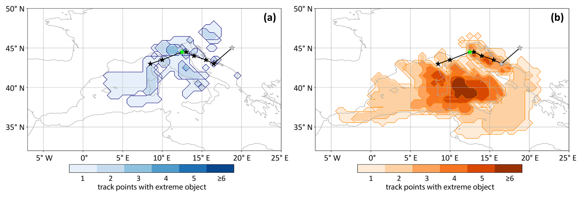
Figure 3 Track of Storm Denise (black line) with 6-hourly objects of extreme (a) precipitation and (b) surface wind gusts in ERA5. Shading indicates the number of 6-hourly track points with overlapping extreme objects at each grid point. Single track points are denoted every 6 h by black stars if they are attributed to an object and by grey stars if no object occurs at that time step. Green star marks time and location of maximum cyclone intensity (minimum SLP).

Figure 4 shows the synoptic situation during cyclogenesis and the mature stage of Storm Denise. A pronounced trough over France and Germany extends towards the western Mediterranean Sea where it initiates lee cyclogenesis south of the Alps at 00:00 UTC on 22 November. At this time, both extreme P and G₁₀ occur near the cyclone center and behind the cold front, which can be seen in maps of θ at 850 hPa (Fig. 4b). Twelve hours later, when the cyclone reaches its minimum SLP, the upper-level trough is developing into a cyclonic PV streamer with maximum PV values south of the cyclone center (Fig. 4c). While extreme P still occurs close to the cyclone center and the cold front, extreme G₁₀ extends over a large area mainly south of the cyclone center, reaching parts of the North African coast (Fig. 4d).

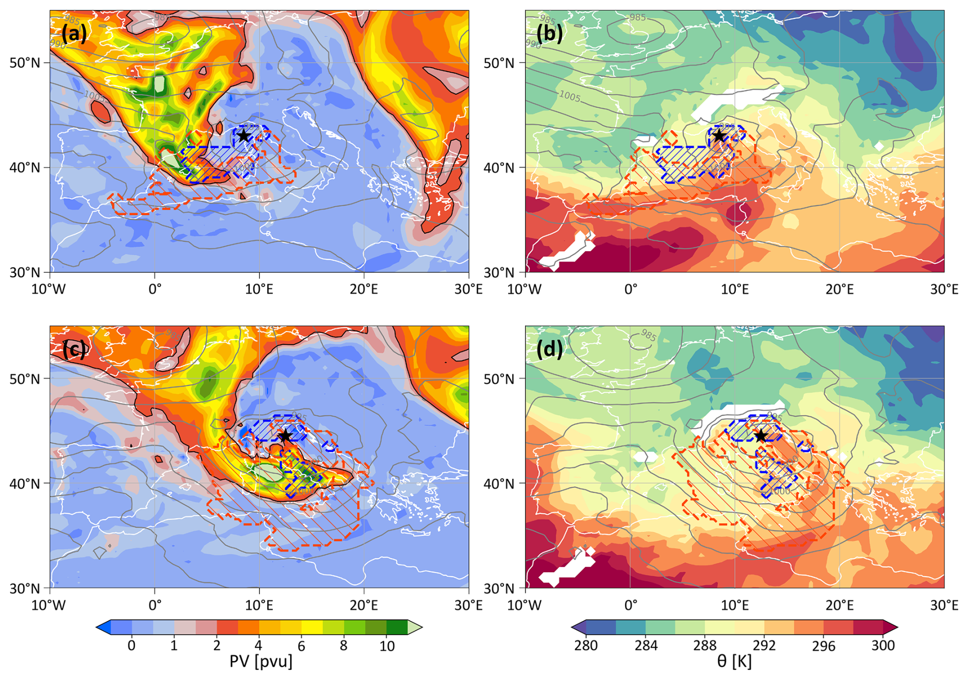
Figure 4 Maps of (a, c) PV on 315 K (color; in pvu) and (b, d) θ at 850 hPa (color; in K) at (a, b) 00:00 UTC on 22 November (time of cyclogenesis) and (c, d) 12:00 UTC on 22 November (time of minimum SLP, 12 h after genesis). Cyclone center is marked by black star. Areas of extreme precipitation and surface wind gusts are shown with blue and orange hatching, respectively. Grey lines denote SLP in intervals of 5 hPa.

3.2 Case study 2: Storm Jan – January 2023

In January 2023, genesis of Storm Jan happened over the North Atlantic at 18:00 UTC on 18 January. On 20 January it passed along the northern edge of the Pyrenees towards the Mediterranean, where it intensified by 10 hPa in 18 h before reaching its maximum intensity of 991 hPa ahead of the Italian coast near Naples at 18:00 UTC on the same day. On the following day, Storm Jan experienced a small re-intensification over the Adriatic Sea before undergoing cyclolysis at 00:00 UTC on 23 January. After causing high winds in France and Spain, the storm affected particularly Italy and the Balkans with strong wind gusts and heavy snowfall (AEMET, 2023; European Severe Weather Base, 2023).

Extreme objects were diagnosed only when the storm reached the European continent as shown in Fig. 5. Reaching the Mediterranean, extreme precipitation affected Sardinia and central Italy (Fig. 5a), while extreme surface winds occurred mainly south of the cyclone center over the sea (Fig. 5b). Figure 6 shows two time steps when large areas were affected by extreme P and G₁₀, occurring close to the mature stage of the cyclone. The surface cyclone is positioned below a pronounced large-scale trough that stretches from Spain towards Greece (Fig. 6a, c). At both time steps, extreme P occurs near the cyclone center and an area of extreme G₁₀ extends to the southwest. While extreme winds overlap with an area of warm air at 06:00 UTC on 20 January (Fig. 6b), they occur mainly behind the cold front 12 h later (Fig. 6d).

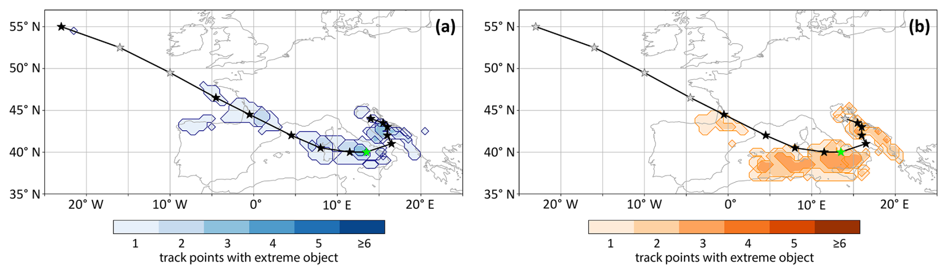
Figure 5 Same as Fig. 3 but for Storm Jan.

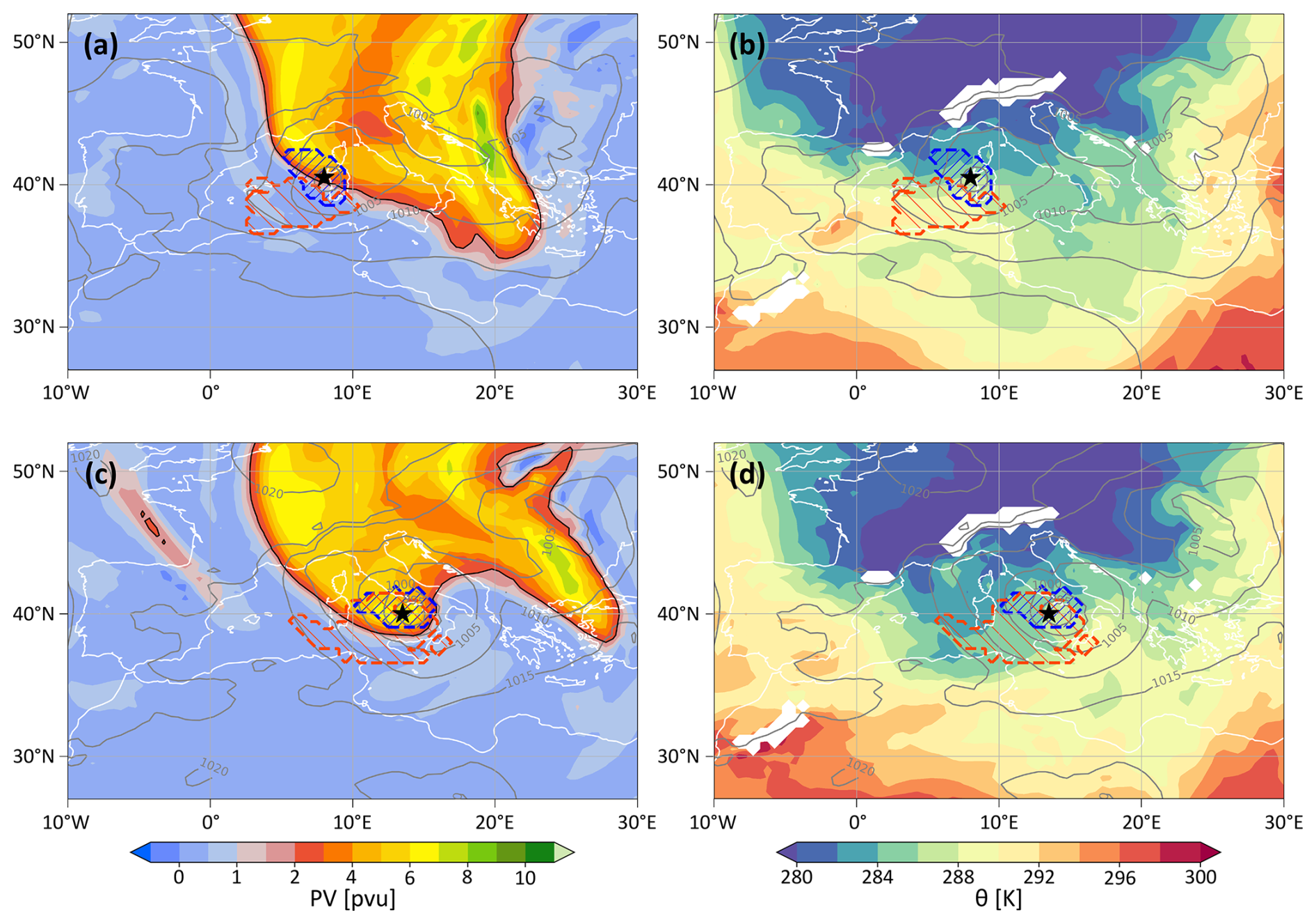
Figure 6 Same as Fig. 4 but for Storm Jan at (a, b) 06:00 UTC on 20 January (36 h after genesis) and (c, d) 18:00 UTC on 20 January (time of minimum SLP, 48 h after genesis). PV maps show PV at 310 K.

3.3 Case study 3: Storm Daniel – September 2023

At the beginning of September 2023, Storm Daniel hit the headlines as it caused extreme rainfall and devastating floods in parts of Greece and, a week later, northern Libya. Storm Daniel formed at 12:00 UTC on 4 September off the west coast of Greece. After causing severe flooding in Greece following a first intensification stage on 5 September (AP News, 2023; CBS News, 2023; Greek Reporter, 2023), the cyclone became stationary in the Ionian Sea between Greece and the North African coast. On 10 September, Storm Daniel re-intensified to about 995 hPa and reached the Libyan coast, causing large damage following the destruction of two dams which led to the flooding of the port city of Derna (Armon et al., 2025). Over 4000 people were killed and more than 10 000 people were reported missing (Encyclopaedia Britannica, 2023; NBC News, 2023; WMO, 2023; reliefweb, 2024).

Figure 7 shows extreme objects related to Storm Daniel. While extreme P occurs in all stages of the cyclone (Fig. 7a), extreme G₁₀ is mainly attributed to the second stage of the storm and most pronounced during its re-intensification on 10 September (Fig. 7b). Due to the stationarity and longevity of the cyclone, parts of the region between Greece and Libya were affected by extreme rain on almost 3 d and the total area of extreme rain was about four times as large as in the two other cases (Table 1).

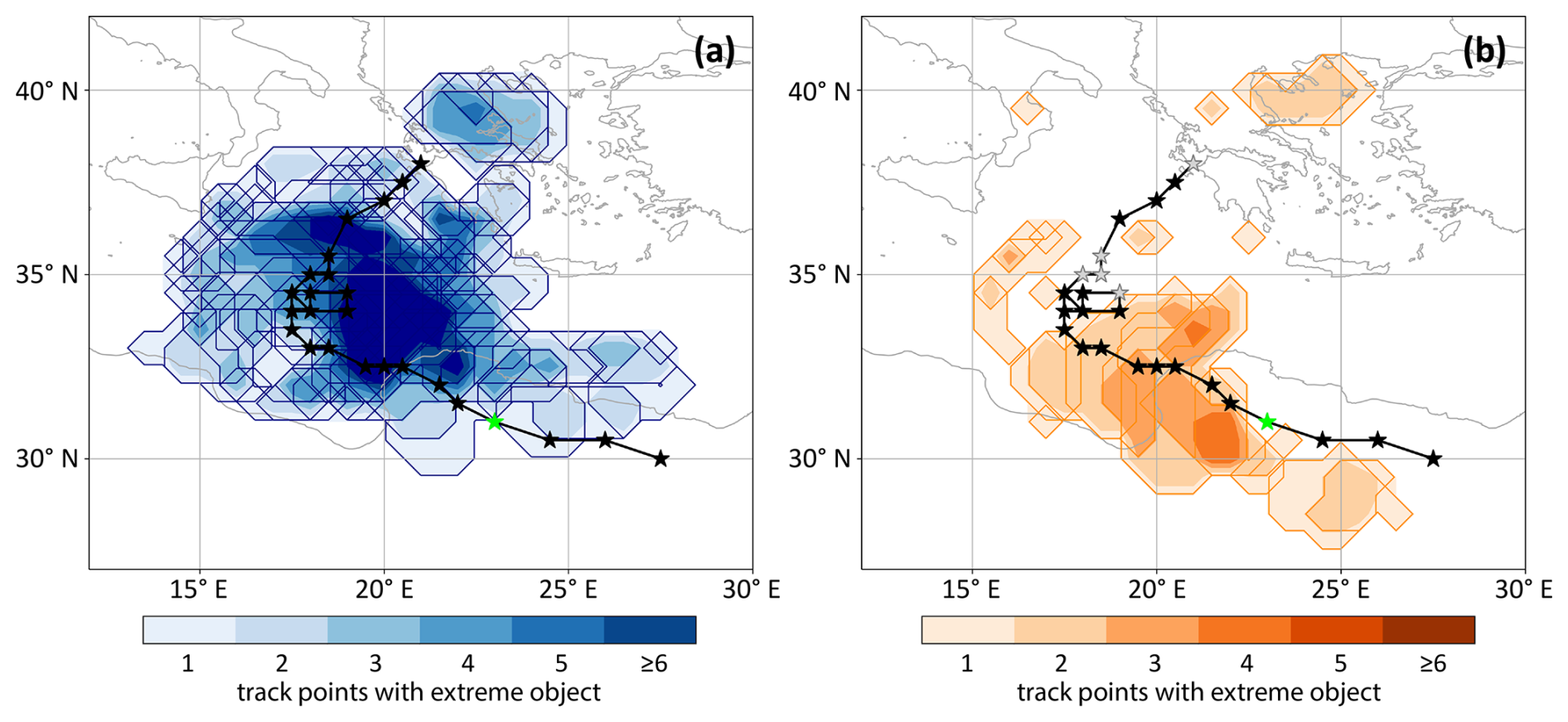
Figure 7 Same as Fig. 3 but for Storm Daniel.

As shown in Fig. 8, Storm Daniel is initially related to a PV streamer stretching from the Ukraine to Italy (Fig. 8a). As discussed in Flaounas et al. (2025), this streamer resulted from an anticyclonic Rossby wave breaking on the eastern flank of an omega-blocking pattern over central Europe. Both the position and orientation of the PV streamer are similar to the PV streamer present in the early phase of Medicane Zorbas in September 2018 (Portmann et al., 2020, their Fig. 2a). During the following days, the PV streamer breaks up and a PV cutoff remains relatively stationary over the sea, which is likely linked to a stationary blocking upstream over Central Europe and in agreement with the slow propagation of the surface cyclone until 10 September (Fig. 8c). The θ-field at 850 hPa (Fig. 8b, d) shows fairly homogeneous values in the region of the cyclone and very high values over northern Africa. During the first intensification stage, P extremes occur northeast and south of the cyclone center at the edge of the PV streamer (Fig. 8a, b), while extreme G₁₀ appears only at single grid points. During re-intensification on 10 September, an area of extreme P is shown northwest of the cyclone center, this time accompanied by extreme G₁₀ west of the cyclone center with both objects overlapping with the upper-level PV cutoff (Fig. 8c).

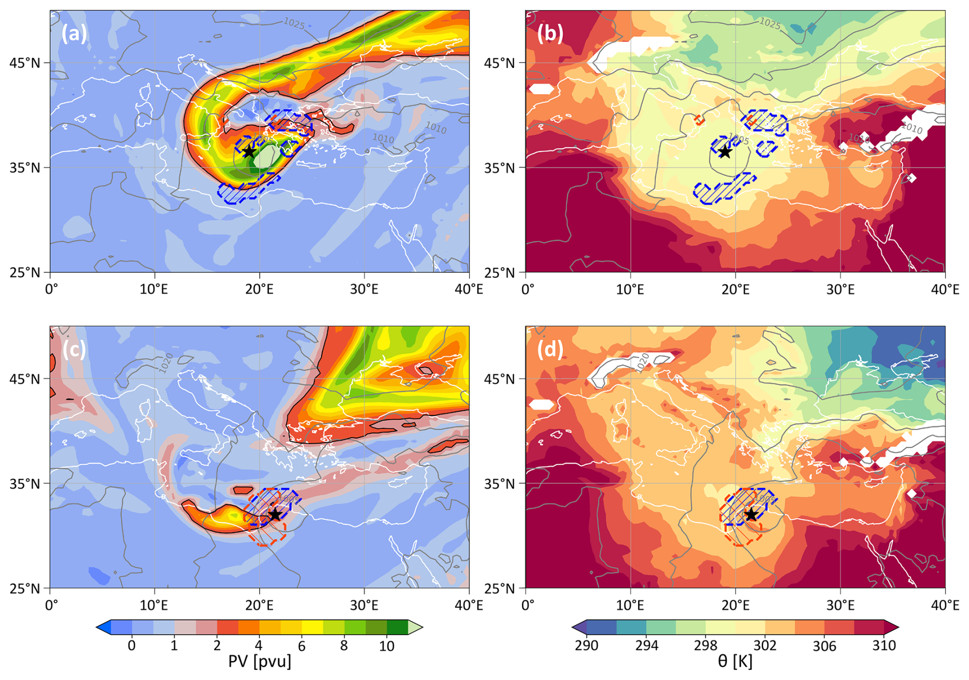
Figure 8 Same as Fig. 4 but for Storm Daniel at (a, b) 12:00 UTC on 5 September (24 h after genesis) and (c, d) 12:00 UTC on 10 September (time of minimum SLP, 144 h after genesis). PV maps show PV at 335 K.

4 ECMWF forecast performance

In the following, we assess the performance of ENS in forecasting the cyclone tracks (Sect. 4.1) and the attributed objects of extreme surface weather (Sect. 4.2) depending on the forecast lead time for the three case studies.

4.1 Cyclone track probabilities

Figure 9 shows the probability of a matching cyclone track in ENS, as a function of time relative to cyclogenesis in ERA5, for all three case studies. This diagram requires careful explanation. Every bar corresponds to an ENS forecast, and for instance a bar labeled at the bottom with “−120” represents a forecast initialized 5 d prior to the time of cyclogenesis in ERA5. The height of the bar indicates the percentage of ensemble members that predict a matching cyclone and therefore cyclogenesis, while the colors denote the predicted time of cyclogenesis relative to the actual cyclogenesis time in ERA5. Yellow and red colors signalize too early cyclogenesis in the ENS members (red colors by 12 to 36 h, see the horizontal bars at the bottom of each diagram) and similarly blue, grey and white colors signalize too late cyclogenesis. Green colors denote the (almost) correct forecast of cyclogenesis time (±6 h). The light blue bar represents the seasonal climatological cyclone frequency in the Mediterranean and is thus an indicator if the forecast data shows a relevant signal or can be regarded as “noise”.

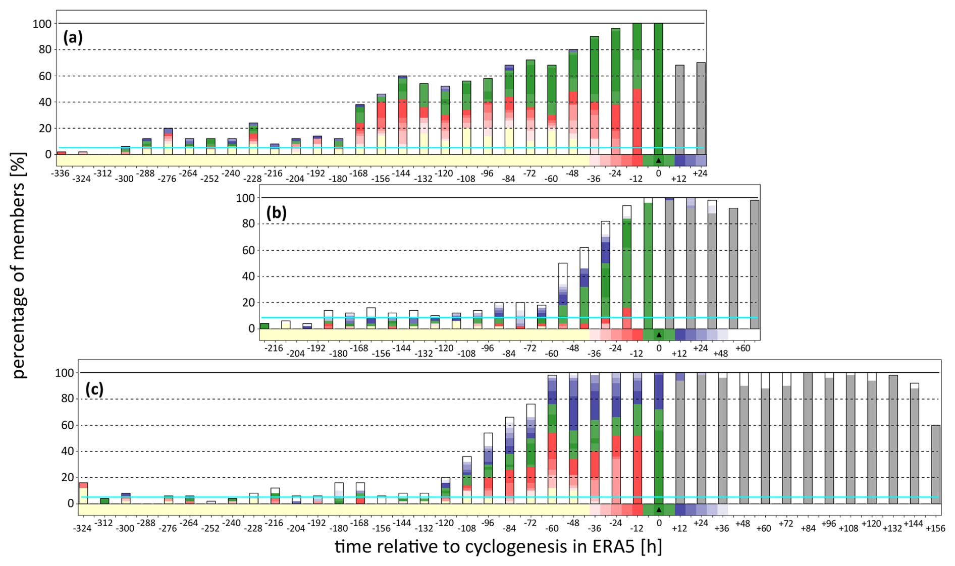
Figure 9 Percentage of members with matching cyclone track (along y axis; in percent) in ENS for Storms (a) Denise, (b) Jan, and (c) Daniel for different lead times (along x axis; in h). Time zero is the time of cyclogenesis in ERA5 (black triangle). Color shading refers to the timing of cyclogenesis in the ENS members (see horizontal bar at the bottom of each panel). Yellow and red colors indicate too early cyclogenesis, blue and white colors too late cyclogenesis, and green an (almost) correct forecast of cyclogenesis time. Grey colors denote members that already have the cyclone at forecast initialization time. Black solid lines denote probability of 100 %. Light blue line denotes an averaged seasonal cyclone frequency as detailed in Sect. 2.3.

Let's consider an example for the first case in Fig. 9a: for the forecast initialized 120 h prior to the time of cyclogenesis in ERA5, about 50 % of the ensemble members produce a matching cyclone track and therefore predict genesis of this cyclone. The bar is colored about half green and half yellow-red, which indicates that half of the members that predict cyclogenesis do this at the correct time (i.e., at day 5 of the forecast, green), whereas the other half produces cyclogenesis too early, in some cases by 2 d or more (yellow). Only very few members produce cyclogenesis too late (blue). In contrast, the forecast initialized only 12 h prior to genesis in ERA5 has a vertical bar that extends to 100 % and the bar is half green and half red. This indicates that in this forecast all members produce the cyclone, half of them at the right time (±6 h, green), and the other half 12 h too early (red).

Already a brief visual comparison of the diagrams for the three cases reveals clear differences in terms of how early most of the ensemble members predicted the cyclone and whether cyclogenesis, if predicted, occurred rather too early or too late. The three cases are discussed in more detail in the following subsections.

4.1.1 Storm Denise

Storm Denise first occurs in ENS 14 d prior to its formation (Fig. 9a). While the probability of cyclogenesis varies between ∼ 10 %–20 % for lead times between 14 and 7 d, a clear increase in probability occurs at −168 with 40 % of all members simulating Storm Denise. While around 60 % of all members predict cyclogenesis for lead times between 144 and 96 h, this probability increases further towards shorter lead times, with about half of the members starting to (almost) correctly forecast the cyclogenesis time (green colors). In the forecast initialized 12 h prior to cyclogenesis, all members predict Storm Denise. Interestingly, only 70 % of the members include the storm in the forecasts initialized at +12 and +24 h, when Storm Denise already exists in the ERA5 dataset. A likely reason for this is the fact that Storm Denise was short-lived (42 h, see Table 1) and that at least 3 time steps are required to fulfill the spatial proximity criterion (Sect. 2.3). Therefore tracks in the ensemble members that are (slightly) too short, may not fulfill this condition.

4.1.2 Storm Jan

Storm Jan first appears in the forecast about 9 d prior to the time of cyclogenesis in ERA5, and thus had a shorter forecast horizon than Storm Denise (Fig. 9b). However, the probability stays below or around 20 % until 66 h prior to cyclogenesis. Only at a lead time of 54 h, an increase in probability up to almost 50 % occurs. In the later forecasts, the probability increases steadily until reaching 100 % 6 h prior to cyclogenesis as well as 6 and 18 h post cyclogenesis. It is noticeable, that at 54, 42 and 30 h prior to cyclogenesis several members predict the onset of the cyclone too late (blue and white colors), and this also holds for the few members that captured the cyclone at longer lead times. As soon as the cyclone exists in ERA5, the probability remains high (between 90 % and 100 %).

4.1.3 Storm Daniel

Storm Daniel occurs in ENS for the first time 13.5 d prior to its genesis; however, until 5 d prior to the time of genesis, less than 20 % of all members forecast the storm (Fig. 9c). A steady increase in probability to 100 % is shown between 120 to 60 h prior to cyclogenesis. After cyclogenesis in ERA5, the forecast probability stays close to 100 % until about 132 h post cyclogenesis, enabled by the longevity of Storm Daniel (see Table 1). Again, it is remarkable that most members miss the actual genesis time of the storm with almost 50 % of all members predicting its genesis too early (red colors at −24 and −12 h) and about 30 %–40  % too late (blue colors).

4.2 Probability of attributed extreme surface weather

As a next and final step, we assess the performance of ENS in predicting the occurrence of extreme surface weather related to the three Mediterranean cyclones. To this end, objects of extreme P and G₁₀ are calculated for each ensemble member as in ERA5 (see Sect. 2.4). Figures 10a, b, 11a, b, and 12a, b show cyclone-centered probabilities of the occurrence of extreme P and G₁₀, as introduced conceptually in Sect. 2.6 and Fig. 2, for the three case studies for different lead times and at different times of the cyclone lifecycle. From here on, these spatial probability fields are referred to as local probability p_loc, whereby a higher value of p_loc at a certain grid point represents a higher number of ensemble members predicting extreme objects at this grid point. Again, these figures are rather involved and require some general introduction. Each panel represents a specific time of the cyclone lifecycle, t_cyc (cyclogenesis corresponds to t_cyc = 0 h), and a specific forecast lead time, t_fc. The panels are arranged in arrays such that forecast lead time decreases from left to right, and time along the cyclone lifecycle increases from bottom to top. As a consequence of this arrangement, panels that belong to the same ENS forecast occur along diagonals (indicated by red dashed lines). Given the long lifetime of some of the cyclones and the many possible forecast lead times, only a selection of panels is shown in the figures. The main aim of these arrays of panels is to illustrate how the probability of correctly predicting extreme objects attributed to the cyclones varies with lead time, during different stages of the cyclones' lifecycle, and between extremes of precipitation and surface wind gusts. Additionally, Figs. 10c, d, 11c, d, and 12c, d show the probability of extreme objects in ENS averaged within the ERA5 object (p_obj; averaged over orange and black contour in panels (a) and (b) above) at different times along the cyclone lifecycle, to further condense the information shown in the panels above. The greater p_obj at a certain timestep t_cyc, the better the prediction of the associated extreme object.

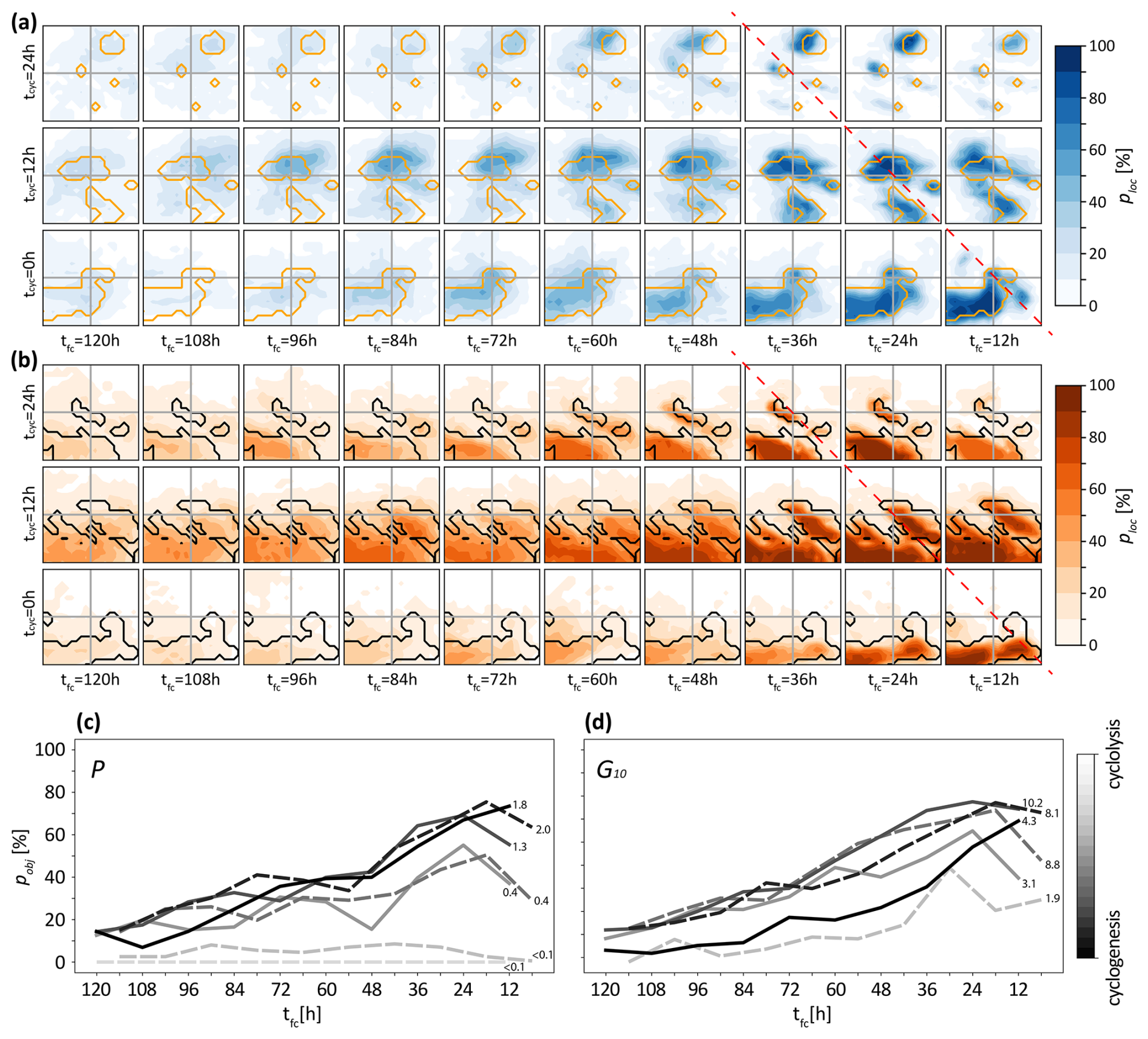
Figure 10 (a, b) Cyclone-centered probabilities (p_loc) of extreme objects of (a) P (blue shading) and (b) G₁₀ (orange shading) during Storm Denise in ENS (in (%)). The orange line in panel (a) and black line in panel (b) denote the extreme P and G₁₀ objects in ERA5, respectively. Lead time decreases along the x axis (t_fc; panels every 12 h) and time along the ERA5 cyclone lifecycle increases along the y axis (t_cyc; with cyclogenesis at t_cyc = 0 h). Composites from the same ENS forecast are positioned diagonally as illustrated by the red dashed line. (c, d) Average probability (p_obj) of extreme (c) P and (d) G₁₀ within ERA5 objects (see Sect. 4.2) as a function of forecast lead time. Each line denotes a separate time along the cyclone lifecycle from cyclogenesis (black line) to cyclolysis (light grey line) in the ERA5 dataset. Solid lines represent time steps shown in panels (a) and (b), other time steps are shown as dashed lines. The area size of the ERA5 object is indicated for each time step as a multiple of 10⁵ km² next to the lines. In panels (c) and (d) cyclone time steps are shown every 6 h for time steps with identified extreme objects in ERA5.

Figure 11 Similar to Fig. 10 but for Storm Jan. Compared to Figs. 10 and 12, the values for t_fc in panels (a) and (b) are shifted by 6 h since the cyclogenesis of Storm Jan happened at 18:00 UTC and, thus, forecasts are available for lead times of 6, 18, and 30 h, etc.

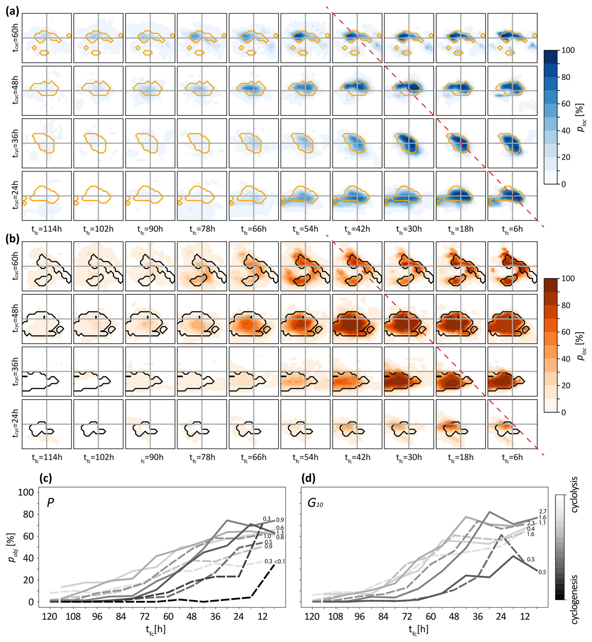
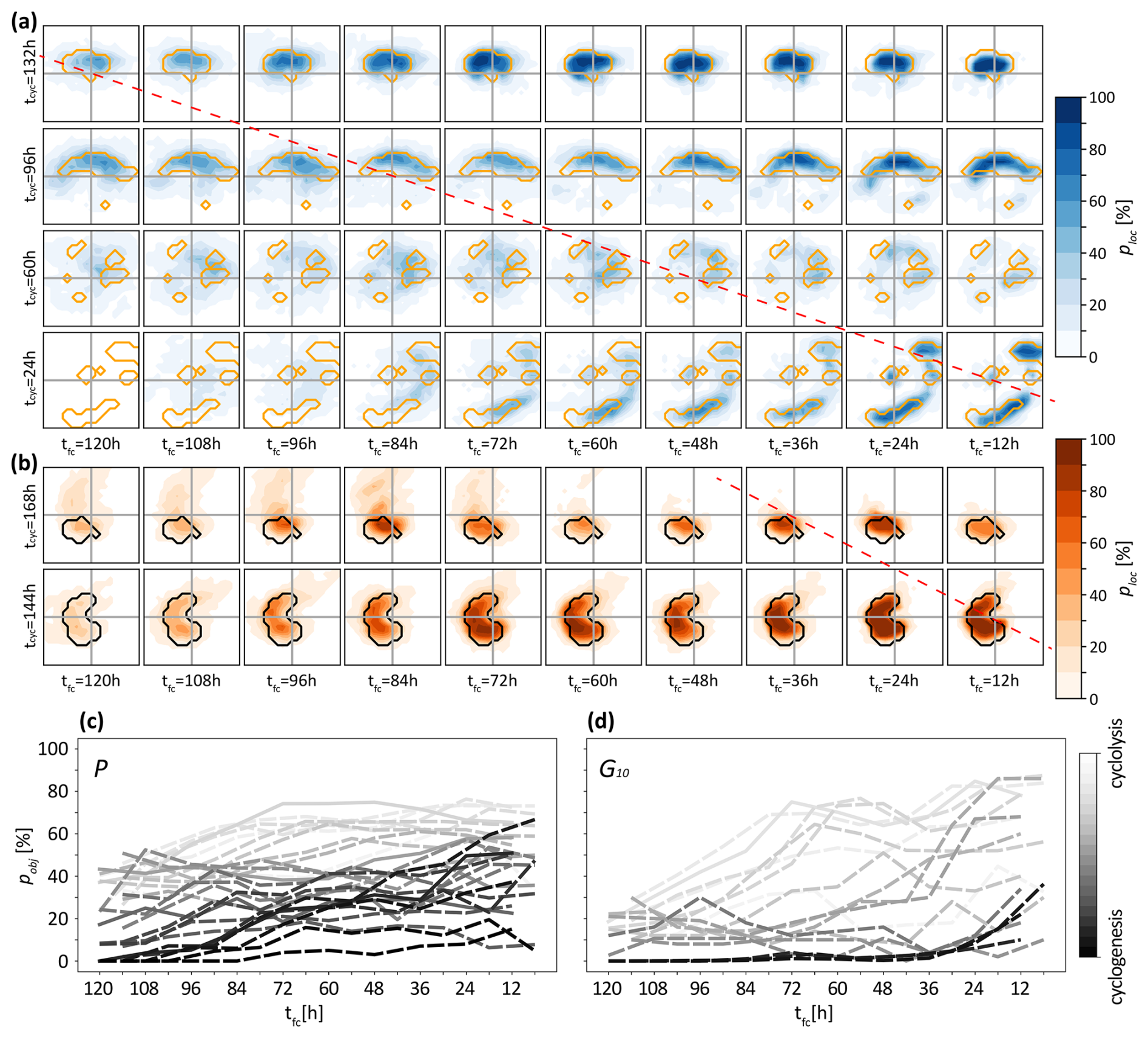
Figure 12 Similar to Fig. 10 but for Storm Daniel. Note that different time steps along the cyclone life cycle are shown for objects of P and G₁₀.

4.2.1 Storm Denise

For Storm Denise, objects of extreme P and G₁₀ have been predicted since the first appearance of the storm in the forecast 336 h prior to the time of cyclogenesis in ERA5 (Fig. 9a). Note, that probability values at the beginning of this time range might still occur within the climatological range. In Fig. 10 we focus on lead times of 5 d and shorter, and the times of genesis (t_cyc = 0 h), minimum SLP (t_cyc = 12 h), and a time during the decay of the cyclone (t_cyc = 24 h). As expected, there is an overall increase in the probability of extreme objects with decreasing forecast lead time, however, with interesting differences at distinct time steps along the cyclone lifecycle (Fig. 10). Relatively large objects of extreme P at t_cyc = 0 h are well forecasted, reaching a p_obj of over 70 % at short lead times (Fig. 10a and black lines in Fig. 10c). At the time of minimum SLP (t_cyc = 12 h), both p_loc and p_obj increase already for longer lead times (dark grey line in Fig. 10c). For later time steps of the storm, a relatively large positional error is shown for the comparatively small P objects, leading to a smaller value of p_obj, which does not exceed 50 % (grey lines in Fig. 10c). Overall, it is notable that for lead times of 5 d or longer some members predict the occurrence of extreme P objects, but their position hardly matches the correct location relative to the cyclone center (see relatively uniform low values of p_loc in the left panels of Fig. 10a).

For wind extremes, a slightly more steady increase in averaged forecast probability is shown in Fig. 10b, d, whereby again the probability at t_cyc = 12 h (maximum intensity; solid dark grey line) is comparatively high at earlier lead times compared to other time steps within the cyclones' life cycle. Similar to precipitation objects, time steps with smaller objects show reduced probabilities, i.e., more uncertain predictions, revealing difficulties of ENS in simulating such small extreme objects at the right place and time.

4.2.2 Storm Jan

As opposed to Storm Denise, objects of extreme P and G₁₀ during Storm Jan are poorly predicted for lead times larger than 54 h, particularly for the early stages of the cyclone life cycle (Fig. 11). Distinct jumps in forecast performance occur at lead times between 54 and 30 h for the first stage of the cyclone for both P and G₁₀ objects (black lines in Fig. 11c, d, t_cyc = 0 h and t_cyc = 12 h in Fig. 11a, b). These jumps occur earlier for the later cyclone stage with a significant increase in object probability for lead times between 66 and 42 h, reaching values of p_obj at or slightly below 80 % at a lead time of about 54 h (grey lines in Fig. 11c, d, t_cyc = 24 h and t_cyc = 36 h in Fig. 11a, b). In comparison with Storm Denise, the positional error of the objects is smaller and areas with a high p_loc match well with the ERA5 objects.

4.2.3 Storm Daniel

Figure 12 shows cyclone-centered object probabilities for Storm Daniel. Incoherent objects of extreme P in the early stage of the cyclone are poorly represented in ENS (Fig. 12a, t_cyc = 24 h and t_cyc = 60 h; black lines in Fig. 12c). Thereby it is important to consider that in case of t_cyc = 24 h, only 20 % of all members contain the cyclone for a lead time of 96 h and still only 50 % of all members for a lead time of 72 h (see Fig. 9c). As extreme P objects become more coherent during the later phase of the cyclone lifecycle, for example, at t_cyc = 96 h and t_cyc = 132 h, and the storm is already existing in ENS for shorter lead times, p_obj reaches values up to 40 % for lead times up to 5 d. The shape of these objects is represented well by the forecast with over 80 % of the members capturing large parts of the object in ERA5, e.g., for a lead time of 72 h in case of t_cyc = 132 h.

The extreme G₁₀ objects that occur during the late stage of Storm Daniel are predicted well in advance, reaching a p_obj of around 60 % for a lead time of 4 d (light grey lines in Fig. 12d) with values of p_loc exceeding 80 % (Fig. 12b). It is noticeable that the ensemble slightly overestimates the size of these objects, particularly for t_cyc=168 h. Very small objects of extreme wind gusts in the early stage of the cyclone that only cover few grid points are poorly or not represented in ENS (not shown).

5 Discussion and conclusions

In this study we assess the performance of operational IFS ensemble forecasts (ENS) in predicting the occurrence of Mediterranean cyclones and attributed objects of extreme precipitation (P) and surface wind gusts (G₁₀). For this aim we introduce a method that is based on several pragmatic choices and can be applied quasi-operationally. We argue that such quasi-operational “online” (or “on-the-fly”) object-based methods will become increasingly important in the future, because the rapidly increasing size of ensemble forecast data will make retrospective “offline” analyses of this kind much more difficult and cost-intensive. Our method includes the following steps:

1. Identify matching cyclones between ERA5 and every ENS member based on spatio-temporal criteria.

2. Define two-dimensional objects of extreme surface weather in both ERA5 and ENS members using ERA5 percentiles as thresholds.

3. Attribute cyclones to extreme weather objects, separately in ERA5 and every ENS member, based on overlap criteria.

4. Calculate ensemble mean cyclone-relative probabilities of predicting extreme objects of P and G₁₀ for different forecast lead times and times along the cyclone life cycle.

To illustrate and test this method, we selected three Mediterranean cyclones with different characteristics. The first case, Storm Denise, has a short lifetime of 42 h and occurs on the front side of a pronounced upper-level PV streamer over the Gulf of Genoa. It is the most intense of the three storms in terms of minimum central SLP. The second case, Storm Jan, originates in the North Atlantic and propagates into the Mediterranean along the rearward flank of an upper-level trough. Storm Jan is the fastest moving and intensifying of the three cyclones. Finally, the third case, Storm Daniel, has an exceptionally long lifetime of 174 h. It is associated with a quasi-stationary upper-level PV streamer and later PV cutoff. Storm Daniel caused persistent extreme P in large areas leading to flooding in both Greece and Libya, while Storm Denise had the largest footprint of extreme surface winds. For these three cases, extreme P usually occurs around the storm center, while extreme G₁₀ is mostly located south of the storm center. This pattern is typically expected for extratropical cyclones, while medicanes usually feature extreme winds all around the storm center (e.g., Raveh-Rubin and Wernli, 2016; Miglietta et al., 2025).

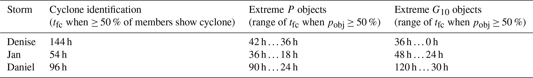
The analysis of the three cyclones in the ENS dataset shows a general increase in probability of both the occurrence of the cyclone track itself and of the attributed extreme surface weather with decreasing forecast lead time. In particular, we find a high forecast probability for extreme objects for lead times ≤ 48 h. For longer lead times, our study reveals a large case-to-case variability in the predictability of both the cyclone track and its attributed extreme surface weather (see also summary in Table 2). While 40 % of the ensemble members predict Storm Denise 7 d prior to its genesis, the same value is reached only 4.5 d prior to genesis of Storm Daniel and only 2.5 d prior to genesis of Storm Jan. These results are consistent with Doiteau et al. (2024) who found that on average more intense storms in terms of minimum SLP (such as Storm Denise) are detected by more ensemble members at longer lead times, and that rapidly-intensifying storms (such as Storm Jan) show a particularly low forecast skill. In the case of Storm Denise, an initial increase in forecast probability of the cyclone track is followed by a stagnant phase between 6 and 4 d prior to cyclogenesis and a gradual increase afterwards. In contrast, Storms Jan and Daniel exhibit a more rapid increase in forecast probability of their tracks. The actual formation of the storms is predicted on average slightly too early for Storms Denise and Daniel, and slightly too late for Storm Jan. It should be noted that differences in the prediction of the cyclogenesis time (red, blue, and green colors in Fig. 9) can be affected by the cyclone's lifetime. The likelihood of predicting the genesis of a shorter-lived cyclone as Storm Denise too late is smaller compared to a long-lived cyclone such as Storm Daniel, since there are fewer possible cyclogenesis time steps that still allow for a cyclone matching based on our matching criteria. Late forecasts initialized after cyclogenesis in ERA5 show a probability of 90 %–100 % for Storms Jan and Daniel, matching findings by Di Muzio et al. (2019) about the higher accuracy of later forecasts that are initialized after cyclogenesis. For Storm Denise, ENS shows a notable reduction in probability to less than 70  % at this stage, which is probably linked to the short lifetime of this storm, which could cause less members fulfilling the spatio-temporal criterion for matching cyclone tracks between ENS and ERA5.

Table 2 Overview of the predictability analysis of Storms Denise, Jan, and Daniel in the ENS dataset showing (first column) the earliest lead time (t_fc) when at least 50 % of the ensemble members detect a matching cyclone, and (second and third column) the range of lead times when p_obj, the probability of extreme P and G₁₀ averaged within the extreme object in ERA5 (see Sect. 4.2), reaches at least 50 %. This lead time can vary along the cyclone life cycle (see Figs. 10–12). Note, that only time steps are considered when the area size of the extreme object in ERA5 is at least 10⁵ km².

The predictability of objects of extreme surface weather exhibits a similarly strong case-to-case variability. For Storm Denise, such objects are already predicted in up to 40 % of all members at a lead time of 120 h, followed by a staggered probability increase at lead times of 72 and 24 h. However, despite the early detection of the objects, a relatively large positional error remains also for short lead times, particularly for extreme P objects. Distinct jumps in object probabilities occur for the forecast of extreme surface weather attributed to Storms Jan and Daniel, which both feature comparatively small positional errors of such objects relative to the storm center.

Although three cases are not enough to draw robust generalized conclusions, our case studies indicate three key aspects that affect the probability of extreme surface weather objects in ENS forecasts:

1. Object size. We find that larger and more coherent objects are usually better represented compared to multiple small objects. This partially follows by design, as we define such objects with a (percentile-based) threshold. For small objects, values of P and G₁₀ are usually close to the threshold value, resulting in a higher ensemble uncertainty of simulating the object.

2. Cyclone track. A better representation of the cyclone in ENS results in an improved predictability of extreme surface weather objects at longer lead times. In case of Storm Denise, which is already simulated by ∼ 50 % of the ensemble members a week prior to its actual formation, the forecast of extreme surface weather objects is less uncertain compared to Storms Jan and Daniel, which are captured by fewer ensemble members at similar lead times. This is illustrated by Fig. S4, which shows conditional probabilities² of the occurrence of surface extreme weather objects as opposed to the probabilities shown in panels (c) and (d) of Figs. 10, 11, and 12. Compared to the other two cases, conditional probabilities are higher for Storm Denise at long lead times, indicating that for this cyclone, members including the storm already have a good representation of the attributed extreme weather compared to members including Storms Jan and Daniel at the same lead times.

3. Storm lifecycle. We reveal an increase in the probability of predicting extreme weather objects with increasing cyclone lifetime for similar lead times, for the cyclone stages with a similar area size of extreme weather objects. This likely is a consequence of the existence of the cyclone in almost all members in forecasts of later storm stages, while forecasts for early storm stages are affected by a significant amount of members not including the storm. In essence, this indicates that for the cases investigated here, the process of cyclogenesis is more uncertain, i.e., more challenging to simulate, than the later cyclone intensification and decay.

Overall, we show that, for the three cyclones investigated, ENS predicts objects of extreme surface weather very well with respect to the storm center for lead times up to about 2 d. For longer lead times, the forecast uncertainty of extremes appears to be strongly case dependent. Although it would be presumptuous to derive climatological conclusions from the investigation of only three storms, the case-to-case variability shown across the three cases already implies challenges in deriving simple general guidelines about extreme weather predictability, for example, for early warning systems. We conclude that the proposed methods can yield meaningful information about the ensemble prediction of surface weather extremes and we plan to apply the method systematically to a multi-year dataset of Mediterranean cyclone forecasts. However, it is also important to mention caveats of this study: (i) we analyze the probability of objects only relative to the cyclone center without investigating the error in the cyclone center position; (ii) we only quantify whether ensemble members exceed a certain threshold, but not by how much (which would be relevant, e.g., for flood prediction in case of extreme P objects); (iii) to facilitate the comparison we compared ERA5 and ENS on a grid with 0.5° horizontal grid spacing and reduced the temporal resolution of the ERA5 cyclone tracks to 6 h, which impedes a more detailed analysis and taking full advantage of the respective dataset resolution. This is especially relevant when looking at small objects of extreme surface weather and due to the fast evolution of storms in the Mediterranean. Furthermore, while ensuring the feasibility of our method, unavoidable limitations of this study include the spatiotemporal resolution of our forecast dataset, the coverage of different operational cycles, as well as pragmatic methodological choices.

As mentioned above, in the second part of this study we plan to apply the method introduced here to a large set of Mediterranean cyclones. This serves to potentially identify differences in forecast performance between cyclones with different characteristics, for instance in terms of their upper-level PV signature at time of maximum intensity (Givon et al., 2024) and of upstream processes over the North Atlantic that might influence the dynamical evolution and forecasts performance over the Mediterranean (Raveh-Rubin and Flaounas, 2017; Portmann et al., 2020; Scherrmann et al., 2024). Such analysis will improve our understanding of the large case-to-case variability found in this study, and potentially of the underlying causes for forecast errors in terms of intensity, location and area size of surface weather extremes. It will further allow us to draw more robust conclusions about societally relevant aspects including the forecast horizon of Mediterranean cyclones and their associated extremes, which are of interest for early warning systems.