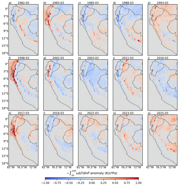
Explaining monthly precipitation anomalies in northwestern South America by integrating vertical dynamics and energetics

In dynamically limited environments such as the coastal Northwestern South America (NWSA), thermodynamic instability (ΔT) alone is insufficient to autonomously trigger deep convection due to persistent background subsidence. The Buoyancy Work Rate (BWR) addresses this boundary constraint by vertically coupling ΔT with vertical velocity (ω). A causal discovery analysis empirically verified this formulation, demonstrating that the BWR preserves the dominant causal route to precipitation over other individual thermodynamic or dynamic variables, successfully capturing the dynamic trigger required to realize convection. As a diagnostic proxy, the BWR systematically outperforms established thermodynamic indices because it explicitly quantifies the realized mesoscale atmospheric response rather than just the precursor potential. This diagnostic advantage is reinforced by an upper tail dependence analysis based on empirical copulas, which confirmed the index's robustness during extreme hydroclimatic anomalies. Moreover, while isolated mid-level vertical velocity dictates instantaneous convection, its high-frequency volatility limits its utility for continuous monitoring. By integrating ΔT, the BWR mathematically inherits the thermal inertia of the oceanic boundary conditions, imparting greater signal persistence and making it a more stable proxy for sub-seasonal operative monitoring. Ultimately, the operational value of the BWR emerges in its prognostic application. By substituting predicted precipitation anomalies from the SEAS5 model with the predicted BWR anomalies, the predictions overcome the limitations of the sub-grid parameterizations inherent in the climate model. Relying instead on explicitly resolved mesoscale variables governed by primitive equations, the BWR systematically improves seasonal predictive skill during the peak of the austral summer and mitigates the forecast degradation caused by the boreal spring predictability barrier.

1 Introduction

It is physically well-established that deep moist convection in the tropical Pacific is primarily governed by large-scale atmospheric dynamics and horizontal moisture convergence, rather than exclusively by local Sea Surface Temperature (SST) (Lau et al., 1997; Bony et al., 1997). The work of Cornejo-Garrido and Stone (1977) demonstrated that, on climatic timescales within the Walker circulation, latent heat release in the atmospheric column is fundamentally balanced by the adiabatic cooling induced by large-scale vertical ascent. This thermodynamic equilibrium dictates that large-scale atmospheric circulation and deep convection are inextricably coupled (Emanuel et al., 1994). Within this framework, time-mean sources of tropospheric column-integrated moist static energy must be balanced by the advective export of energy driven by divergent circulations (Neelin and Held, 1987). Consequently, the atmospheric convective response is dynamically maintained by mass and horizontal moisture convergence (Back and Bretherton, 2005).

This dynamic dominance is highly evident in Northwestern South America (NWSA). The coastal subdomain between Peru and Ecuador is typically characterized by a persistent subsidence (dynamically limited environment) with a short rainy season during the austral summer. However, the disturbance of this regional circulation during strong El Niño events (e.g., 1982–1983, 1997–1998, 2017, and 2023) triggers extreme hydroclimatic anomalies, causing severe flooding and socio-economic impacts (Bendix, 2000; Takahashi, 2004; Callahan and Mankin, 2023; Poveda et al., 2025). Notably, not all warming events manifest similarly: the 2015–2016 global El Niño recorded historically high SSTs but failed to produce comparable extreme hydroclimatic anomalies along the NWSA coast (Paek et al., 2017). This paradox is explained by the region's physical constraints. Although local SST must exceed a specific threshold to trigger atmospheric instability (Woodman, 1999; Takahashi, 2004; Jauregui and Takahashi, 2018), this atmospheric instability (ΔT) is a necessary but insufficient condition for deep convection (Williams and Renno, 1993). Once the thermodynamic threshold is surpassed, control shifts predominantly to the large-scale vertical velocity (ω) (Lau et al., 1997; Bony et al., 1997). Convection often requires a mechanical trigger, such as the localized vertical ascent generated by the sea breeze colliding against the western Andean slope (Takahashi, 2004; Rollenbeck et al., 2022), which lifts air parcels to their Level of Free Convection (LFC) to initiate latent heat release. The ensuing mid-level ω emerges to balance this diabatic heating through adiabatic cooling (Sobel et al., 2001), stimulating further low-level horizontal convergence dictated by mass continuity (Back and Bretherton, 2005).

Despite this established dynamic-thermodynamic coupling, the operational assessment of precipitation has traditionally based on purely thermodynamic stability indices. E.g., the Convective Available Potential Energy (CAPE) (Emanuel et al., 1994), which evaluates the integrated atmospheric instability for an ascending air parcel from the Level of Free Convection (LFC) to the Equilibrium Level (EL). Or the Gálvez-Davison Index (GDI) (Gálvez and Davison, 2016), which represents better tropical environments, incorporating low-to-mid tropospheric moisture availability and the stabilizing effects of trade-wind inversions. However, the GDI does not necessarily relate to regions of dynamically induced ascent or descent (WPC, 2022). In environments with persistent subsidence like the coastal subdomain, relying exclusively on thermodynamic metrics yields high false-positive rates because they cannot distinguish between active deep convection and dynamically suppressed atmospheric instability (DeMott and Randall, 2004). To overcome this limitation, the Buoyancy Work Rate (BWR) is proposed as a diagnostic proxy. By mathematically coupling the atmospheric instability (ΔT) directly with the vertical velocity (ω), the BWR inherently incorporates the kinematic realization of convection, diagnosing active convective engines while filtering out thermodynamically unstable but dynamically suppressed environments.

The objective of this study is to evaluate the diagnostic capability, physical interpretation, and prognostic utility of the BWR index for extreme hydroclimatic anomalies in the NWSA. First, the PCMCI+ data-driven causal discovery algorithm (Runge, 2020) is used to empirically evaluate the preservation of the BWR causal route to precipitation. Second, the reliability of the BWR during extreme hydroclimatic anomalies is assessed using the Upper Tail Dependence coefficient derived from empirical copulas (Nelsen, 2006; Poulin et al., 2007). Third, an autocorrelation analysis demonstrates how the inclusion of the atmospheric instability component imparts greater signal persistence to the index compared to pure vertical velocity. Finally, to evaluate its true prognostic utility, the operational prediction skill of the BWR is explicitly tested by applying the index to predicted atmospheric fields from the ECMWF SEAS5 model, assessing whether this physical translator systematically outperforms the model's direct precipitation predictions for early warning applications.

2 Data and study area

2.1 Observational, Reanalysis, and Forecast Data

Monthly mean air temperature (T_a), relative humidity (RH), and zonal, meridional, and vertical wind components were obtained from the ERA5 reanalysis dataset (Hersbach et al., 2020). These data were utilized for the period 1981–2025 across 27 vertical pressure levels ranging from 1000 to 100 hPa, with a spatial resolution of 0.25°. Monthly SST from ERA5 was also utilized to provide context for the identified extreme hydroclimatic events. The SST data from the ERA5 reanalysis – which strictly prescribes observation-based products such as HadISST2 and OSTIA (Hersbach et al., 2020) – were used to characterize the oceanic boundary conditions. The use of ERA5 SST, rather than an independent observational product, ensures strict thermodynamic consistency, as it represents the exact surface forcing that generated the atmospheric response (ω and ΔT) evaluated in this study.

To validate the proposed climate index, two independent high-resolution precipitation products developed specifically for the complex Peruvian topography were employed. First, the RAIN4PE product (Fernandez-Palomino et al., 2022) was used for the 1981–2015 period. RAIN4PE is a gridded dataset that merges three data sources – satellite estimates (CHIRPS), reanalysis data (ERA5), and ground observations – corrected via quantile mapping and validated through hydrological modeling to ensure consistency with observed streamflow and water balance closure. Second, the PISCO product (Peruvian Interpolated Data of the SENAMHI's Climatological and Hydrological Observations) (Aybar et al., 2019) was used for the 1981–2025 period. PISCO is a hybrid product developed by the National Meteorology and Hydrology Service of Peru (SENAMHI) that combines quality-controlled rain gauge records with satellite covariates (CHIRPS) using geostatistical interpolation techniques to reconstruct rainfall fields over data-scarce regions. It is important to note that the stable version of PISCO, which incorporates both manual and automatic quality control (Aybar et al., 2019), is available only for the 1981–2016 period; consequently, the unstable version, which undergoes only automatic quality control, was utilized for the 2017–2025 period.

Monthly precipitation from ERA5 (Hersbach et al., 2020) was used to identify the area within the NWSA exhibiting the highest similarity with observational datasets, given that the proposed index is constructed entirely from ERA5 variables. Figure 1 shows that ERA5 is significantly correlated with RAIN4PE and PISCO over the entire domain, being strongest near the coast between Peru and Ecuador. This high correlation along the coastal strip is primarily due to large-scale synoptic and dynamic boundaries that global reanalyses effectively resolve, coupled with a high density of meteorological stations that enhances the reliability of PISCO and RAIN4PE in this specific subregion (Aybar et al., 2019; Fernandez-Palomino et al., 2022).

Conversely, the correlation weakens significantly over the Andes and the Amazon basin. Over the Andes, ERA5’s spatial resolution is too coarse to adequately capture fine-scale orographic precipitation, systematically leading to overestimations (Insel et al., 2009; Fernandez-Palomino et al., 2022). In contrast, regional gridded products mitigate this by incorporating local terrain elevation models and dense gauge networks. Over the Amazon basin, precipitation is largely driven by localized mesoscale convective systems and intense moisture recycling (Poveda et al., 2006), which remain challenging for ERA5's convective parameterizations to simulate accurately. This physical discrepancy is further compounded by the sparse distribution of rain gauges in the Amazon, which sharply increases the spatial interpolation uncertainty in observation-based datasets (Sun et al., 2018; Fernandez-Palomino et al., 2022).

Furthermore, to evaluate the prognostic utility of the BWR index, predicted atmospheric variables and direct precipitation outputs were obtained from the fifth generation of the ECMWF seasonal forecasting system (SEAS5) (Johnson et al., 2019). SEAS5 is an operational coupled global climate model designed for long-range predictions. Given the inherent uncertainty and chaotic nature of seasonal forecasting, this study specifically utilizes the monthly ensemble means of the real-time forecasts rather than individual deterministic members. This approach filters out high-frequency internal variability, isolating the predictable macro-scale signal required for the BWR calculation. The forecast data spans the operational period from 2017 to 2025.

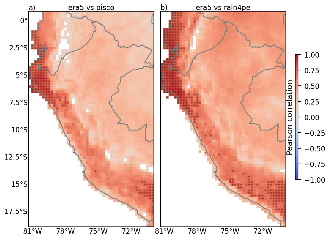
Figure 1 Pearson correlation (R) at the 95 % confidence level between monthly precipitation anomaly from ERA5 and PISCO (a) for 1981–2025, and RAIN4PE (b) for 1981–2015. Only pixels with significant R (p-value <0.05) are shown, the gray points represent R>0.7. The blue (red) shaded colors indicate negative (positive) values of R. Anomalies were calculated taking the 1981–2015 median as climatology for all datasets.

2.2 Study area: The NWSA and the coastal coupling zone

Two domains of interest were defined: the broader NWSA region (81.6–67.05° W, 18.95° S–1.5° N) and a specific coastal subdomain adjacent to the Niño 1+2 region (81.25–78.5° W, 8° S–0.75° N) (Fig. 2).

The coastal subdomain NWSA (Fig. 2b) is typically located under the regional branch of the Walker circulation, characterized by persistent subsidence and trade-wind-driven coastal upwelling that suppresses convection. This stability is reinforced by the mid-level easterly flows, which, upon crossing the Andes, descend, forcing a dry leeward subsidence on the coastal strip (Quispe, 2018; Rollenbeck et al., 2022), but this subsidence weakens during the short austral summer. However during El Niño events, this subsidence regime collapses: the South Pacific Anticyclone migrates southward, upwelling weakens, and warm sea surface temperatures (SST) invert the low-to-mid-level flows into anomalous westerlies below 5 km (Douglas et al., 2009), generated by the sea breeze colliding against the western Andean slope (Takahashi, 2004; Rollenbeck et al., 2022). This westerly moisture advection around 600 hPa becomes essential to organize convective systems and couple them with the second band of the ITCZ (Aliaga-Nestares et al., 2023; Rivas Quispe et al., 2024), while low-level sea breezes force windward orographic ascent that helps air parcels reach their level of free convection (Horel and Cornejo-Garrido, 1986; Goldberg et al., 1987; Bendix and Bendix, 1998; Takahashi, 2004). Physically, this dynamically limited region operates as a thermodynamic switch governed by Strict Quasi-Equilibrium (SQE) dynamics: during dry months, the SQE is decoupled and net vertical motion (ω) fluctuates without producing rain; but once the SST exceeds the critical ∼26 °C threshold (Woodman, 1999; Takahashi and Dewitte, 2016; Jauregui and Takahashi, 2018), the inversion breaks and the system enters a rigidly coupled SQE regime, where ω and the latent heat of precipitation feed each other in a contemporaneous, bidirectional loop (Cornejo-Garrido and Stone, 1977; Emanuel et al., 1994).

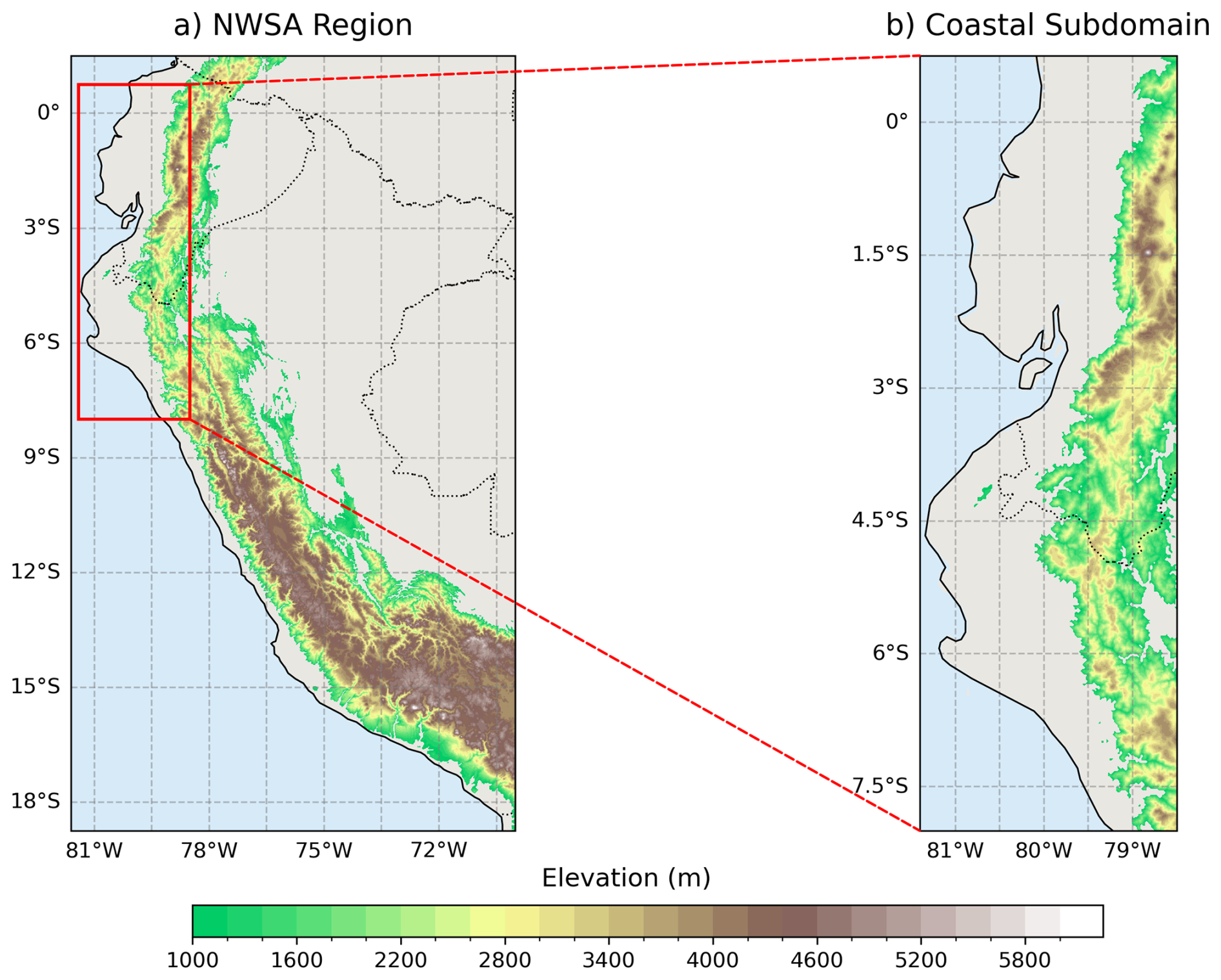
Figure 2 Study domains: the broader NWSA region (a) (81.6–67.05° W, 18.95° S–1.5° N) and the coastal subdomain (b) (81.25–78.5° W, 8° S–0.75° N).

Figure 3 presents the precipitation climatology (1981–2025) from PISCO averaged over this coastal subdomain. It is observed that March constitutes the rainiest month; this seasonal peak represents a critical coupling window when dynamic relaxation (weakening of trade winds) and atmospheric instability (SST warming) come into phase, facilitating the development of deep convection (Takahashi, 2004; Poveda et al., 2006; Adachi et al., 2018; Peng et al., 2024).

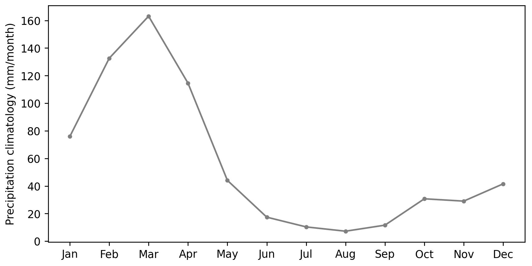
Figure 3 Precipitation climatology as the 1981–2025 mean from PISCO averaged over the coastal subdomain.

3 Methodology

3.1 Identification of extreme hydroclimatic anomalies as Diagnostic Case Studies

To characterize the distinct vertical atmospheric configurations associated with extreme hydroclimatic anomalies, a set of representative case studies was identified. Monthly precipitation was averaged over the coastal NWSA subdomain (Fig. 2b), and anomalies were calculated from the PISCO dataset relative to the 1981–2015 climatological mean. Two thresholds, corresponding to the 5th and 95th percentiles, were defined solely for event selection purposes: anomalies below 5th percentile were used to detect significant dry events, and anomalies above 95th percentile were used to detect extreme rainy events. It is important to clarify that these thresholds were applied exclusively to select events for physical diagnosis (e.g., analyzing vertical structure) and were not utilized to calibrate or derive the formulation of the proposed index. To determine the spatial core of these anomalies, the vertical motion field was analyzed through latitudinal and longitudinal cross-sections (see Figs. 10 and 9 in Sect. 4). The longitude of 80° W and latitude of 5° S were identified, approximately, as the axes of maximum vertical ascent over the coastal subdomain. This geometric characterization allowed for the identification of subsidence and convective layers, as well as the specific pressure levels where convection was initiated and suppressed during the selected case studies.

3.2 Buoyancy Work Rate (BWR) formulation

The formulation of the BWR is physically grounded in the thermodynamic energy balance of the Walker circulation described by Cornejo-Garrido and Stone (1977), which posits that on climatic timescales, latent heat release is primarily balanced by adiabatic cooling due to vertical motion. Consequently, an index capable of explaining precipitation anomalies in this region must explicitly couple the atmospheric instability with the dynamic forcing (vertical velocity) required to overcome the persistent background subsidence.

First, the dew point temperature (T_d) was calculated from relative humidity following Bolton (1980). Using surface T_d and air temperature (T_a), the parcel temperature path was computed and compared against the environmental temperature profile to yield the parcel buoyancy (ΔT) for every grid point. To construct the index, the product of vertical velocity (ω) and parcel buoyancy (ΔT) was analyzed. The Buoyancy Work Rate (BWR) is defined as the vertical integration of this product from the surface to 100 hPa with respect to the natural logarithm of pressure (dln P), as shown in Eq. (1).

$$\begin{array}{}\text{(1)}& \mathrm{BWR}=-\underset{\mathrm{sfc}}{\overset{\mathrm{100}}{\int }}\mathit{\omega }\mathrm{\Delta }Td\ln P\end{array}$$

In this integration, only layers exhibiting positive buoyancy (ΔT>0) and upward motion (ω<0) were included. This constraint ensures that the index specifically quantifies the rate at which potential energy is converted into kinetic energy during deep convection, filtering out stratiform or forced ascent in stable environments.

To understand this diagnostic formulation, it is instructive to mathematically and conceptually contrast the BWR with CAPE. CAPE is defined as the vertical integral of parcel buoyancy from the level of free convection to the equilibrium level (Emanuel, 1994). It strictly evaluates the precursor thermodynamic potential energy available for convection, remaining mathematically blind to whether a dynamic trigger actually exists to overcome background subsidence (Fu et al., 1999; DeMott and Randall, 2004). In contrast, the BWR is formulated by integrating the product of thermodynamic instability (ΔT) and vertical velocity (ω) across the atmospheric column. Rather than measuring stored static potential, this hybrid formulation explicitly quantifies the realized rate of kinetic energy conversion. By mathematically coupling buoyancy with mesoscale kinematic ascent, the BWR imposes a strict physical constraint: it systematically penalizes and zeroes out environments that possess massive thermodynamic instability (high CAPE) but remain mechanically suppressed by persistent subsidence (ω>0).

3.3 Validation framework

To evaluate the physical robustness and predictive utility of the BWR, a multi-tiered validation framework was implemented, moving from causal verification to statistical comparative evaluation.

3.3.1 Causal discovery and physical drivers

To causally evaluate the proposed Buoyancy Work Rate (BWR) index and its diagnostic validity for precipitation anomalies in the coastal NWSA, a causal discovery analysis was conducted using monthly time series for the 1981–2025 period. The PCMCI+ algorithm (Runge, 2020) was applied to navigate this framework. Unlike its predecessor, PCMCI+ is specifically designed to discover both time-lagged and contemporaneous (lag−0) causal relationships in highly autocorrelated time series. This capability is fundamentally required for this study, as the macro-scale dynamic and thermodynamic interactions governing precipitation at monthly timescales occur predominantly at lag−0.

The methodology operates through two core phases. First, a lagged condition-selection step (based on the PC algorithm) is executed to iteratively estimate the lagged parents of each variable. This step filters out spurious autocorrelations and drastically reduces the dimensionality of the conditioning sets. Second, the algorithm applies the Momentary Conditional Independence (MCI) test to evaluate the remaining lagged and contemporaneous links. Crucially, the MCI test evaluates the conditional independence between two variables by simultaneously conditioning on the estimated past of both variables. By explicitly optimizing these conditioning sets, the MCI test isolates the true causal signal from the inherent background noise induced by strong autocorrelation, yielding a highly calibrated estimate of the partial correlation (causal strength).

The causal analysis was performed using time series of monthly standardized anomalies, and the statistical robustness of the inferred causal links was evaluated using a bagging bootstrapping procedure with 3000 samples. To accurately represent the land-atmosphere interaction, precipitation was averaged strictly over the land pixels of the coastal NWSA subdomain. In contrast, local evaporation, vertical velocity at 500 hPa (ω₅₀₀), and parcel buoyancy (ΔT_700−400) as atmospheric instability proxy were averaged over the entire coastal NWSA bounding box (incorporating ∼21 % oceanic area) to capture the regional atmospheric boundaries. SST averaged over the Niño 1+2 region was set as an exogenous boundary condition. To facilitate the physical interpretation of the causal links, the signs of vertical velocity and evaporation were inverted (−ω₅₀₀ and −E, respectively) prior to input, ensuring that positive values strictly indicate upward mass and upward moisture fluxes. The 500 hPa level was specifically selected because it typically corresponds to the level of maximum vertical mass flux in the tropical troposphere, ω at this mid-tropospheric level serves as the most robust proxy for the column-integrated adiabatic cooling required to balance convective latent heat release.

In our reference causal network (Fig. 7a), we utilize the PCMCI+ algorithm restricted to contemporaneous relationships (Runge, 2020). The relationship between atmospheric dynamics and precipitation is dominated by a simultaneous circularity known as the convergence feedback (Back and Bretherton, 2005). Because a purely contemporaneous algorithmic configuration cannot resolve the temporal sequence to isolate the portion of the variance where large-scale dynamics perturbed the environment prior to the onset of deep convection (Fu et al., 1999), we explicitly break this statistical circularity by imposing directional physical link assumptions. By doing so, we enforce a strict physical hierarchy that imposes the mesoscale dynamics as the boundary condition that authorizes or restricts convection, isolating this mesoscale environmental forcing from local and sub-grid scale convective processes (Lau et al., 1997; Bony et al., 1997). This theoretically grounded causal network serves exclusively as a physical baseline to evaluate whether our proposed BWR index successfully preserves the mesoscale thermodynamic and dynamic signals governing precipitation.

The second causal network was evaluated by introducing the BWR index. It must be clarified that the BWR evaluated in this network is not the simplified product of −ω₅₀₀ and ΔT_700−400, but rather the strict vertical integration defined in Eq. (1). In addition, the mid-level vertical velocity (−ω₅₀₀) and the atmospheric instability (ΔT_700−400) were explicitly removed from the algorithm to prevent deterministic collinearity. It is important to note that our objective with this network is not to discover the drivers of precipitation, as these have been extensively documented by previous works (e.g., Lau et al., 1997; Woodman, 1999; Takahashi, 2004), but rather to assess whether the BWR index acts as a causal driver of precipitation. Because the algorithm was restricted to contemporaneous relationships, we imposed two directional physical link assumptions (from SST to -E, and from SST to BWR). These constraints dictate that while a statistical relationship might not necessarily exist between these variables, if one is detected, it must follow this physically grounded direction. This approach breaks the simultaneous statistical circularity of the system.

3.3.2 Statistical comparative evaluation with established indices

The diagnostic skill of the BWR was compared with established indices previously tested in the region: the Convective Available Potential Energy (CAPE) (Emanuel, 1994) and the Gálvez-Davison Index (GDI) (Gálvez and Davison, 2016), both evaluated for the NWSA by Rivas Quispe et al. (2024); as well as the asymmetric (I_a) and double ITCZ (I_d) indices proposed by Yu and Zhang (2018), assessed by Aliaga-Nestares et al. (2023). However, this comparison must be interpreted under a strict physical distinction. While indices such as CAPE and the GDI solely quantify the thermodynamic potential for convection based on precursor conditions, the BWR is designed to explicitly measure the realized mesoscale atmospheric response. This fundamental asymmetry arises because the BWR incorporates mesoscale vertical velocity (ω), thereby directly capturing the ascending motion physically coupled with precipitation. Bearing this distinction in mind, their diagnostic performance was evaluated using the spatial distribution of the Pearson correlation coefficient (R) between the indices and three precipitation products (ERA5, PISCO, RAIN4PE) for the 1981–2015 period.

Given that the evaluated indices and precipitation products possess disparate physical dimensions and scales, all time series were converted to standardized anomalies strictly for the generation of scatterplots and temporal series to ensure comparable variance visualization. Finally, to evaluate performance specifically over the coastal subdomain, indices and precipitation were averaged over land pixels within the subdomain defined (Fig. 2b). Scatterplots and time series were analyzed to identify regimes where the BWR offers advantages or limitations compared to purely thermodynamic or precipitation-based indices.

3.3.3 Analysis of extremes, signal persistence, and predictive capability

Standard correlation metrics often underestimate performance during extreme events. Therefore, the Upper Tail Dependence Coefficient (λ_U) was calculated using empirical copulas (Nelsen, 2006). Following the methodology of Poulin et al. (2007), λ_U was calculated across varying quantile thresholds to assess asymptotic dependence without imposing parametric assumptions. This approach allows for the evaluation of the robustness of the BWR during extreme hydroclimatic anomalies (e.g., strong coastal El Niño years).

Furthermore, to evaluate the diagnostic memory and signal persistence of the index compared to its individual components, autocorrelation functions were computed. To maintain strict spatial consistency across the validation framework, the monthly standardized anomalies of the atmospheric predictors (BWR, ω₅₀₀, and ΔT_700−400) were averaged over the entire coastal subdomain, whereas precipitation anomalies were strictly averaged over the land pixels.

Finally, while the application of the BWR to historical reanalysis data serves strictly as an explanatory diagnostic proxy, its true prognostic utility was evaluated to establish its predictive capability. The BWR was computed using predicted meteorological fields from the ECMWF SEAS5 model for its operational period (2017–2025). The predictive skill of these predicted BWR anomalies, quantified via Pearson correlation against PISCO anomalies, was then compared directly against the skill of the SEAS5 model's native precipitation predictions. This framework tests whether predicting the mesoscale atmospheric response (BWR) systematically outperforms the model's internal precipitation parameterization schemes for early warning applications.

4 Results

4.1 BWR Performance and diagnostic skill

To quantify the skill of the BWR relative to established indices, the spatial distribution of the Pearson correlation coefficient (R) was analyzed (Fig. ). A clear spatial divergence emerges: while CAPE, GDI, and the BWR all exhibit positive correlations over the NWSA, the BWR and CAPE display stronger correlations than the GDI in the coastal subdomain (Fig. 2b). However, their performance diverges significantly over the Amazon basin and eastern Andes. In these continental regions, the GDI maintains slightly higher positive correlations than the BWR, whereas CAPE collapses, exhibiting non-significant or significantly negative correlations.

This divergence reflects the fundamental physical differences in how each index interacts with varying convective regimes. Along the dynamically limited coastal region, deep convection is a rare, binary process governed by large-scale subsidence. When this dynamic suppression relaxes and coincides with local surface warming, the boundary layer rapidly destabilizes (Takahashi, 2004). Because coastal precipitation is strictly governed by this synchronized activation of surface instability and dynamic lifting, the BWR and CAPE capture the convective variance more accurately than the GDI, whose heavy reliance on mid-tropospheric moisture makes it slightly less sensitive to the boundary-layer triggers of this specific regime.

Conversely, the Amazon basin and eastern Andes constitute a thermodynamically abundant regime governed by Mesoscale Convective Systems (MCS), orographic lifting, and intense local moisture recycling (Poveda et al., 2006). Here, CAPE systematically fails because it evaluates raw potential energy. As demonstrated by Fu et al. (1999), maximum instability occurs during the spring transition, when intense surface heating generates high CAPE, but convection is suppressed by Convective Inhibition (CIN). During the peak wet season, extensive cloud shading and convective consumption actively destroy this instability despite high precipitation volumes (DeMott and Randall, 2004). This out-of-phase relationship generates the negative correlations for CAPE at the monthly timescale. In contrast, the GDI and BWR remain positively correlated because they do not rely solely on raw buoyancy. The GDI incorporates mid-tropospheric moisture, which remains persistently high during the rainy season, giving it a slight diagnostic advantage over the continent. While the BWR is rescued from the thermodynamic phase-shift by its vertical velocity (ω) component, its correlation is slightly weaker than the GDI over the eastern Andes. This physically occurs because the macro-scale ω cannot fully resolve the fine-scale orographic lifting or the localized MCS dynamics that dominate Andean precipitation, whereas the GDI's moisture fields provide a more continuous spatial proxy in complex terrain.

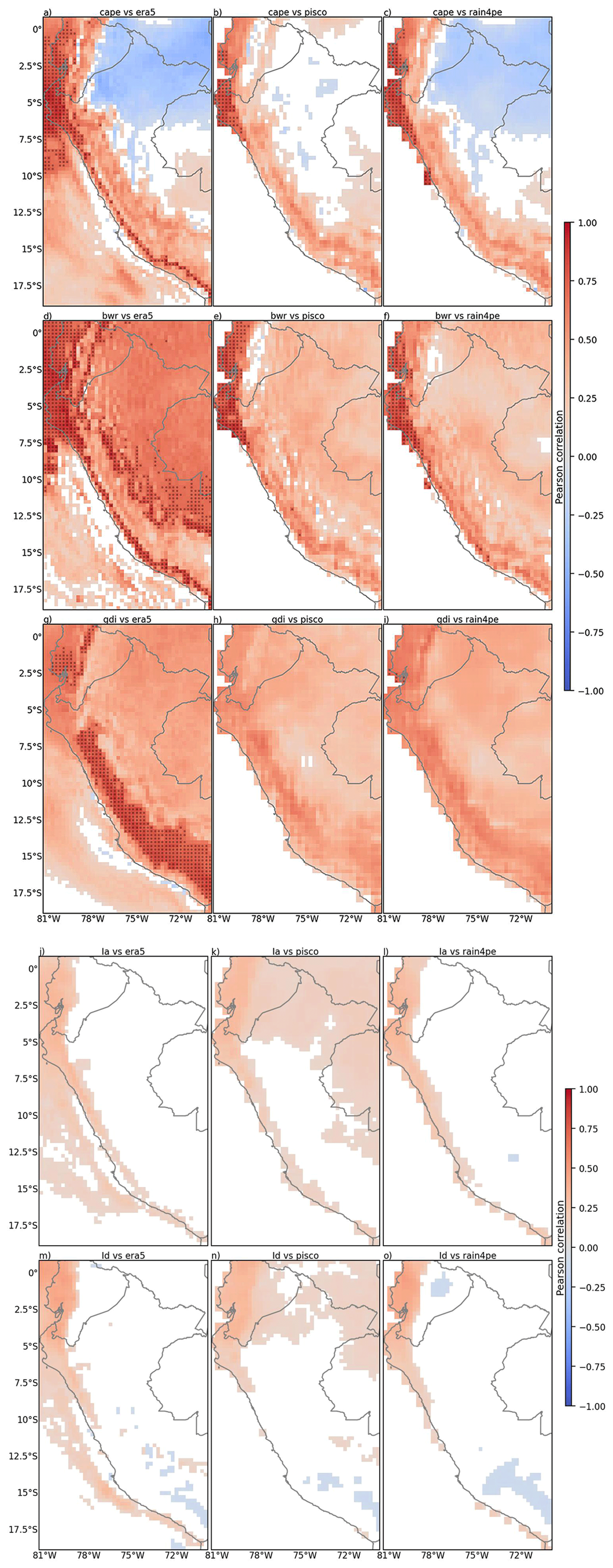
Figure 4 Pearson correlation (R) maps at the 95 % confidence level between monthly anomalies of convective indices (rows) and precipitation datasets (columns) for the 1981–2015 common period. The indices (rows) are (a–c) CAPE, (d–f) BWR, (g–i) GDI, (h–l) Ia, and (m–o) Id. The precipitation datasets (columns) are (a, d, g) ERA5, (b, e, h) PISCO, and (c, f, i) RAIN4PE. Shading is shown only for significant correlations (p-value <0.05). Red (blue) indicates positive (negative) R values. Gray points highlight strong correlations (R>0.7). Anomalies were calculated taking the 1981–2015 median as climatology.

Focusing on the critical coastal subdomain (Fig. 2b), the standardized scatterplots (Fig. 5) reveal that the BWR achieves the highest linear association and lowest dispersion among all evaluated indices. Unlike I_a and I_d, which show little relation to the intensity of anomalies, the BWR scales proportionally with precipitation magnitude. While the BWR calculation requires surface dew point temperature (T_d), which is tightly constrained by local oceanic boundary conditions (e.g., Niño 1+2 SST), the GDI fundamentally requires mid-tropospheric humidity (Gálvez and Davison, 2016). This distinction is critical because free-tropospheric moisture is highly sensitive to sub-grid convective parameterization schemes and remote advection, leading to substantial inter-model spread and systematic biases in climate models (John and Soden, 2007; Han et al., 2022). Unlike surface and boundary-layer variables, whose variance is physically anchored by local SSTs via the Clausius-Clapeyron relationship (John and Soden, 2007), mid-level humidity in climate models inherits significant uncertainty. Consequently, metrics dependent on free-tropospheric moisture could inherit more uncertainty for climate monitoring compared to surface-constrained proxies.

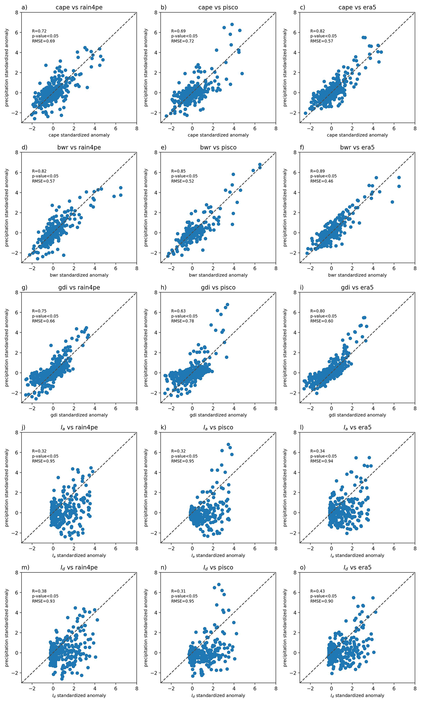
Figure 5 Scatterplots between convective indices and precipitation datasets over the NWSA adjacent to Niño 1+2. Scatterplots comparing monthly standardized anomalies of CAPE (a–c), BWR (d–f), GDI (g-i), (h–l) Ia, and (m–o) Id against standardized precipitation anomalies from ERA5 (left column), PISCO (middle column), and RAIN4PE (right column). All data are spatially averaged over the NWSA adjacent to Niño 1+2. The Pearson correlation coefficient (R) and the significance at the 95 % confidence level (p-value <0.05) are shown in each panel. The diagonal dashed line is the identity function.

The temporal evolution of the indices (Fig. 6) highlights specific strengths. The BWR outperformed other indices in capturing the magnitude of the extreme 1983 and 1998 El Niño events. For the 1998 event, the index aligned closely with precipitation observations, helping to resolve discrepancies between PISCO and RAIN4PE products. In the recent 2023 Coastal El Niño, all indices and ERA5 precipitation peaked in March–April; however, the PISCO product exhibited a sudden and physically unexplained decline in April. To validate the positive anomalies diagnosed by the BWR and ERA5 during this period, independent official climatological reports were consulted. Specifically, the National Meteorological and Hydrological Service of Peru (SENAMHI, 2023) and the Ministry of Agriculture and Livestock of Ecuador (MAG, 2023) documented significant positive rainfall anomalies along the northern Peruvian and southern Ecuadorian coasts during April 2023. Furthermore, during the 2024 dry event, PISCO showed a contradictory positive anomaly peak in April, whereas BWR, CAPE, and ERA5 precipitation consistently indicated negative anomalies according with observational monthly reports (SENAMHI, 2024; ERFEN, 2024). This independent observational consensus supports the physical consistency of the BWR, highlighting its value as a robust diagnostic tool.

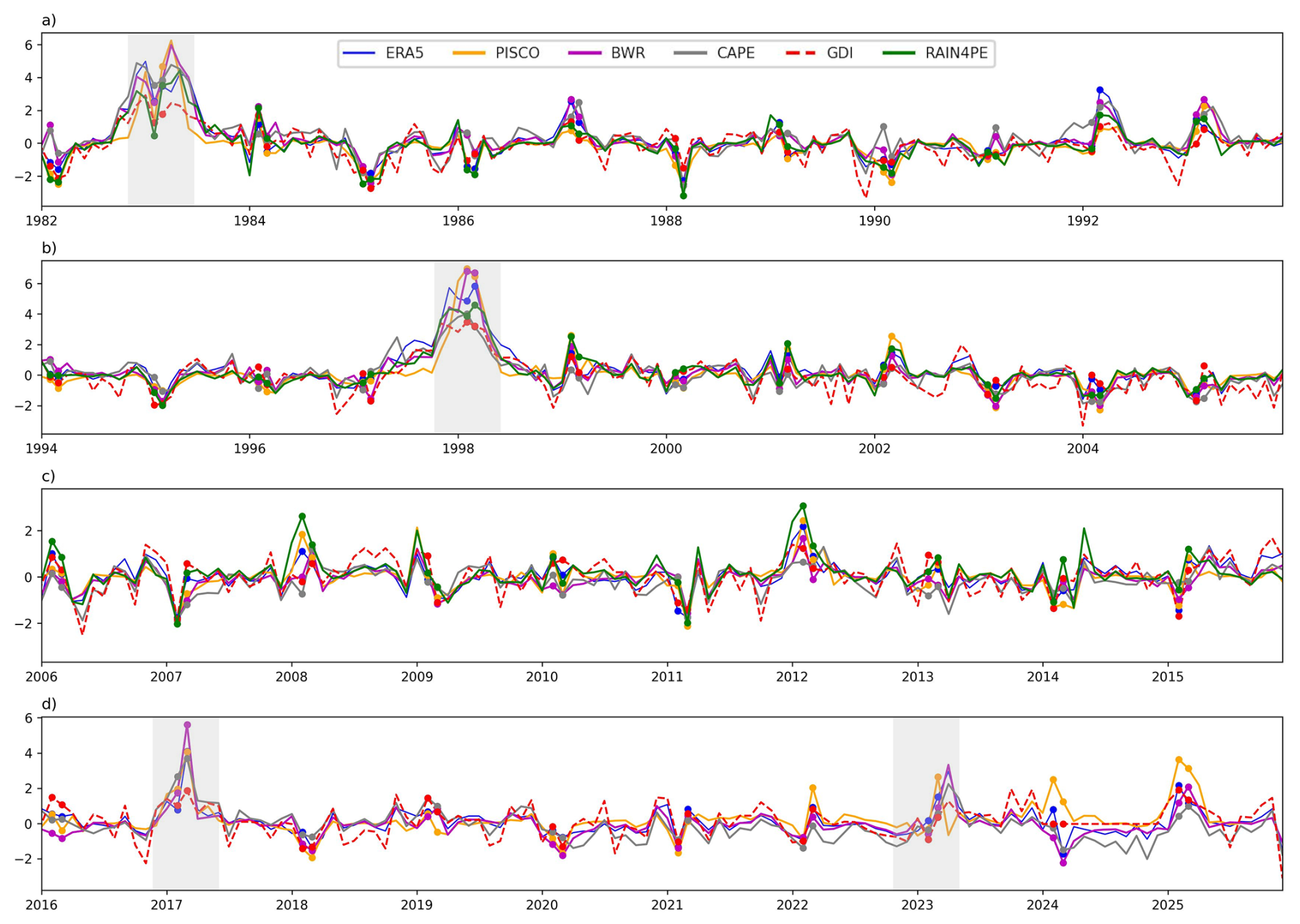
Figure 6 Time series of monthly standardized anomalies of convective indices, such as CAPE (gray), BWR (magenta), and GDI (dashed red), and standardized precipitation from ERA5 (blue), PISCO (orange), and RAIN4PE (green). All data are spatially averaged over the coastal subdomain (Fig. 2b) for the period 1981–2025. The RAIN4PE dataset is only available for 1981–2015. Anomalies were calculated taking the 1981–2015 median as climatology. Circle markers indicate February and March of every year. The vertical gray shadings show the four most extreme events: 1983, 1998, 2017 and 2023.

4.2 Causal discovery of precipitation in the NWSA

Figure 7a presents the reference causal network, constrained by the physical link assumptions described in Sect. 3.3.1. Although the causal directionality was a priori imposed to break the simultaneous circularity, the algorithm quantified the strength of these conditional dependencies. Such as, the SST over Niño 1+2 and the mesoscale vertical velocity (−ω₅₀₀) exert a strong control over atmospheric instability (ΔT_700−400) [MCI: 0.73] and precipitation [MCI: 0.61], respectively.

Building upon this reference, the second causal network (Fig. 7b) illustrates the system after the introduction of the BWR index. The resulting causal network confirms the preservation of the mesoscale thermodynamic and dynamic signals governing precipitation. Most importantly, the BWR index maintains a direct, robust causal link to precipitation [MCI: 0.60, with a confidence of 95.9 %] that exceeds the local evaporation signal [MCI: 0.25, with a confidence of 81.1 %]. This indicates that although local evaporation provides the necessary moisture for initial cloud formation, mid-level moisture advection plays a critical role in maintaining deep convection, and even helping to form the secondary band of the ITCZ (Aliaga-Nestares et al., 2023; Rivas Quispe et al., 2024), by mitigating the drying effect of environmental air entrainment and slowing down cloud evaporation (Sobel et al., 2001; Myoung and Nielsen-Gammon, 2010). Consequently, this validates the BWR formulation as a coherent physical integrator that couples the dominant dynamic with the thermodynamic, preserving the causal route to precipitation with significant strength [MCI: 0.60], even when the individual variables are algorithmically abstracted into the vertically integrated index (BWR).

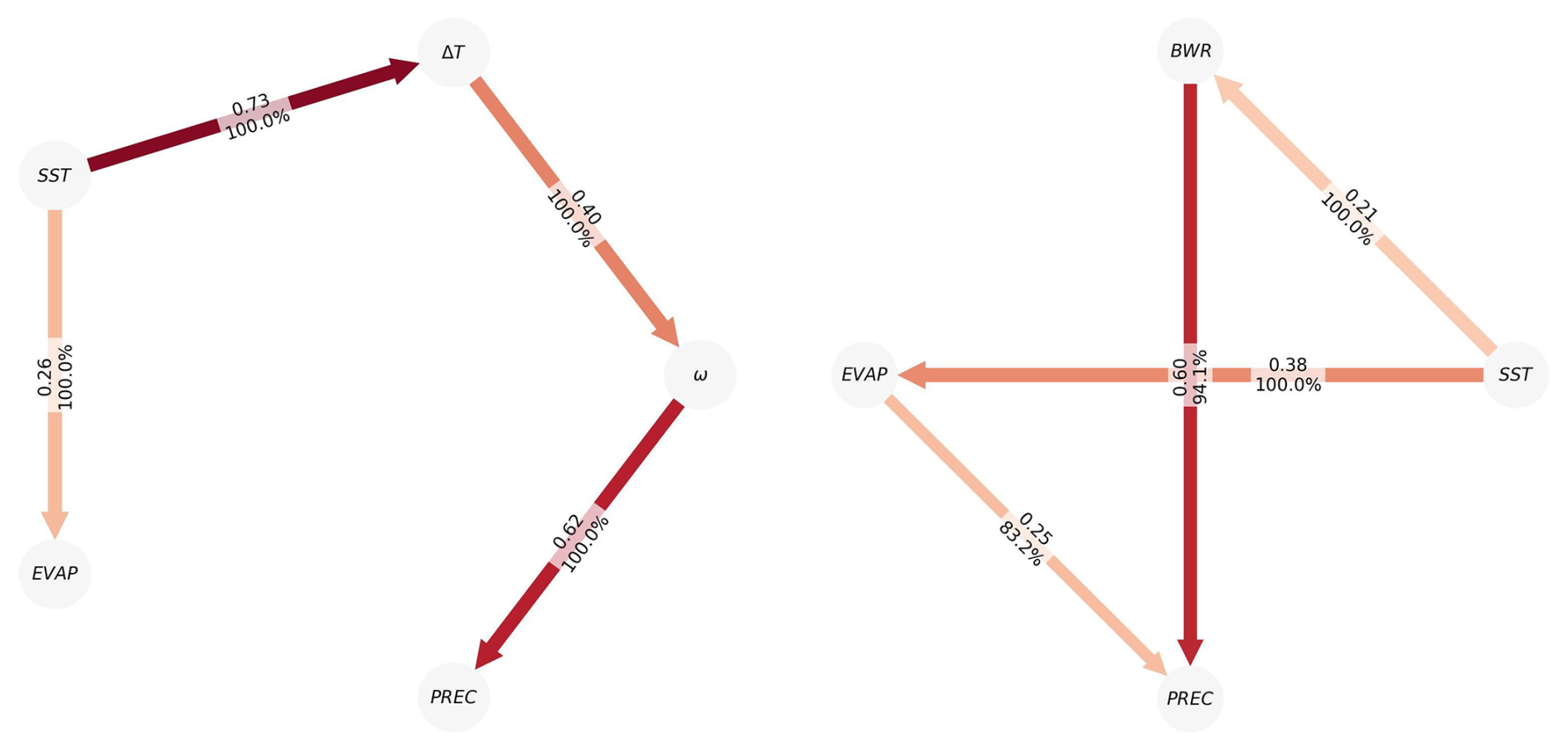
Figure 7 Causal networks without BWR (a) and with BWR (b). Red (blue) colors indicate direct (inverse) relationship. Darker (lighter) colors represent stronger (weaker) causal links. Arrows indicate the causal directions. Labels in middle of arrows indicate MCI (causal strength) values and their confidence of the 3000 bootstrap samples. All variables were averaged over the coastal subdomain (Fig. 2b), except precipitation, which was averaged only continentally, and SST, which was averaged over Niño 1+2 region. ω₅₀₀ and E values were inverted.

4.3 Physical mechanisms during extreme hydroclimatic anomalies

To characterize the atmospheric conditions associated with extreme hydroclimatic anomalies, March precipitation anomalies were analyzed over the coastal subdomain (Fig. 8). Based on the thresholds defined in Sect. 3.1, the rainiest (1983, 1993, 1998, 2002, 2017, 2022, 2023, and 2025) and driest (1982, 1985, 1988, 2003, 2011, and 2018) events were identified. As established in previous studies, these extreme precipitation responses are fundamentally governed by coastal El Niño and La Niña events, evidenced by SST anomalies in the Niño 1+2 region (Takahashi, 2004; Takahashi et al., 2018; Peng et al., 2024) (Fig. A2). Within this set, the 1998 and 2017 events are of particular interest as they encompass distinct oceanic dynamics driving similar precipitation extremes: while 1998 represents a canonical basin-wide extreme El Niño (Takahashi, 2004), 2017 manifested as a highly localized extreme coastal El Niño, characterized by intense warming strictly confined to the far-eastern Pacific despite weak La Niña conditions in the central basin (Takahashi et al., 2018; Peng et al., 2024). Additionally, the 2016 event was included as a contrasting case study because, despite prevailing strong global El Niño conditions, it lacked an extreme hydroclimatic response along the coast compared to the 1983 or 1998 events (Paek et al., 2017; Sanabria et al., 2019). This deviation underscores the notable influence that internal atmospheric variability can exert in altering regional teleconnections during distinct El Niño flavors (Huang et al., 2026).

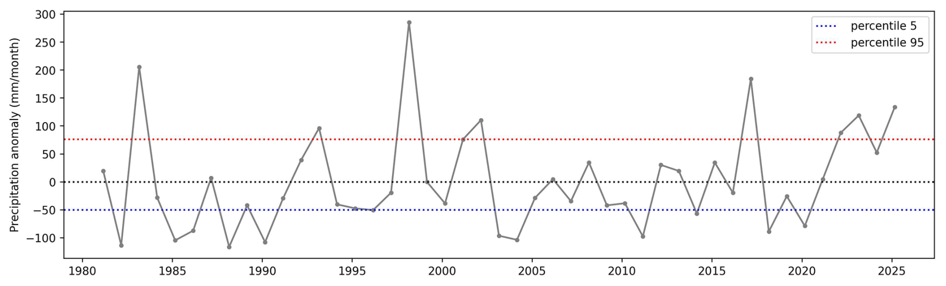
Figure 8 Monthly precipitation anomaly time series in March from PISCO, taking the 1981–2025 mean as climatology, averaged over the coastal subdomain. Precipitation above the 95th percentile and below the 5th percentile are considered as extreme hydroclimatic events.

4.3.1 Cross-section analysis in the coastal subdomain

During the 1998 and 2017 events, anomalous onshore westerly winds – driven by enhanced sea-breeze circulations – prevailed in the lower troposphere (Fig. 10f, k) (Takahashi, 2004; Rollenbeck et al., 2022). The collision of this flow against the western Andean slope near 80° W generated strong surface convergence. Consistent with the convergence feedback (Back and Bretherton, 2005), this near-surface forcing sustained a deep vertical ascent core extending from the surface up to 300 hPa. Finally, this convective column was ventilated in the upper troposphere (∼200 hPa) by easterly winds that induced strong divergence, completing the vertical circulation.

Concurrently with the onshore westerlies, the alongshore circulation exhibited a collapse of the climatological southerly winds (Takahashi, 2004). This relaxation permitted the intrusion of anomalous low-level northerly winds (Fig. 10f, k), consistent with the coastal dynamics described by Echevin et al. (2018) and Peng et al. (2019). Rather than a passive feature, these northerly flows acted as the primary driver for the coastal Bjerknes feedback (Peng et al., 2019) and the subsequent activation of the ITCZ southern branch (Takahashi and Martínez, 2017). Kinematically, this activation was captured as a robust convergence zone strictly confined between 6 and 3° S, which matches the established latitudinal limits of the active southern ITCZ band (Huaman and Takahashi, 2016). Finally, to balance this massive low-level mass convergence, the upper troposphere (200–100 hPa) responded with strong meridional divergence, effectively evacuating the ascending air northward and southward away from the convective core.

In contrast, the 2016 event showed a vertical descent core directly over the peak of the Andes (Fig. 9j). This subsidence was mechanically forced by upper-tropospheric convergence (∼300 hPa) induced by anomalous westerly winds – a teleconnection strictly consistent with the Central Pacific El Niño pattern identified by Sulca et al. (2017) – coupled with mid-level convergence (700–500 hPa) driven by easterly winds. This severe mid-level subsidence capped the atmospheric instability, keeping the region under stable, dry air as the descending branch of the Walker circulation failed to shift sufficiently eastward (Paek et al., 2017). As a consequence of this mid-level subsidence, the low-level convergence was neutralized, which can be identified as the absence of both northerly winds (Fig. 9j) and westerly sea-breeze (Fig. 10j), driving the severe moisture deficit and downward motion characteristic of this out-of-phase event (Sanabria et al., 2019).

To explicitly quantify how the dynamic constraints modulate the local thermodynamic potential, we examine the vertical profiles of ΔT, ω, and their product −ωΔT at the convective core boundary (79.75° W, 5° S; red star in Fig. 10f). Consistent with the deep convergence described previously, the extreme wet events of 1998 and 2017 exhibit a fully coupled atmospheric column. In these cases, atmospheric instability (ΔT) remains robust from 600 to 200 hPa and perfectly synchronizes with the maximum dynamic ascent (−ω), yielding peak −ωΔT values between 500 and 400 hPa (Fig. 11f, k). Conversely, the 2016 profile captures the exact top-down suppression identified in the cross-sections. Although substantial instability (ΔT) and localized ascent exist aloft (400–200 hPa), a severe layer of subsidence (ω>0) centered at 600 hPa physically severs the column, neutralizing the surface-to-upper-level connection and preventing deep convection (Fig. 11j). Furthermore, the driest events are systematically characterized by intense mid-level subsidence around 600 hPa. This persistent suppression is driven by the descending regional branch of the Walker Circulation (Sulca, 2021) and the stabilizing effect of negative SST anomalies (Fig. A2), which strengthen the coastal inversion (Rudloff et al., 2025). Ultimately, these vertical profiles confirm that while warm SSTs provide the necessary thermodynamic potential (Takahashi and Martínez, 2017), the convective outcome is strictly dictated by the mid-level dynamic response (Peng et al., 2019). Crucially, even without local oceanic cooling, teleconnected subsidence forced by Central Pacific warming can impose identical drying effects by capping the atmospheric column (Sulca et al., 2017; Paek et al., 2017).

As demonstrated by the contrasting outcomes of the 1998, 2017, and 2016 events, monitoring surface warming and low-level kinematics is insufficient to diagnose precipitation in dynamically limited regions like the NWSA. The mid-level dynamic environment (ω) ultimately dictates the convective response, either authorizing deep ascent or neutralizing the atmospheric column through subsidence. While this three-dimensional physical dependency is already recognized in the literature, routinely evaluating it requires complex, multi-level cross-sectional analysis. This highlights the practical need for a unified metric that explicitly couples the local thermodynamic potential with the mesoscale dynamic constraint. Consequently, the vertically integrated positive area of this product defines the BWR (Fig. 11), which acts as an explanatory proxy that could be useful for simplified monitoring and diagnosis, e.g. for using in a similar way as a stream-function (although not similar in its mathematical nature), condensing the complex 3D convective state into a rapidly interpretable 2D field.

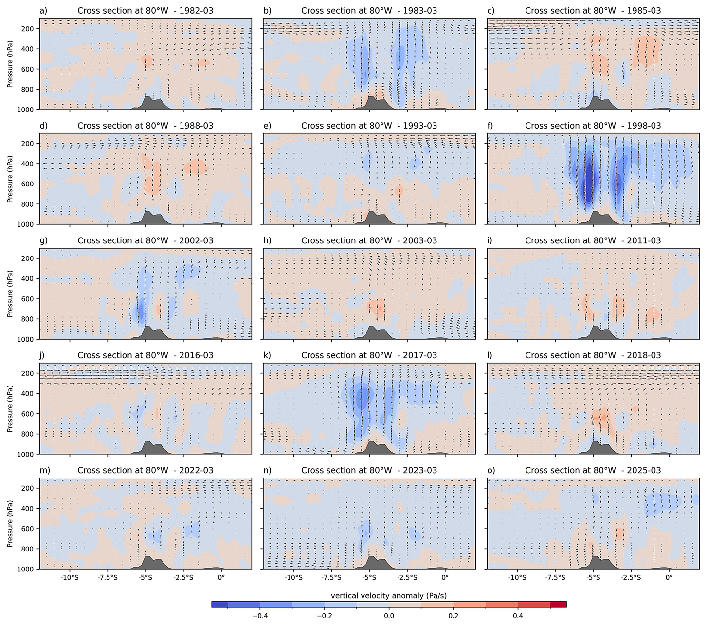
Figure 9 Latitudinal cross-section of the resultant vector between the anomalies of ω and meridional wind at 80° W, spanning from 12° S to 2° N, for the extreme hydroclimatic anomalies identified in Sect. 4. The blue (red) shaded colors indicate negative (positive) values of ω. The ω vector was multiplied by −20 to increase its scale and to get upward (downward) arrows with the air ascent (descent). Anomalies were calculated taking the 1981–2025 median as climatology.

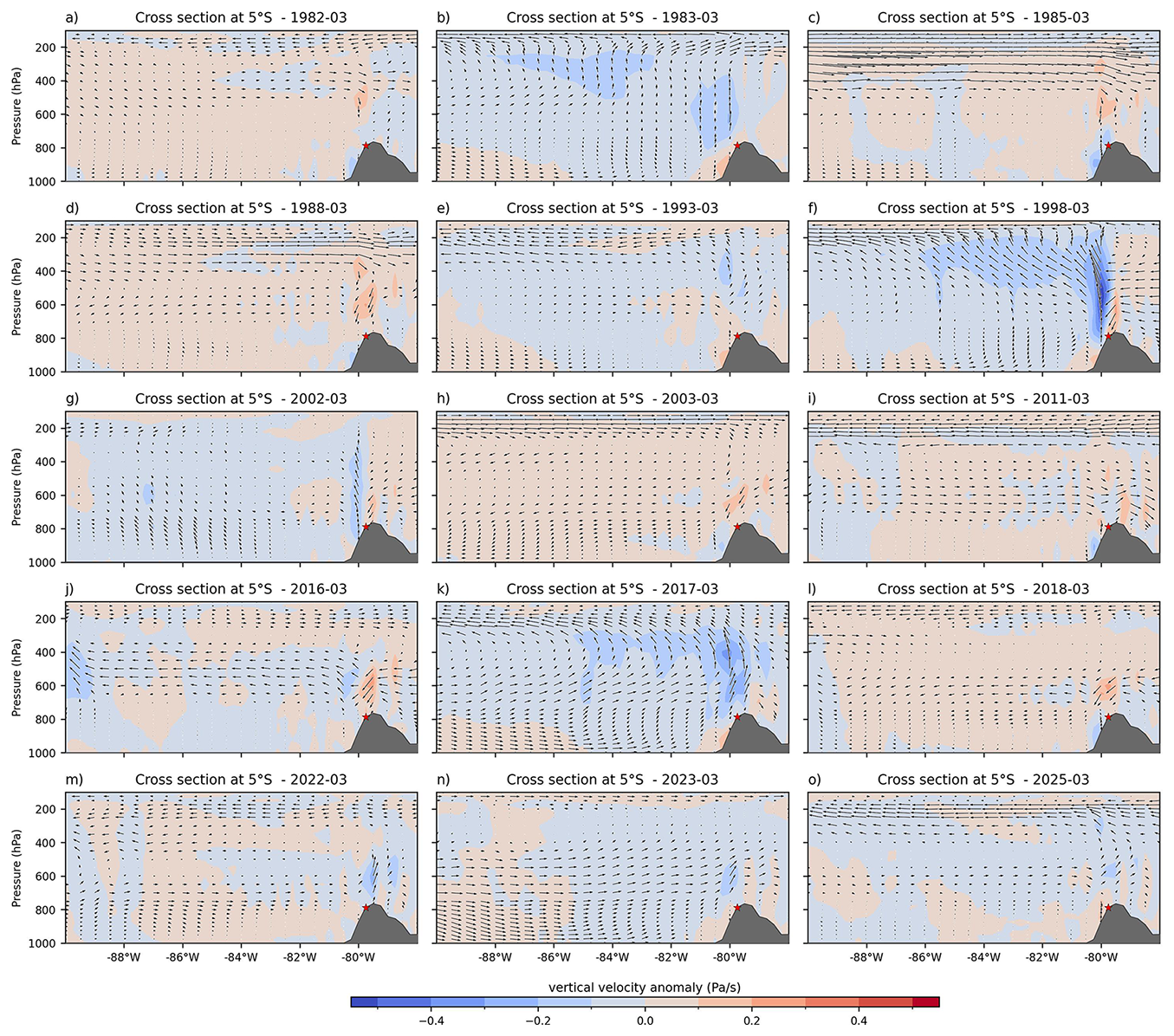
Figure 10 Longitudinal cross-section of the resultant vector between the anomalies of ω and zonal wind at 5° S, spanning from 90 to 78° W, for the extreme hydroclimatic anomalies identified in Sect. 4. The blue (red) shaded colors indicate negative (positive) values of ω. The ω vector was multiplied by −20 to increase its scale and to get upward (downward) arrows with the air ascent (descent). Anomalies were calculated taking the 1981–2025 median as climatology. Red star represents the longitude of the boundary between the ascent core and the descent core of the 1998 event.

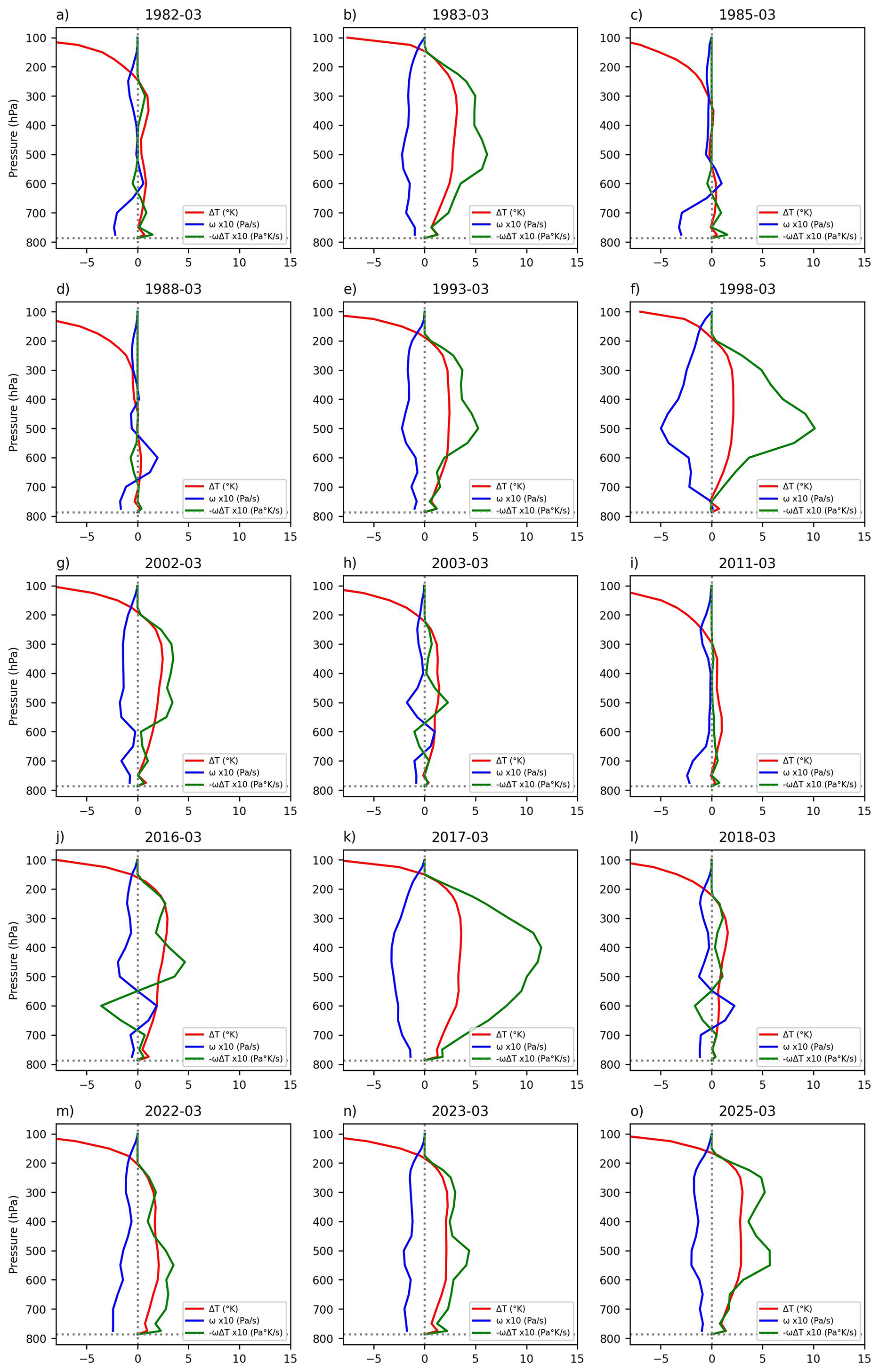
Figure 11 Profiles of ΔT (red), ω (blue) and −ωΔT (green) at (79.75° W, 5° S) for the extreme hydroclimatic anomalies identified in Sect. 4. The ω was multiplied by 10 to increase its scale. The horizontal dotted line shows the equivalent altitude of that point in pressure units. All variables share the same horizontal numerical axis.

4.3.2 BWR anomaly analysis

Building upon the vertical diagnoses from Sect. 4.3.1, the spatial distribution of the BWR anomalies (Fig. 12) maps the explicitly realized atmospheric response. As established in tropical dynamics (Cornejo-Garrido and Stone, 1977; Emanuel et al., 1994), large-scale vertical ascent (ω) and precipitation are inextricably coupled; diabatic heating from deep convection is fundamentally balanced by the adiabatic cooling induced by large-scale vertical motion. However, there is a critical physical distinction: while precipitation represents the localized thermodynamic output, ω represents the divergent circulation required to advectively export column-integrated moist static energy, dynamically maintaining the convective system (Neelin and Held, 1987). Consequently, by mathematically incorporating ω, the BWR is not a redundant empirical metric of precipitation, but an explicit physical quantification of the three-dimensional convective engine. In dynamically limited regions like the NWSA, where atmospheric instability (ΔT) is a necessary but insufficient condition for deep convection (Williams and Renno, 1993), this formulation is crucial. It physically discriminates actively coupled convective environments from those that are thermodynamically unstable but dynamically suppressed (Lau et al., 1997; Bony et al., 1997; DeMott and Randall, 2004). During the extreme wet events positive BWR anomalies dominated the coastal domain (Fig. 12b, e, f, g, k, m, n, o), being stronger in the 1998 and 2017 events, confirming the effective conversion of potential energy into kinetic energy. Conversely, the extreme dry events are characterized by widespread negative BWR anomalies (Fig. 12a, c, d, h, i, l).

The practical necessity of differentiating the localized thermodynamic output (precipitation) from the mesoscale mechanism of energy conversion (captured by the BWR) is empirically demonstrated by the 2016 event (Fig. 12j). During this strong Central Pacific El Niño, intense surface warming generated a high thermodynamic potential (ΔT>0), warning an extreme hydroclimatic event. However, the observed precipitation anomaly was near zero. While analyzing precipitation merely quantifies this lack of localized response (the effect), the BWR physically diagnoses the cause of the failure. Consistent with the vertical profiles from Sect. 4.3.1, the index yielded neutral to negative anomalies because it mathematically captured the structural decoupling of the atmospheric column: the atmospheric instability was neutralized by the mid-level subsidence (ω>0) imposed by the displaced Walker Circulation (Paek et al., 2017). Because atmospheric instability is a necessary but insufficient condition for deep convection (Williams and Renno, 1993), the BWR successfully filtered out this false positive. By explicitly diagnosing the dynamically suppressed environment, the BWR proves to be a more comprehensive diagnostic proxy for regional convection than isolated thermodynamic fields or precipitation outputs. Furthermore, for a more comprehensive diagnosis, it would be useful to overlay the divergent component of the wind or mid-level wind streamlines over the BWR anomaly maps, as this would explicitly visualize the 3D coupling between the vertical convective engine captured by the index and the mesoscale horizontal circulation.

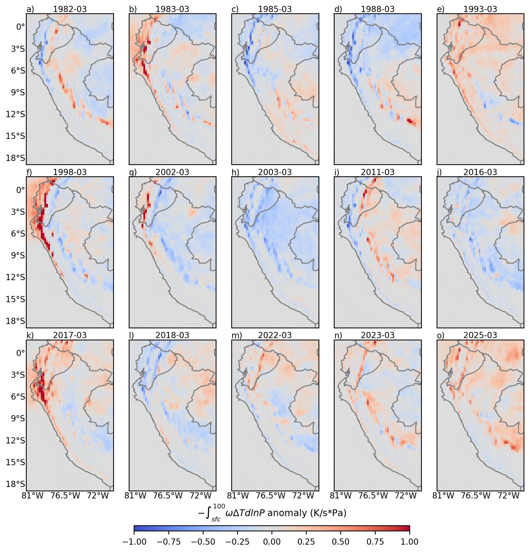
Figure 12 BWR anomaly, taking the 1981–2025 median as climatology, for the extreme hydroclimatic events identified in Sect. 4. The blue (red) shaded colors indicate negative (positive) anomalies of BWR.

4.4 Validation of extremes and signal persistence

To rigorously evaluate the robustness of the BWR during critical hydroclimatic phases, an Upper Tail Dependence (λ_U) analysis was conducted using empirical copulas. This approach quantifies the conditional probability that precipitation exceeds a high quantile given that the predictor index also exceeds the same quantile, providing a measure of asymptotic dependence essential for risk assessment. The copula space visualization (Fig. 13, left) exhibits a cross-like structure. While the main diagonal confirms the primary physical coupling, the anti-diagonal reveals regime mismatches in moderate conditions (e.g., false positives). However, the λ_U analysis (Fig. 13, right) demonstrates that this noise fades in the extremes. The λ_U coefficient increases for higher quantiles, peaking near 0.8 at the 97.5th percentile. This confirms strong asymptotic tail dependence: while the index may produce noise during moderate anomalies, it becomes a highly reliable diagnostic proxy specifically for the most extreme, potentially disastrous precipitation events.

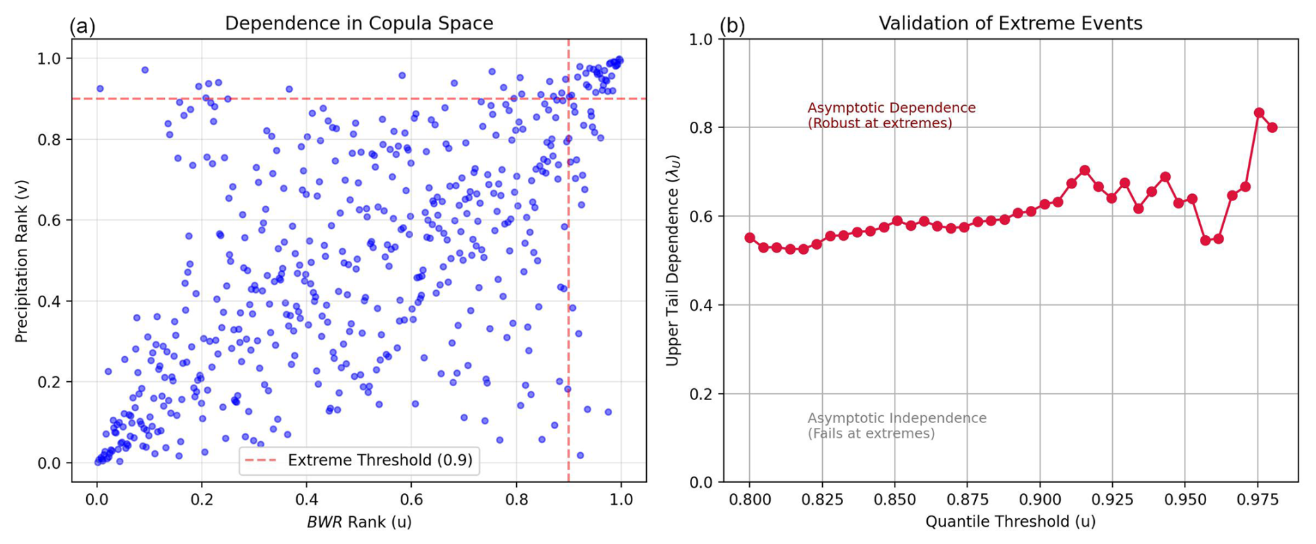
Figure 13 Analysis of the extreme dependence structure between BWR index and precipitation anomalies in the NWSA adjacent to Niño 1+2. (a) Scatterplot of pseudo-observations (uniform ranks) in the empirical copula space. The dashed red lines indicate the 0.90 quantile threshold; points in the upper-right quadrant represent concurrent extreme events. (b) The empirical Upper Tail Dependence Coefficient (λ_U) as a function of the quantile threshold (u).

While large-scale dynamic ascent (ω₅₀₀) alone might dictate instantaneous extremes, its utility for continuous monitoring is limited by its chaotic nature. This was assessed through a signal persistence analysis (Fig. 14). A rapid decorrelation was observed for ω₅₀₀ (blue line), which loses significant memory after short lags. In contrast, by integrating ΔT, the BWR (green line) mathematically inherits the thermal inertia of the oceanic boundary conditions. This integration effectively “anchors” the volatile dynamic signal to the slower-evolving thermodynamic state, yielding a predictability horizon significantly longer than that of pure ω₅₀₀. Thus, the BWR represents a physical trade-off: it sacrifices a marginal fraction of diagnostic precision at the extreme tail (compared to pure ω) to gain substantial signal stability and predictive capability, rendering it a highly practical tool for sub-seasonal to seasonal operative monitoring.

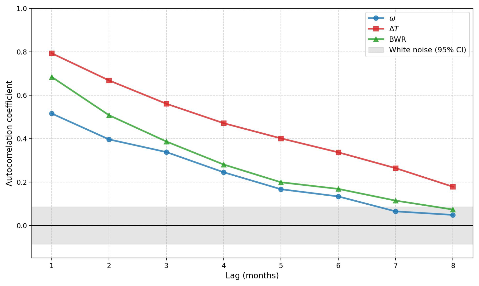
Figure 14 Analysis of signal persistence for the physical components of the BWR index. The plot displays the autocorrelation function (ACF) for vertical velocity (ω, blue), parcel buoyancy 400–700 hPa average (ΔT, red), and the BWR index (green) up to a lag of 8 months. The gray shaded area indicates the 95 % confidence interval for a white noise process ($\pm \mathrm{1.96}/\sqrt{N}$).

4.5 Predictive skill of the predicted BWR anomalies

During the peak of the rainy season (February–April), BWR anomaly predictions initialized in November and December exhibit a consistent improvement in predictive skill (ΔR≈0.1 to 0.2) compared with precipitation anomalies predicted by the ECMWF SEAS5 model (Fig. 15). Predicting precipitation anomalies in the NWSA during this critical hydroclimatic period is inherently complex due to the interaction between large-scale moisture convergence and the steep Andean topography (Garreaud, 2009; Trachte, 2018). Climate models often exhibit significant biases in these dynamically limited regimes because they rely on sub-grid convective parameterizations to generate local precipitation (Insel et al., 2009; Fernandez-Palomino et al., 2022). By substituting direct precipitation outputs with the BWR, the diagnosis circumvents these microphysical uncertainties. Instead, the BWR leverages the explicitly resolved large-scale vertical dynamics (ω) and thermodynamics (ΔT), which are governed by primitive equations and simulated with substantially greater fidelity by models (John and Soden, 2007; Emmenegger et al., 2024).

Furthermore, the BWR demonstrates a significant advantage for extended-lead predictions initialized in May, targeting the austral spring (October–November). At these 5- to 6-month lead times, the BWR anomalies yield marked correlation improvements (ΔR>0.3). This indicates that the BWR effectively retains predictive skill across the boreal spring predictability barrier. Because the BWR integrates the mesoscale atmospheric energetic conversion rather than relying on parameterized local rainfall, it provides a more robust and persistent proxy for the atmospheric state, confirming its operational utility for sub-seasonal to seasonal forecasting.

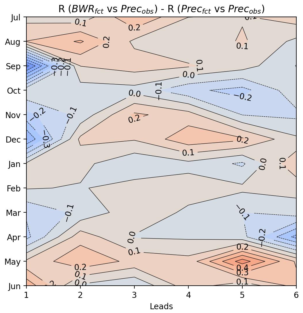
Figure 15 Predictive skill of BWR anomalies predicted up to a lead of 6 months. Shaded colors in red (blue) and contours with ΔR>0 (ΔR<0) represent better (worse) BWR predictive skill compared to the precipitation anomalies predicted by the SEAS5 model for the 2017–2025 operational period, using the PISCO dataset as the observational reference. The Y-axis represents the initial condition of the prediction.

5 Discussion

5.1 The Dynamic vs. Thermodynamic Control of Precipitation

The causal networks evaluated in Sect. 4.2 empirically support the physical hierarchy preserved by the BWR index, whose causal route to precipitation significantly dominates over other variables. This dominance is explained by the background dynamics of the region: although it is well established that local SST must exceed a specific threshold to trigger atmospheric instability (Woodman, 1999; Takahashi, 2004; Jauregui and Takahashi, 2018), in dynamically limited environments such as the coastal subdomain, this atmospheric instability (ΔT) is a necessary but insufficient condition for deep convection (Williams and Renno, 1993). Once the thermodynamic threshold is surpassed, control shifts predominantly to the mesoscale vertical velocity (ω) (Lau et al., 1997; Bony et al., 1997). Specifically, convection requires a mechanical trigger, such as the localized vertical ascent generated by the sea breeze colliding against the western Andean slope (Takahashi, 2004; Rollenbeck et al., 2022). This forced ascent lifts the air parcel to its Level of Free Convection (LFC), initiating latent heat release. Consequently, mid-level ω emerges to balance this diabatic heating through adiabatic cooling (Sobel et al., 2001), which, dictated by mass continuity, stimulates further low-level horizontal convergence, generating a circular causality known as convergence feedback (Back and Bretherton, 2005). By mathematically abstracting this dynamic mechanism, the BWR acts as a coherent physical integrator that successfully couples vertical velocity with atmospheric instability without losing the causal route to precipitation.

The BWR index mathematically abstracts this exact dynamic mechanism to operate in the dynamically limited environment of the coastal subdomain through the product of −ω and ΔT. This mathematical formulation acts as a physical constraint: the bidirectional feedback is only quantitatively realized when dynamic ascent ($-\mathit{\omega }>\mathrm{0}$) coincides with thermodynamic instability (ΔT>0). If the atmospheric column remains mechanically suppressed by the background subsidence (ω>0), the index zeroes out values, explicitly capturing the inability of local buoyancy to autonomously initiate the convective feedback loop.

The interaction between this thermodynamic potential and its dynamic realization fully explains the divergent regional responses observed during different El Niño flavors. While SST controls atmospheric instability, while SST gradients drive low-level horizontal convergence (Lindzen and Nigam, 1987; Lau et al., 1997; Bony et al., 1997). However, there are situations characterized by spatial and extensively homogeneous high SST values across the Pacific but with low SST gradients. This configuration translates into weak or null local convergence, as absolute high SSTs alone cannot force deep convection without the vertical ascent provided by spatial gradients (Lau et al., 1997; Sanabria et al., 2019) (e.g., the 2015–2016 El Niño). Conversely, asymmetric or high SSTs confined over smaller areas, such as the Niño 1+2 region (e.g., the 2017 and 2023 coastal El Niño events), generate strong SST gradients (Bony et al., 1997; Echevin et al., 2018; Aliaga-Nestares et al., 2023; Peng et al., 2024) that, initially, result in weak convergence, but when the convergence feedback is activated the convergence becomes stronger (Back and Bretherton, 2005), seamlessly converting thermodynamic potential into the extreme hydroclimatic anomalies physically diagnosed by the BWR.

5.2 Advantages of BWR as a physical diagnostic proxy

In dynamically limited environments like the NWSA coast, relying exclusively on thermodynamic indices yields high false-positive rates. As established by Williams and Renno (1993), thermodynamic instability (ΔT) is a necessary but insufficient condition for deep convection. When the regional Walker circulation imposes persistent subsidence, the atmospheric column remains mechanically suppressed despite intense surface warming. By mathematically coupling the thermodynamic potential with the vertical velocity (ω), the BWR acts as an explicit physical filter. It systematically zeroes out or yields negative values in thermodynamically unstable but dynamically suppressed environments, providing a selective diagnosis that purely thermodynamic predictors fail to capture (DeMott and Randall, 2004).

Furthermore, the BWR provides diagnostic capabilities that extend beyond observing precipitation anomalies. In atmospheric fluid dynamics, the conversion of available potential energy to kinetic energy requires the ascending of warm air and the descending of cold air. For the NWSA coast, this conversion mechanism has been specifically documented within the Lorenz energy cycle framework by Aliaga-Nestares et al. (2023). By computing the product of temperature anomalies (ΔT) and vertical ascent (−ω), the BWR functions as a direct two-dimensional proxy for this three-dimensional energy conversion. Therefore, the BWR explicitly quantifies the intensity of the convective forcing engine, whereas precipitation merely records the subordinated thermodynamic output.

Further, while the mid-level vertical velocity (ω) ultimately dictates the convective outcome, its high-frequency variability and rapid decorrelation limit its utility as an isolated monitoring index. The NWSA coastal climate is strongly constrained by the SST, which evolves slowly due to the ocean's large heat capacity and acts as a boundary condition for deep convection (Takahashi, 2004; Jauregui and Takahashi, 2018). By integrating ΔT, the BWR mathematically inherits this oceanic thermal inertia. The resulting hybrid index retains the rigorous dynamic constraint of ω required to prevent false positives, while acquiring the temporal stability of the oceanic forcing, making it an optimal proxy for sub-seasonal operative monitoring.

Finally, beyond its diagnostic utility, the operational advantage of the BWR becomes evident when applied to climate models for seasonal predictions. In topographically complex regions like the NWSA, climate models systematically exhibit biases because they rely on sub-grid convective parameterizations to estimate localized precipitation (Garreaud, 2009; Insel et al., 2009; Trachte, 2018; Fernandez-Palomino et al., 2022). By substituting native precipitation outputs with the BWR, the forecast circumvents these microphysical uncertainties. The index evaluates the large-scale vertical dynamics (ω) and thermodynamics (ΔT), which are governed by primitive equations and explicitly resolved with higher accuracy by the models (John and Soden, 2007; Emmenegger et al., 2024). Consequently, the BWR retains predictive skill at extended lead times and mitigates the forecast degradation caused by the boreal spring predictability barrier. By calculating the mesoscale atmospheric energy conversion rather than relying on parameterized rainfall, the BWR provides a physically robust proxy for operational predictions.

5.3 Physical limitations and interpretation of errors

It is acknowledged that the BWR, in its current formulation using vertical velocity (ω in Pa s⁻¹), does not possess strict units of power density (W m⁻²). However, its mathematical formulation (−ωΔT) is directly proportional to the generation term of Kinetic Energy (KE) from Available Potential Energy (APE) in the Lorenz energy cycle (Lorenz, 1955; Michaelides, 1987). By capturing the upward motion of warm air and the downward motion of cold air (Aliaga-Nestares et al., 2023), the index functions as a kinematic quantification of the energy conversion rate within the atmospheric column.

Despite the robust performance of the BWR during extreme events, significant limitations exist in moderate convective regimes, as evidenced by the dispersion observed in the copula space (Sect. 4.4). These limitations stem directly from the index's simplified formulation. First, the BWR lacks an explicit humidity term. The index assumes that the product −ωΔT leads to latent heat release (Q), consistent with the tropical energy balance where Q is primarily balanced by adiabatic cooling (Cornejo-Garrido and Stone, 1977). However, in cases of “dry ascent”, where strong dynamic lifting occurs in a moisture-starved environment, Q is limited by moisture availability rather than vertical motion. Consequently, the BWR yields false positives, measuring the intensity of the circulation's “engine” but not the efficiency of its output. Second, because the BWR is integrated from the surface to 100 hPa to strictly isolate deep convection, it systematically generates false negatives for precipitation driven by shallow convection or warm rain processes, which do not involve deep tropospheric ascent. Third, the current formulation lacks a high-frequency spatial filter. At native grid resolutions, the ω field inherently convolves the large-scale background dynamics with localized kinematic responses. While filtering the smaller horizontal scales in ω would isolate the large-scale environment to formulate a more transparent metric of precursor conditions leading eventually to precipitation anomalies, the current unfiltered index operates fundamentally as a diagnostic proxy of the realized convective state. Future efforts to further optimize the BWR will explore the application of spatial filters to the ω field.

Consequently, the translation of the BWR to other tropical latitudes imposes strict physical boundaries. Over continental regimes like the Amazon basin (Fig. ), deep convection is primarily constrained by convective inhibition (CIN) (Fu et al., 1999). Because the BWR evaluates dynamic forcing and positive buoyancy without accounting for the energy required to overcome CIN, its diagnostic correlation decreases significantly in these environments. Furthermore, over the eastern slopes of the Andes, precipitation is frequently driven by localized mechanical orographic lifting under conditions of weak large-scale ω (Trachte, 2018). These highly localized mechanical processes are unresolved at the spatial resolution of current global reanalysis data (Insel et al., 2009; Fernandez-Palomino et al., 2022), which physically exacerbates the generation of false negatives.

Beyond the tropics, the application of the BWR becomes physically inconsistent. In the midlatitudes and subtropics, atmospheric dynamics are predominantly governed by baroclinic instability, frontal lifting, and strong Coriolis forcing (Sobel et al., 2001). Applying the BWR directly to extratropical regimes misrepresents the fundamental energy conversion processes driving precipitation in those latitudes. Finally, it must be reiterated that the BWR is fundamentally a diagnostic proxy of the macro-scale convective environment, not a direct measure of precipitation physics. The Tail Dependence analysis confirms that while the index's simplified formulation introduces noise during moderate conditions, these limitations become secondary during extreme events, where intense dynamic forcing and boundary-layer instability strictly dominate the atmospheric response.

6 Conclusions

In dynamically limited environments such as the coastal NWSA, thermodynamic instability (ΔT) alone is insufficient to autonomously trigger deep convection due to persistent background subsidence. The BWR addresses this boundary constraint by vertically coupling ΔT and vertical velocity (ω). The causal discovery analysis (PCMCI+) empirically verified this formulation, demonstrating that the BWR preserves the dominant causal route to precipitation over other individual thermodynamic or dynamic variables, capturing the dynamic trigger required to realize convection. Furthermore, the upper tail dependence analysis based on empirical copulas confirmed the index's robustness during climate extremes. While isolated thermodynamic variables exhibit asymptotic independence, the BWR demonstrates strong asymptotic tail dependence, proving to be a highly reliable diagnostic specifically for the most extreme hydroclimatic events.

As a diagnostic proxy, the BWR systematically outperforms established thermodynamic indices because it explicitly quantifies the realized mesoscale atmospheric response rather than just the precursor potential. Furthermore, while isolated mid-level vertical velocity dictates instantaneous convection, its high-frequency volatility limits its utility for monitoring. By integrating ΔT, the BWR mathematically inherits the thermal inertia of the oceanic boundary conditions. This integration imparts greater signal persistence to the index, making it a slightly more stable proxy for sub-seasonal operative monitoring.

Ultimately, the operational value of the BWR emerges in its prognostic application. By substituting predicted precipitation anomalies from SEAS5 with the predicted BWR anomalies, the predictions slightly overcome the limitations of the sub-grid parameterization inherent in the model. Relying instead on explicitly resolved mesoscale variables governed by primitive equations, the BWR systematically improves seasonal predictive skill during the peak of the austral summer and mitigates the forecast degradation caused by the boreal spring predictability barrier.

Appendix A

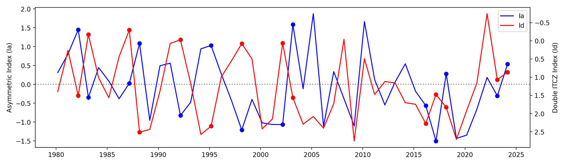
Figure A1 Time series of the March Ia and Id indices for the period 1981–2025 taking the same areas proposed by Aliaga-Nestares et al. (2023).

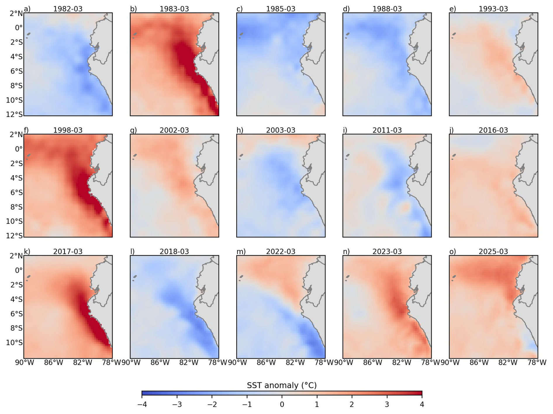
Figure A2 SST anomaly over the Niño 1+2 region from ERA5 for the extreme hydroclimatic events identified in Sect. 4. The blue (red) shaded colors indicate negative (positive) anomalies of SST. Taking the 1981–2025 median as climatology.