The impact of stochastic sea ice perturbations on seasonal forecasts

Sea ice ensemble forecasts can be highly underdispersive, meaning that the ensemble spread is notably lower than the average forecast error. One common strategy to address underdispersion is to add stochastic perturbations to the forecasts. We detail the implementation of a stochastically perturbed parameterisation (SPP) scheme for SI³, the sea ice component used by the Integrated Forecast System (IFS), the forecast model used and developed by the European Centre for Medium-Range Weather Forecasts (ECMWF). We then evaluate its impact on seasonal forecasts of Northern Hemisphere summer and winter. The inclusion of SPP is found to enhance ensemble spread for sea ice concentration (SIC) and sea ice thickness (SIT) forecasts by around 10 % relative to a forecast with no SPP, which results in a better calibrated probabilistic forecast. Some small but robust changes to the mean state are also found, including a general decrease in the mean SIC and a redistribution of the winter ice from the central Arctic to the ice edge. These changes reduce or increase the mean bias depending on the region. Changes to the mean and spread of the sea ice result in changes to the mean and spread of air temperature up to at least 850 hPa, altering the mean air temperature biases of the model. An apparent consequence of this is a significant increase in the anomaly correlation coefficients of 500 hPa geopotential height (Z500) over the Euro-Atlantic domain in winter, which partially projects onto the North Atlantic Oscillation. We conclude that sea ice stochastic perturbations can be a valuable contribution to increased reliability of seasonal forecasts of the sea ice itself and can impact seasonal forecasts of the atmosphere at high and mid latitudes.

1 Introduction

In the context of numerical weather prediction (NWP) and climate modeling, a stochastic parameterisation scheme is a way to insert random perturbations into the model in a controlled way. Such perturbations are appealing for two reasons. Firstly, no matter the model resolution, there will always be fluctuations in the system arising from unresolved sub-gridscale processes, and due to the non-linear nature of the governing equations they can still exert a non-zero net effect on the large-scale flow (Palmer, 2012). Even in cases where the physical parameterisation included to represent such processes is considered reasonable, there are inevitably free parameters in such parameterisations that cannot be tightly constrained from data, and the associated uncertainty can again ripple out to the large-scale. Unresolved sub-gridscale processes are therefore a potential source of model biases. Secondly, NWP models often produce ensemble forecasts that are underdispersive (i.e., the ensemble distributions do not have enough spread relative to typical forecast errors). Stochastic parameterisation schemes, or just stochastic schemes for short, address both of these concerns. The injected noise aims to represent the unresolved processes, with a practical effect being an often substantial increase in ensemble spread. The potential for such schemes to thereby improve probabilistic weather forecasts is well known (Palmer et al., 2009; Sanchez et al., 2015; Berner et al., 2017; Lang et al., 2021; Xu et al., 2022). ECMWF has been using stochastic schemes for the atmosphere in operational ensemble forecasts since 1998 (Buizza et al., 1999). The original stochastically perturbed parameterisation tendency (SPPT) scheme has recently been replaced by one based on stochastically perturbed parametrisations (Leutbecher et al., 2024).

While most applications have focused on perturbing the atmospheric component of the model, stochastic schemes have also been implemented in the land (MacLeod et al., 2016), ocean (Brankart et al., 2015; Juricke et al., 2017; Storto and Andriopoulos, 2021), sea ice (Juricke et al., 2013; Juricke and Jung, 2014) and dynamical core (Subramanian et al., 2019) components of NWP and climate models. The effect of combining multiple such schemes was documented in Strommen et al. (2019). Here, we will focus on stochastically perturbed sea ice.

The idea of adding stochastic perturbations to the sea ice is particularly attractive, as sea ice forecasts are often systematically underdispersive, even (in fact, especially) at the time of initialization (Dirkson et al., 2019, 2022; Peterson et al., 2022). This is likely related to the typically large biases models exhibit in sea ice (Notz and SIMIP Community, 2020) and the importance of unresolved or poorly modelled sea ice and boundary layer processes. Juricke et al. (2014) found that ensemble spread on the sub-seasonal timescale can indeed be enhanced by including stochastic perturbations to the ice strength parameter P^*, and to a lesser extent on seasonal timescales. Juricke and Jung (2014) showed that such perturbations can also change the mean state in the polar regions, despite being mean-zero, which they ascribed to asymmetries in the response of sea ice to P^* perturbations. Their analysis generally highlighted some of the complex phenomena arising when adding sea-ice perturbations to a model, including potential differences in coupled vs. uncoupled simulations (owing to the important effects of ice-ocean-atmosphere coupling) and the different timescales of the response (with a potentially multidecadal transient adjustment of the ice). Strommen et al. (2022) corroborated such changes to the mean and variability of sea ice, while also highlighting the prospect for stochastic perturbations to improve ice-ocean-atmosphere coupling and, as a result, seasonal timescale teleconnections from the Arctic to the mid-latitudes. As a result, it is possible that stochastic sea-ice perturbations could affect forecast skill, not just for sea-ice forecasts but also atmospheric forecasts. The potential importance of sea ice at driving midlatitude atmospheric variability has been highlighted in several past papers (Kretschmer et al., 2016; Wang et al., 2017).

The goal of this paper is to evaluate the implementation of a stochastic parameterisation scheme to SI³, the sea ice component used by the Integrated Forecasting System (IFS), the forecast model used and developed by the European Centre for Medium-Range Weather Forecasts (ECMWF). The scheme used is a modified version of the one described in Storto and Andriopoulos (2021), which is based on parameter perturbations, following the ideas of Juricke et al. (2013). This approach ensures consistency with the approach taken to stochastic perturbations in the atmospheric component of the IFS, which has the advantage of being conservative of tracers, momentum, and sea ice volume, unlike alternative perturbation schemes based on tendency or energy perturbations (Lang et al., 2021; Leutbecher et al., 2024).

We will first of all detail the scheme used and report on experience gained from various sensitivity tests, which informed the choice of a default configuration. Then we will examine the impact of this default configuration on ensemble forecasts in the IFS, including the basic impact on the mean state and ensemble spread of sea ice concentration (SIC), sea ice thickness (SIT), and air temperature, as well as how forecast skill is affected in both the ice and atmosphere. We also include analysis concerning to what extent changes to the mean and spread of sea ice are related, which is relevant for applications where it is desirable to minimise mean state changes without compromising enhanced spread. Finally, we provide a discussion on what next steps are suggested by our results.

The focus of the analysis will be on the Arctic and northern midlatitude summer and winter. Impacts on Antarctica are included at the end of the Supplement. We will almost exclusively present results for seasonally averaged fields, thereby omitting analysis focused on the temporal evolution of SPP-induced changes. Such analysis will instead be included in a follow-up study assessing the impact of SPP in sub-seasonal forecasts.

2 Data and Methods

2.1 Model simulations and observational data

We examine the impact of stochastic sea ice perturbations using a prototype version of cycle 49R2 of the IFS. Cycle 49R2 is internal and under development at the time of writing. It forms the basis for the next generation of ECMWF reanalysis, ERA6, as well as the new seasonal forecast system, SEAS6, replacing the former SEAS5 system (Johnson et al., 2019). The exact configuration we used is close to the final version of SEAS6. Documentation for cycle 49R1 can be found here: https://www.ecmwf.int/en/publications/ifs-documentation (last access: 24 August 2026). Cycle 49R2 differs from 49R1 primarily by coupling to version 4 of NEMO and the new SI³ sea ice model (Gurvan et al., 2019; Vancoppenolle et al., 2023). SI³ is a state-of-the-art sea ice modelling system including a subgrid-scale ice thickness distribution with five ice thickness categories, each with four thermodynamic layers and a single snow layer on top. There is also prognostic sea ice salinity, simulation of melt ponds, and better representation of snow on sea ice. An informal discussion of the use of NEMO-SI³ with the IFS, and improvements relative to the previous system using NEMO3.4-LIM2, can be found in Keeley et al. (2024). The IFS is run using the Tco199 cubic octahedral grid, corresponding to a grid spacing of around 50 km at the equator, with 137 levels in the vertical. NEMO-SI³ is run with a horizontal resolution of 0.25° using the eORCA025 tripolar grid. The size of the grid boxes in the polar regions is around 15 km on average with some cells as small as 3km. There are 75 levels in the vertical. Both the IFS and NEMO-SI³ are run using single-precision arithmetic, and the IFS has atmospheric stochastic perturbations active (Lang et al., 2021; Leutbecher et al., 2024).

We then generate 50-member ensemble forecasts using this model configuration. The ensembles are initialised on 1 November and 1 May for every year between 1993 and 2023 inclusive, and run for 6 months, thereby covering the full winter and summer seasons. The ensemble of 50 atmospheric initial conditions is based on ERA5 (Hersbach et al., 2020) using ensemble data assimilation (Buizza et al., 2008) and singular vector perturbations (Leutbecher and Palmer, 2008). For the ocean and sea ice, an ensemble of 11 initial conditions is used based on the new Ocean Reanalysis System 6 (ORAS6) developed at ECMWF (Zuo et al., 2025; Browne et al., 2026). A paper describing ORAS6 in detail is still in preparation: see Zuo et al. (2017) and Zuo et al. (2019) for documentation on the older ORAS5 system. The 11 ocean initial conditions are then repeated sequentially to a total of 50. Two sets of such ensembles are generated. The first is our “control” run (referred to as CTRL), and the second differs from this control only in its inclusion of stochastic sea ice perturbations (referred to as SPP). These perturbations are described in Sect. 3. We emphasise that the generation of the ocean and sea ice initial conditions does not make use of the sea ice SPP scheme. SPP is therefore only affecting the forecast itself. The possibility of applying SPP to boost initial condition spread will be discussed later.

In our analysis we will primarily be comparing the CTRL and SPP forecasts for the northern hemisphere winter (December–January–February, DJF) and summer (June–July–August, JJA) seasons. For observations, there can be substantial uncertainty in the production of sea ice concentration analysis obtained from remotely sensed proxies (e.g., satellite radiances), and different products may therefore have non-trivial differences. Here we use the Global Sea Ice Concentration climate data record (SMMR/SSMI/SSMIS) from EUMETSAT OSI-SAF (https://doi.org/10.15770/EUM_SAF_OSI_0013, EUMETSAT OSI SAF, 2022a) until 2020 and its extension OSI-430-a (https://doi.org/10.15770/EUM_SAF_OSI_0014, EUMETSAT OSI SAF, 2022b) from 2021 onwards. For verification of atmospheric variables, we use ERA5 reanalysis.

2.2 Metrics and statistical methods

Let x_t,k denote an ensemble forecast at lead-time t with k = $\mathrm{1},\mathrm{\dots },K$ ensemble members, and let y_t denote the verifying observations. Let $\stackrel{\mathrm{‾}}{x_t}$ denote the ensemble mean forecast. Given N such distinct forecast, we evaluate the forecast skill using several metrics. The ensemble spread is the standard deviation ${\mathit{\sigma }}_{x_k}$ computed over all members. The root-mean-square-error (RMSE) is

$$\begin{array}{}\text{(1)}& \text{RMSE}=\sqrt{{\displaystyle \frac{\mathrm{1}}{N}}\sum _t{\left(\stackrel{\mathrm{‾}}{x_t}-y_t\right)}^{\mathrm{2}}}.\end{array}$$

The spread-error ratio is the square root of the average ensemble variance (computed using the sample variance formulation with 1 degree of freedom) divided by the RMSE, with an additional correction factor to address the finite ensemble size (Roberts and Leutbecher, 2025):

$$\begin{array}{}\text{(2)}& \text{Spread/Error}=\sqrt{{\displaystyle \frac{K+\mathrm{1}}{K-\mathrm{1}}}}{\displaystyle \frac{\sqrt{\frac{\mathrm{1}}{N}\sum _t{\mathit{\sigma }}_{x_k,t}^{\mathrm{2}}}}{\text{RMSE}}}.\end{array}$$

If the forecast is reliable in a probabilistic sense, i.e., if ensemble members and verification are exchangeable, then the expected value of this ratio is 1 (Fortin et al., 2014). Values close to 1 therefore indicate high reliability and values close to 0 indicate low reliability. For an additional measure of probabilistic forecast skill, we use the continuous ranked probability score (CRPS); see, e.g., Hersbach (2000). The CRPS for a single forecast at time t is

$$\begin{array}{}\text{(3)}& {\text{CRPS}}_t={\displaystyle \frac{\mathrm{1}}{K}}\sum _k\left|x_{t,k}-y_t\right|-{\displaystyle \frac{\mathrm{1}}{\mathrm{2}{K}^{\mathrm{2}}}}\sum _i\sum _j\left|x_{t,i}-x_{t,j}\right|,\end{array}$$

and the overall CRPS is CRPS_t averaged over all cases t. Informally, the CRPS is a generalisation of the mean-squared error which assesses the performance of the ensemble as a whole, as opposed to just of the ensemble mean. It is positive definite, and lower values indicate better performance.

In this paper a primary focus is on assessing improvements to forecast skill, especially probabilistic skill, when including SPP. However, mean model biases can often dominate skill metrics, especially for sea ice. The above skill metrics are therefore computed using the bias-corrected fields. This is done by first computing the season-dependent mean bias over all times t, $\frac{\mathrm{1}}{N}{\sum }_t\left(\stackrel{\mathrm{‾}}{x_t}-y_t\right)$, and then subtracting this from every ensemble member before computing the RMSE and CRPS. Finally, in the case of Z500 we will also measure forecast skill using the Pearson correlation between $\stackrel{\mathrm{‾}}{x_t}$ and y_t, typically referred to as the anomaly correlation coefficient (ACC).

To test statistical significance of changes between two forecasts, we use a two-tailed t test when testing changes to the ensemble mean, and a Bartlett test to test changes to the ensemble spread. We use a two-tailed t test to estimate significance for a single correlation being non-zero. To assess significance of changes to the ACC between CTRL and SPP, we use the “three-way-correlation test” from Siegert et al. (2017), which accounts for the presence of covariance between two different forecasts of the same event. We will be testing for such differences at multiple gridpoints at once, which introduces the risk of a multiple testing fallacy. We account for this in two ways. Firstly, we apply a false discovery rate correction due to Benjamini and Hochberg (1995), which applies a blanket correction to the spatial field of p values. Secondly, we use Monte Carlo resampling to construct a null distribution, representing the null hypothesis that there is no real difference in correlations between the control and the SPP experiment: the time order of the verifying observations is randomly shuffled, and the p values for the change in correlations are recomputed. This breaks the physical forecast-observation relationship while preserving the spatial structure of the observations and the shared structure between CTRL and SPP. Repeating the procedure many times allows estimating how often apparently significant differences would occur by chance, while accounting for spatial correlation. All these tests were primarily implemented using the python package scipy (Virtanen et al., 2020).

All data used has been regridded to the same regular 1° grid prior to analysis being carried out.

3 The stochastic perturbation scheme

The scheme used is the stochastically perturbed parameterisation (SPP) scheme implemented in the STOPACK package described in Storto and Andriopoulos (2021), extended to allow more sea ice parameters to be perturbed. A similar SPP scheme is already used in the atmospheric component of the IFS (Ollinaho et al., 2017; Lang et al., 2021). While STOPACK allows for several different types of parameter perturbation, the default one used here is based on log-normal perturbations obtained by drawing numbers from a random field evolving in space and time. This is similar to the scheme originally developed by Stephan Juricke and others (Juricke et al., 2013).

Concretely, a random noise field covering all gridpoints is first generated by repeatedly applying a Shapiro filter (Shapiro, 1970) to an initial random white noise field 𝒲. The filter introduces lengthscales (i.e., correlations in space), the size of which is a function of the number of iterations: Fig. S1 in the Supplement shows this function. Call the resulting noise field 𝒫. Then 𝒫 evolves in time according to an autoregressive process with a lag of 1 day. At every time step, given a parameter p, a perturbed parameter $\widehat{p}$ is then generated at each grid-point according to the formula

$$\begin{array}{}\text{(4)}& \widehat{p}=p\cdot \exp \left({\mathit{\xi }}_t\right),\end{array}$$

where ξ_t is value of the random field 𝒫 at that grid-point at that point in time. The initial white noise field 𝒲 used to generate the random field is chosen to be $\mathcal{N}\left(-\frac{\mathrm{1}}{\mathrm{2}}{\mathit{\sigma }}^{\mathrm{2}},{\mathit{\sigma }}^{\mathrm{2}}\right)$. The choice of the mean here ensures that the mean value of $\widehat{p}$ is p. The value of σ, the standard deviation, is a free parameter determining the magnitude of perturbations. The current implementation of SPP uses 250 iterations of the Shapiro filter to generate the random field, corresponding to a lengthscale of around 750 km. The decorrelation timescale of the field is set to 10 d.

Importantly, in the current implementation of SPP, all perturbed parameters share the same random field. In future iterations of the scheme we intend to shift towards independent random fields for each parameter, for more consistency with the approach taken in the atmospheric SPP. In the present work we use such independent fields in precisely one isolated case (see Sect. 4.3). Producing multiple such random fields in a computationally efficient way necessitated the use of a more efficient algorithm than iterated Shapiro filters, and therefore we use the Perlin Noise algorithm for this (Perlin, 2002). The Perlin noise algorithm produces spatially correlated random fields through gradient interpolation on a regular lattice. We used a lattice comprising 15 and 12 cells in the latitude and longitude directions, respectively. Length scales are introduced using two octaves of noise, with a lacunarity of 2 governing the frequency increase between octaves and a persistence value of 0.5 governing the reduction in amplitude across these scales (where a persistence of 1 means all scales have same amplitude). These parameter choices generate smoothly varying spatial fields with a length scale of around 1000 km, thus comparable but not identical to the Shapiro filter length scale.

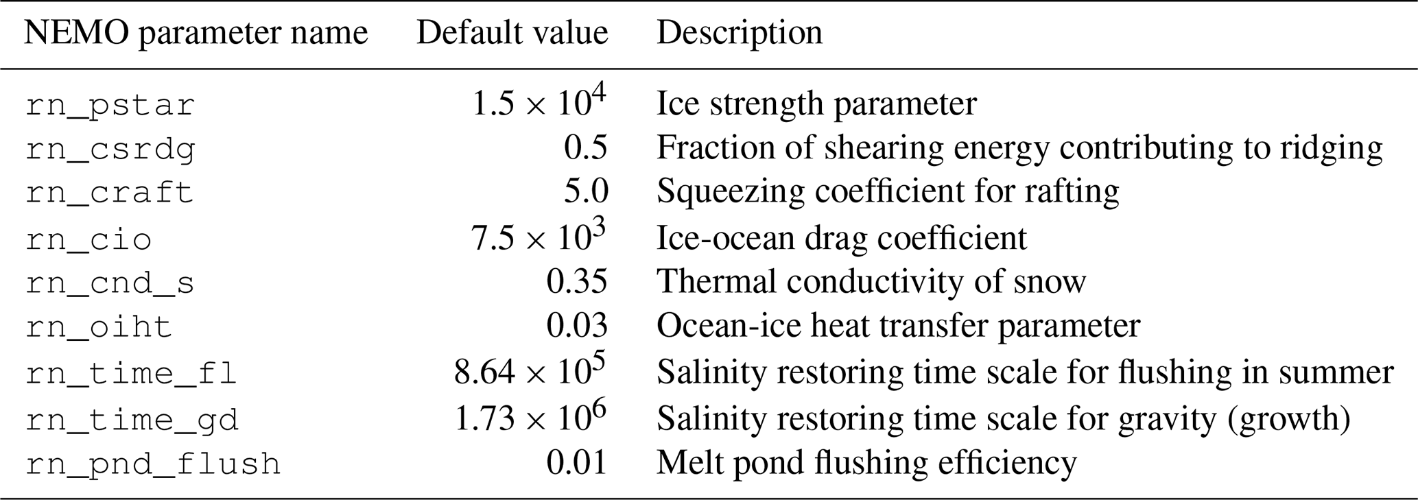
Table 1 gives a summary of which sea ice parameters are perturbed in the current implementation. The rn_pstar parameter is the same P^* parameter perturbed in Juricke et al. (2013) and follow-up work, including Strommen et al. (2022). All parameters except rn_csrdg are perturbed log-normally with σ = 0.5. The rn_csrdg parameter, which is a fraction, is perturbed using normally distributed noise by multiplying it by the value of the random noise field at that gridpoint; the perturbed value is then clipped to the range [0,1]. We also explored perturbing the prognostic albedo value, as computed by NEMO, but this was ultimately not pursued due to the large impact such perturbations had on the mean ice state. Further exploration of how to generate more moderate albedo perturbations is of clear interest, given the potential for amplifying spread further.

Table 1 Parameters being perturbed. Column 1: name of parameter in the NEMO namelist. Column 2: the default value of the parameter. Column 3: description of the parameter.

The configuration described above was determined based on a number of sensitivity tests, which tested perturbing individual parameters vs. multiple, varying σ and varying the spatial and temporal decorrelation scales. These tests suggested that each individual parameter, when perturbed, produced an enhancement in the ensemble spread with a particular spatial pattern and amplitude. Furthermore, when multiple parameters are perturbed, the resulting spatial pattern was approximately a combination of the individual patterns, with an amplitude which was higher then that achieved by only perturbing a single parameter. Examples of some of these single-parameter tests are shown in Figs. S2 and S3; note that these sensitivity tests were performed with the earlier cycle 48R2 of the IFS. This motivated our decision to perturb a large number of parameters, since this resulted in a more uniform increase in spread across the Arctic/Antarctic domain. These sensitivity tests also suggested that the parameter perturbation that has the single biggest effect is the P^* perturbation in winter and the ice-ocean drag coefficient in summer (not shown). We found little sensitivity to the spatial and temporal decorrelation scales, but a larger spatial scale generally resulted in somewhat smoother changes to spread. Varying σ scales the overall amplitude of the spread up and down as expected. These tests motivated the choice of the relatively high value of σ = 0.5, chosen in order to get an appreciable increase in spread. We comment further on this in Sect. 7.

A final comment, which may be of particular interest to anyone aiming to implement similar schemes in operational forecasts, is that when tested at a higher Tco319 resolution, there were occasional stability issues related to the build-up of sea ice at coastlines in the Arctic. These stability issues, which only appeared when the forecast was run for at least 3 months, were removed by tapering the stochastic perturbations near the coastlines, which is a feature provided by STOPACK.

4 Impact of SPP on ensemble mean and ensemble spread

4.1 Impact on the sea ice

Figure 1 shows how SPP affects the ensemble mean and ensemble spread of the seasonal mean SIC in boreal winter. The mean SIC is broadly reduced in the central Arctic, and increased around the ice edge (defined as the regions where SIC = 15 %), with the average change being a small net reduction. This results in a small increase of 0.2 % in the total sea ice area extent. More detailed analysis (not shown) suggests this change is not large enough to constitute a change in the location of the ice edge, and is rather a compactification of the existing ice edge in CTRL. We discuss the reason for this mean state change in Sect. 5.2. The ensemble spread is enhanced almost everywhere, with the greatest change (of around 1 %–2 %) seen around the ice edge, which is where virtually all the sea ice variability takes place in winter. The increased spread with SPP amounts to a relative increase of around 10 %. Figure 2 shows the equivalent impact in JJA. Here too SPP induces a net decrease of the mean SIC and an increase in ensemble spread almost everywhere. The increased spread is again roughly a 10 % relative increase. Note that we have not highlighted gridpoints where the changes in the spread are statistically significant because the vast majority of the gridpoint changes seen with SPP are significant. The same is generally true for changes to the mean, with a few notable exceptions. The increased SIC in the Chuckhi and Bering seas in DJF is not significant (p > 0.05), and in JJA the only significant changes are the larger SIC decreases of 2 %–4 % extending around the coastlines: these have been highlighted with stipling. The increased spread is significant (p < 0.05) at virtually every gridpoint for both seasons. The consistent increase in ensemble spread is expected, but the consistent decrease in the mean is not. We discuss this further in Sect. 5.1.

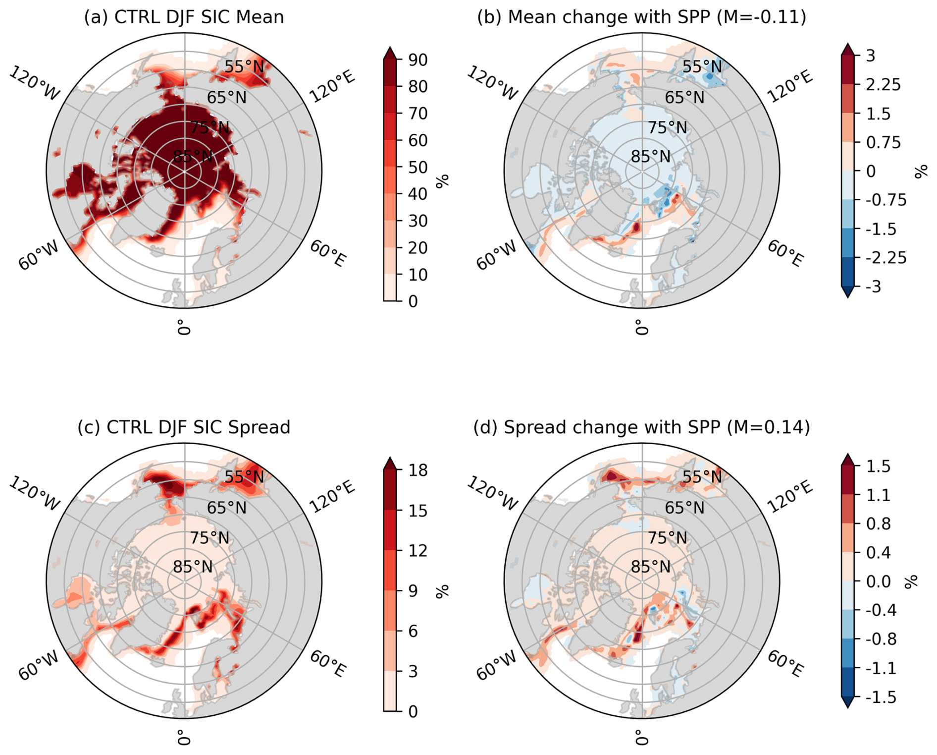
Figure 1 Impact of SPP on DJF SIC mean and spread. (a) DJF SIC ensemble mean in CTRL. (b) DJF SIC ensemble in SPP minus that of CTRL. (c, d) The same but for DJF SIC ensemble spread. The value of M where it appears is the weighted area-average across all gridpoints in the domain where SIC is non-zero.

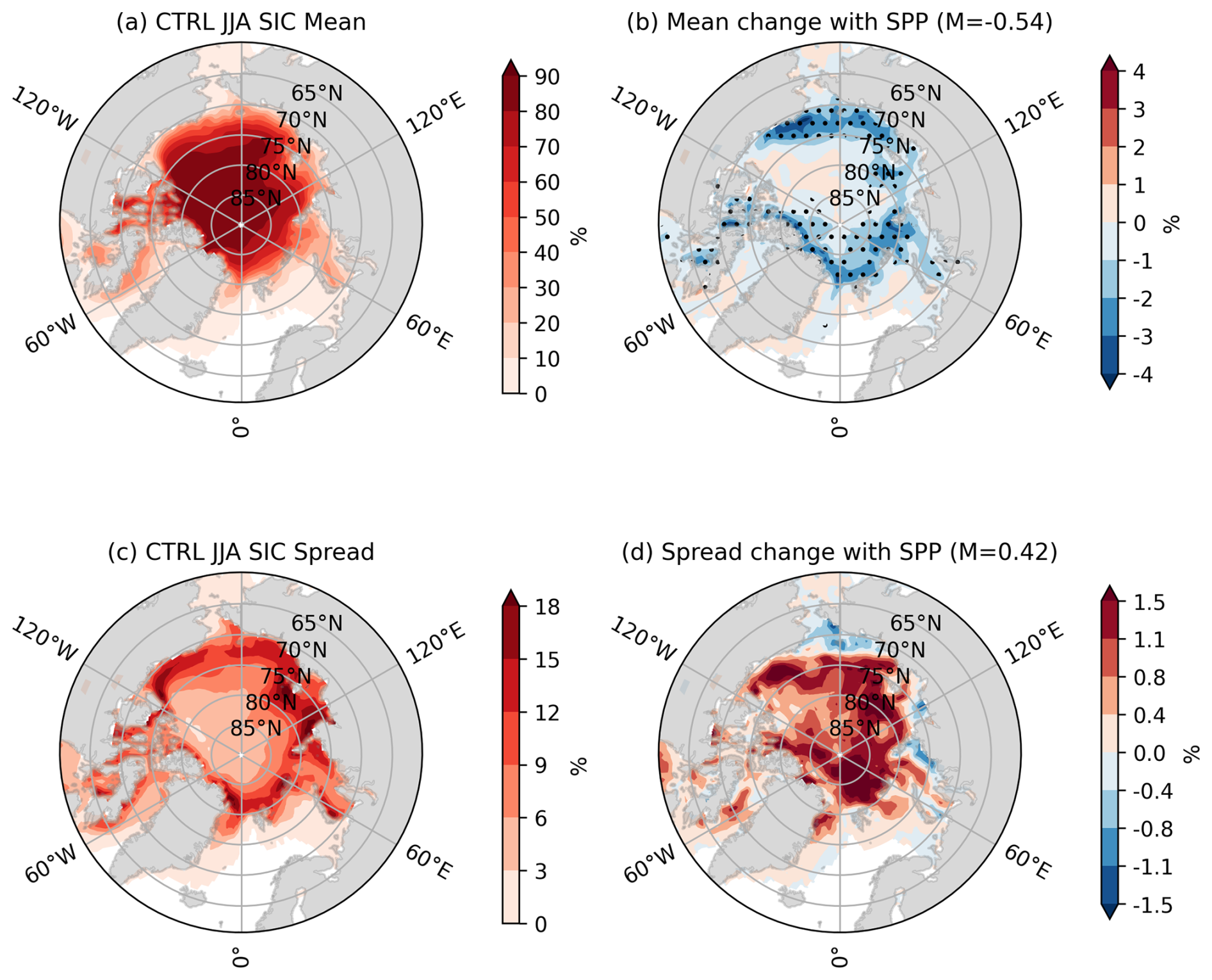
Figure 2 The same as Fig. 1 but for JJA. Stipling in panel (b) highlights where changes are statistically significant (p < 0.05).

Figures 3 and 4 show the impact of SPP on sea ice thickness. Note that thickness here means the average thickness of sea ice over the ice-covered part of the grid box. There is again a consistent increase in SIT ensemble spread, amounting to a relative increase of around 10 %. In summer there is no net change in the mean, but in winter there is a small net increase. Consistent with this, the total sea ice volume goes up by around 2 % with SPP in winter. We discuss this further in Sect. 5.2.

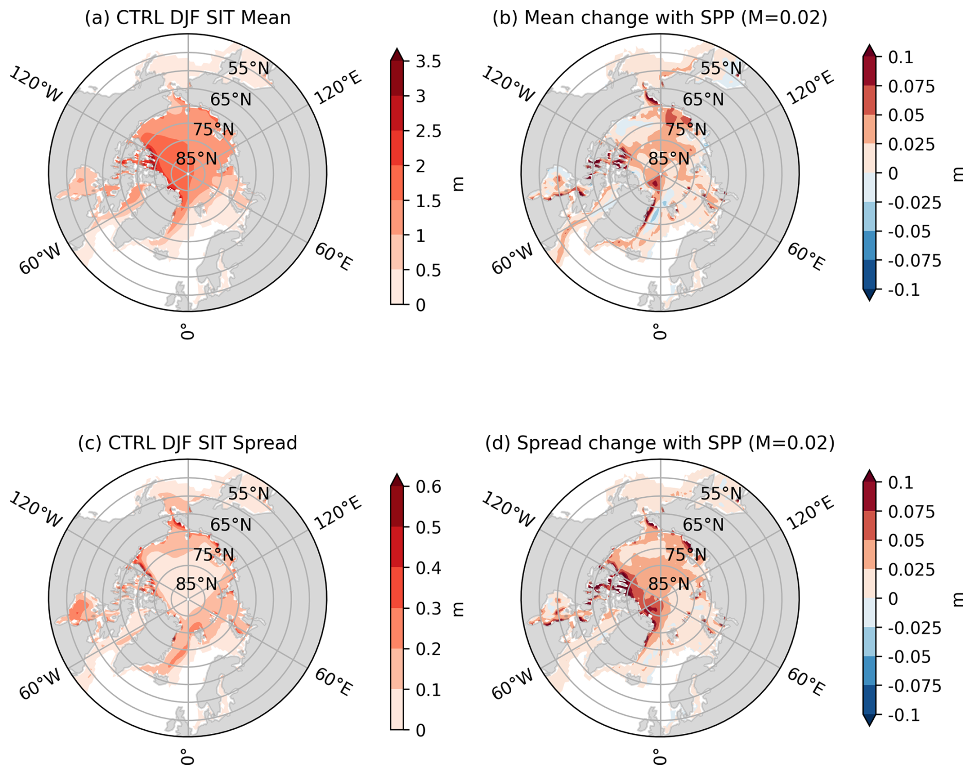
Figure 3 Impact of SPP on DJF SIT mean and spread. (a) DJF SIT ensemble mean in CTRL. (b) DJF SIT ensemble in SPP minus that of CTRL. (c, d) The same but for DJF SIT ensemble spread. The value of M where it appears is the weighted area-average across all gridpoints in the domain where SIT is non-zero.

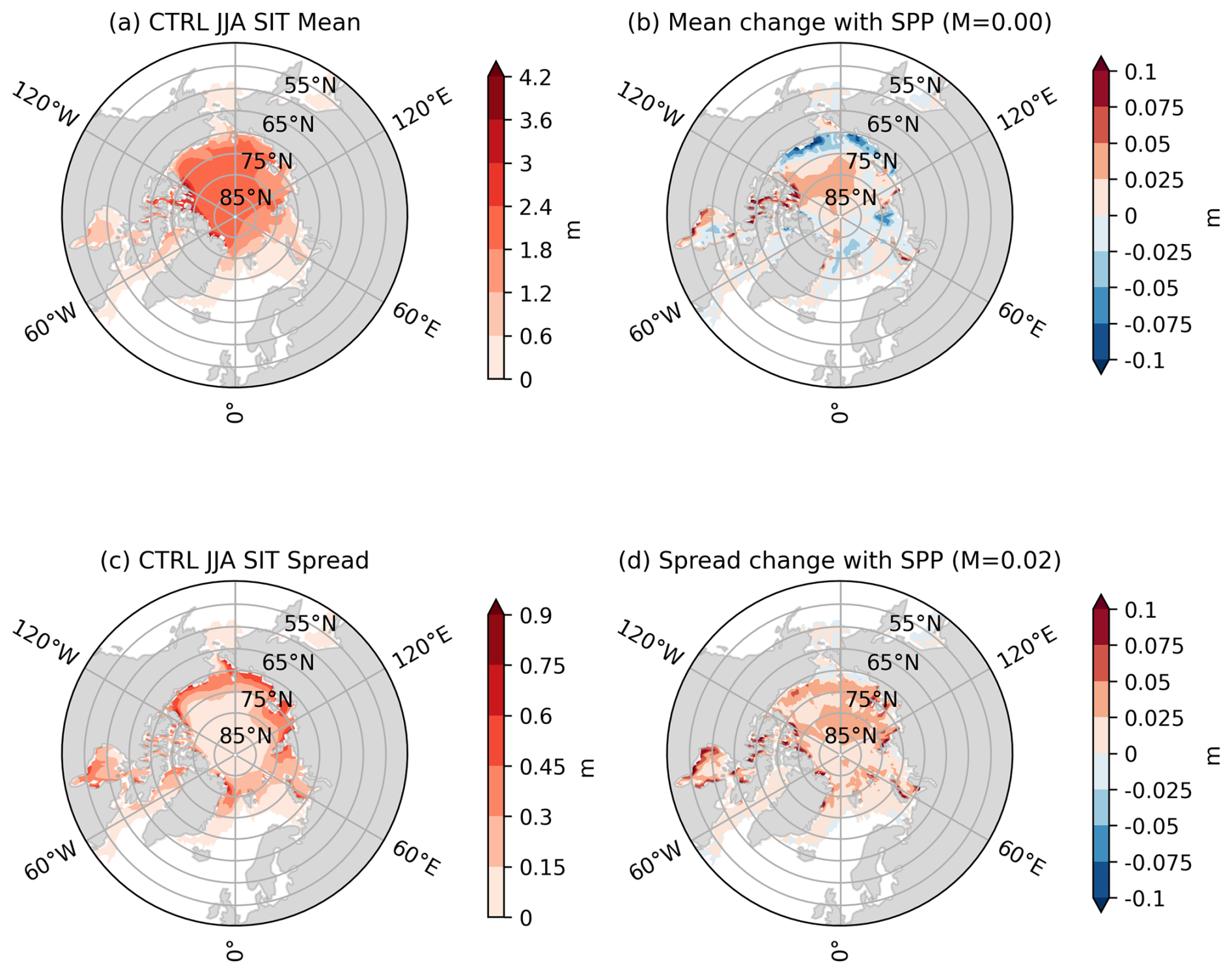
Figure 4 The same as Fig. 3 but for JJA.

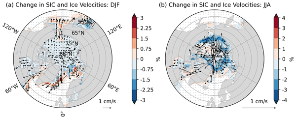
Finally, Fig. 5 shows the change in mean sea ice drift due to SPP, overlaid on the change in mean SIC. In DJF there is a clear suggestion that perturbations result in ice moving from the central Arctic to the ice edge, consistent with the changes to mean SIC. In JJA the changes in drift are far less clear, and give the impression that perturbations are resulting in random motions. The magnitude of the velocity changes are on the order of 20 % relative to the baseline velocities in CTRL. We return to this in Sect. 5.2.

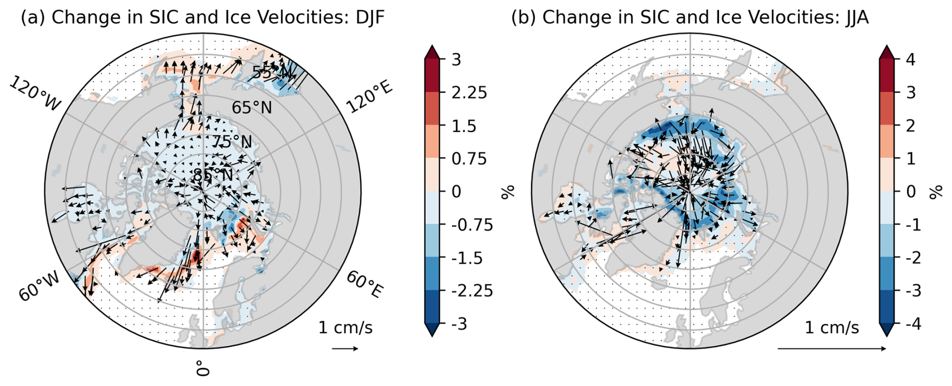
Figure 5 Impact of SPP on sea ice drift. (a) The ensemble mean change in DJF SIC with SPP (filled contour) and the ensemble mean change in sea ice velocities with SPP (black arrows). (b) The same but for JJA. The length of the arrows are proportional to the magnitude of the change. A reference arrow shows the length of a 1 cm s⁻¹ change.

4.2 Impact on the atmosphere

Figure 6 shows changes to the mean and ensemble spread of T2M and 850 hPa air temperature (T850) in winter. There is a broad warming across the central Arctic in winter, extending out to Hudson Bay, contrasted by a cooling along the ice edge of the Greenland, Barents, Kara and Chukchi seas. The direction of change is consistent at both surface and 850 hPa, though only the change around Greenland, Barents and Kara is significant at 850 hPa. A significant increase of ensemble spread is also seen in many regions of the Arctic, with a suggestion that some of the change is reaching the midlatitudes. The increased air temperature spread is an expected consequence of the increased SIC and SIT spread, as fluctuations in these quantities modulate surface heat fluxes and albedo, thereby directly altering near-surface temperatures. The changes in summer air temperature are shown in Fig. 7, and are notably smaller. This is unsurprising, since the Arctic surface air temperature in summer is tied to the freezing point and so there is little scope for the ice perturbations to affect the atmosphere. The changes to summer T2M spread appear to be closely connected to SIC and SIT changes (Figs. 2 and 4), with increased T2M spread in regions where SIC/SIT decrease with SPP and conversely.

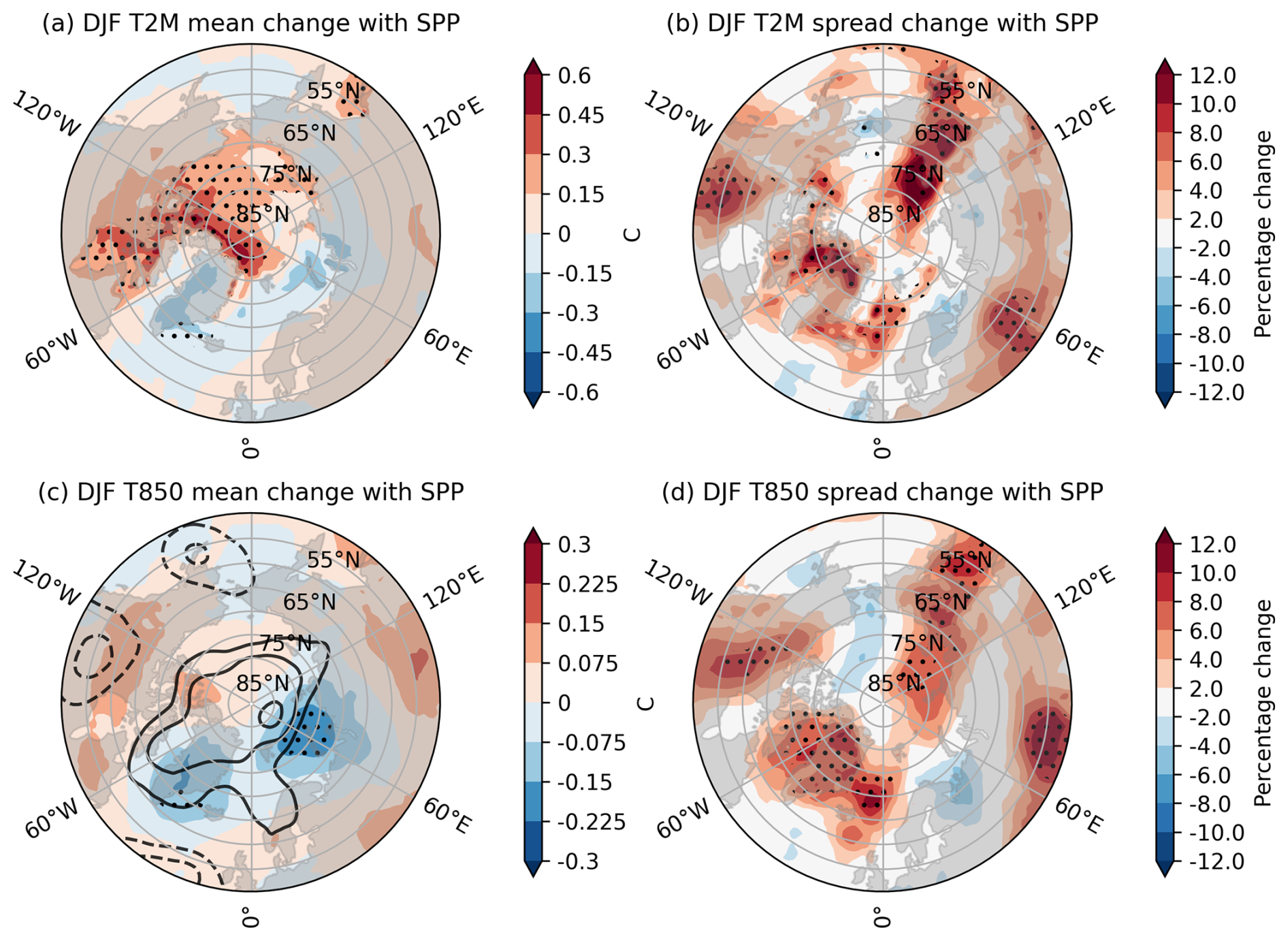
Figure 6 Impact of SPP on DJF air temperature. (a) The DJF T2M ensemble mean in SPP minus that of CTRL. (b) The change in DJF T2M ensemble spread with SPP, expressed as the percentage difference relative to CTRL. (c, d) The same but for T850. (c) The line contour shows the difference in the DJF Z500 ensemble mean, with contours drawn at ±2, ±3 and ±4 m (solid lines are positive, dashed lines are negative).

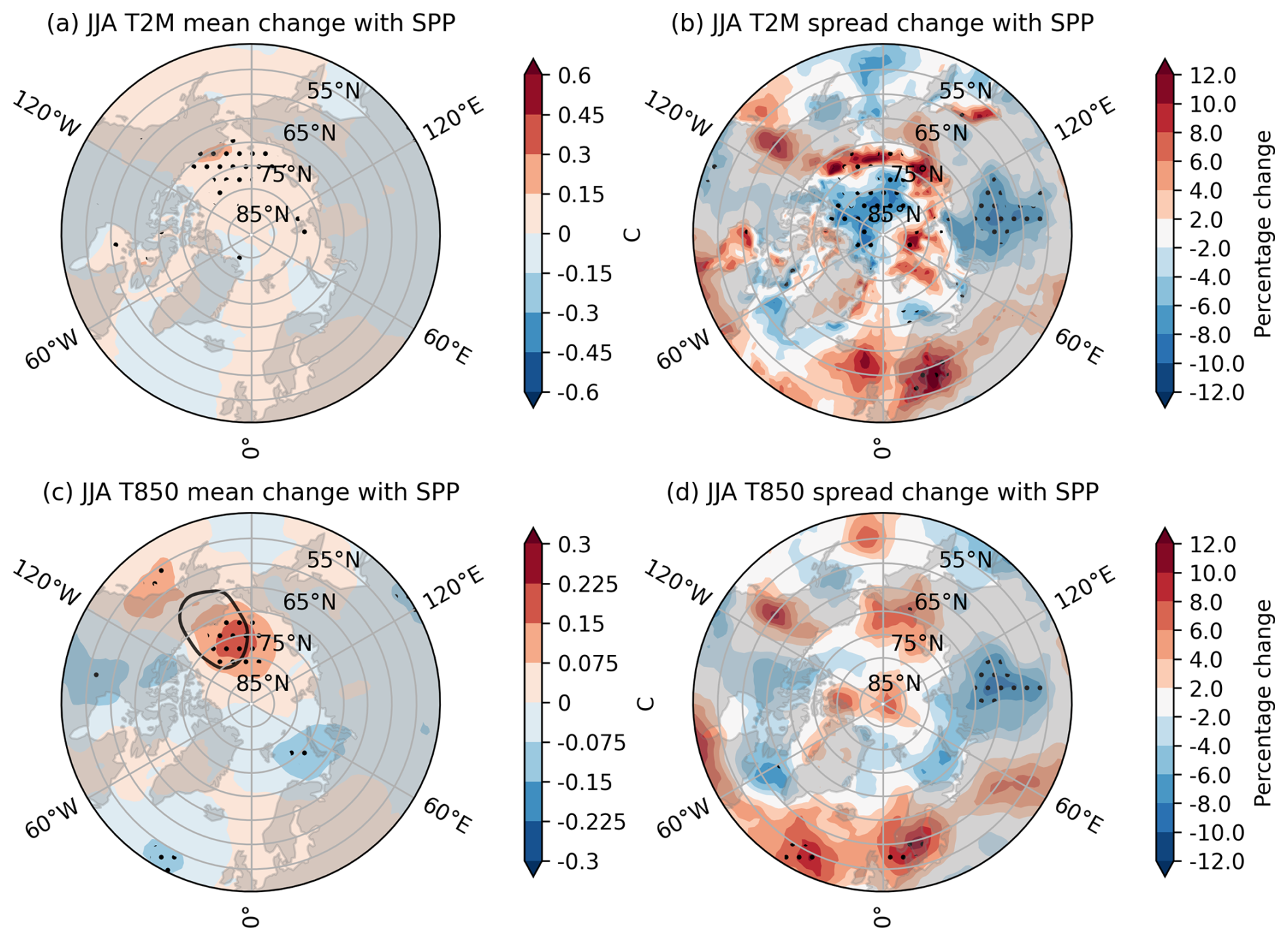
Figure 7 Impact of SPP on JJA air temperature. As Fig. 6 but for JJA. The line contours are drawn at the same levels.

In winter, the increased mean temperatures seen in the central Arctic are consistent with the reduced SIC, as this reduction allows a greater flux of heat from the warm ocean to the cold atmosphere. The decreased mean temperatures around the ice edge are consistent with the increased SIC there, for the converse reason. In summer, the changes to SIC and air temperature do not align as clearly: there is a broad decrease of SIC around the perimeter of the Arctic circle, but while the temperature goes up around the Chukchi sea, it goes down in the Barents and Kara seas. To understand these changes further we now look at circulation changes. Figures 6 and 7 also show the mean change in 500 hPa geopotential height (Z500) arising from SPP. A positive and undulating Z500 anomaly of around 2–3 m extends across most of the Arctic in winter, while in summer the Z500 anomalies are small (less than 2 m) everywhere except the Chukchi sea. To further visualise these circulation changes, we show in Fig. 8 the change in the ensemble mean 700 hPa wind vectors, overlaid onto the T850 ensemble mean change already shown. These suggest that circulation anomalies play an important role in determining the final temperature response to SPP. In particular, in winter we highlight the cyclonic anomaly centered on the Ural mountains, which results in cold Siberian air being advected over the Barents and Kara seas, consistent with the net cooling. The cooling over Greenland in winter also appears to receive a contribution from this advection. Similarly, comparatively warm marine air is advected towards the Chukchi sea in summer, consistent with the net heating there. The cooling seen over Barents-Kara in summer appears to be unrelated to circulation changes, and may rather be a result of the wintertime cooling persisting through to summer via ocean memory.

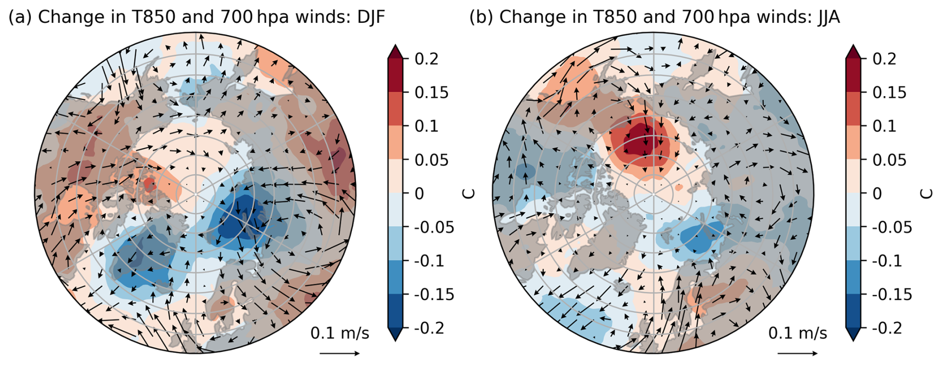
Figure 8 Impact of SPP on the circulation. (a) The change (SPP minus CTRL) in DJF mean T850 (filled contour) with the change in DJF mean 700 hPa winds overlaid as vectors. (b) The same but for JJA. The length of the wind vectors is proportional to the magnitude of the change.

To summarise, the inclusion of SPP leads to small but robust changes in the mean atmospheric circulation up to at least 850 hPa, especially in winter. In winter we also see a significant increase in air temperature ensemble spread with SPP. The mean state changes can likely be understood using the same framework as Petoukhov and Semenov (2010), namely as a combination of a local convective response, due to changes in heat fluxes, and a baroclinic response, due to changes in temperature gradients. Because the net temperature change is generally negatively correlated with the local SIC change, these effects seem to be acting coherently in our case, with the circulation changes reinforcing the local thermodynamic responses.

We emphasise here that the only difference between the CTRL and SPP experiment is the inclusion of sea ice SPP. Thus, the prime causal driver of these changes is necessarily the sea ice, not the atmosphere, even if the latter determines the final response via feedbacks. Though we note it is also possible that part of the changes to SIC are related to snow conductivity perturbations, as these could alter surface temperatures which in turn alter SIC.

4.3 Differences between coupled and uncoupled simulations

Juricke and Jung (2014) showed that the effect of sea ice perturbations on the mean ice evolution over time can differ between coupled and uncoupled simulations, which they attributed to the interactive atmosphere exerting a net negative feedback on the ice. Here we highlight that there are also large differences in how perturbations affect ensemble spread. This has implications for the use of SPP in uncoupled data assimilation which we return to in Sect. 7. To assess these differences we focus on a smaller set of 11-member ensemble forecasts, each of which is initialised on 1 January 2013 from one of the 11 unique ORAS6 initial conditions and run for 1 year. We run such forecasts using the following model configurations: coupled CTRL (no sea ice perturbations) forecast; coupled default-SPP forecast; coupled SPP forecast but using a different random field for each of the 9 perturbed parameters; uncoupled CTRL ocean-and-sea-ice-only forecast; uncoupled default-SPP ocean-and-sea-ice-only forecast. Note that here “uncoupled” means using prescribed ERA5 data as boundary forcing for a freely evolving NEMO4-SI³ simulation. Furthermore, to make the coupled forecasts more directly comparable to the uncoupled forecasts we turned off both atmospheric SPP and atmospheric initial condition spread in the coupled forecasts, so that the only source of spread comes from the sea ice SPP. We did not run an uncoupled control (i.e., without sea ice perturbations), as this would be expected to have negligible ensemble spread, due to the shared atmospheric forcing and slow timescales of the ocean and ice combined with underdispersion in the ORAS6 initial conditions. The random fields used in the simulation with independent parameter perturbations are generated using Perlin Noise, rather than the iterated Shapiro filter: see Sect. 3. The impact of these differing noise generators on changes to the SIC mean and spread were found to be minimal (not shown).

Figure 9a shows the ensemble spread for the Arctic-average SIC (40–90° N) for the various forecasts, where gridpoints with no ice are masked before averaging. In the uncoupled default SPP forecast, substantial ensemble spread is added by the perturbations (relative to the baseline spread of ≈ 0 expected without any atmospheric spread or ice perturbations), peaking in August. When changing SPP to have independent random fields for each perturbed parameter, we see a notable and consistent increase in the spread, peaking at a roughly 60 % increase in August relative to the default SPP spread. It is not a priori clear that independent perturbations should result in greater spread, as compensating effects from different physical parameters could in theory result in a net reduction in spread. However, it turns out that in this case introducing a greater number of perturbations results in much larger ensemble spread. However, in the coupled simulations the picture is far less clear. As expected, the baseline spread in the coupled CTRL is higher than in the uncoupled simulations due to the strong forcing from the atmosphere with its fast error growth, and the default SPP scheme amplifies this spread. The relative increase in spread is, however, much more modest in the coupled simulations, and there is no discernible difference between using the same random field or individual random fields.

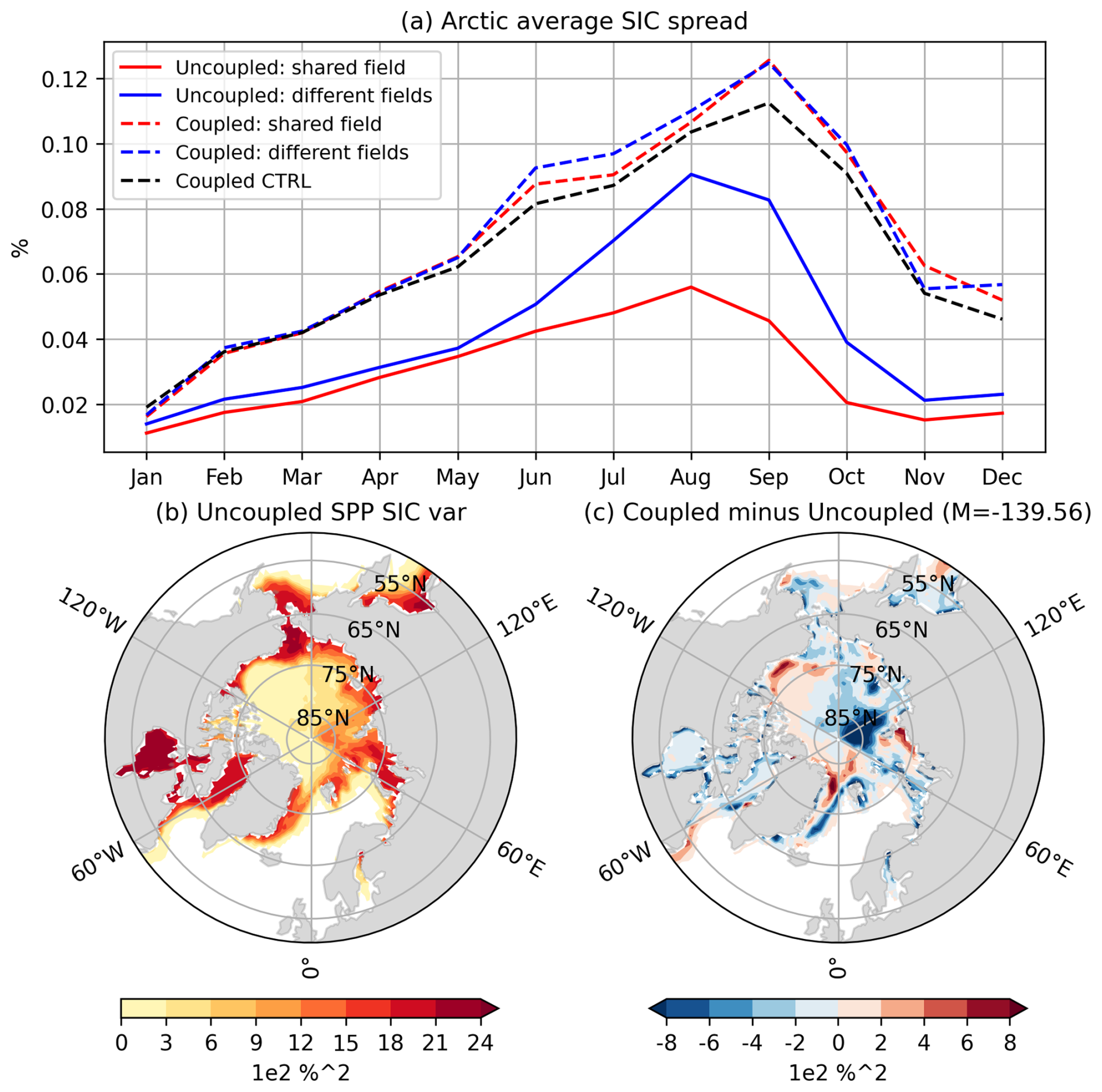
Figure 9 Impact of SPP in coupled vs. uncoupled simulations. (a) Forecast ensemble spread of the Arctic-average SIC for each month of 2013 for coupled CTRL (black dotted), coupled regular SPP (red dotted), coupled SPP with independent random fields (blue dotted), uncoupled regular SPP (red) and uncoupled SPP with independent random fields (blue). (b) The temporal variability, measured as the variance of month-to-month SIC changes at each gridpoint, for the uncoupled SPP simulation. (c) The difference in temporal variability between the coupled and uncoupled SPP simulation. For all computations, gridpoints with no ice have been masked.

These results were further confirmed using additional nudging experiments. In these experiments, coupled simulations were run in which the atmospheric vorticity, divergence and temperatures were relaxed back towards ERA5 using a 12 h relaxation time scale. They can therefore be thought of as intermediate between a fully coupled simulation and a completely uncoupled simulation. In these nudged simulations (not shown), the baseline ensemble spread of Arctic averaged SIC sits between that of the uncoupled and coupled curves in Fig. 9a: the inclusion of SPP enhances spread considerably, and switching to independent perturbations considerably amplifies this effect.

We interpret these results as saying that sea ice perturbations are far more effective at generating spread in uncoupled ocean-and-sea-ice forecasts compared to coupled atmosphere-sea-ice-ocean forecasts. We hypothesise that this is due to two effects. Firstly, in the coupled simulations the ensemble spread is dominated by the atmospheric spread, meaning that ice perturbations will, relatively speaking, be less effective at amplifying spread compared to uncoupled simulations where ensemble spread is purely ice driven. In fact, the ensemble spread may be close to saturated in the coupled simulations. We computed that the ensemble spread for the coupled CTRL in August is approximately the same as the standard deviation of detrended interannual variations in August. If it is assumed that the variation in monthly sea ice from one year to the next is an approximate upper bound on how much the sea ice is capable of changing within a single month, then this suggests that the spread may already be close to the maximum of what is achievable given the inherent timescales of the ice. Further increases to spread are likely to be difficult to achieve as a result. Secondly, as suggested in Juricke and Jung (2014), the atmosphere may be acting to damp the SPP-induced ice anomalies via negative feedbacks.

These two hypothetical effects can be qualitatively supported using idealized models of the coupled ice-atmosphere system based on stochastic differential equations: see, e.g., Strommen et al. (2022). We refer to such an idealized model as a “LIM”, short for “linear inverse model”, following typical conventions: see Text S1 in the Supplement for details. One can show that (a) coupled LIM simulations with a negative atmospheric feedback show greater overall ensemble spread compared to corresponding uncoupled LIM simulations, but that (b) increased stochastic forcing is much more effective at increasing ensemble spread in uncoupled LIM simulations: see Text S1 and Fig. S4. Both the negative feedback and the dominance of atmospheric forcing contribute to this effect in the LIM, though the latter effect seems to be more important in the range of parameter values we considered. It is challenging to quantitatively estimate the sign of the atmospheric feedback in NWP models, because the net feedback is a combination of both immediate local thermodynamic feedbacks and slower timescale dynamical adjustments which can originate further afield. However, in the LIM, the clearest signature of a negative atmospheric feedback is reduced temporal variability in coupled vs. uncoupled simulations. In Fig. 9b we show the month-to-month SIC variability across all ensemble members for the uncoupled SPP forecast, and in (c) we show how this temporal variability differs in the coupled SPP forecast. The sign is broadly negative, consistent with the atmosphere exerting a net negative feedback.

5 Mechanisms underlying the impact of SPP

In Sect. 4 we have seen that SPP alters the mean and spread of SIC and SIT in a particular way. The aim of this section is to shed light on why we see these particular impacts. In Sect. 5.1, we show that changes to the ensemble mean and ensemble spread are strongly related, and in Sect. 5.2 we present a simple conceptual model which explains many of the observed features.

5.1 How are changes to the sea ice mean and spread related?

Figures 1 and 5 show a consistent picture of SPP resulting in ice being advected outwards with associated changes to the mean. This suggests the stochastic perturbations may be at least partially exerting a consistent change to the system despite being random and mean zero. Furthermore, such systematic changes to the mean may not be independent of the changes to the ensemble spread, due to the strong asymmetries present in the sea ice. In this section we aim to shed further light on how the mean state, mean state changes and ensemble spread changes are related, where changes are always understood as changes due to SPP.

Figure 10a and b show scatter plots of seasonally averaged SIC mean state changes vs. ensemble spread changes at each gridpoint in the Arctic for winter and summer. Thus, for DJF, we take the values at each gridpoint in Fig. 1b as the x coordinates and the values in Fig. 1d at the corresponding gridpoints as the y coordinates. To give a clearer sense of where most of the points are actually located, we also estimated the 2D probability density function (pdf) using a kernel density estimator with Gaussian kernels. The 90th percentile of this estimate is shown as a red contour.

In winter, while most points experience a small reduction in mean SIC and a small increase in the spread (red contour), there is clear evidence of non-Gaussian structure in the point cloud. In summer, the majority of points show the same clear tendency for reduced mean and enhanced spread (red contour), but the long tail of points in the upper right quadrant is absent. We can understand the non-Gaussian features by highlighting points where the baseline CTRL mean SIC is high (SIC > 80 %) and low (SIC < 20 %): see Fig. 10c–f. Here the red contour again shows the 90th percentile of the estimated pdf, but this time estimated only on the subset of points being considered (i.e., the mauve points in the middle row and the blue points in the bottom row). It can be seen that these two categories of ice, the ice pack on the one hand and the ice edge zone on the other, occupy distinct “regimes” as far as impacts of SPP go. In the ice pack regime, there is a visually clear negative correlation between changes to the mean and the spread: points where the mean go down more experience a greater increase in spread. The linear correlation ranges between −0.5 and −0.7 in the two seasons (p < 0.05). On the other hand, in the ice edge zone the correlation is positive: points where the mean goes up more experience a greater increase in spread. The linear correlation is smaller in this case, ranging between 0.3 to 0.4 in the two seasons (p < 0.05).

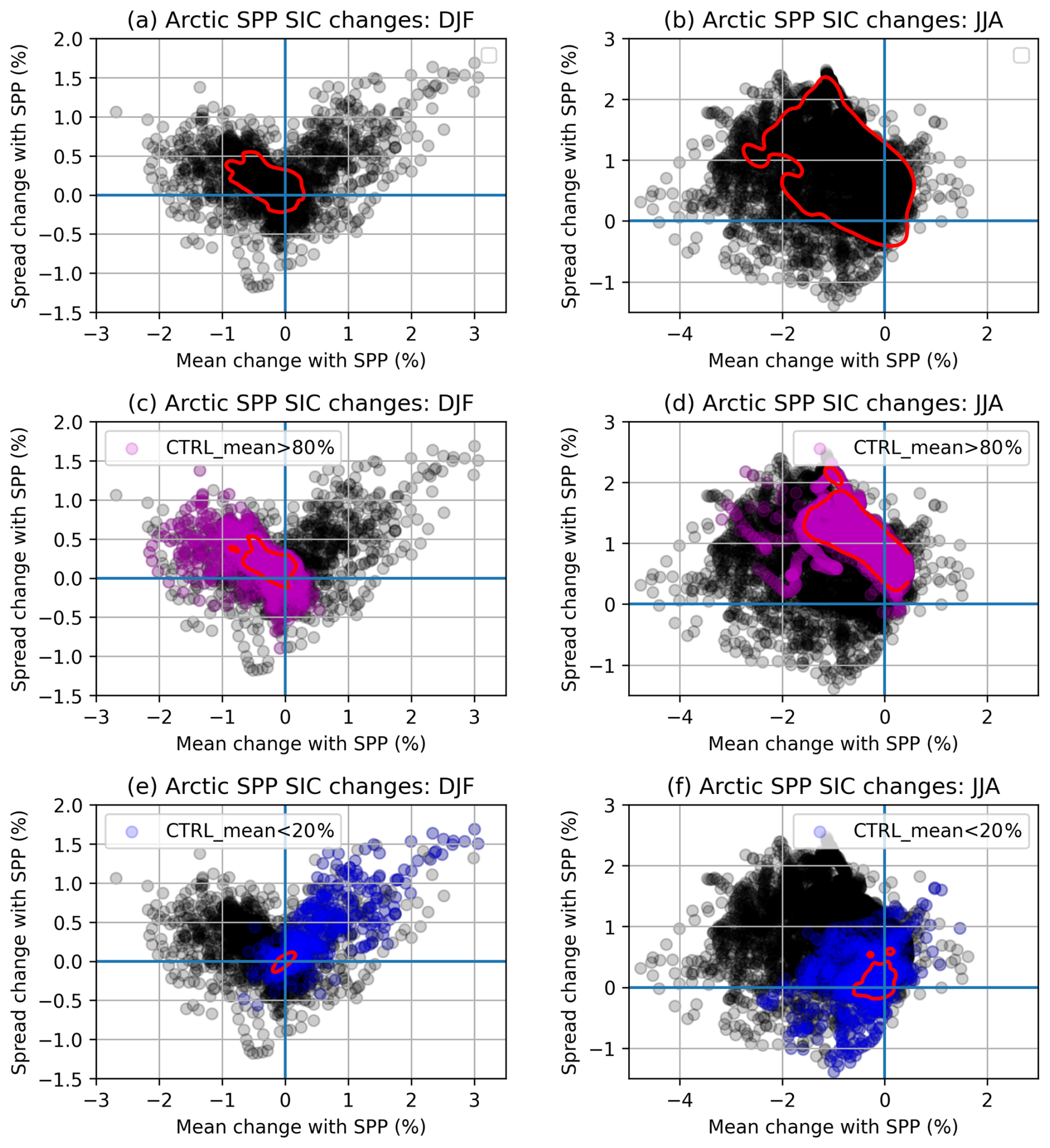
Figure 10 Relationship between changes to the mean and the spread. (a) Scatter plot of the SIC ensemble mean change vs. the ensemble spread change at each gridpoint in the Arctic (60–90° N) for DJF averages. The red contour encloses 90 % of all the points. (c, d) The same as (a) and (b) but gridpoints where the CTRL ensemble mean SIC exceeds 80 % are marked in mauve. (e, f) The same as (a) and (b) but gridpoints where the CTRL ensemble mean SIC is less than 20 % are marked in blue.

The spatial asymmetry of the changes in winter (decreased SIC in the ice pack and increased SIC at the ice edge) suggests that some of the relationships highlighted above may be related to how the impact of perturbations differs depending on the underlying mean SIC state in the CTRL experiment. To assess how changes to the SIC mean and spread depend on the CTRL mean state, we show in Fig. 11 2D histograms of these quantities, normalised so each column sums to 1. This normalisation is for visual clarity: the raw histograms are bimodal, especially in winter, being dominated by gridpoints that are close to 100 % SIC or close to 0 %. The normalisation makes it easier to assess changes in the less common intermediate values. From this figure we can see that in winter, the mean SIC tends to increase in regions where the initial SIC mean is low (< 10 %), and to decrease in all other regions. The decrease is especially large in regions where the initial SIC is close to 100 %. The spread is broadly enhanced independently of the initial SIC mean. This is consistent with the impression of Fig. 1, since the gridpoints where the initial SIC is low in winter are precisely those along the ice edge, and the gridpoints where the initial SIC is high are those in the central ice pack. In summer the patterns are less clear. Spread increases almost everywhere, while the mean only increases in regions where the initial SIC mean is very low or very high, and decreases otherwise. Again, this is consistent with Fig. 2, which shows changes that are not immediately obviously related to the baseline CTRL mean. We note that the picture is largely the same in the Antarctic (not shown).

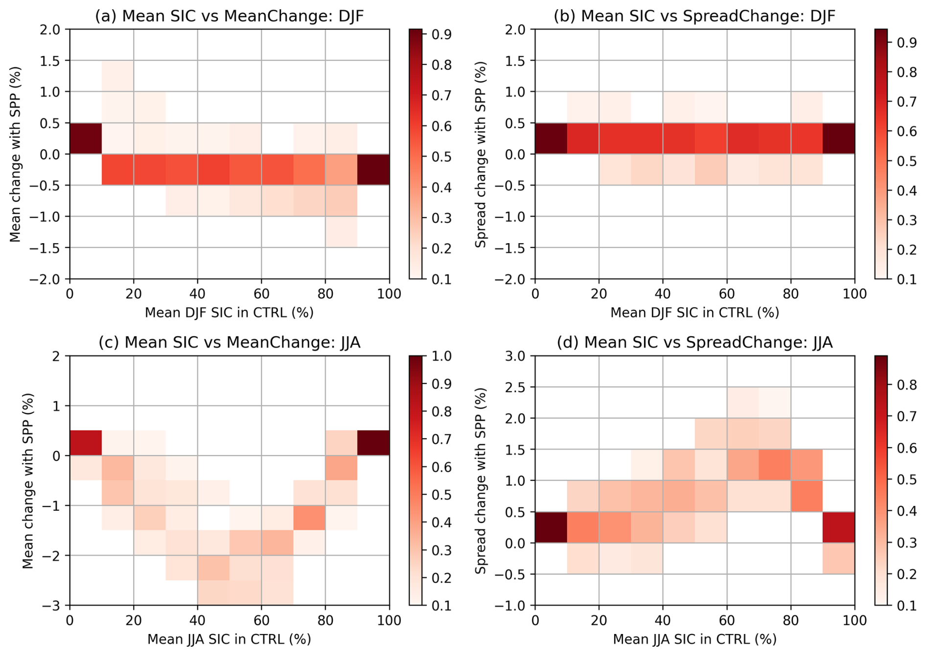
Figure 11 Dependence on the basic mean state. (a) 2D histogram of the mean DJF SIC in CTRL against the mean SIC change with SPP at each gridpoint in the Arctic (60–90° N). For visual clarity each column has been normalised to sum to 1. (b) The same but showing mean DJF SIC in CTRL against the spread change with SPP. (c, d) Equivalent histograms for JJA.

To summarise, changes to the mean sea ice and changes to the sea ice ensemble spread are not independent of each other, and there is clear evidence of distinct regimes within which the covariance of these two changes is strongly constrained. In the next section we discuss the likely reason for this.

5.2 Conceptual model of the impact of SPP

It is natural to speculate that many of the impacts of SPP, including the impact on the mean SIC and the relationship between the mean and spread, can be explained by the strong asymmetries and non-linearities present when perturbing sea ice. Some of these asymmetries exist at the level of the parameters themselves. For example, Juricke et al. (2013) argued that low values of P^* (rn_pstar in Table 1) are more effective at reducing the ice strength than high values are at increasing it, meaning that mean zero perturbations to this parameter can systematically push the system towards weaker ice. This in turn can promote enhanced drift (e.g., from the ice pack to the edge in winter) and break-up of ice. Because we perturb 9 parameters which all interact with each other, understanding such parameter-level asymmetries in detail is not feasible. However, we argue that a simple conceptual model based on more fundamental asymmetries already has good explanatory power. Concretely, we present a conceptual model which aims to explain three broad features: (1) the overall reduction in the mean SIC, (2) the changes to sea ice drift in Fig. 5, and (3) the broad dependences between the mean and the spread discussed in the previous section. It does this by considering two fundamental asymmetries: a distributional asymmetry owing to SIC being bounded above and below, and a spatial asymmetry arising from ice advection: in regions where SIC is close to 100 %, convergence will tend to be counteracted by internal ice forces, whereas this is not the case in regions with some open water. When explaining this model, we assume that we are dealing with DJF for simplicity, and then explain afterwards how the picture changes in JJA.

The first asymmetry comes from the fact that SIC is bounded above and below. Thus, if one perturbs a gridpoint which is close to 100 % SIC, one will only see an effect if the perturbation is acting to decrease the SIC. Furthermore, the SPP scheme only perturbs gridpoints where there is some sea ice. Thus, if a perturbation pushes a gridpoint with very low SIC down to zero SIC, that gridpoint will in effect become invisible to SPP. In particular, SPP will not be able to re-freeze the water at that gridpoint in and of itself. Because the distribution of SIC is strongly bimodal (Fig. 12a), these two boundary cases actually represent the majority of cases. This suggests the perturbations will tend to decrease the SIC. This suggestion can be confirmed in a simplified statistical model. We start by drawing a sample from a strongly bimodal distribution with peaks close to 0 and 100, which is then clipped to be bounded by 0 and 100. We then “perturb” this distribution by adding random white noise with a specified standard deviation to the samples: samples that end up below zero are removed, while samples that end up above 100 are clipped to 100. Iterating this 100 times for multiple choices of standard deviation results in Fig. 12b, which confirms that this procedure produces a consistent decrease in the mean which scales with the magnitude of the perturbations. The effect is stronger the more perturbations are applied (not shown). We emphasise that this is purely a toy-model and the specific numbers in the figure are not meant to be taken at face value. In particular, the complete removal of samples going below zero is likely too strong an assumption, because if spurious melting occurs in SI³ due to a perturbation the model will typically push towards forming new ice at the next time step. We also note that because SPP perturbs sea ice parameters and not the sea ice itself, it is hard to know how to best construct such toy-models; e.g., is the net effect of SPP on the SIC tendencies themselves actually white noise? But Fig. 12 at least supports the basic heuristic. The same heuristic also implies that gridpoints where the SIC is very low will tend to show a net increase with perturbations, and the gridpoints with very high SIC will show a clear decrease. This is what was seen in Fig. 11a.

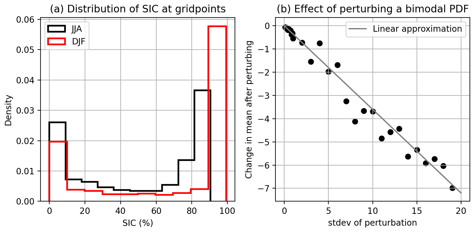
Figure 12 Toy-model for SPP's mean state impact. (a) Histograms of the DJF (red) and JJA (black) SIC at all Arctic gridpoints in the CTRL model. (b) Change in the mean of a truncated bimodal distribution when repeatedly applying white noise with a given standard deviation, as a function of this standard deviation. The grey line is a linear fit to the points.

This first distributional asymmetry can also explain the relationships found in the previous section between the original mean state, mean state changes and ensemble spread changes. When gridpoints close to 100 % SIC experience a reduction in SIC due to SPP, the variability will also increase, because points where the ice is particularly dense are constrained from moving or changing. We therefore expect a negative correlation between mean state changes and ensemble spread changes across such gridpoints. On the other hand, for gridpoints close to 0 % SIC the opposite occurs: increasing the SIC is now expected to enhance spread, as there is more ice to move around, while reducing it can bring the spread down to zero by removing it entirely. We therefore expect a positive correlation for such gridpoints. This positive correlation may be further enhanced by thermodynamic effects: if the SIC is increased at a gridpoint with low initial SIC, the cold atmospheric temperatures may act as a positive feedback. These expectations are realised in Fig. 10.

The second fundamental asymmetry is the spatial asymmetry between regions with close to 100 % SIC and regions with less than 100 %. In winter this is the asymmetry between the ice pack and the marginal ice zone. When the perturbations affect ice advection in winter, moving the ice towards the central Arctic requires sufficient energy to cause ice to pile up. On the other hand, there is little resistance against moving the ice towards the edge. Thus given random changes to the advection of ice, we should expect to see a net movement towards the ice edge, as this is the path of least resistance. This is exactly what is seen in Fig. 5a.

This conceptual model therefore explains the basics of how SPP alters SIC in winter. How applicable is to summer? Note that while there are no gridpoints with close to 100 % SIC in summer (the maximum attained by CTRL in JJA in the Arctic is 90 %), the distribution is still highly bimodal: see Fig. 12a. Thus the first distributional asymmetry still suggests that perturbations should decrease the mean on average. The main difference is that there is now scope for perturbations to push the highest SIC values even higher (i.e., from the 80 %–90 % range to the 90+ % range). Indeed, this is what is seen to occur in Fig. 11c, in contrast to winter. The other difference is that there is less scope for a positive thermodynamic feedback when the SIC is increased at a gridpoint with a low initial SIC. This likely explains the difference between panels (a) and (b) in Fig. 10 in the upper right quadrant.

Regarding the spatial asymmetry, it is also still the case that when ice advection is perturbed randomly, the path of least resistance is away from the regions of maximum SIC. In JJA, this is the region north of Canada, extending towards the central Arctic. Thus one might expect the perturbations to induce random motions around, but not into, this region. Figure 5b suggests this does happen to some extent, though the picture is far less clear than in winter. This perhaps suggests that weaker summer ice allows perturbations to more easily induce convergence into high SIC regions. Nevertheless, the conceptual model can still explain several of the features in summer.

In summary, these asymmetries, and the purely statistical or mechanical consequences of them, already likely explain much of the SIC mean state change seen with SPP, including the increased sea ice extent in winter. These results are also found to be largely similar in equivalent experiments run at higher atmospheric resolution and in simulations where independent perturbations are applied to each parameter (not shown). We have so far only discussed SIC, but we believe the increase in the mean SIT is also related to a distributional asymmetry: SIT is bounded below but not above, and hence random perturbations will tend to push the SIT towards higher values. An asymmetric impact associated with irreversible processes such as ridging is also a likely explanation for the increase in SIT in regions where ice typically converges. This could also explain the increase in sea ice volume with SPP.

We stress that this conceptual model cannot explain all the observed features, such as the detailed spatial variations in Figs. 1 and 2, or the full shape of the histograms in Fig. 11. Such detail would likely require understanding the effect of individual parameters, which we do not pursue here. Another important caveat is that Juricke and Jung (2014) showed that the response to perturbations can undergo distinct phases, with an initial multidecadal transient phase in which the system equilibrates with the perturbations, after which the response can then differ. The changes seen in our simulations thus only show the very initial part of the transient response, which is nevertheless the part relevant for weather as well as sub-seasonal and seasonal predictions. It is possible that our conceptual model is only informative for this phase, with slower timescale and harder to predict physical feedbacks dominating the longer response.

6 Impact on seasonal forecast skill

6.1 Impact on sea ice forecast skill

We have seen that SPP changes both the ensemble mean and ensemble spread of the SIC forecast. We now examine how this impacts forecast skill, focusing on SIC. Figure 13 shows how SPP changes the RMSE, spread-error ratio and CRPS for seasonally averaged winter SIC, where we remind the reader that the DJF-mean bias has been removed before computing the metrics. The change in RMSE is slightly negative on average (i.e., the error goes down), a result of broad improvements in the central Arctic averaged against more mixed impacts at the ice edge. For the spread-error ratio minus 1, there are large negative values in CTRL, confirming the underdispersion of SIC forecasts in the IFS (spread-error ratio smaller than 1). The main exception is the Chukchi Sea and near Iceland, where overdispersion occurs. Adding SPP enhances spread and hence brings the ratio closer to 1 almost everywhere, though only by a small amount relative to the CTRL bias. The exception is again at the ice edge near Iceland and the Chukchi Sea, where the overdispersion in CTRL is often amplified. The increased spread-error ratios manifest already within the first forecast month and are consistent thereafter (not shown). For CRPS, the improved spread results in broadly better (i.e., lower) scores, though some important exceptions exist at the ice edge, especially in the Greenland Sea.

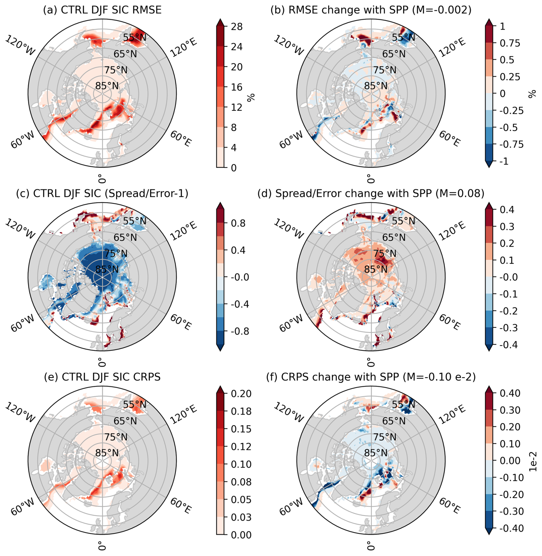
Figure 13 Impact of SPP on winter SIC forecast skill for months 2–4. (a) The RMSE of DJF SIC for the CTRL forecast. (b) The difference in RMSE with SPP. (c, d) The same but for the spread-error ratio minus 1 (so a value of 0 means perfectly calibrated). (e, f) The same but for the CRPS of the bias corrected forecasts. The values of M in the titles are the area-weighted mean across all gridpoints where the SIC is non-zero. Forecasts are validated against OSI-SAF.

This mixed impact is likely related to how SPP changes the mean bias. Even though the SIC forecasts have been bias corrected to have no bias on average across the period 1993–2023, there are still many individual forecasts where both CTRL and SPP predict non-zero SIC values at gridpoints where no sea ice exists in observations. In such cases the forecast is heavily penalised. In other words, the binary nature of sea ice means that the typical bias correction approach cannot remove all the effects of model biases. This explains why the CRPS is worse with SPP in the Greeenland sea: SPP slightly increases the bias there resulting in greater penalties at gridpoints where no sea ice was present in observations. Similar reasoning explains the negative impact of SPP for RMSE and the spread-error ratio. It is plausible that the use of calibration methods more tailored to sea ice, such as those discussed in Dirkson et al. (2022), would reveal a more positive improvement due to SPP.

In summer (Fig. 14), spread-error ratios are almost uniformly improved, although as in winter the magnitude of the change is small. Changes to RMSE and CRPS are less clear cut, consistent with the more spatially varying changes to the mean SIC seen in Fig. 2.

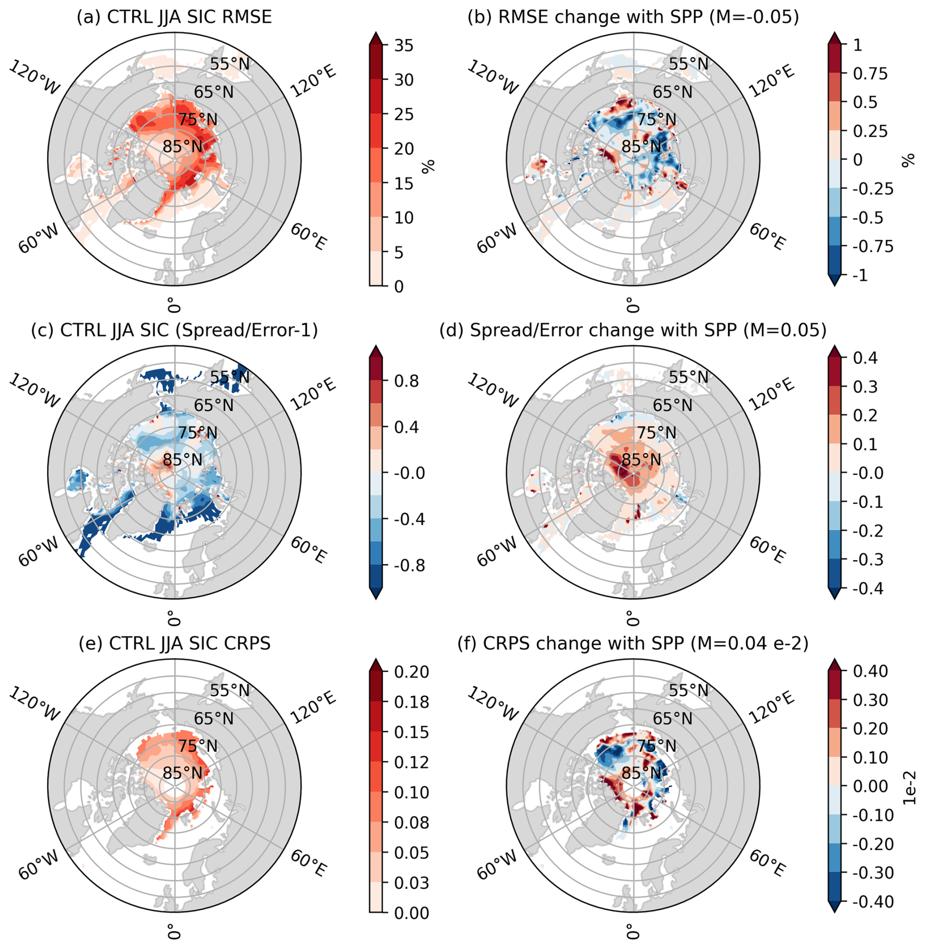
Figure 14 Impact of SPP on summer SIC forecast skill for months 2–4. As Fig. 13 but for JJA.

6.2 Impact on atmospheric forecast skill

We have already seen in Sect. 4.2 that the SPP-induced changes to the sea ice affect the atmosphere. We now examine how these changes affect forecast skill. We restrict attention here to winter only, because SPP has a very limited impact on the atmospheric mean state in summer (Fig. 7). While it is possible that more extreme Arctic sea ice events could have a larger impact on the atmosphere in summer (Balmaseda et al., 2010; Petrie et al., 2015), assessing this goes beyond the scope of the present work. We also restrict the discussion to T850 and Z500, thus avoiding T2M, where validation in the Arctic is highly uncertain (Tian et al., 2024).

Figure 15 shows the impact on T850 RMSE, spread-error ratios and bias-corrected CRPS. There is a decrease in the RMSE along the Greenland, Barents and Kara seas, which is consistent with a robust reduction in the mean bias here arising from the SPP induced mean change (see Figs. 6c and S5). Changes elsewhere are also consistent with changes to the mean bias (Fig. S5) but these are less clearly related to robust shifts in the ice so may reflect noise. The spread-error ratios are also increased around Greenland and the Kara sea, but in the former case this is a small degradation. Given these mixed impacts on RMSE and spread-error ratios, it is not surprising there is little change to the CRPS of bias-corrected fields.

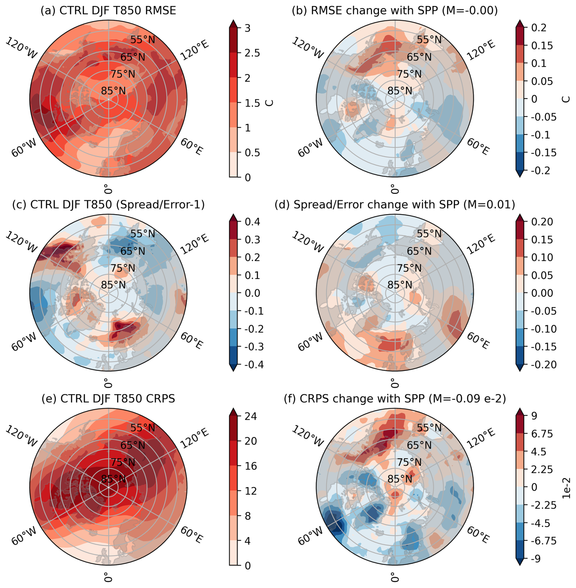
Figure 15 Impact of SPP on winter T850 forecast skill for months 2–4. (a) The RMSE of DJF T850 for the CTRL forecast. (b) The change in RMSE with SPP. (c, d) The same but for the spread-error ratio minus 1 (so a value of 0 means perfectly calibrated). (e, f) The same but for the CRPS of the bias corrected forecasts. The values of M in the titles are the area-weighted mean across all gridpoints. Forecasts are validated against ERA5.

Given the potential for stochastic sea ice perturbations to influence the midlatitude circulation via Arctic-midlatitude links (Strommen et al., 2022), it is of interest to assess changes in Z500 skill with SPP. Consistent with other seasonal forecast studies, we use the ACC as our measure of Z500 skill (Johnson et al., 2019). We emphasise that for Z500 at these lead-times, the ensemble mean Z500 amplitudes are typically much smaller than those that actually occur, and hence the RMSE of the Z500 forecasts are generally very high, even in cases where the ACC is high. Thus high ACC should be understood simply as consistent phase agreement.

Figure 16a shows the change in ACC with SPP in winter. There is a large increase in the sub-polar North Atlantic, extending into Scandinavia, with the difference peaking at around 0.5. The differences are found to be statistically significant at many gridpoints. Note that since consecutive Z500 samples are separated in time by a full year, the autocorrelation is close to zero at each gridpoint for CTRL, SPP and ERA5. Thus, estimates of significance are unlikely to be related to the presence of, or changes to, serial correlation. However, it must be highlighted that the sample size of 30 is small, with 40 or more samples typically being necessary for the test to have sufficiently high power in this context (Siegert et al., 2017). More importantly, when applying either of the two tests we used to account for a multiple-testing fallacy (see Sect. 2.2), we found that field significance is not achieved. Concretely, we estimate that the probability of obtaining, by chance, the same number of significant gridpoints as in Fig. 16a, is around 40 %. The probability of obtaining, by chance, spatially coherent patches of significant gridpoints comparable in area to those in Fig. 16a was estimated to be similar. The apparent ACC changes with SPP must therefore be treated extremely cautiously, and may be random, despite the large amplitude of the change and gridpoint-level significance. However, a similar increase in ACC in the North Atlantic region was found in several other seasonal hindcasts using SPP with slightly different configurations (e.g., different atmospheric resolution or a different random noise generator; not shown). This region also aligns with where SPP has robustly changed the sea ice mean and variance, and there is a broad model consensus that sea ice can affect mid latitude Z500 (Smith et al., 2022). We therefore believe it is reasonable to consider the possibility that the signal is real, which we assume to be the case in what follows.

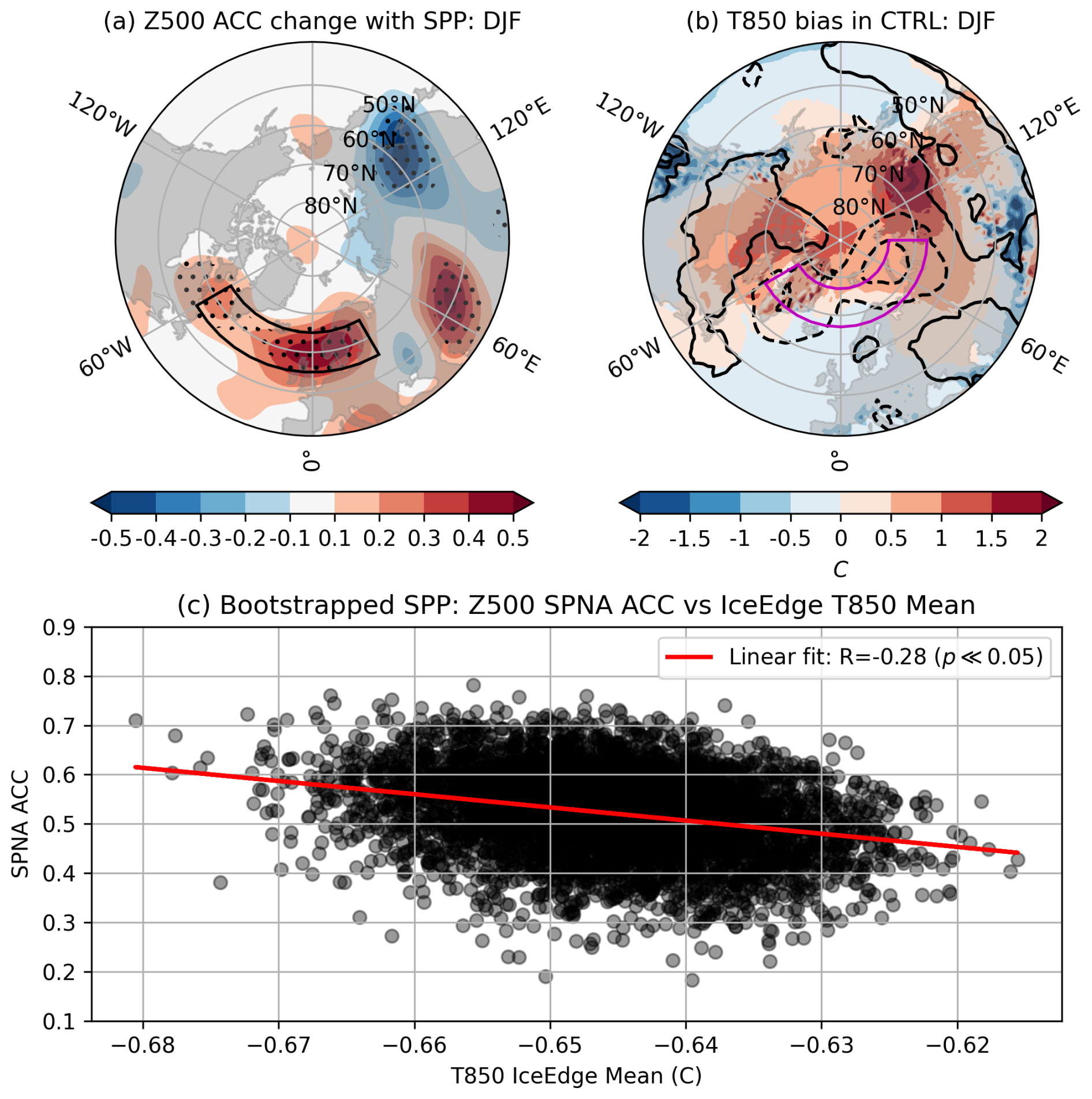
Figure 16 Impact of SPP on winter Z500 forecast skill for months 2–4. (a) Difference in DJF Z500 ACC between SPP and CTRL at every gridpoint. The black box highlights the SPNA region. Stipling denotes significance (p < 0.05). (b) The DJF T850 bias in CTRL (filled contour) and the change in the T850 ensemble mean with SPP (line contours; marked at ±0.05, ±0.15, ±0.25 °C; solid lines are positive, dashed lines are negative). The mauve box highlights the IceEdge region. (c) Scatter plot of SPNA ACC's vs. the mean T850 in the IceEdge region, obtained by bootstrap resampling the SPP ensemble with replacement 5000 times. The red line is the linear fit. Forecasts are validated against ERA5.

If we define a broad sub-polar North Atlantic (SPNA) box by 55–65° N, 60–30° W (black box in the figure), then the ACC of SPNA-averaged Z500 increases from around 0.3 in CTRL to 0.6 with SPP. The spatial pattern of the skill increase only partially overlaps the NAO pattern, and the DJF NAO forecasts in SPP therefore exhibit only a somewhat higher ACC of 0.36 compared to 0.24 in CTRL. This increased NAO ACC is not statistically significant, but is consistent across each month of the winter season (Fig. S6).

Understanding the increased Z500 skill with SPP is challenging, not just because of the small signal-to-noise ratios in the midlatitudes, but also because it could reflect contributions from several distinct events (e.g., improved forecasts over the Labrador sea in some years and improved forecasts around Scandinavia in others), and the causal mechanisms for each could be unrelated. More generally, the skill at a particular gridpoint is not going to be independent of the skill at neighbouring gridpoints, making causal inference hard. Furthermore, there is very likely a contribution from internal variability, and the true magnitude of the impact of SPP may be smaller. However, while we were not able to conclusively attribute the causes of the ACC change, we identified at least one potential contributing pathway from sea ice changes to improved Z500 forecasts. Figure 16b shows the CTRL bias in T850, with the change in T850 mean with SPP overlain. The CTRL model is uniformly biased warm across the Arctic. A consequence of this is that the local meridional temperature gradient in the sub-polar North Atlantic domain is biased weak in CTRL. As previously noted, SPP increases the SIC mean along the edge of the Greenland, Barents and Kara seas, resulting in a robust decrease in T850, thereby reducing the warm bias in this region. This bias reduction could impact forecasts of the North Atlantic jetstream by strengthening the meridional temperature gradient, thereby modulating jetstream variability (Breul et al., 2025). Note that this local strengthening in the gradient projects weakly onto the positive NAO, which differs from the overall Arctic-wide mean Z500 change with SPP: Fig. 6c. We hypothesise that the local change is ultimately more relevant for changes to predictability, since (a) the variability is much greater there and (b) it is much easier for atmospheric waves to be generated there compared to in the central Arctic (Woollings et al., 2023).

To assess this hypothesis, we define an IceEdge box by 67–77° N, 60–90° W (mauve box in Fig. 16b). We then resample SPP ensemble members with replacement to generate 5000 synthetic values of the SPNA ACC and IceEdge T850 means. A scatter plot of these is shown in Fig. 16c, showing a statistically significant correlation of −0.28 between the two. Thus, SPP members that show greater 850 hPa cooling along the ice edge show greater Z500 skill in the SPNA region, consistent with the hypothesis that changes to the meridional temperature gradient play a role in driving the increased skill. Additional evidence towards this hypothesis comes from the fact that the area-averaged Z500 in the SPNA box correlates with the NAO index in ERA5 (R² = 0.54, p ≪ 0.05), and increased SIC in the IceEdge box has previously been identified as a potential causal driver of the NAO (Strong et al., 2009). Changes to SIC in this region could plausibly also drive variations in SPNA Z500.

Some important caveats to the above discussion are needed. Firstly, the correlation of −0.2 between the T850 IceEdge mean and SPNA ACC only accounts for ≈ 8 % of the total variability in the bootstrapped samples. The bootstrapped ACC samples are likely a combination of a genuine, physically driven SPP signal and a random contribution from sampling variability, but it is hard to estimate these two terms without considerable further samples. We therefore cannot easily say how much of the genuine SPP signal is captured by this 8 %. However, our opinion is that this hypothesis is at best one part of the story, rather than the full explanation. Secondly, the causality could go the other way. If the Z500 circulation in the SPNA region changes due to random internal variability, then this would impact the sea ice in the IceEdge box, which could result in the relationship between SPNA ACC and T850 mean we found. However, we point out that if the change in skill is not just random variability, then the causality necessarily comes from the sea ice, not the atmosphere, since the inclusion of SPP to the sea ice is the only difference between the two ensembles. Finally, the T850 bias decrease is, as mentioned, highly regional, and not completely aligned with the change in Z500 bias (Fig. S5). This likely reflects the fact that Z500 variability around the Arctic is large and only moderately constrained by T850. This lends some weight to the possibility that while our proposed pathway might be real, the fact that it results in an enhancement rather than a degradation of Z500 skill could depend sensitively on the climate simulated by this particular IFS cycle.

To summarise, SPP leads to an overall small reduction in T850 RMSE in winter, a small increase in spread-error ratios, but has a near-neutral impact on bias-corrected CRPS. SPP also results in a large increase in winter Z500 ACC over the sub-polar North Atlantic extending into Scandinavia, which may be partly related to how changes to the ice edge induced by SPP alter the mean meridional temperature gradient.

7 Discussion

The SPP scheme achieves its main goal of rapidly enhancing ensemble spread and thereby producing better calibrated sea ice forecasts. However, there are arguably two potential limitations, which we now discuss.

Firstly, despite applying relatively large perturbations to 9 different parameters, SPP only increases ensemble spread in coupled forecasts by around 10 % relative to the ensemble without sea ice perturbations, and the perturbed ensemble is therefore still notably underspread. This reflects in parts the lack of spread in the ice and ocean initial conditions. In particular the sea ice initial conditions from the ORAS6 reanalysis ensemble are known to have insufficient spread. The stochastic perturbations are therefore being applied to an ensemble whose sea ice evolution is highly constrained by the initial conditions. Importantly, the modest impact of SPP should therefore probably not be seen as a failure, since attempting to compensate for lack of initial condition spread with parameter perturbations could quickly risk pushing physical parameters well beyond any reasonable range of their estimated true value. Work is ongoing by the third author to apply a variant of the SPP scheme described here in ocean-ice data assimilation, in order to enhance initial condition spread. Given the large relative increase in spread seen in uncoupled simulations (Fig. 9), this is a promising avenue. Future work aims to additionally explore the effect of perturbing liquid-ocean parameters, also available via STOPACK (Storto and Andriopoulos, 2021). Since SSTs exert a strong influence on ice formation, this could enhance ensemble spread further. All this being said, it must be kept in mind that the ensemble spread may already be close to saturated in the IFS, and that further improvements to spread-error ratios require a reduction of the error rather than an increase of the spread.

A second limitation is the change in the mean state, since this can sometimes increase the bias. Indeed, one of the key appeals for using parameter perturbations is to enhance spread while limiting mean state changes by ensuring local conservation of mass and energy (Lang et al., 2021). We find that for sea ice, the strong asymmetries in the system mean that changes to spread are not independent of changes to the mean, and that some mean state changes are probably inevitable. It might be possible to remedy this by retuning the default value of the perturbed parameters to compensate for the induced mean state change. Since the changes to the mean are fairly modest, on the order of ≈ 4 % for SIC and ≈ 10 cm for SIT, the retuning required is likely minimal. However, this could come at the cost of reducing the spread increase. We encourage future exploration along these lines to obtain a version of sea ice SPP which maximally enhances spread while minimising mean state changes.

The impacts we reported on how SPP affects seasonal forecasts of the winter atmosphere need to be treated cautiously. Some of the largest changes to winter air temperature occur around the Greenland, Barents and Kara seas, which is consistent with these regions being where the maximum amplitude ice-driven heat fluxes occur (Koenigk et al., 2009). SPP tends to increase the SIC along the edge of these regions, which exacerbates the SIC bias in the CTRL model. However, the additional ice cools the overlying atmosphere by suppressing heat fluxes, which reduces the atmospheric warm bias in the CTRL model. Thus, some of the improvements to atmospheric forecasts arising from SPP arise from a compensation of biases rather than a genuine improvement to the coupled system. More generally, whether or not SPP improves or degrades atmospheric forecasts in a particular region will likely depend sensitively on the baseline CTRL biases in both the ice and atmosphere. As a result, while we expect the impact SPP has on the SIC to be fairly robust across different model versions (at least on the seasonal timescales we are concerned with), we do not necessarily expect the same degree of consistency for the impact on atmospheric forecasts.

The apparent increase in Z500 skill in the Euro-Atlantic, while particularly intriguing, should be interpreted with the same level of caution, especially given the limited sample size. Our hypothesis is that this is in part due to a reduced warm bias around Greenland, and to a lesser extent, Barents and Kara. If correct, this implies that the Z500 skill increase again arises from a compensation of biases. The increased Z500 skill thus might not translate to other forecast models. A counterpart ensemble forecast run at higher atmospheric resolution with and without a modified version of SPP still reveals an increase in Z500 skill in the Euro-Atlantic domain with SPP (not shown), but one which is smaller in magnitude and spatially displaced somewhat southwards compared to what is shown in Fig. 16a. The increased Z500 skill was also found in a different counterpart forecast where perturbations were also added to the ocean model, and even weakly in sub-seasonal forecasts (not shown), though again the exact pattern and magnitude is somewhat variable. Thus, while there is some evidence that the increased skill is a robust effect, more work would be required to substantiate this. We therefore suggest that these results should be viewed as consistent with the body of literature establishing that Arctic sea ice can exert a small but robust influence on the jetstream in winter (Smith et al., 2022), and that stochastic sea ice perturbations can thereby modulate the jetstream. We add to this by finding evidence that the impact seems to be large enough to affect seasonal forecast skill, although the precise magnitude and spatial pattern of the signal is unclear.

Relatedly, we find that the result from Strommen et al. (2022) is not reproduced in these forecasts. Strommen et al. (2022) found that including stochastic perturbations to the P^* parameter in the ice and various ocean parameters results in clearly enhanced correlations between Barents-Kara sea ice and the NAO in winter. In the seasonal forecasts considered here we see no meaningful difference between the correlations (Fig. S7). There are several possible reasons for this failure to reproduce. Firstly, it could indicate that the results of Strommen et al. (2022) were inflated by sampling variability, and the null-result seen in the larger ensemble used here is correct. Secondly, the simulations used in Strommen et al. (2022) are free-running climate simulations using a model with different biases. Past work has shown that the atmospheric response to sea ice anomalies in a particular region can depend crucially on the exact change in the ice (Petoukhov and Semenov, 2010); that the Arctic regions that are able to exert an influence on the NAO in models can depend on the basic mean state of the ice (Strommen and Cooper, 2024); and that the response to Arctic sea ice anomalies exhibits mean state dependence more broadly (Smith et al., 2017). Thus, the different behaviour could reflect the different mean states of the free-running EC-Earth3 simulations in Strommen et al. (2022) and the initialised IFS forecasts used here, as well as the somewhat differing responses to stochastic perturbations in both. Indeed, in the EC-Earth3 simulations, the largest changes to the mean and variance occur in the Barents-Kara region, while in the seasonal forecasts considered here the net change in these regions is small, and the larger, more consistent change occurs in the Greenland sea (Fig. 1). Thus, the pathway from the ice to the NAO in these seasonal forecasts may be more related to Greenland SIC as opposed to Barents-Kara SIC. The potential importance of Greenland SIC was also highlighted in Strommen and Cooper (2024). Thirdly, the simulations in Strommen et al. (2022) also included stochastic perturbations to various ocean parameters, and these may also have contributed to the change in Arctic teleconnections (see ibid). Exploring all of these possibilities in depth goes beyond the scope of this paper.

Finally, we remark that the results we report here for changes to the ensemble mean and spread of Arctic SIC were broadly reproduced in the Antarctic as well (Figs. S8 and S9). The same is true for changes to SIT (not shown). We did not assess changes to skill in the southern hemisphere.

8 Conclusions

The inclusion of stochastic perturbations to sea ice parameters, via an SPP scheme, results in a robust increase in ensemble spread for SIC and SIT in both summer and winter, and, consequently, better spread-error ratios in the sea ice forecasts. The relative increase in spread is much greater in uncoupled forecasts than in coupled forecasts. Systematic but small changes to the mean are also found, with a general decrease in SIC and increase in SIT across all seasons. In winter, there is also a net redistribution of ice from the ice pack to the ice edge, while in summer the perturbed ice undergoes seemingly random motions. We presented a simple conceptual model for understanding these mean state changes via asymmetries in the system. The boundedness of both SIC and SIT likely explains the net decrease of SIC and increase of SIT across both seasons. In winter, the barrier placed by the high strength of the ice pack likely explains why random perturbations systematically move ice outwards, while in summer, the ice can move more freely, and hence the random perturbations result in more random motions. An important consequence of this is that enhanced spread is not independent of changes to the mean in our forecasts, meaning a tradeoff between maximising the increased ensemble spread and minimising the mean state change is likely necessary.

Our analysis shows that perturbations to the ice have a measurable impact also on seasonal forecasts of the atmosphere, at least in winter. By enhancing the spread and altering the mean SIC at the ice edge, SPP modulates the strong heat fluxes taking place here in winter, resulting in small but robust changes of order 0.5 °C to mean air temperature up to at least 850 hPa. Air temperature ensemble spread is also enhanced at both surface and 850 hPa by around 10 % relative to the baseline spread, both over the Arctic and to some extent at lower latitudes. These changes appear to be sufficient in magnitude to affect seasonal forecast skill, as measured by ACC, of Z500 in winter at lower latitudes. In particular, we find a robust improvement of DJF Z500 ACC over the sub-polar North Atlantic and extending into Scandinavia. The change projects to some extent onto the NAO, and so the inclusion of SPP somewhat enhances NAO skill. This appears to be mostly related to changes in the mean SIC around Greenland, and we find no evidence that SPP changes the teleconnection between Barents-Kara SIC and the NAO in these forecasts, unlike what was reported in Strommen et al. (2022). Thus, while adding stochastic perturbations to the sea ice does appear to be able to positively affect the midlatitude circulation, including the NAO, the exact nature of the change and its origin are likely sensitive to the details of the perturbations, the simulations analysed and the model used.

Moving forward, ECMWF will be exploring combining SPP for sea ice with SPP for the ocean, both for use in data assimilation and coupled forecasts. Further assessment of the impact of SPP for sea ice in the IFS is ongoing. In particular, forthcoming work will evaluate the impact on medium-range and sub-seasonal forecast skill.