Projected climate change in Fennoscandia – and its relation to ensemble spread and global trends

The need for information about climate change is great. This information is usually based on climate model data, which often have systematic biases. Furthermore, climate information is based on ensembles of climate models, which raises the question about how such ensembles are affected by the choice of models and emission scenarios. Here, we aim to describe climate change in Sweden and neighbouring countries and discuss how local changes relate to global warming. We present climate change projections based on bias adjusted Euro-CORDEX (Coordinated Regional Downscaling Experiment) regional climate model data centred over Sweden. Global warming results in higher temperature, more warm days, and fewer cold days in Sweden. The regional climate models replicate the signal of the driving global models. Yet, the model spread is smaller than in the full CMIP5 ensemble, which means that the RCMs do not fully represent the potential model spread. The choice of emission scenario has minimal effect on the calculation of mean climate change at a global warming level of 2 degrees. This implies that it would be safe to mix emission scenarios in calculations of global warming levels, at least up to +2 °C, and as long as mean values are concerned. Moreover, the differences in local and global warming rates seem to decrease with time, suggesting that climate change in Sweden may currently be at its fastest.

1 Introduction

Unless strong reductions in greenhouse gas emissions are implemented, global warming is likely to reach +2 °C above pre-industrial levels within the 21st century (Forster et al., 2024). The temperature response in Europe correlates with global temperature change but increases at a faster rate (IPCC, 2021). Since 1850–1900, a global temperature-increase of 1.3 °C has translated into a warming of 2.3 °C in Europe and 3.3 °C in the Arctic (C3S, 2024).

The current rapid global warming calls for climate adaptation in all parts of society. Adaptation measures must be based on informed decisions to be cost efficient and to avoid maladaptation (IPCC, 2022). Thus, there is a great need for climate data to support decision making and adaptation.

A way to avoid the discussion on which emission scenario to use and which scenario is the most likely – a discussion that is sometimes heated (Hausfather and Peters, 2020; Schwalm et al., 2020) – is to apply global warming levels (GWL). Instead of a fixed period of time in a certain scenario GWLs focus on the period when a particular level of global warming is reached. For example, GWL2 is the period when +2 °C global warming is reached compared to pre-industrial times. This period may occur at different times in different models – instead of consistency in time between the members of the ensemble there is thus a consistency in the magnitude of temperature increase. In that way, using GWLs is a powerful method since it is possible to mix simulations using different scenarios to create larger ensembles; and since it reduces the uncertainty around the choice of emission scenarios (Maule et al., 2017). One example of how to use GWLs for regional data is found in Strandberg et al. (2024b). The mixing of emission scenarios in GWLs can nevertheless be criticised because the trends are different between scenarios (Bärring and Strandberg, 2018); a GWL based on RCP2.6 does not have the same characteristics as a GWL based on RCP8.5. This means that also a GWL ensemble is sensitive to how it is constructed with regards to which models and scenarios that are used as input. We want to investigate the robustness of the ensembles and how the simulated climate at a specific GWL is affected by the choice of emissions scenario, and global and regional models.

Climate models are our main tool for projecting future climate change. Climate modelling is computationally expensive, which means that global climate models (GCMs) usually run on relatively coarse horizontal resolutions (typically 100–300 km). In contrast, regional climate models (RCMs) can run at higher resolutions (typically 5–20 km) because they cover smaller domains. As a result, RCMs can provide additional information despite being governed by the driving GCM (e.g. Vautard et al., 2020; Strandberg and Lind, 2021). Topographical features, such as coastlines or mountains, are better described with higher model resolution. Furthermore, RCM simulations offer more detail and a better representation of physical processes, especially local events like convective rain and short-duration extreme events (e.g. Olsson et al., 2015; Prein et al., 2015; Rummukainen, 2016; Lind et al., 2020).

CORDEX (Coordinated Regional climate Downscaling Experiment; Jacob et al., 2014) provides the most comprehensive high-resolution RCM ensemble for Europe. A key advantage of using climate model ensembles, like the CORDEX ensemble, is that they allow for a probabilistic assessment of potential changes, uncertainty estimations and a wider set of statistical tests (Déqué et al., 2012; Coppola et al., 2021). Relying on only one or very few model simulations risks sampling only a small part of the possible outcomes. Moreover, a single simulation is not enough to estimate model sensitivity to emissions of greenhouse gases, model uncertainty, or natural variability (e.g. von Trentini et al., 2019; Christensen and Kjellström, 2020, 2021).

Since all parts of society are affected by climate change, it is crucial to have a well-founded description of it – particularly given the significant economic investments that will rely on climate projections. By “a good description”, we mean an ensemble that is both accurate and representative, and, not least, large enough to enable the assessment of the significance and robustness of simulated climate change. In addition, a general understanding of ensembles is necessary; it is important to know how an ensemble's characteristics is shaped by the models and scenarios that compose it.

Here we present a new dynamically downscaled and bias-adjusted ensemble of climate projections for Sweden. Compared to the previous ensemble (Kjellström et al., 2016), improvements include higher horizontal resolution in the RCMs, bias adjustment of results, more ensemble members, and more indicators developed in dialogue with users to meet their needs. Climate model projections are an important tool for illustrating various aspects of climate change and its potential impacts on society. These data support decision-makers in their work on climate adaptation in Sweden. Rather than relying solely on standard climatological variables, inclusion of climate indicators enables insights into impacts that are more directly relevant to society. These indicators aim to support climate adaptation by serving as decision support and informing the general public.

Since these data cover Fennoscandia and the Baltic States, they may also be applicable to surrounding countries. They are based on RCP (Representative Concentration Pathways) scenarios and CMIP5 (Coupled Model Intercomparison Project Phase 5; Taylor et al., 2012) global models. The Swedish climate service (SMHI, 2025) relies on these data, and at least until a CMIP6-based downscaled ensemble becomes available, they will continue to be used. The RCM ensemble presented here is already existing and used, making it important to discuss how the ensemble is constructed and how that influence its characteristics – serving all users. This study addresses four main topics:

• i.

  Projected climate change in Fennoscandia. This paper provides a general overview of projected climate change in Sweden based on the best available material, making it the most comprehensive projection for the region to date and a foundation for further research and decision-making.

• ii.

  How local trends in climate relate to global warming. Fennoscandia is known to have a warming trend that greatly exceeds the global trend, but still with a relatively linear relationship (C3S, 2024). It is, however, unknown whether this relationship will persist in the future.

• iii.

  Model spread in the RCM ensemble compared to thelarger CMIP5 ensemble. Since the RCM ensemble is forced by a subset of available GCMs, the model spread may be reduced, potentially resulting in a loss of information.

• iv.

  The role of climate model and emission scenario selection in projected changes in temperature and precipitation at +2 °C global warming. This is particularly important because the Paris Agreement (UNFCCC, 2015) aims to keep temperature rise well below 2 °C. Consequently, descriptions of projected climate change naturally focus on a 2 °C warmer world.

2 Methods

2.1 The Euro-CORDEX ensemble

The presented data describing simulated present and future climates are based on the Euro-CORDEX ensemble covering Europe with a grid spacing of 0.11°, which approximately equals 12.5 × 12.5 km (Jacob et al., 2014). Within CORDEX several global climate models (GCMs) are used to force a number of regional climate models (RCMs). Every six hours the RCMs read data from the GCMs on the boundary of their model domains. These boundary conditions include temperature, pressure, humidity and wind at multiple vertical levels, as well as sea surface temperature and sea ice conditions.

The Euro-CORDEX RCMs used in this study are forced by a subset of GCMs from CMIP5. The RCMs have been evaluated against observations and were judged to generally perform well in the historical climate of the late 20th century (Vautard et al., 2020). However, this does not mean that the CORDEX simulations are free from systematic errors. Vautard et al. (2020) conclude that the simulations are generally too wet, too cold and too windy compared to observations. Some of the discrepancies between GCMs and RCMs, as well as the weak warming trend, may be explained by an overly simplified description of aerosol forcing (Boé et al., 2020; Katragkou et al., 2024). Projections for the 21st century from the RCMs have previously been assessed for Europe by Coppola et al. (2021).

Table 1 The simulations used in this study and the GCMs, RCMs and RCPs that they consist of. Members that are part of an ensemble consistent across all RCPs (RCM17) are marked with an asterisk.

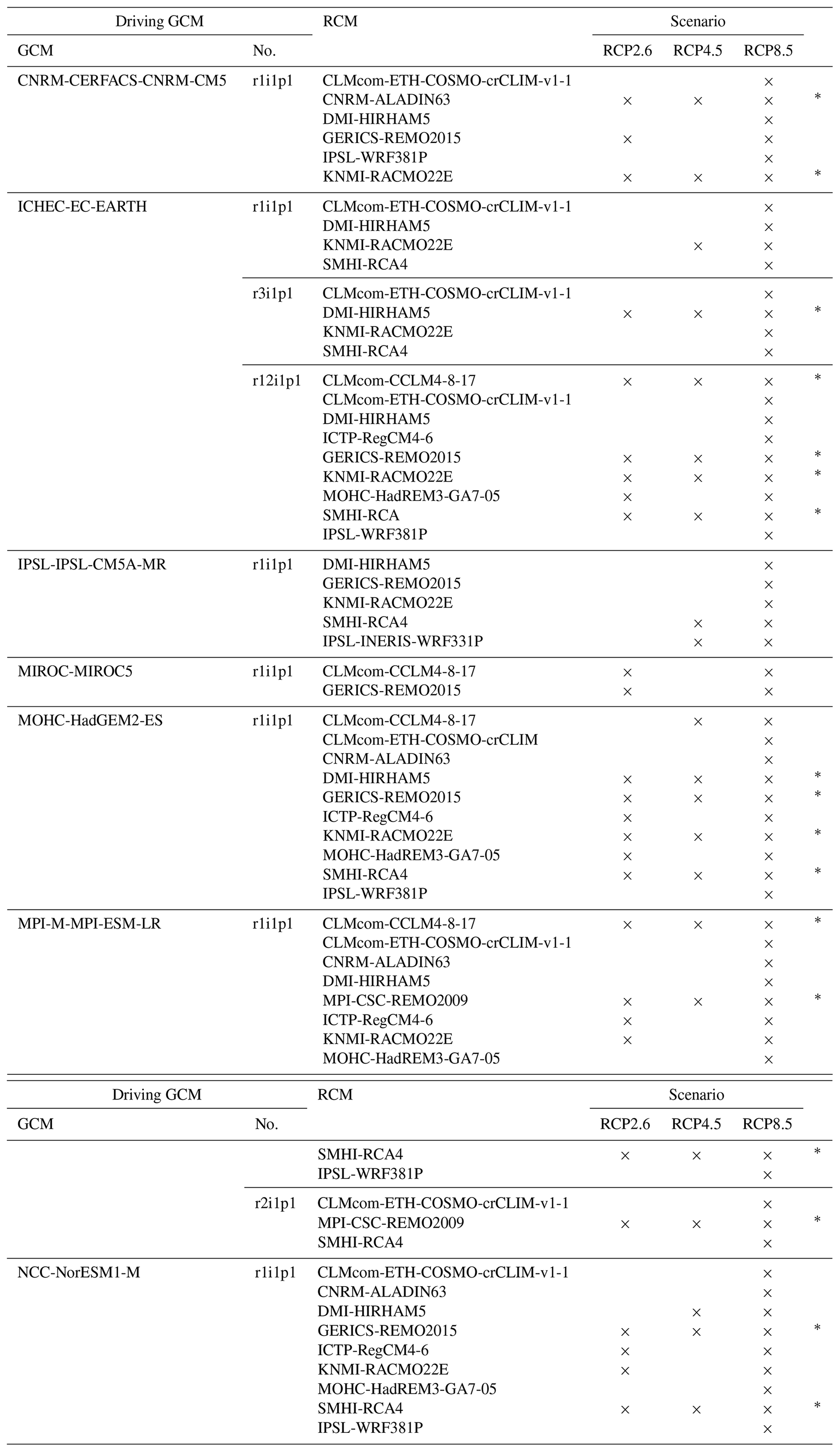
The simulations and their combinations of GCMs, RCMs and RCPs are listed in Table 1. As this study is based on an existing ensemble already in use (SMHI, 2025), we have not excluded any simulations. Adding or removing members would mean that we investigate another ensemble than the one used in the SMHI climate service. The ensemble was created following a “the more the better”-approach, meaning that as many simulations as possible were included.

2.2 Bias adjustment

To minimise systematic errors, the Euro-CORDEX ensemble was bias-adjusted using the “Multi-scale Bias Adjustment” method available in MIdAS (Berg et al., 2022). MIdAS is based on quantile mapping “day-of-year” adjustments (Themeßl et al., 2011; Wilcke et al., 2013), meaning that the distribution used for adjustment varies for each day of the year. MIdAS aims to preserve trends in future projections and performs similarly to methods that explicitly preserve trends (Berg et al., 2022). As reference data, the SMHI gridded climatology data set (SMHIGridClim; Andersson et al., 2021) was used. SMHIGridClim covers Fennoscandia and the Baltic states (region A in Fig. 1), which means that the bias-adjusted ensemble covers a smaller domain centred over Sweden, instead of the entire European domain. The bias adjustment was applied using the period 1980–2000 as a reference. The variables tas, tasmin, tasmax and pr (see Table 2 for explanations) were adjusted in all grid points within the domain. Hereafter, any mention of the CORDEX RCMs refers to this bias-adjusted ensemble covering Fennoscandia and the Baltic states (region A in Fig. 1).

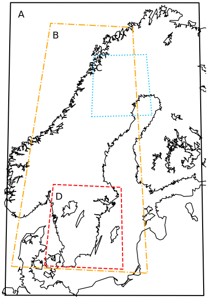
Figure 1 Maps of regions used in analyses in this paper. (A) Fennoscandian region (black, full line) is the domain on which bias adjustment is applied, (B) Scandinavia (dash dotted orange line), (C) northern Sweden (dotted blue line), (D) southern Sweden (dashed red line).

Table 2 Definitions and short names of indicators.

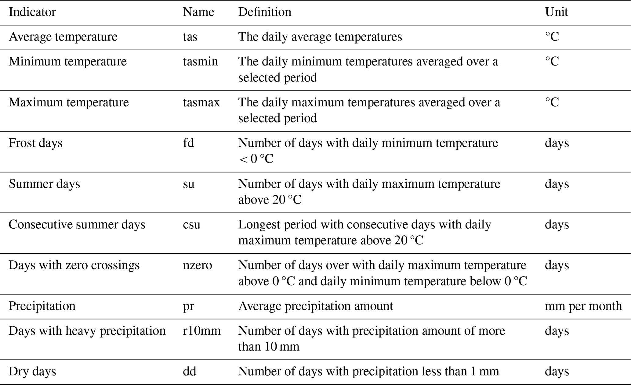
2.3 Calculation of indicators

To assess climate change, a set of climate indicators are calculated using the software package Climix (Bärring et al., 2024). A number of indicators were identified, building on the work of Kjellström et al. (2016), and in collaboration with the Swedish County Administrative Boards and other governmental agencies, to describe relevant changes in climate. The indicators are meant to be relevant for large parts of society, but agriculture (Strandberg et al., 2024a) and the energy sector (Strandberg et al., 2024b) have also been specifically targeted. The indicators used in this study are listed in Table 2. The indicators are presented as averages for the 30-year periods used in the SMHI web service (SMHI, 2025): the reference period 1971–2000 and the future periods 2011–2040, 2041–2070, and 2071–2100. While WMO recommends 1961–1990 as the reference period for describing climate change (WMO, 2017), sseveral RCM simulations begin in 1971, making 1971–2000 a practical compromise.

2.4 Definition of global warming levels

The GWLs are calculated for each driving GCM based on the global mean surface temperature (GMST) using, 1850–1900 as the reference period, following the IPCC-WG1 Atlas protocol (Iturbide et al., 2022). A GWL is reached when the GMST for a moving 20-year time window first exceeds that level. For example: GWL2 occurs when the GMST for the first time is 2 °C higher than during the reference period. The timing of a GWL is represented by a central year. In this study we use 30-year periods for each GWL stretching from 15 years before the central year to 14 years after.

We analysed GWL1.5 and GWL2. GWL1.5 is reached in all scenarios, while GWL2 is reached in RCP4.5 and RCP8.5, but not in RCP2.6. Already at GWL3 most of the RCP4.5 simulations are excluded because they do not reach that level of warming. The limited number of scenarios and the smaller ensemble size makes GWL3 less interesting and less useful for this analysis.

2.5 GCM ensembles

The bias adjusted CORDEX RCMs are compared to two GCM ensembles.

• CORDEX GCMs: This ensemble consists of the GCMs used to drive the RCMs (leftmost column in Table 1). Ensemble sizes are 5, 9 and 9 for scenarios RCP2.6, RCP4.5, and RCP8.5, respectively. It includes several realisations for some GCMs since these are used to force RCMs.

• CMIP5 GCMs: This ensemble includes all CMIP5 models available on the Earth System Grid Federation, but restricted to one realisation per GCM to avoid overweight on certain GCMs. Ensemble sizes are 24, 28 and 34 for scenarios RCP2.6, RCP4.5, and RCP8.5, respectively.

The GCMs are not bias-adjusted. For all GCMs, the grid points within the Fennoscandian region (A in Fig. 1) are used to calculate ensemble mean and spread for the region. For both GCM ensembles, GMST values are calculated as 30-year averages for the reference period 1971–2000 and the future periods 2011–2040, 2041–2070, and 2071–2100.

2.6 Selection and analyses of sub-ensembles

We aim to study the relative importance of the choice of RCP, GCM, and RCM at a specific GWL. To create a consistent ensemble across RCPs, we select only the combinations of GCMs and RCMs that simulated all three scenarios – RCP2.6, RCP4.5, and RCP8.5 (indicated with an asterisk in Table 1). From these 17 combinations of GCMs, RCMs, and RCPs (i.e., 51 RCM simulations), we construct sub-ensembles where all 17 members share the same RCP, GCM, or RCM. We refer to this ensemble as RCM17. Using the full CORDEX RCM ensemble would make it difficult to separate the effects of different ensemble sizes and the effects of models or scenarios. The RCM17 ensemble is used in Sect. 3.5.

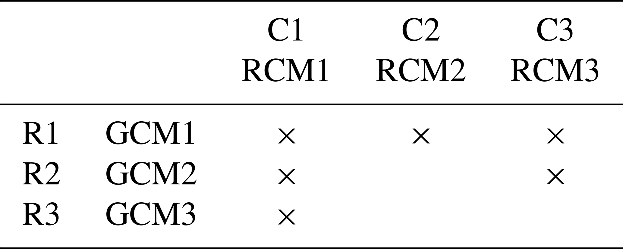
To illustrate the procedure, consider a hypothetical case with three GCMs (GCM1-3) and three RCMs (RCM1-3) combined in different ways (Table 3). A sub-ensemble using only GCM1 would include all RCMs forced by GCM1, i.e., the simulations in row R1 in Table 3 (three simulations). Similarly, the sub-ensemble based on GCM2 consists of two simulations. Sub-ensembles using only one RCM include all simulations with that RCM forced by different GCMs, i.e., one of the columns C1–C3. For example, the sub-ensemble based on RCM1 has three simulations. Sub-ensembles based on a single emission scenario include all simulations run with that scenario.

Table 3 Hypothetical sketch of how three GCMs (GCM1-3) could be downscaled by three RCMs (RCM1-3) and how the sub-ensemble strategy works.

Seven GCMs are combined in various ways with seven different RCMs, resulting in 2 RCP-based, 7 GCM-based, and 7 RCM-based sub-ensembles. To determine whether any model combination differs significantly from the others, we perform two statistical tests under the null hypothesis that any two ensembles have the same average. We use a one-way ANOVA (Analysis of variance) (Press, 1972) test, which tests whether two or more groups share the same average. If the number of groups is equal to 2 – as in the case of RCP-based ensembles – a one-way ANOVA is the same as a student's t-test.

The ANOVA test does not indicate which sub-ensemble is different from the others, if any. Therefore, we apply a post-hoc test: Tukey's honestly significant difference (Tukey, 1949). This test is performed after a successful ANOVA test and compares all sub-ensembles pairwise using a studentised q distribution. The tests are conducted for two regions representing different climatic conditions in Sweden: one in the north and one in the south (regions C and D in Fig. 1). A significance level with a family-wise error of 95 % is used, meaning that the probability of one or more false positives among all points points is 5 % instead of a 5 % false positive rate in each individual grid point if no correction is applied. The analyses were made for tas, csu, tasmin, tasmax, pr, dd, cdd, su, r20mm and nzero.

3 Results and discussion

We begin by describing average climate changes according to the CORDEX RCM ensemble. To better understand these trends, we relate them to the trend in GMST in the driving GCMs (CORDEX GCMs). This is followed by a comparison of ensemble spread between CORDEX RCMs, CORDEX GCMs and a larger ensemble of CMIP5 GCMs to assess how much of the potential spread that is lost by not using all available GCMs. Section 3 is concludes by an investigation of how the description of a GWL based on the RCM17 ensemble is influenced by the GCMs, RCMs and RCPs of which it is constructed.

3.1 Projected change in temperature and temperature-based indicators

The mean temperatures (tas) are projected to increase in all seasons and under all emission scenarios across the domain (Fig. 2). By the end of the century, the annual mean temperature in Sweden is expected to rise by 1–2 °C under RCP2.6, 2–4 °C in RCP4.5, and 4–6 °C under RCP8.5, with larger increases in the north than in the south. The changes scale consistently: RCP8.5 in the near future shows similar warming to RCP2.6 in the mid-century; and RCP8.5 in the mid-century is similar to RCP4.5 at the end of the century (Strandberg et al., 2024a).

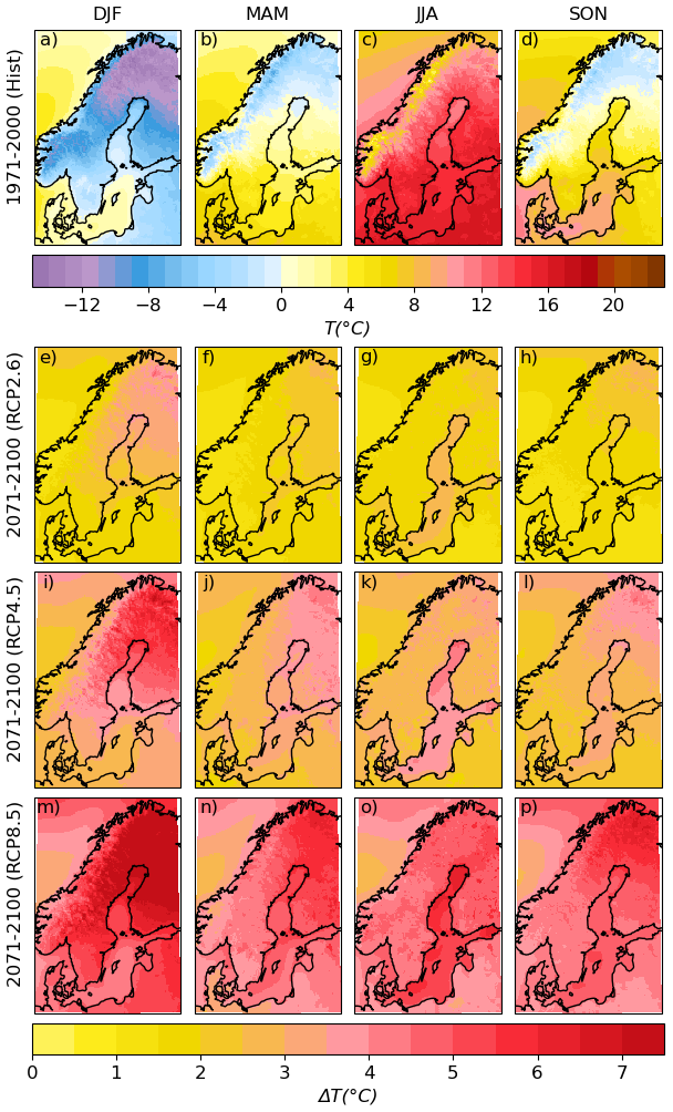
Figure 2 Ensemble mean temperatures of the CORDEX RCMs (°C) in winter (DJF, first column), spring (MAM, second column), summer (JJA, third column) and autumn (SON, fourth column). First row shows absolute values for 1971–2000. Rows 2 to 4 show anomalies from 1971–2000 to 2071–2100 according to scenarios RCP2.6, RCP4.5 and RCP8.5, respectively.

In Fennoscandia, we highlight two climate change patterns for temperature: winter is the season with the fastest warming rate, and the northern parts of the region are warming faster than the southern parts. Under RCP2.6, the warming in winter is 1.5–3.5 °C from south to north (Fig. 2e) and 1.5–2 °C in summer (Fig. 2g). Under RCP8.5, the corresponding numbers are 4.5–8 °C in winter (Fig. 2m), and 4–5 °C in summer (Fig. 2o). This means that warming is larger in winter, but also the difference between north and south.

The temperature change is especially large for the daily minimum temperature (tasmin) (Fig. 3a). For example, under RCP4.5, the increase in tasmin is 3–6.5 °C, compared to an increase in annual tas of 2–4 °C. The increase in daily maximum temperature (tasmax) is comparable to tas, 2–3.5 °C (Fig. 3b). A warmer climate means fewer cold days and more warm days. Accordingly, the number of frost days (fd) is projected to decrease, though relatively uniformly across the domain (Fig. 3c). RCP4.5 gives a reduction of 40–50 d in most of Fennoscandia and the Baltic countries. The change is somewhat smaller in parts of the Scandinavian mountain chain (a decrease in fd with 30–40 d), and larger over the Bothnian Sea and Bothnian Bay (a reduction of 65 d or more). See Fig. S1 in the Supplement for absolute values of the indicators in 1971–2000 and Figs. S2–S4 for climate anomalies in all scenarios RCP2.6, RCP4.5 and RCP8.5.

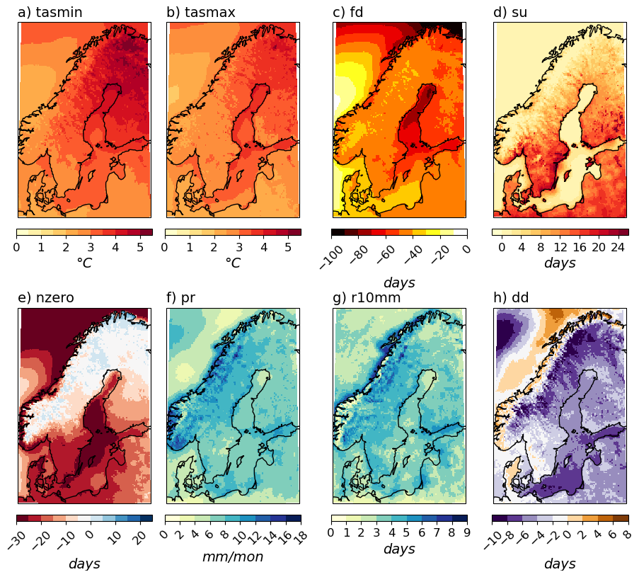
Figure 3 Annual climate change anomalies in the CORDEX RCMs between 1971–2000 and 2071–2100 according to scenario RCP4.5. The maps show ensemble means of (a) daily minimum temperature (tasmin, °C), (b) daily maximum temperature (tasmax, °C), (c) number of frost days (fd, days), (d) number of summer days (su, days), (e) number of days with zero crossings (nzero, days), (f) mean precipitation (pr, mm per month), (g) number of days with heavy precipitation (r10mm, days) and (h) dry days (dd, days). See Table 1 for definitions of the indicators.

Under RCP4.5, the increase in the number of summer days (su) ranges from zero – or just a few days in large parts of the mountain chain and most sea areas – to 20–24 d in southern Sweden and Denmark (Fig. 3d). The number of days with zero crossings (nzero) shows a general decrease on the annual scale (Fig. 3e). In winter, however, nzero increases in most of the domain, except for Denmark, southern Sweden and the Baltic countries (Fig. S5). In these areas, temperatures will not drop below zero degrees as often, whereas in parts of northern Sweden the increase is as much as around 10 d (roughly corresponding to an increase of 50 %).

3.2 Projected change in precipitation and precipitation-based indicators

The annual average precipitation shows a general increase in the future (Fig. 3f). Under, RCP4.5 the increase in annual average daily precipitation is 5–10 mm per month in large parts of the domain, with increases along the Norwegian west coast of up to 15 mm per month. Under RCP2.6, the increase is smaller, 2–6 mm per month (Fig. S2), and in RCP8.5 larger, 8–15 mm per month (Fig. S4). For most of the domain, the increase is larger in winter and smaller in summer compared to the annual change (Figs. S5–S8). Denmark and southern Sweden show summer precipitation changes close to zero. On the annual scale, all models agree on the sign of change in most of the domain and all RCPs (Fig. 3, Figs. S2–S4). The signal is least robust in RCP2.6 because the change is smaller and precipitation generally has large variability. The number of days with heavy precipitation (r10mm) is projected to increase with 3–5 in most of the domain (compared to 10–12 d in the reference period) (Fig. 3g). The change is smaller in RCP2.6 (up to +2 d) and larger in RCP8.5 (+4–8 d) (Figs. S1g & S2g). The number of dry days is projected to decrease by 1–8 d (Fig. 3h). However, the signal is not robust: half of the ensemble members project an increase in dry days, while the other half project a decrease.

3.3 Local trends in climate indicators related to global warming

Climate change is unevenly distributed across the globe. In Scandinavia, like most of Europe, the overall warming since pre-industrial times has been about twice the global mean at the end of the 20th century (Schimanke et al., 2022; WMO, 2023). In this section, we take a look at how specific features of local climate change in the CORDEX RCMs relate to the change in global mean surface temperature (GMST) in the CMIP5 GCMs (Fig. 4).

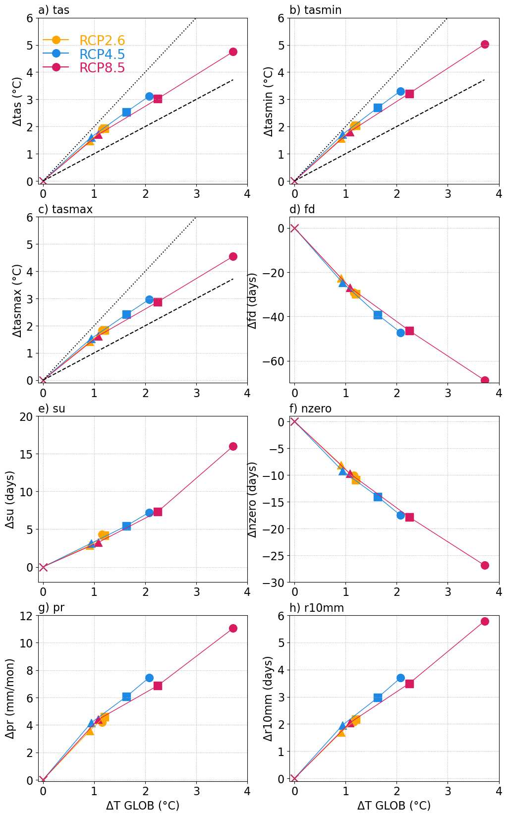
Figure 4 Changes relative to 1971–200 for the Fennoscandian domain (region A in Fig. 1) in the CORDEX RCMs (y-axes) against that in global annual temperature in the driving CORDEX GCMs (x-axes), relative to the period 1971–2000. Different indicators are calculated based on RCM data: (a) mean temperature (tas, °C), (b) minimum temperature (tasmin, °C), (c) maximum temperature (tasmax, °C), (d) no. of frost days (fd, days), (e) no. of summer days (su, days), (f) no. of days with zero crossings (nzero, days), (g) precipitation (pr, mm per month), (h) no. of days with heavy precipitation (r10mm, days). Markers represent the periods 1971–2000 (cross), 2011–2040 (triangle), 2041–2070 (square), 2071–2100 (circle) for emissions scenarios RCP2.6 (green), RCP4.5 (orange) and RCP8.5 (light blue). In panels a-c the one-to-one relationship is shown with a dashed line, and the two-to-one with a dotted line.

The almost two-to-one relationship between global and local temperature is seen for mean, minimum and maximum temperatures until the period 2011–2040 (Fig. 4a–c). Within this period, the ratio between regional and global warming is 1.6–1.8. With increasing global warming, this relationship weakens and approaches a one-to-one relationship between change in global and local temperatures (i.e. parallel to the dotted lines in Fig. 4a–c). In RCP4.5 and RCP8.5 the trend from 2041–2070 to 2071–2100 is roughly one to one (1.1–1.2), suggesting that the faster warming in Scandinavia will slow down as GMST increases. A conclusion of this could be that the ratio between warming in Scandinavia and global warming is at its maximum in the beginning of the 21st century.

For indicators representing cold conditions, the trend gets flatter in RCP8.5, reflecting that the potential for change decreases. For example: the number of frost days cannot be less than zero. For warm indicators, the trend instead steepens. The number of summer days is based on a temperature threshold, which means that there is a sudden effect when temperatures exceed the threshold. Consequently, the increase may be limited if the number of days above the threshold is already large.

Indicators for precipitation show continued increase under global warming. Here, results both for pr and r10mm show a slightly weaker trend in RCP8.5 than in the other two scenarios.

3.4 Model spread in the CORDEX RCM and CORDEX GCM ensembles compared to the spread in the CMIP5 GCM ensemble

Even though the CORDEX RCM ensemble consists of several simulations using different GCM-RCM combinations, it may not represent the full potential spread of the climate change signal. To investigate how well the CORDEX RCMs capture the variability within the greater CMIP5 GCM ensemble, the average changes in temperature and precipitation over the Fennoscandian domain (region A in Fig. 1) were calculated. Figure 5 shows that the ensemble spread in the CMIP5 ensembles is larger than in the CORDEX RCM ensemble. In particular, the difference between the minimum and maximum is larger in the CMIP5 GCMs than in the CORDEX RCMs. This could not entirely be explained by differences in ensemble sizes. For example, see the numbers for RCP8.5 in Fig. 5c, where the CMIP5 GCMs and the CORDEX RCMs show large differences in spread although the ensembles are of comparable sizes. In the case of RCP8.5, the 62 members in the CORDEX RCM ensemble use only 7 unique GCMs and 11 RCMs, which is much less than the 34 unique GCMs in the full CMIP5 ensemble. When considering an ensemble consisting only of the 9 GCMs (including different realisations) used to force the RCMs, the spread is much smaller.

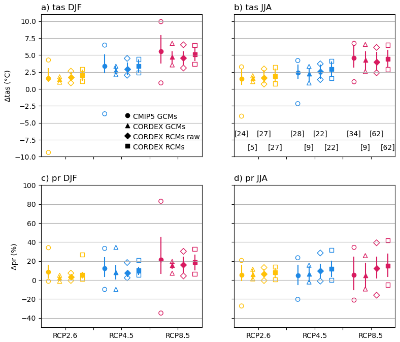
Figure 5 Temperature (tas, °C) (a, b) and precipitation (pr, %) (c, d) anomalies in Fennoscandia 1971–2000 to 2071–2100 for winter (a, c) and summer (b, d) according to the scenarios RCP2.6 (yellow), RCP4.5 (blue) and RCP8.5 (red). The CMIP5 GCMs are represented by circles, the CORDEX GCMs by triangles, the unadjusted raw CORDEX RCMs by diamonds and the CORDEX RCMs by squares. The central marker represents the ensemble mean, the line spans between the 10th and 90th percentiles, open markers show ensemble minima and maxima. Panel (b) also shows the number of members in the respective ensembles.

The CORDEX RCM ensemble is compared to its raw equivalent, where no bias adjustment has been performed, to assess the impact of bias adjustment on the climate change signal. The means and spreads are similar in both RCM ensembles, but the raw ensemble systematically shows smaller changes. Although small, these differences are significant in DJF, and in JJA under RCP8.5.

The ensemble means, however, are quite similar. In general, all ensembles agree on the large-scale differences, and the choice of emission scenario is of greater importance than the construction of the ensemble (Fig. 5). The result is the same even when examining smaller regions within the domain (e.g. regions B, C and D in Fig. 1). In conclusion, the Euro-CORDEX ensemble well captures the mean climate change signal, but that the spread is limited compared to the CMIP5 ensemble.

3.5 How the simulated GWL climate is influenced by the choice of GCMs, RCMs and RCPs

Here, we investigate how the characteristics of a certain GWL are influenced by the models and scenarios it is made of. Are all GWL2 the same, even if different models and scenarios are used to calculate them? First, we look at sub-ensembles based on GCMs (all members in a sub-ensemble are forced with the same GCM). Then we examine sub-ensembles based on RCM and RCP (all members of a sub-ensemble use the same RCM and RCP, respectively). Statistically significant differences are assessed using an ANOVA analysis (see Sect. 2.5).

3.5.1 Sub-ensembles based on driving GCMs

The results for sub-ensembles forced by the same GCM (all members of a sub-ensemble are forced with the same GCM, see Methods) are exemplified by temperature (tas) and annual number of summer days (su, see Table 2 for definitions). Figure 6 shows which sub-ensembles are significantly different from each other in the case of tas. All sub-ensembles from 1 to 7 are compared pairwise to see if they are significantly different. As an example, a green box at row 5 and column 1 means that sub-ensembles 5 and 1 are significantly different. In winter, the average temperature change at GWL2 is +1.5–2.8 °C in the south and +1.7–4.2 °C in the north, depending on the chosen sub-ensemble (Fig. S9). Despite the rather large spread in warming the significant differences between sub-ensembles are not systematic in winter. However, in summer, where the temperature change is +1.0–2.5 °C in the south and 1.3–2.9 °C in the north (Fig. S9), there are systematic significant differences between sub-ensembles. The two sub-ensembles with the largest warming, labelled 4 & 7, are significantly different from the other sub-ensembles (green boxes at lines 4 and 7, and columns 4 and 7 in Fig. 5). This pattern is also, to some extent, seen for su (Fig. 7). In the south, sub-ensemble 7 is significantly different from 5 of the other sub-ensembles; in the north sub-ensemble 4 is significantly different from 5 other. For precipitation, the difference at GWL2 is small compared to the variability within each sub-ensemble. Only a few pairs of sub-ensembles are significantly different (none in summer in the north), but not in a systematic way (Fig. S10).

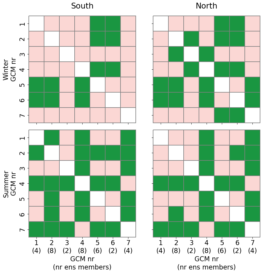
Figure 6 Matrix of significant differences in temperature (tas) between GCM-based sub-ensembles within RCM17, for southern Sweden (South, region C in Fig. 1) and northern Sweden (North, region D in Fig. 1). Green colours indicate significant differences between two sub-ensembles and pink non-significant differences. White colours indicate that an ensemble is compared with itself. Numbers indicate sub-ensemble numbers, with the number of members in parenthesis.

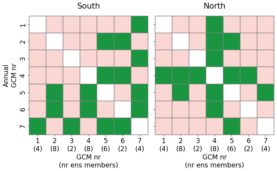
Figure 7 Same as Fig. 6 but for annual number of summer days (su, see Table 2 for definitions).

The choice of GCM can have a large impact on the ensemble. The difference in simulated change in tas can be up to 2 °C depending on the driving GCM; this does however, transfer into consistent significant differences for only two sub-ensembles.

3.5.2 Sub-ensembles based on RCMs

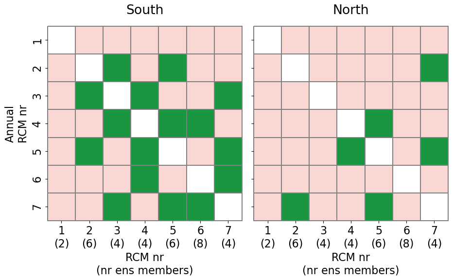
Next, we examine sub-ensembles where the same RCM is used (all members of a sub-ensemble use the same RCM). Figure 8 shows which sub-ensembles are significantly different from each other with regards to tas. The difference in projected change is about 1 °C between the sub-ensemble with the smallest and the largest change. Still, sub-ensemble no. 7 is the only sub-ensemble with systematically significant differences; in winter in the northern region and in summer it's different to all, or all but one, of the other ensembles. Sub-ensemble no. 7 is the sub-ensemble with the smallest temperature increase. For su, there are more significant differences in the southern region than in the northern, reflecting the larger variability in su in the south (Fig. 9). There are however only two sub-ensembles that are significantly different from the other sub-ensembles. Again, sub-ensembles 4 and 7, with a low number of su. For precipitation, the difference at GWL2 is small compared to the variability within each sub-ensemble. Only a few pairs of sub-ensembles are significantly different (in winter in the north one), but not in a systematic way (Fig. S11).

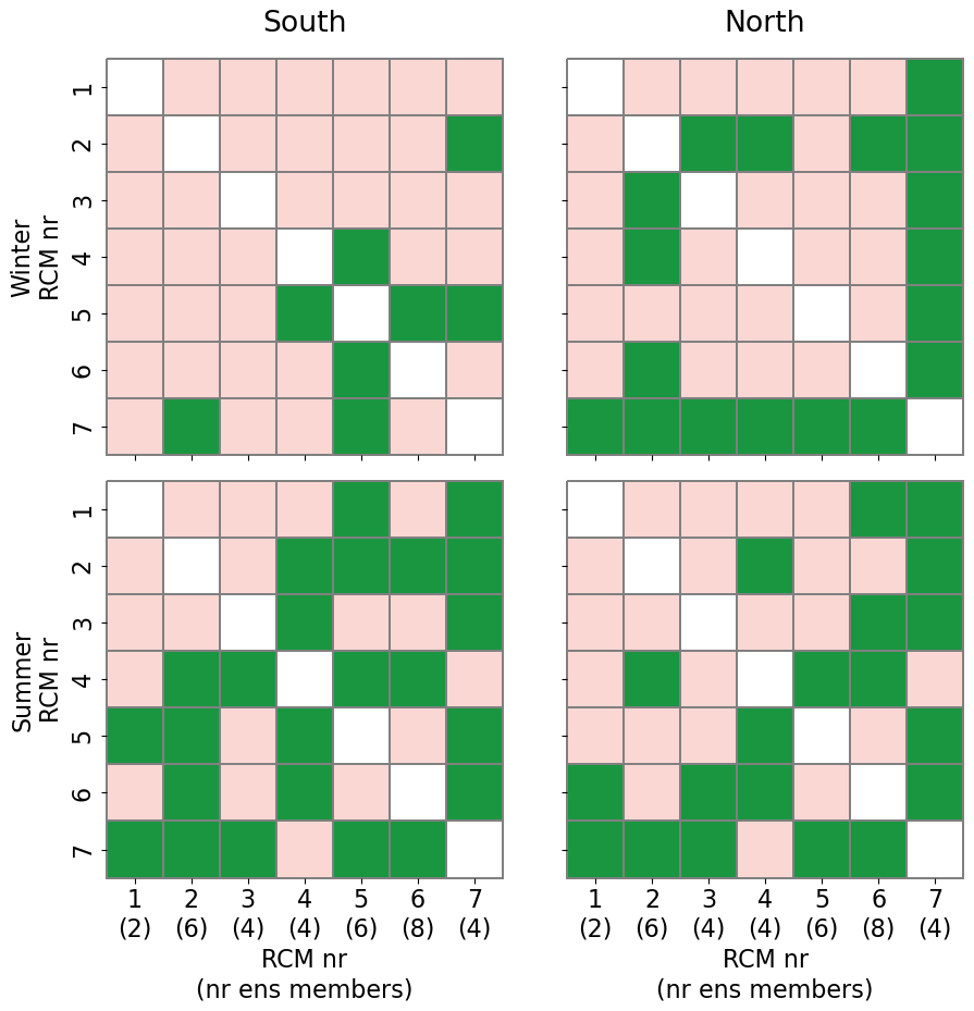
Figure 8 Matrix of significant differences in temperature (tas) between RCM-based sub-ensembles within RCM17, for southern Sweden (South, region C in Fig. 1) and northern Sweden (North, region D in Fig. 1.). Green colours indicate significant differences. Numbers indicate sub-ensemble numbers, with the number of members in parenthesis.

Figure 9 Same as Fig. 8, but for annual su.

3.5.3 Sub-ensembles based on RCPs

As a last step, we examine sub-ensembles using the same RCPs. This analysis addresses whether the choice of RCP affects the description of a GWL climate. Here, only two sub-ensembles are compared. Differences between the ensembles based on RCP4.5 and RCP8.5 are generally small and not statistically significant (see Fig. S12 for tas). RCP8.5 gives larger anomalies in tas, tasmin and tasmax in summer in all regions. The difference compared to RCP4.5 is around 0.15 °C and just below the 95 % confidence threshold. The difference in all other indicators are insignificant on the 99 % level.

Inevitably, the characteristics of a climate model ensemble are determined by the simulations it comprises. Using other models will not yield identical results. These differences are however not systematic in any way, and mostly not significant. Even though an ensemble should be constructed with care, the role of the composition should not be exaggerated.

4 Discussion

4.1 The role of the models used on projected climate change

The projections of future climate presented here are consistent with other studies of the European climate (e.g. Coppola et al., 2021; Ranasinghe et al., 2021) and the climate in the Nordic region (e.g. Christensen et al., 2022). The ensemble used here is an unbalanced `ensemble of opportunity', as no pre-selection of models was applied. In such cases there is a risk that some models are under- or over-represented, which influences the ensemble mean (Evin et al., 2021; Sobolowski et al., 2025). On the other hand, information is lost when simulations are discarded, and natural variability is best sampled by single-model large ensembles (e.g. von Trentini et al., 2019; Maher et al., 2020). Furthermore, we note that different selections of individual GCM-RCM-RCP-combinations can have significant impact on the resulting ensemble as illustrated above. In the end, it is difficult to say that there is one approach that is always the most suitable. Different choices in the construction of an ensemble can be made and justified depending on the aim.

Insufficient aerosol forcing is proposed as a reason for the observed underestimation of the trend in summer temperature in RCMs over central Europe compared to observations (e.g. Boé et al., 2020; Schumacher et al., 2024). However, the difference in summer warming between CORDEX and ERA5 is small in southern Sweden and Finland, and actually positive in Norway and northern Sweden (Schumacher et al., 2024). Bias adjustment may alter the climate change signal, but this is generally seen as an improvement of the signal (Gobiet et al., 2015). MIdAS, the bias adjustment method used here, is shown to add a small increase in the climate change signal for both temperature and precipitation in Europe (Berg et al., 2022). The effect of bias adjustment on indicators remains uncertain and should be studied in the future.

A notable feature of the scaling between local and global climate change is seen for the precipitation indicators (Fig. 4g, h). Here, there are clear differences between RCP4.5 and RCP8.5 even at the same level of global warming. It has previously been shown on the global scale that the response in precipitation depends on both surface warming and radiative effect of increased amounts of greenhouse gases (Pendergrass et al., 2015). The net effect of these depends on the RCP scenario. Furthermore, the aerosol forcing is different in the different scenarios. This would make GWLs less suitable for precipitation. On the European scale this is further complicated by local features. The weaker response in precipitation could be a consequence of drier conditions over the European continent leading to excessive evaporation and soil drying (e.g. Tuel and Eltahir, 2021).

4.2 Difference in model spread between GCM and RCM ensembles

In this study we show that the spread between the driving GCMs was larger than the spread between RCMs, even when the RCM ensemble contained more members. This is supported by Kjellström et al. (2018). A potential explanation is that number of members is not the same as number of models. Previous studies show that multi-model ensembles have larger spread than single-model ensembles of similar or even larger sizes (von Trentini et al., 2019; Maher et al., 2021), which is perhaps not surprising given that different models have different physics. Consequently, a multi-model ensemble can provide a wider response to forcing and natural variability than a single-model ensemble. This is supported by the observation that the ensemble mean in the CORDEX GCM ensemble is not affected in any major way when additional realisations from the same GCM are included. Adding more realisations likely improves estimates of natural variability and extremes, but does not influence the mean values as much, as all realisations simulate the same climate (as opposed to simulations with different physics or forcing).

In this study, bias-adjusted RCMs are compared to non-adjusted GCMs. Bias adjustment may reduce model spread in absolute values since systematic biases are minimised and all models are forced towards the reference data. Here, it systematically increases the climate change signal in the RCM ensemble. Although this increase is in many cases significant, it is relatively small, and the raw RCM ensemble is more similar to the bias-adjusted RCM ensemble than to any of the GCM ensembles. Consequently, the differences between GCMs and RCMs are likely not explained by the application of bias adjustment.

Another explanation for differences in model spread are inconsistencies in forcing between the RCMs and the driving GCMs, where aerosol forcing probably is the most prominent factor in the context of this study (Taranu et al., 2023). This problem is indeed seen in both GCMs and RCMs, but only for summer in central Europe (Schumacher et al., 2024).

4.3 On the characteristics of GWL ensembles

Since GWLs are in fact used for many different purposes it is necessary to investigate the characteristics of GWL ensembles – especially how RCPs influence the GWL climate. Our study shows, for a broad range of indicators, that the choice of RCPs has minimal effect on the GWL climate. Furthermore, it is difficult to demonstrate that including specific GCMs or RCMs influence the GWL climate in a significant way. This is perhaps expected considering that GCMs and RCMs are not independent (Sørland et al., 2018) and that the uncertainty in climate change due to GCMs can be as large as the uncertainty due to RCMs (Evin et al., 2021).

A caveat to our findings relates to the small number of members in the sub-ensembles. Sub-ensemble sizes of 2–8 make it difficult to draw robust conclusions. Small samples reduce the power of the ANOVA test to detect differences between sub-ensembles and are more likely to fail to reject a false null hypothesis. In any case, this – and similar – ensemble is what is used to create GWL ensembles, and they must therefore be evaluated as much as possible. Adding more members would increase the statistical power, but would also alter the ensemble's composition. We just have to do what we can with the ensemble at hand. A more solid evaluation could perhaps be achieved if AI or emulators were first used to fill all gaps in the matrix. That would enable a balanced comparison across GCMs and RCMs.

We performed our analysis on GWL1.5 and GWL2, and our conclusions only apply to these specific GWLs. It would be interesting to expand the analysis to more GWLs, but there are practical limitations to this. Smaller GWL increments would mean larger overlap between GWLs, making it difficult to draw robust conclusions about the differences between GWLs. Furthermore, most RCP4.5 simulations do not reach GWL3 which means that the ensemble size would be heavily reduced, making the statistical analysis less solid. Also, if only one RCP reaches GWL3, it is not possible to investigate the role of RCPs in the construction of a GWL – arguably the most relevant aspect to understand. Studying a broader range of GWLs in an RCM ensemble would require a separate study, a study that would require other simulations, and maybe simulations that do not exist (for example more scenarios that reach GWL3).

5 Summary and conclusions

Global warming in Fennoscandia means higher temperatures, more warm days, and fewer cold days. In southern Sweden the number of summer days is doubled until the end of the century according to RCP4.5. At the same time, the number of frost days decreases by 20 %–50 %. Precipitation increases generally; this shows in increasing mean precipitation, increasing number of days with heavy precipitation and decreasing number of dry days.

The RCM ensemble used here captures, on average, the change pattern from the CMIP5 GCM ensemble. However, the ensemble spread is larger in the CMIP5 ensemble.

The choice of RCP has minimal influence on the GWL2 ensembles. This implies that it would be safe to mix RCPs in the construction of GWL ensembles in order to increase ensemble size, and that a GWL could be based on only one RCP. It should be noted, however, that we only look at mean changes. Trends within a GWL period do indeed depend on the RCP, and this could influence extremes. For example: the last years within a GWL period based on RCP8.5 may be warmer than the last years within a GWL period based on RCP2.6. The largest difference between GWL2 sub-ensembles, regardless of how they are constructed in terms of combining GCMs and RCMs, is seen for temperature-based indices. However, it remains difficult to say whether the choice of GCM or RCM contributes most to these variations.

All studied climate indicators scale approximately linearly to the change in GMST. For indicators based on temperature thresholds, trend slopes may shift when temperatures exceed certain levels. Currently the regional temperature change in Sweden is almost twice as large as the global trend. This ratio will decrease as GMST increases, to more and more approach a one-to-one relationship. This suggests that there is a limit to the feedback mechanisms that now accelerates the warming in Sweden and indicates that the ratio between local and global warming currently may be at its maximum. Furthermore, this means that the steady relationship between global and regional warming that is sometimes assumed in weather attribution and regional warming levels may not remain valid in the future.