Boreal autumn to winter North Atlantic atmosphere–ocean coupling in large ensemble climate simulations

Recent studies have suggested an observed causal relationship between autumn North Atlantic sea surface temperature (SST) anomalies and the phase of the winter North Atlantic Oscillation (NAO). This autumn SST-winter NAO link, which is mediated by turbulent heat fluxes (THF) and baroclinicity, appears to be underestimated in seasonal prediction models, suggesting possible model limitations in representing air-sea coupling. However, strong atmospheric driving of North Atlantic THF and SST variability at seasonal timescales presents a challenge in establishing a causal ocean feedback onto the large-scale atmosphere. This study examines the representation of autumn–winter North Atlantic atmosphere-ocean variability in ERA5 reanalysis data and historical large ensembles from the sixth phase of the Coupled Model Intercomparison Project (CMIP6). Models adequately capture concurrent North Atlantic atmosphere-SST variability within the autumn and winter seasons, when THF and SST tendencies are mainly atmosphere-driven. However, the leading mode of covariance between autumn SST–winter mean sea level pressure (MSLP) in models differs from ERA5. In ERA5, warm SST anomalies in the central North Atlantic in autumn precede a positive winter NAO anomaly. Conversely, the CMIP6 models show, on average, weak cool autumn SST anomalies precede a positive winter NAO with large model spread. Using an atmospheric analogue method, we separate atmosphere- and ocean-driven components of autumn THF variability and assess their respective relationships with winter MSLP variability. In ERA5, the winter MSLP signal associated with ocean-driven autumn THF anomalies is near zero; in contrast, the winter NAO is linked to atmosphere-driven autumn THF variability. This suggests that atmospheric processes, such as tropical-extratropical teleconnections, could explain the autumn THF–winter MSLP relationship in ERA5 described in a previous study, or that SST anomalies arising from autumn atmospheric forcing persist into winter and contribute to a lagged feedback on the atmosphere. CMIP6 models generally underestimate the winter NAO signal associated with atmosphere-driven autumn THF anomalies, which could reflect biases in feedbacks or atmospheric teleconnections.

1 Introduction

The North Atlantic Oscillation (NAO; Hurrell et al., 2003) and the East Atlantic pattern (EAP; Barnston and Livezey, 1987; Hernadez and Comas-Bru, 2025) are the two leading modes of variability in the winter North Atlantic atmospheric circulation on monthly to decadal timescales. Variability in the NAO and EAP indices are associated with changes in the strength and location of the North Atlantic jet stream (e.g., Mellado-Cano et al., 2019; Perez et al., 2024), which affects temperature and precipitation patterns in Europe and North America (Hurrell et al., 2003; Hernadez and Comas-Bru, 2025).

Seasonal prediction systems demonstrate skill in forecasting the winter NAO (e.g., Scaife et al., 2014; Smith et al., 2016; Athanasiadis et al., 2017) and the autumn/early winter EAP (Thornton et al., 2023). However, a body of literature highlights that signal-to-noise ratios of these modes in model predictions are weaker than expected for their level of skill (Eade et al., 2014; Scaife et al., 2014; Smith et al., 2019; Thornton et al., 2023). This underestimation of the predictable signal suggests that key drivers of large-scale North Atlantic atmospheric variability may not be well represented in current models, motivating improved understanding of the drivers and mechanisms of predictability.

Multiple drivers of North Atlantic winter atmospheric variability have been identified including: tropically-forced Rossby wave trains, e.g. from the El Niño Southern Oscillation (ENSO) (Scaife et al., 2017; Jiménez-Esteve and Domeisen, 2018; Thornton et al., 2023); Arctic sea ice anomalies, particularly in the Barents-Kara seas (Koenigk et al., 2016; Wang et al., 2017; Petoukhov and Semenov, 2010; Mori et al., 2014); and stratosphere-troposphere coupling (Scaife et al., 2016; Williams et al., 2025).

Air-sea interactions associated with sea surface temperature (SST) anomalies provide another potential driver of seasonal North Atlantic atmospheric variability (e.g., Ossó et al., 2018; Ferreira and Frankignoul, 2005; Deser et al., 2007; Czaja and Frankignoul, 2002; Kolstad and O'Reilly, 2024). The NAO drives SST variability through fast atmospheric forcing via surface turbulent heat fluxes (THF) and slower timescale oceanic Ekman transport changes, resulting in a tripolar pattern of SST anomalies that emerges as a response to NAO anomalies at seasonal timescales (Cayan, 1992; Deser and Timlin, 1997; Marshall et al., 2001; Eden and Willebrand, 2001). The EAP also drives SST anomalies at seasonal timescales, with a positive EAP associated with a dipolar SST pattern, characterised by warming in the central-subpolar North Atlantic and cooling in the Nordic Seas (Gastineau and Frankignoul, 2015). Although less extensively studied compared to the NAO SST tripole, this response is thought to arise primarily through surface turbulent heat flux anomalies, which drive ocean heat loss and imprint the atmospheric circulation pattern on SSTs (Cayan, 1992; Deser et al., 2010).

While the North Atlantic SST response to atmospheric forcing has long been acknowledged, there has also been interest in North Atlantic SST anomalies contributing to atmospheric predictability through an ocean-driven feedback. Ferreira and Frankignoul (2005) showed that the tripolar SST anomalies caused by the NAO can induce lower tropospheric diabatic heating through anomalous THF, enhancing transient eddy activity and reinforcing NAO-like pressure patterns. Similarly, Deser et al. (2007) explored atmospheric adjustment to prescribed SST anomalies, showing that while the initial atmospheric adjustment occurs on timescales of days to weeks, the full circulation response emerges over several months, suggesting that antecedent SST anomalies may contribute to seasonal atmospheric predictability. Consistent with these results, statistical analyses have identified links between autumn and early winter SST anomalies and the subsequent winter NAO (Czaja and Frankignoul, 2002; Wang et al., 2017; Kolstad and O'Reilly, 2024). Kolstad and O'Reilly (2024) highlighted the role of latent heat release and lower-tropospheric baroclinicity as key mediators of the relationship between November SST anomalies and the winter NAO. However, these mediators were found to be weaker in a seasonal prediction model than in a reanalysis dataset (Kolstad, 2026). Studies of coupled atmosphere-ocean climate models and decadal forecast models have also shown that the covariance between decadal North Atlantic SST anomalies and the NAO appears weaker than observed (Bonnet et al., 2024; Patrizio et al., 2025), suggesting that climate models may struggle to accurately represent the mediating processes.

A key challenge in diagnosing the influence of North Atlantic SST anomalies on the atmosphere is the strong bi-directional air-sea coupling and the autocorrelative behaviour of the North Atlantic ocean and atmosphere (Coëtlogon and Frankignoul, 2003; Keeley et al., 2009), which can confound the isolation of causal relationships. To overcome this challenge, Patterson et al. (2024) proposed an atmospheric circulation analogue methodology, which exploits the fact that a local ocean influence on the atmosphere must primarily be communicated through anomalous surface THF independent of the atmospheric state. By combining information from years with similar atmospheric circulation patterns but different SST anomalies, they estimated the component of the anomalous THF driven by the atmospheric state. This approach allows the THF anomaly attributable to atmospheric variability to be isolated, with the residual interpreted as the ocean-driven component.

Another related challenge in isolating the influence of local North Atlantic SST anomalies on the atmosphere is the potential for confounding influences from the various aforementioned remote drivers. To overcome the challenge of evaluating modelled atmosphere-ocean coupling in the presence of internal variability, large initial condition ensembles allow a fairer evaluation of model performance by accounting for the fact that observation-based estimates may be influenced by internal variability. This study investigates the representation of North Atlantic coupled atmosphere–ocean variability in boreal autumn and winter using historical large ensemble simulations from multiple climate models, with an emphasis on the level of agreement between reanalysis-based estimates and modelled coupling.

The remainder of the paper is laid out as follows. Section 2 describes the data, methods and overall analysis strategy, Sect. 3 presents results, where we first assess the representation of contemporaneous atmosphere-ocean co-variability within the autumn and winter seasons. We then explore the dominant lagged relationships between autumn and winter and how these are captured in the models. Finally, we determine the relationships between the autumn atmospheric and oceanic driven THF anomalies and the winter atmosphere, assessing whether the ocean-driven component may act as a precursor to the winter NAO. Section 4 discusses the implications of the results and summarises the conclusions.

2 Datasets and methods

2.1 Model data

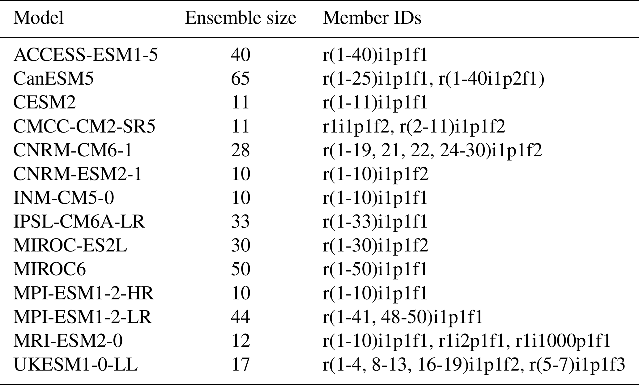
The analysis uses historical simulations from 14 coupled atmosphere-ocean climate models participating in the sixth phase of the Coupled Model Intercomparison Project (CMIP6) (Eyring et al., 2016). The models are chosen based on the number of ensemble members for which the required data were available on the Earth System Grid Federation, with a minimum ensemble size of 10. Monthly mean SST (“tos”), MSLP (“psl”) and THF (sum of “hfls” and “hfss”) were used to characterise atmosphere-ocean variability. The models and the corresponding ensemble members analysed are shown in Table 1.

Table 1 CMIP6 models used in the study, number of ensemble members and corresponding member IDs.

2.2 Reanalysis data

The European Centre for Medium Range Weather Forecasts (ECMWF) Reanalysis v5 (ERA5) (Hersbach et al., 2020) was used to evaluate the modelled relationships in the North Atlantic domain (90° W–40° E, 20–85° N). The analysis focuses on the common period between the datasets of 1940–2014. All data were regridded to a 1° × 1° horizontal grid for consistency. Seasonal-mean anomalies are used throughout, with no detrending applied. The low-frequency variability is removed by subtracting an 8-year running mean from the anomaly fields in order to focus on interannual variability.

2.3 Methods

2.3.1 Overview of analysis strategy

This study evaluates whether CMIP6 models reproduce the observed relationship between autumn North Atlantic SSTs and winter atmospheric circulation, and whether that relationship has an ocean driver. The analysis uses three steps to separate the simultaneous atmospheric forcing of SSTs and the ocean driven component. First, contemporaneous Maximum Covariance Analysis (MCA) of SST and MSLP within autumn and winter assesses atmospheric forcing of SST, which dominates on seasonal timescales. Comparison with univariate EOFs tests whether the coupled modes reflect the dominant variability of each field. Second, lagged MCA of autumn SST and winter MSLP tests whether models reproduce the observed autumn SST-winter MSLP relationship. Lagged covariance alone does not demonstrate a feedback, therefore third, we use circulation analogues to separate autumn THF into atmosphere-driven and ocean-driven components, and test which one is linked to the winter NAO.

2.3.2 Maximum covariance analysis

MCA is used to identify the dominant modes of spatio-temporal covariance between North Atlantic mean sea level pressure (MSLP) and SST, applied separately within autumn (September–November) and winter (December–February) seasons, and across seasons. The approach is the same as that followed by Czaja and Frankignoul (2002).

Let S be the SST anomaly matrix and P the MSLP anomaly matrix (each with p spatial grid points × n temporal samples). The cross-covariance matrix between the two fields is:

$$\begin{array}{}\text{(1)}& {\mathbf{C}}_{\mathrm{SP}}={\displaystyle \frac{\mathrm{1}}{n}}{\mathbf{PS}}^{\mathrm{T}}.\end{array}$$

Singular value decomposition (SVD) of the cross-covariance matrix yields:

$$\begin{array}{}\text{(2)}& {\mathbf{C}}_{\mathrm{SP}}={\mathbf{UDV}}^{\mathrm{T}},\end{array}$$

where U and V are matrices containing the left and right singular vectors, representing spatial patterns in the SST and MSLP fields, respectively. D is a diagonal matrix with singular values d_k ordered in decreasing magnitude. Each pair of singular vectors defines a coupled mode that maximises the covariance between the two fields and explains a portion of the total cross-covariance.

The associated expansion coefficients are obtained by projecting the anomaly fields onto their respective singular vectors. Homogeneous patterns are defined as the correlation between each field and its own expansion coefficients, while heterogeneous patterns are obtained by correlating each field with the expansion coefficients of the other field. These patterns highlight the spatial structures associated with coupled SST–MSLP variability.

The relative importance of each mode is quantified using the squared covariance fraction (SCF):

$$\begin{array}{}\text{(3)}& {\text{SCF}}_k={\displaystyle \frac{d_k^{\mathrm{2}}}{{\sum }_{i=\mathrm{1}}^K{d}_i^{\mathrm{2}}}},\end{array}$$

which represents the proportion of total squared covariance explained by mode k.

2.3.3 Circulation analogue decomposition

We use the circulation analogue method of Patterson et al. (2024) to explore the relative roles of atmospheric and oceanic forcing of autumn THF anomalies. The method estimates the atmospheric circulation-driven component of THF anomalies using an atmospheric analogue technique that samples other years in the dataset with a similar MSLP field.

For each year in the dataset, i, the seasonal mean MSLP anomalies within the Euro-Atlantic domain (90° W–40° E, 20–85° N) are compared with all other years in the dataset using the area-weighted Euclidean distance. A subset of N_a years with the smallest Euclidean distances from year i are identified as candidate analogue years. From this subset, N_s years are randomly selected and used to reconstruct the MSLP anomaly field for the target year as a weighted linear sum:

$$\begin{array}{}\text{(4)}& {\text{MSLP}}_{i,j}=\sum _k{a}_k{\text{MSLP}}_{k,j},\end{array}$$

where a_k is the weight assigned to the kth analogue year, determined based on its proximity to the target year's anomalies.

The analogue years and their weights, a_k, are then used to estimate the THF anomaly at each gridpoint, j, associated with the circulation state in the target year (THF${}_{\mathrm{circ},i,j}$) independent of the SST state:

$$\begin{array}{}\text{(5)}& {\text{THF}}_{\mathrm{circ},i,j}=\sum _k{a}_k{\text{THF}}_{k,j}.\end{array}$$

This assumption relies on the distribution of weights, a_k, being sufficiently broad such that THF_circ is not derived from only a small number of strongly weighted years which may not ensure independence of the SST state. The procedure is repeated N_r times using different random subsets of analogue years, and the resulting reconstructions are averaged to obtain the estimate of THF_circ,i. In this study, N_a, N_s and N_r are 50, 30 and 100, respectively. Patterson et al. (2024) demonstrated using a 500-year control simulation that the result is not strongly sensitive to the choice of these parameters and we have verified this for the shorter ERA5 dataset (not shown).

The residual between THF_i and THF_circ,i is inferred to be the THF component in year i primarily associated with the oceanic state (THF_res,i):

$$\begin{array}{}\text{(6)}& {\text{THF}}_i={\text{THF}}_{\mathrm{circ},i}+{\text{THF}}_{\mathrm{res},i}.\end{array}$$

THF_res,i encompasses concurrent ocean-driven variability, as well as the memory and persistence of preceding SSTs.

The characteristics of spatio-temporal variability in autumn THF, THF_circ and THF_res are assessed by computing the first two Empirical Orthogonal Functions (EOFs) and corresponding PC timeseries. The respective association of autumn THF with the winter NAO is assessed by linearly regressing the winter MSLP onto PC1 and PC2 of the THF component timeseries.

2.3.4 NAO and EAP indices

The NAO and EAP indices are defined as the first and second EOFs of seasonal mean MSLP anomalies. Indices are computed per ensemble member, then used separately. We multiply the EOF patterns by the standard deviation of their principal component (PC) timeseries to recover the patterns in units of hPa. EOF1 exhibits a largely consistent spatial structure across autumn and winter seasons (see Figs. S1 and S2 in the Supplement). In contrast, EOF2 shows notable seasonal variability. During winter, EOF2 corresponds to the recognised EAP (Hernadez and Comas-Bru, 2025) and is consistent across ERA5 and the CMIP6 models (Fig. S2). However, in autumn ERA5 and most of the CMIP6 models show a south-eastward tilted pattern that resembles a Rossby wave train emanating from the tropical Atlantic (Fig. S1).

2.3.5 Uncertainty quantification

MCA and the circulation analogue methods were applied to each ensemble member and then averaged to make an ensemble mean for each model. Multi-model means were then computed from respective ensemble means and the model spread calculated as the standard deviation across the multi-model means.

Sampling uncertainty on the estimation of the spatio-temporal variability of THF, THF_circ and THF_res in ERA5 was assessed by bootstrapping the years used to calculate the EOFs without replacement, using a sample size of 40.

3 Results

3.1 North Atlantic atmosphere-ocean coupling in autumn

3.1.1 Representation of autumn MCA modes 1–3

Figure 1 shows the first three MCA modes for autumn SST and MSLP in ERA5. The modes explain 39 %, 20 % and 17 % of the squared covariance, respectively, collectively accounting for 76 % of the covariance. For MCA1, SST anomalies exhibit a horseshoe pattern with warm anomalies in the central North Atlantic surrounded by cold anomalies extending from the Labrador Sea to the western UK, west of Portugal and across the subtropical Atlantic (Fig. 1a). The associated MSLP anomalies exhibit a positive NAO-like structure, but the anomalies across the basin are less zonal than the NAO with an additional centre of action in the North Sea and an intensified centre of action west of Portugal (Fig. 1d). The regression of autumn THF anomalies onto the MCA1 timeseries shows a pattern that is broadly anti-correlated with SST (Fig. 1g), indicative of atmospheric forcing of SST anomalies via anomalous THF.

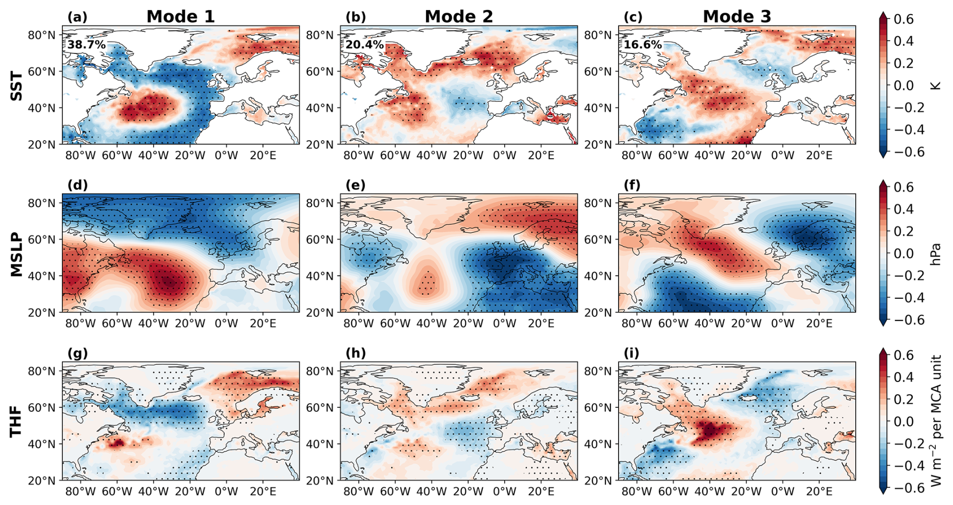
Figure 1 Contemporaneous autumn atmosphere-ocean co-variability in ERA5. Heterogeneous patterns for MCA modes 1–3 are shown for autumn SST (a–c), autumn MSLP (d–f), and autumn THF regressed onto the corresponding MCA timeseries (r(THF; MCA score)) (g–i). The percentage of squared covariance explained by each mode is shown in the legend in panels (a)–(c). Stippling indicates where the relationship is significant at the 5 % level.

Positive SST anomalies in MCA2 are exhibited across the subpolar north Atlantic, Labrador Sea and east of Canada accompanied by negative SST anomalies west of Europe (Fig. 1b). The associated MSLP anomalies (Fig. 1e) exhibit negative anomalies over the eastern North Atlantic, western Europe and North Africa and positive anomalies over Scandinavia, Greenland and a small region in the western part of the basin. Similar to MCA1, the THF regression pattern for MCA2 is anticorrelated with the SST anomalies (Fig. 1h).

In MCA3 there is a tripolar SST pattern with a band of warm anomalies extending from the Canadian coast to Portugal and cold anomalies to the east of the USA and surrounding Iceland and the UK (Fig. 1c). Positive MSLP anomalies are broadly collocated with positive SST anomalies with a slight northward phase shift of the wave train, and THF and SST anomalies are anticorrelated (Fig. 1f, i).

Figure 2 shows the CMIP6 multi-model mean MCA modes 1–3 of autumn SST (Fig. 2a–c) and autumn MSLP (Fig. 2g–i). The inter-model standard deviation of the MCA modes are shown in Fig. 2d–f for SST and Fig. 2j–k for MSLP. The modes for the individual models are shown in Figs. S3–S16. Each ensemble member covers the same 1940–2014 period as ERA5 and MCA is applied to each member individually before averaging. The spread across ensemble members therefore represents the sampling distribution of MCA patterns obtained from a 75-year record. Hatching denotes where the ERA5 MCA amplitude exceeds the 97.5th percentile of the distribution of all model ensemble members, and equivalently falls below the 2.5th percentile for stippling. The spatial structure of MCA modes 1–3 of the autumn SST-MSLP relationships are, on average, well captured by the models. ERA5 lies within the ensemble spread at most gridpoints, which means individual members can produce autumn SST MCA patterns that are locally as strong as ERA5. The inter-model spread indicates strong agreement among the models on the structure of MCA1, with small regions where the spread exceeds the multi-model mean mostly in areas where the amplitudes are weak in both ERA5 and the models (Fig. 2d, j, p). The inter-model spread is relatively larger for MCA modes 2 and 3, mainly regarding the position of the nodes between centres of action but this spread is still proportionately small compared with the multi-model mean and the overall patterns are generally consistent across models (Figs. S3–S16).

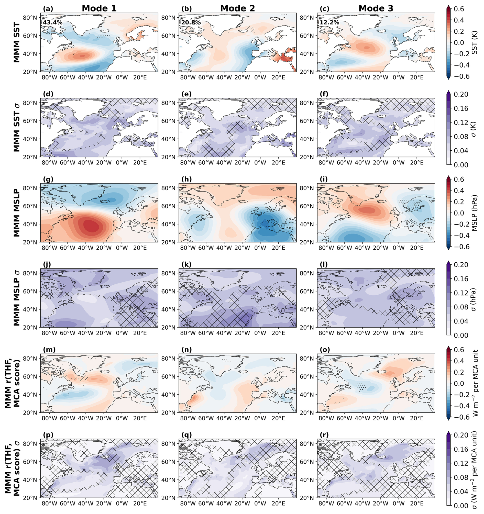
Figure 2 Multi-model mean (MMM) contemporaneous autumn atmosphere-ocean co-variability. Heterogeneous patterns for MCA modes 1–3 for autumn SST, autumn MSLP, and autumn turbulent heat flux (THF) regressed onto the corresponding MCA time series (r(THF, MCA score)). Panels are arranged left-to-right by mode (columns: Mode 1–3) and top-to-bottom by variable: (a–c) MMM SST, (d–f) inter-model spread in SST, (g–i) MMM MSLP, (j–l) inter-model spread in MSLP, (m–o) MMM r(THF, MCA score), and (p–r) inter-model spread in r(THF, MCA score). Hatching indicates regions where the ERA5 value exceeds the 97.5th percentile of the ensemble spreads, and stippling indicates regions where ERA5 falls below the 2.5th percentile of the ensemble spreads. Cross-hatching in panels (d)–(f), (j)–(l) and (p)–(r) indicate where the inter-model spread is greater than the multi-model mean. The mean percentage of squared covariance explained by each mode is shown in the legend in panels (a)–(c).

3.1.2 Relationship of autumn MCA modes with univariate EOFs

MCA identifies patterns that maximise covariance between two variables, which may be distinct from the dominant modes of variability of the separate variables. Figure 3 shows the Pearson correlation coefficient between the MCA1 timeseries and PCs 1–3 of each variable, to quantify the similarity between the MCA1 patterns and the separate EOFs 1–3 of SST and MSLP. The autumn SST and MSLP EOFs 1–3 are shown in Figs. S17 and S1 for comparison. We focus on MCA1 because this explains the largest proportion of SST and MSLP covariance.

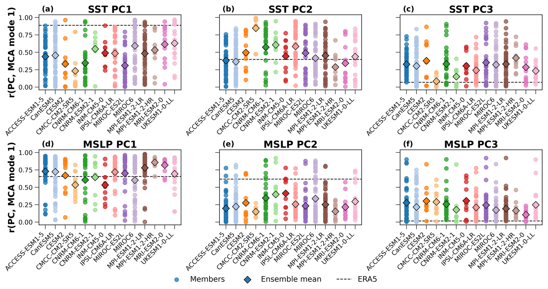
Figure 3 Correlation of autumn coupled variability and dominant modes of SST and MSLP. Correlation of the autumn MCA timeseries with autumn SST PCs (a–c) and autumn MSLP PCs (d–f). Circles are model members, diamonds are ensemble means and the dashed lines represent ERA5.

In ERA5, MCA1 SST primarily resembles EOF1 (r = 0.89, p = 1.3 × 10⁻²³), with a dominant warm anomaly in the central North Atlantic. The ERA5 correlation of SST MCA1 with EOF2 is weaker but significant (r = 0.40, p = 1 × 10⁻³) and insignificant for EOF3. In comparison with models, the ERA5 correlation between SST MCA1 and EOF1 lies in the extreme upper tail of the distribution of correlations across individual ensemble members for most models, generally above the 90th percentile (Fig. 3a). The correlation of SST MCA1 with PC2 lies well within the distributions of modelled correlations (Fig. 3b), while for PC3 the ERA5 correlation falls in the lower tail of the modelled distributions (Fig. 3c). This suggests that the modelled MCA1 SST anomalies do not resemble PC1 strongly enough and resemble PC3 more than in ERA5. However, in most cases, the ERA5 values lie within the spread of ensemble members meaning we cannot rule out that the reanalysis period was unusual. The exceptions are CMCC-CM2-SR5, CNRM-ESM2-1 and MIROC-ES2L where the MCA1 correlation with PC1 of SST is lower than in ERA5.

The autumn MSLP MCA1 in ERA5 is similarly correlated with MSLP PC1 (r = 0.66, p = 1.7 × 10⁻⁹) and PC2 (r = 0.62, p = 2.4 × 10⁻⁸). This means the autumn MCA1 resembles a mixture of EOF1 (Fig. S1a) and EOF2 (Fig. S1b), respectively. The ERA5 correlations of MSLP MCA1 with PC1 and PC2 lie within the spread of members for almost all CMIP6 models (Fig. 3d and e), indicating they are capable of capturing the resemblance of the MSLP MCA1 pattern to the separate MSLP EOFs. However, in all the models the resemblance of MCA1 to EOF3 is generally higher than in ERA5 and is comparable to that for the EOF2, indicating the MCA1 MSLP pattern is generally more of a mixture across different EOFs.

The analysis in this section has shown that the CMIP6 models simulate consistent covariability between SST, THF and MSLP in autumn to that found in ERA5, and that, after accounting for sampling uncertainty, the modelled MCA1 modes show consistent resemblance with the leading EOFs of each variable as in ERA5. Correlation analysis shows that MCA1 primarily corresponds to EOF1 of SST and EOF1 and 2 of MSLP, indicating that the coupled mode reflects large-scale variability patterns such as the NAO. Models capture these relationships, although they show a more variable representation of the relative similarity to each EOF compared to ERA5.

Lastly, we note that the analogous contemporaneous winter SST-MSLP MCA1 mode for ERA5 shows a tripolar SST structure (Fig. S18a) coupled with an NAO-like MSLP pattern (Fig. S18d). The winter THF anomalies associated with MCA1 are anticorrelated with SST (Fig. S18g), consistent with the autumn results. The CMIP6 models show similar contemporaneous winter MCA modes to ERA5 (Fig. S19), although some differences are evident. The band of positive SST anomalies extending from the Gulf Stream towards western Europe is weaker in the multi-model mean than in ERA5, with ERA5 anomalies lying beyond the 97.5th percentile of ensemble members (Fig. S19a) and the inter-model spread is larger in winter than in autumn.

This analysis provides a baseline for the remainder of the paper, as differences between model and ERA5 relationships in the lagged relationships are unlikely to arise from errors in atmospheric forcing of SST or in the dominant SST variability.

3.2 North Atlantic autumn to winter atmosphere–ocean covariability

3.2.1 Representation of autumn-winter MCA modes 1–3

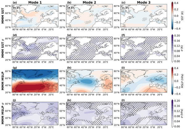
To investigate the potential effect of North Atlantic SST on the atmosphere, as discussed in Sect. 1, we next analyse the lagged MCA modes between autumn SST and winter MSLP. In ERA5, MCA1 explains 58 % of the squared covariance and is characterised by a positive SST anomaly in the central North Atlantic and negative anomaly in the tropical Atlantic and west of the UK and the Iberian peninsula (Fig. 4a), and a positive NAO-like MSLP pattern (Fig. 4d). The MCA1 SST pattern closely resembles that reported in Kolstad and O'Reilly (2024) for November SSTs, so this result supports their finding. MCA2 and MCA3 explain substantially less covariance in ERA5 compared with MCA1 (14 % and 8 %, respectively). Note that the colour bars are different from the contemporaneous autumn MCA modes in Figs. 1 and 2, highlighting that the lagged relationships are weaker.

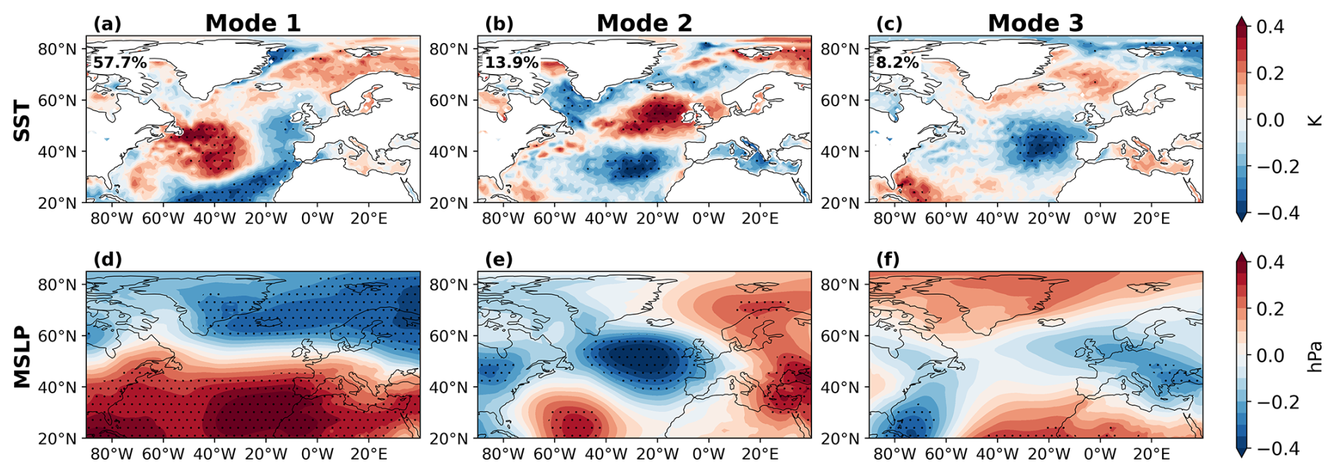
Figure 4 Lagged autumn-winter atmosphere-ocean co-variability in ERA5. Heterogeneous patterns for MCA modes 1–3 are shown for autumn SST (a–c) and winter MSLP (d–f). Percentage of squared covariance explained by each mode is given in the legends of panels (a)–(c). Stippling indicates where the relationship is significant at the 5 % level.

The corresponding multi-model mean lagged MCA1 autumn SST and winter MSLP patterns are shown in Fig. 5, along with the inter-model spread. The modes for individual models are shown in Figs. S20–S33. The multi-model mean MCA1 MSLP pattern shows an NAO-like structure (Fig. 5d), similar to ERA5. The inter-model spread in MCA1 MSLP near the dominant centres of action is small compared with the mean amplitude, indicating broad agreement among models of this pattern. The modelled MCA2 and MCA3 MSLP patterns also show strong agreement with ERA5, with the main centres of action being well captured (Fig. 5h, i).

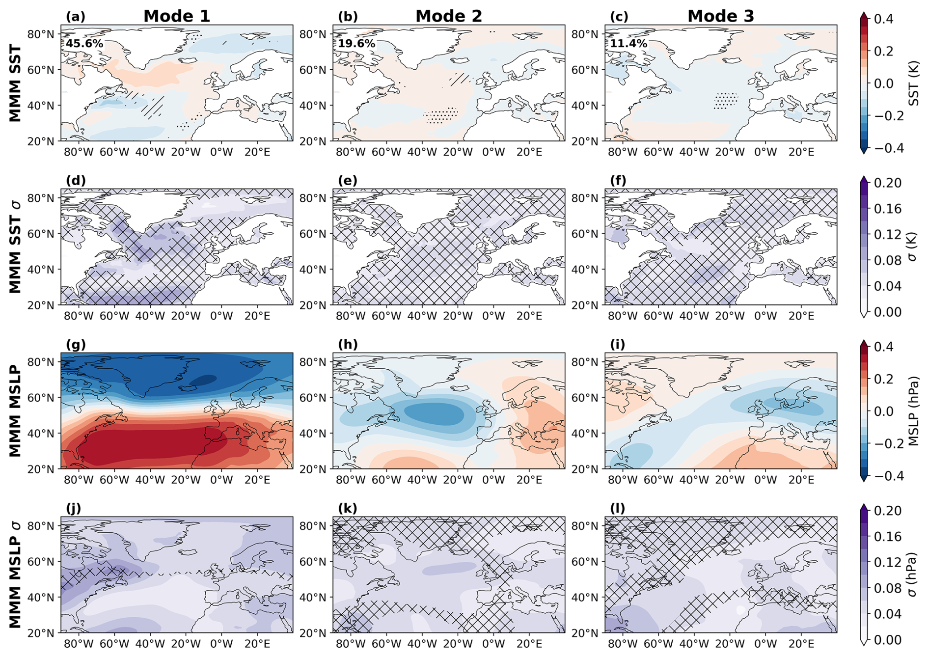
Figure 5 Multi-model mean lagged autumn-winter atmosphere-ocean co-variability. Heterogeneous patterns for MCA modes 1–3 are shown for autumn SST and winter MSLP. (a–c) MMM SST, (d–f) inter-model spread in SST (σ), (g–i) MMM MSLP, (j–l) inter-model spread in MSLP (σ). Hatching indicates regions where the ERA5 value exceeds the 97.5th percentile of the ensemble spread, and stippling indicates regions where ERA5 falls below the 2.5th percentile of the ensemble spread. Cross-hatching in panels (d)–(f), (j)–(l) and (p)–(r) indicate where the inter-model spread is greater than the multi-model mean. The mean percentage of squared covariance explained by each mode is shown in the legend in panels (a)–(c).

In contrast, the multi-model mean MCA1 SST pattern is markedly different from ERA5 both in amplitude and structure (Fig. 5a), and shows poor model agreement (Fig. 5d). This is similar for the SST patterns associated with MCA2 and MCA3, where the inter-model spread exceeds the multi-model mean amplitude (Fig. 5e–f). Despite the apparent differences between the modelled MCA SST patterns and ERA5, there are relatively few regions where ERA5 exceeds the 2.5th or 97.5th percentiles of the ensemble member spread (Fig. 5a–c), which is indicative that strong autumn SST MCA patterns can be found in individual members. The autumn-winter MCA SST patterns show more regions where ERA5 lies outside of the ensemble spread in individual models (Fig. S20–S33) for MCA1–3 where the main centres of action are either underestimated or have the opposite sign to ERA5.

The area averaged MCA1 autumn SST amplitude over the central North Atlantic region was computed for each ensemble member (Fig. S34). The ERA5 amplitude exceeds every member in 9 of 14 models. Across all models, only 5 ensemble members out of 371 have a lagged MCA1 autumn SST amplitude in the central North Atlantic equal to or greater than that in ERA5. The difference in the autumn SST precursor is therefore unlikely to be explained by sampling uncertainty alone.

3.2.2 Relationship of autumn-winter MCA modes with univariate EOFs

To quantify the similarity between the autumn SST-winter MSLP MCA1 and the separate EOFs for each variable, Fig. 6 shows the Pearson correlation coefficient between the MCA1 timeseries and PCs 1–3. The corresponding EOFs of autumn SST and winter MSLP in ERA5 and the CMIP6 models are shown in Figs. S17 and S2. As previously discussed, MCA1 MSLP predominantly resembles the winter NAO (EOF1) for ERA5 and the CMIP6 models (Fig. 6d), with weak correlations with PC2 and PC3 of winter MSLP (Fig. 6e–f). In contrast, in ERA5 the autumn-winter MCA1 SST shows the strongest correlation with PC1 (r = 0.92, p = 6.8 × 10⁻²⁹), with a value above the range of ensemble members for most models and in the very edge of the distribution for only three models (Fig. 6a). Conversely, the models show a stronger relationship of MCA1 with PC2 and PC3 of autumn SST than is seen in ERA5, which lies at the lower end of the ensemble member distributions for both PCs.

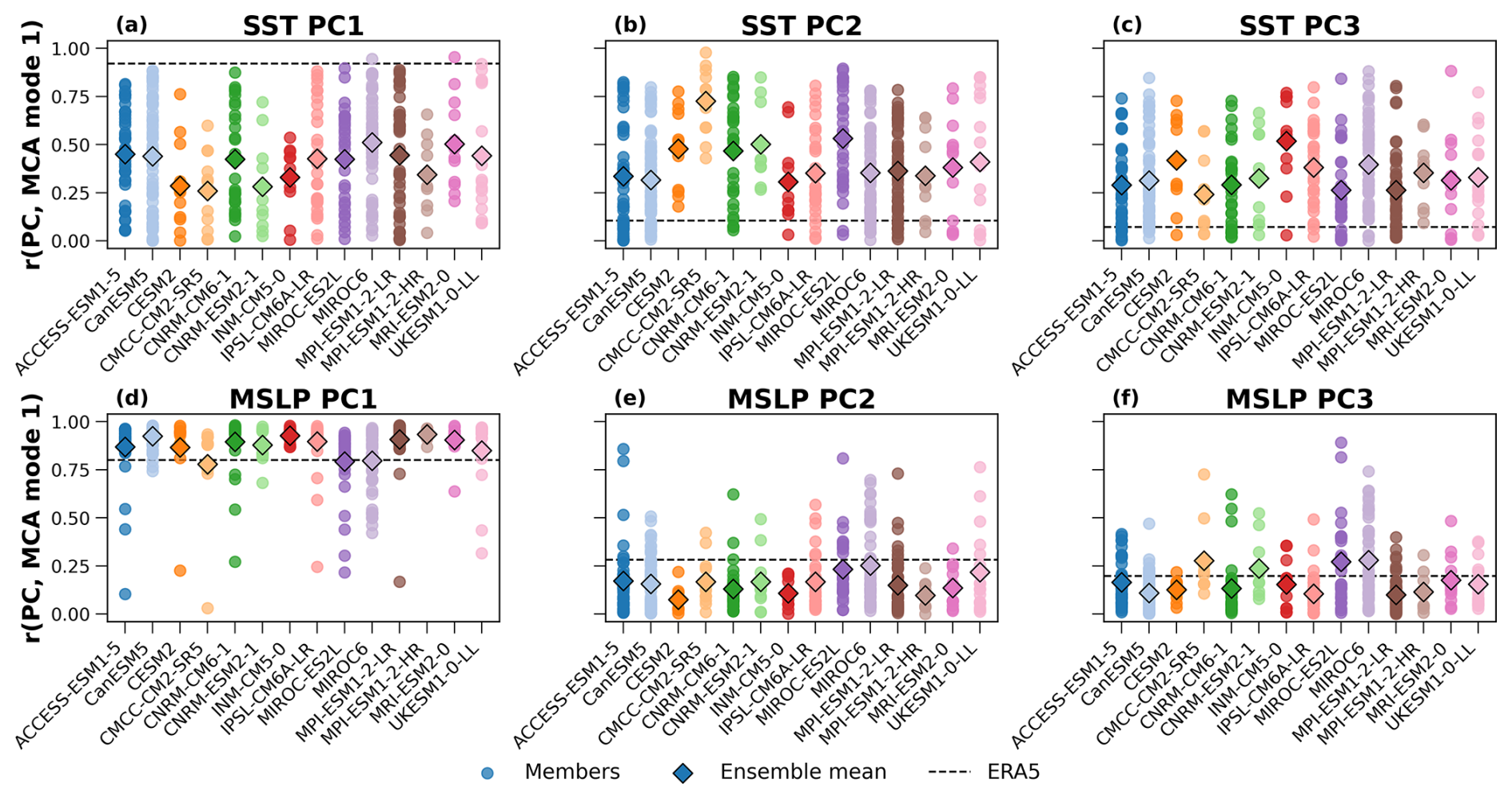
Figure 6 Correlation of autumn-winter coupled variability and dominant modes of SST and MSLP. Correlation of the autumn-winter MCA timeseries with autumn SST PCs (a–c) and winter MSLP PCs (d–f). Circles are model members, diamonds are ensemble means and the dashed lines represent ERA5.

These results show that the modelled covariance between autumn SST and winter MSLP appears to be different from ERA5. While ERA5 predominantly identifies PC1 of autumn SST as being related to the winter NAO, the models have a more mixed autumn SST signal which projects similarly onto EOFs 1–3 with no dominant preferred mode. This does not appear to be related to a systematic difference in the model representation of the EOFs of autumn SST or the relative variance explained by each mode (Fig. S17).

The lagged MCA cannot establish whether the ERA5 relationship reflects a feedback of the ocean onto the atmosphere. One possible explanation for the weaker lagged relationship in the models is that precursor autumn SST anomalies persist less strongly into winter than in ERA5. Figure 7 shows the regression of monthly SST anomalies for December, January and February onto the autumn SST-MSLP MCA1 expansion coefficients in the models and ERA5. We use the autumn MCA1 patterns because these are similar between the models and ERA5 (Figs. 1a and 2a), and they resemble the lagged autumn SST–winter MSLP MCA1 pattern in ERA5 (Fig. 4a), unlike the equivalent lagged MCA1 patterns in the models (Fig. 5a). The autumn SST pattern persists into winter in ERA5 and the models and the ERA5 regression lies within the 2.5–97.5th percentile range of all ensemble members over most of the North Atlantic. This result suggests that the weaker lagged autumn SST-winter MSLP relationship in the models cannot be attributed to weaker persistence of North Atlantic precursor SST anomalies.

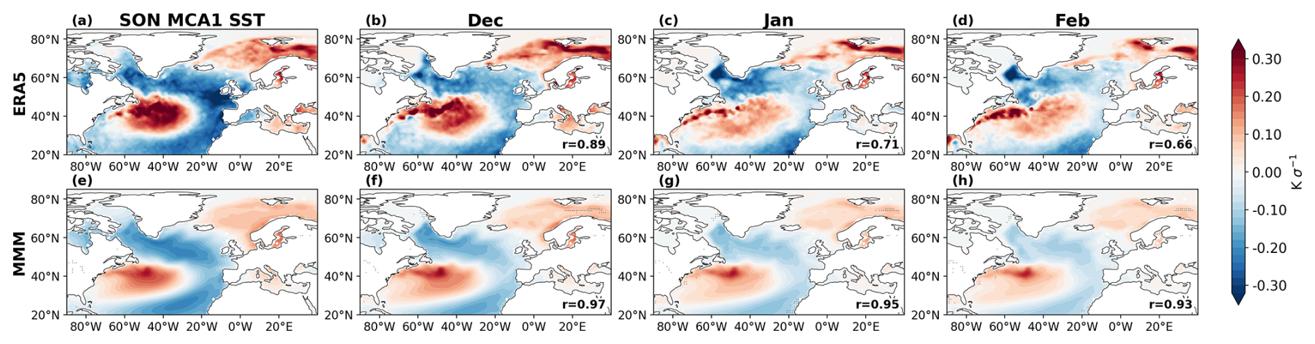
Figure 7 Persistence of the SON MCA1 SST pattern in ERA5 and models. Regression of December, January and February SST anomalies onto the SON MCA1 SST expansion coefficients in ERA5 and the MMM. The spatial correlation with the SON MCA1 SST pattern is shown by the r value in the bottom right corner of each plot. Stippling in panels (e)–(h) indicates where the ERA5 regression is outside of the 2.5–97.5th percentile range for all members.

Section 3.1 showed that autumn SST anomalies are largely generated by atmospheric forcing. A lagged covariance could therefore equally arise from persistence of an atmospheric anomaly into winter, or from a remote driver that forces both seasons. To distinguish between these possibilities, we separate the part of autumn air-sea heat exchange driven by the atmosphere from the part driven by the ocean.

3.3 Separating atmosphere and ocean-driven lagged autumn-winter variability

3.3.1 Decomposition of atmosphere and ocean drivers using analogues

The atmospheric circulation analogue method described in Sect. 2.3.3 was used to derive autumn THF anomalies associated with atmospheric forcing (THF_circ) and a residual, ocean-driven, component (THF_res). Following Patterson et al. (2024), the two leading EOFs of THF_circ and THF_res were calculated and the winter MSLP anomalies then regressed onto PC1 and PC2 of each THF component. While Patterson et al. (2024) focused on PC1, we include PC1 and PC2 because the two modes explain similar amounts of variance in the THF components. The result gives the winter MSLP anomalies that co-vary with the autumn THF, THF_circ and THF_res.

Figure 8 displays the patterns for ERA5. For PC1 and PC2, the spatial structure of the autumn THF and THF_circ are very similar (Fig. 8a, b, g, h), which shows that the atmospheric forcing dominates the spatio-temporal variance of North Atlantic THF in autumn.

There is a strong resemblance between PC1 of THF and THF_circ in ERA5 (Fig. 8a, b) and the THF regressed onto MCA1 of autumn SST and MSLP (Fig. 1g), which is coincident with an autumn MSLP MCA1 pattern that projects similarly onto the NAO and EAP (Fig. 3d, e). However, the MSLP anomalies regressed onto PC1 of THF and THF_circ (Fig. 8d, e) are distinct from one another and do not resemble any single EOF, suggesting less coherent atmospheric spatio-temporal persistence from autumn into winter associated with PC1.

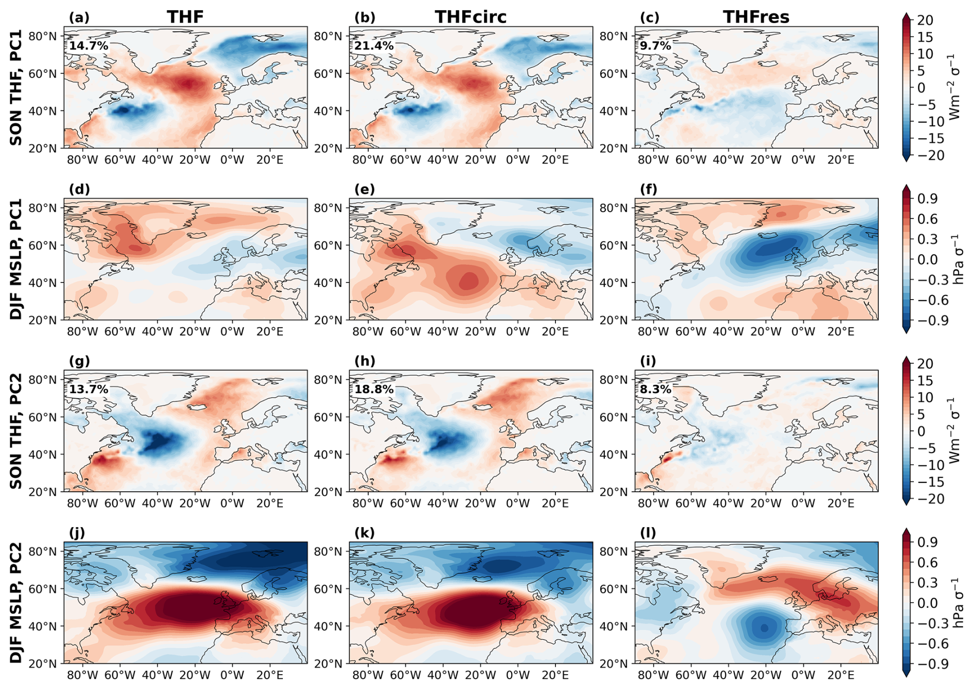
Figure 8 Relationships of THF and MSLP with components of THF decomposition in ERA5. Regression of autumn THF and winter MSLP onto PC1 (a–f) and 2 (g–l) of total THF, THF_circ and THF_res. Variance explained by PC1 and PC2 of each THF component is shown in the legend in panels (a)–(c) and (g)–(i), respectively.

There is also resemblance between PC2 of THF and THF_circ in ERA5 (Fig. 8g, h) and THF regressed onto MCA3 for contemporaneous autumn SST and MSLP covariance in ERA5 (Fig. 1i). The corresponding autumn MSLP pattern associated with MCA3 resembles a Rossby wave train emanating from the tropical Atlantic which is similar to EOF2 of autumn MSLP, but with a phase shift of about half a wavelength (compare Fig. 1f and Fig. S1). In contrast, the regression of winter MSLP onto PC2 of autumn THF and THF_circ in ERA5 shows a positive NAO pattern (Fig. 8j, k). Together, these results suggest that in ERA5, the second leading mode of autumn THF variability is linked with atmospheric forcing connected to a tropically-forced Rossby wave train, and the same forcing may also contribute to winter NAO variability independent of autumn ocean-driven THF_res.

We now consider the signals associated with ocean-driven autumn THF variability. PC1 of autumn THF_res shows broad negative anomalies in the Gulf Stream region extending with a north-eastward tilt across the basin and positive THF_res anomalies at higher latitudes (Fig. 8c). The winter MSLP anomalies associated with PC1 of THF_res resemble any of EOF2 of winter MSLP (compare Fig. 8f and Fig. S2).

In PC2 of THF_res, there is a negative THF anomaly in the central North Atlantic and a positive anomaly in the Caribbean Sea and the southern flank of the Gulf Stream (Fig. 8i), which do not strongly resemble any of the THF anomaly patterns associated with autumn MCA1-3 (Fig. 1g–i). The winter MSLP regression onto PC2 of autumn THF_res is markedly different from THF and THF_circ and does not closely resemble the dominant EOFs of winter MSLP (compare Fig. 8f and Fig. S2).

The magnitude of winter MSLP anomalies associated with PC1 and PC2 of autumn THF_res is generally weaker than for THF and THF_circ. These results suggest that in ERA5 winter NAO variability is partly related to autumn atmosphere-driven THF anomalies, but is not related to ocean-driven autumn THF anomalies.

3.3.2 Sampling uncertainty in isolating atmosphere and ocean drivers

To examine sampling uncertainty, Fig. 9 shows the projection of the winter MSLP regression onto PC2 of autumn THF, THF_circ and THF_res onto the winter NAO for ERA5 and the CMIP6 models. R² is the fraction of the variance in the MSLP regression pattern explained by the NAO, and c is the magnitude of the associated NAO index anomaly. These metrics quantify the extent to which autumn THF, THF_circ and THF_res variability correlates with the winter NAO. The individual ensemble member points provide information about the sampling uncertainty in the models. For ERA5, sampling uncertainty was assessed by bootstrapping without replacement the years used to compute the THF EOFs with a bootstrap sample size of N = 40.

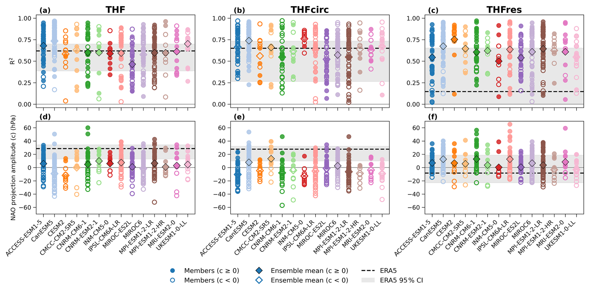
Figure 9 Projection of the regression pattern of winter North Atlantic MSLP onto PC2 of the autumn THF components onto the winter NAO (EOF1) in ERA5 and models. Fraction of the variance explained by the NAO (a–c) and strength of the NAO signal (d–f). Circles are model members, diamonds are ensemble means, dashed black lines represent ERA5, grey shading represents the sampling uncertainty. Positive c values indicate a positive NAO and negative indicate a negative NAO.

For PC2 of THF and THF_circ, there is a robust projection onto the NAO in ERA5 and the CMIP6 models (Fig. 9a, b). We note that although the pattern correlations are similar between ERA5 and the models, the winter NAO index anomaly associated with autumn THF and THF_circ variability lies in the upper tail or outside of the ensemble spread in every model (Fig. 9d, e). Since this is the component of THF driven by autumn atmospheric forcing, this could imply there are issues with modelled atmospheric persistence or teleconnections that serve as a common forcing of the autumn and winter atmosphere. While the models show a stronger resemblance of the MSLP pattern associated with PC2 of THF_res than the near-zero anomaly in ERA5 (Fig. 9c), the magnitude of the associated NAO index anomaly is substantially smaller than for THF and THF_circ (Fig. 9f) suggesting this makes a small contribution to winter NAO variability.

The sampling uncertainty for all THF components is large, with the ensemble spread in R² spanning a large range from near-zero to almost 1 in many models and the NAO index anomaly spanning positive and negative values. The sampling uncertainty in ERA5 is also substantial, but as expected less than the ensemble spread given the uncertainty is estimated using bootstrapping rather than different samples as in the ensemble members. This uncertainty highlights the challenge of estimating small signals in the winter atmospheric circulation which is influenced by myriad remote drivers and large internal atmospheric variability. Accounting for the sampling uncertainty in ERA5, the results reveal no systematic biases in the modelled relationships of winter MSLP with autumn THF_circ. An equivalent analysis based on PC1 of the THF components is shown in Fig. S36.

The circulation analogue decomposition has shown that autumn North Atlantic THF variability is primarily controlled by atmospheric forcing, with limited evidence for an influence of ocean-driven autumn THF anomalies on the winter NAO. The ocean driven component is associated with weak winter MSLP anomalies that do not project onto the NAO. The previously identified autumn–winter NAO relationship in ERA5 is therefore not explained by ocean-driven THF anomalies.

The models capture the pattern of the THF_circ–winter NAO relationship, but underestimate its magnitude. The winter NAO signal linked to THF_circ could reflect SST anomalies that are forced by the autumn atmosphere and then persist and feedback later. Alternatively, it could reflect a common remote driver acting on both seasons. The analogue method cannot separate these, as it attributes all circulation related THF to THF_circ.

4 Discussion and Conclusions

This study evaluated whether CMIP6 large ensembles reproduce the observed relationship between autumn North Atlantic SST anomalies and the subsequent winter atmospheric circulation. The results show that atmospheric forcing of the ocean, seen in contemporaneous co-variability, is well represented. In contrast, the lagged relationship, which is where an ocean influence on the atmosphere would be expected to appear, differs substantially between ERA5 and models. These differences are consistent with atmospheric GCM experiments, in which the atmospheric response to extratropical SST anomalies is small relative to internal variability and strongly model dependent (Kushnir et al., 2002).

The close agreement between ERA5 and the multi-model mean in the spatial structure of the leading MCA modes (Figs. 1 and 2), suggests that climate models realistically represent contemporaneous atmosphere-ocean co-variability in autumn and winter, when atmospheric forcing dominates THF and SST variability. The anti-correlation between SST and THF anomalies, together with the NAO-like structure of MSLP, is consistent with a short timescale ocean response to atmospheric forcing via wind-driven turbulent heat fluxes (Cayan, 1992; Marshall et al., 2001; Czaja and Frankignoul, 2002).

The seasonal transition from a horseshoe SST pattern in autumn (Fig. 2a) to a tripolar structure in winter (Fig. S19a) reflects a shift in the dominant modes of variability and is consistent with the NAO forcing of SSTs in winter (Deser and Timlin, 1997; Marshall et al., 2001). Some differences between ERA5 and the models emerge in winter, particularly the weaker SST anomalies in the eastern north Atlantic (Fig. S19a), which may be related to the apparent westward shift in the Azores High in the models. The larger inter-model spread in winter is consistent with the increased variability of both SST and MSLP during this season.

The relationship between the leading MCA mode and the dominant modes of SST and MSLP variability provides further insight into model performance. In ERA5, the autumn MCA1 mode is strongly correlated with SST EOF1 (Fig. 3a), confirming that the primary coupled mode reflects large-scale SST variability. The associated MSLP pattern projects onto MSLP EOF1 and 2 in ERA5 (Fig. 3d, e), indicating that the coupled variability represents a combination of atmospheric modes. CMIP6 models show similar correlation of the MCA1 SST anomalies with SST EOF1, but a weaker correlation of MCA1 MSLP anomalies with MSLP EOF2. This difference suggests that models may underestimate the contribution of this mode to the coupled variability, which may influence how SST anomalies respond to atmospheric forcing. This could be linked to biases in the drivers of this mode including large-scale teleconnections, such as those associated with ENSO (e.g. Maidens et al., 2021; Thornton et al., 2023). Overall, the results indicate that while models capture the primary features of atmosphere-ocean coupling in autumn and winter, there are differences in the relative importance of different atmospheric modes.

In contrast to the strong agreement in contemporaneous atmosphere–ocean relationships in autumn and winter seasons, the representation of lagged autumn–winter coupling is notably weaker in the models. Although ERA5 and the models show a winter NAO-like anomaly for MCA1 (Figs. 4d and 5g), the associated autumn SST precursor pattern differs substantially. In ERA5, the autumn SST associated with the lagged MCA1 is characterised by a central North Atlantic SST anomaly that closely resembles EOF1 of autumn SST variability (Fig. 4a). However, in the models, the autumn SST precursor exhibits no consistent structure and shows large inter-model spread, with ERA5 lying outside the ensemble range in key regions (Fig. 5a). This difference indicates that the models generally underestimate the connection between EOF1 of autumn SST and the winter NAO. This is consistent with previous work showing that the covariance between North Atlantic SST anomalies and the NAO is weaker in climate models than in observations (Bonnet et al., 2024; Patrizio et al., 2025).

Given that the leading modes of autumn SST variability are well represented in the models (Fig. S17) this discrepancy is unlikely to arise from the SST field itself and the persistence of the winter NAO precursor autumn SST anomalies into the winter is also comparable between the models and ERA5 (Fig. 7). The decomposition of THF provides additional insight into the mechanisms underlying this lagged relationship. The similarity of the variability in THF and the atmosphere-driven component (THF_circ) indicates that interannual autumn THF variability is primarily controlled by atmospheric forcing (Fig. 8a–b, g–h). The PC2 of THF and THF_circ project onto a winter NAO pattern (Fig. 8j, k). In contrast, regression of winter MSLP onto the ocean-driven component THF_res results in anomalies that do not project onto the NAO (Fig. 8l). This result suggests that the component of autumn ocean variability that is independent of contemporaneous atmospheric circulation exerts only a weak influence on the winter atmosphere including the NAO. The resemblance of the lagged winter MSLP anomalies associated with all autumn THF components exhibits large sampling uncertainty, indicating the winter atmospheric circulation is highly variable and detecting a relatively small signal associated with autumn THF precursors is challenging.

Within the circulation analogue framework applied here, any variability that projects onto large-scale atmospheric circulation patterns is attributed to the atmosphere-driven component. Consequently, any SST anomaly that is forced by atmospheric variability, such as those identified in the contemporaneous autumn MSLP-SST MCA modes, will be absent from THF_res and included in THF_circ. Therefore, it is possible that autumn SST anomalies driven by THF_circ could persist into the winter and contribute to anomalous THF at a later time that generates a lagged NAO anomaly. This could arise from a meridional temperature gradient feedback, in which the NAO cools the sub-polar gyre increasing the meridional temperature gradient and further increasing the NAO. Further investigation of this is left for future work. As the models reproduce the persistence of these SST anomalies into winter (Fig. 7), any model deficiency in this pathway would have to lie in the atmospheric response to the persisting SST anomalies rather than in the persistence itself. This could be consistent with the findings of Kolstad and O'Reilly (2024) where SST anomalies are treated as predictors and their influence on the atmosphere is assessed through intermediate variables such as THF and baroclinicity. An alternative explanation is that another remote driver generates atmospheric teleconnections in both autumn and winter, which creates the atmospheric forcing that drives autumn THF/SST and the subsequent winter NAO anomaly independent of a feedback from North Atlantic SST onto the atmosphere. An example could be ENSO, which produces an EAP-like anomaly in autumn and an NAO-like anomaly in winter (e.g., Ayarzagüena et al., 2018). More generally, remote tropical forcing can drive lagged relationships between North Atlantic SST and atmospheric variability without requiring a direct causal influence of local SST anomalies (Czaja and Frankignoul, 2002; Maidens et al., 2021). Under this interpretation, the observed autumn SST anomalies reflect the atmospheric response to a common remote forcing, rather than acting as a driver of the subsequent winter circulation. Such an explanation would contrast the interpretation of local North Atlantic SST anomalies having a significant causal influence on the winter NAO on seasonal timescales through delayed air-sea feedbacks. Another possible pathway for autumn-winter covariability could involve the stratosphere if an autumn teleconnection drives THFcirc and also affects the stratospheric polar vortex leading to an NAO signal in winter (e.g., Ineson and Scaife, 2009).

Clarifying which of these hypotheses can explain the apparent autumn-winter relationship would be a useful contribution of future studies. Overall, the results show that climate models capture the key features of contemporaneous North Atlantic atmosphere-ocean coupling in autumn and winter. However, the models show weaker lagged relationships between autumn SST anomalies and subsequent winter atmospheric circulation compared to ERA5.