Understanding the contrasting environments for localised and widespread heavy rainfall in the tropics

Localised and widespread heavy rainfall cause different impacts and are increasingly recognised to be associated with different atmospheric regimes. Here we develop a simple model of a convective ensemble based on a spectrum of entraining plumes. The model relates both rainfall intensity and mean rainfall over the ensemble to the large-scale thermodynamic environment. According to this spectral plume model, widespread heavy rainfall occurs when the free-troposphere is relatively moist, whereas localised heavy rainfall occurs under a drier and more unstable troposphere. These results are confirmed using 20 years of weather radar observations and reanalysis data near Darwin, Australia. Further, using the connection between the convective environment and the entrainment distribution within the plume spectrum model, a bulk estimate of convective entrainment is diagnosed from the observational data. This estimate suggests that entrainment decreases with increasing boundary layer depth, but is largely independent of the size or organisation of convective rain cells. The analysis framework developed here is a useful tool for both diagnosing processes and evaluating high-resolution models.

1 Introduction

Precipitation is a multiscale phenomenon. Precipitation extremes occur across a range of spatial scales, from localised convective extremes that trigger hail and flash flooding to widespread systems that produce spatially extensive floods. Despite this, comparatively few observational studies of heavy precipitation explicitly consider the spatial characteristics of precipitation events (e.g., Louf et al., 2019; Bevacqua et al., 2021; Lin et al., 2026). Instead, precipitation is often characterised through an areal-mean over a fixed-size spatial domain in gridded observations (e.g., Yao et al., 2008; White et al., 2022; Angulo-Umana and Kim, 2023), or through effective point measurements provided by rain gauges (e.g., Alexander et al., 2006; Khouakhi et al., 2017; Risser et al., 2019).

While both such characterisations provide useful measures of precipitation intensity relevant to impacts and model evaluation, understanding the relationship between them depends on understanding how precipitation is organised spatially. In the tropics, it is well known that the organisation of convection plays an important role in determining the characteristics of heavy precipitation (e.g., Roca and Fiolleau, 2020; Moseley et al., 2016; Dai and Soden, 2020). Mesoscale convective organisation has been argued to enhance sub-daily areal-mean rainfall (Angulo-Umana and Kim, 2023) and daily extreme rainfall (Bao et al., 2024), while Louf et al. (2019) showed that larger convective cells, which they took to be more organised, tend to have higher radar-estimated rainfall intensity. But Louf et al. (2019) also found that the largest local rainfall intensities occur under different large-scale environments to those associated with the heaviest areal-average rainfall rates: intense local rainfall occurs in drier, subsiding environments, whereas heavy areal-mean rainfall occurs in moister, ascending environments. In the same vein, Hamada et al. (2015) showed that heavy precipitation and intense deep convection are not always co-located based on satellite observations. In idealised convection-permitting simulations, Singh et al. (2019) found that domain-mean precipitation increased with stronger large-scale ascent, while extreme updrafts were relatively insensitive to forcing strength and were not a simple function of instability. Combining observations and numerical simulations, Raymond et al. (2024) showed that the intense but localised “showers” tend to occur in drier but more unstable environments whereas the weaker but widespread “rains” are associated with very moist environments with weak instability. These studies highlight our lack of understanding of the physical factors controlling heavy rainfall at different spatial scales. In this work, we contrast locally intense rainfall and areal-averaged rainfall over a mesoscale-sized region. We develop a simple model that explains the differing relationships between both types of extremes and the large-scale thermodynamic environment, and we test this model using reanalysis and radar observations of rainfall near Darwin, Australia.

Understanding the relationships between convection and its environment is important for interpreting climate projections. Because the scales of processes involved in tropical convection are smaller than those represented by global climate models (∼ 150 km; Bao et al., 2024), large-scale environmental conditions have long been used as proxies to project changes in convection-related natural hazards in a warmer climate (e.g., Chen et al., 2020; Brown and Dowdy, 2021; Brooks, 2013). For example, models robustly project increases in convective available potential energy (CAPE) in the tropics (Singh et al., 2017; Chen et al., 2020) and many extratropical regions (e.g., Trapp et al., 2007; Brooks, 2013; Allen et al., 2014), suggesting increases in severe weather in the future (e.g., Allen et al., 2014; Diffenbaugh et al., 2013). However, CAPE represents an upper-bound on buoyancy-driven updraft kinetic energy and does not factor in the important effect of entrainment mixing (Peters et al., 2020a). The increase in convective intensity may therefore be substantially smaller than that implied by the increase in CAPE (Singh and O'Gorman, 2015). Several studies have incorporated entrainment to calculate entraining CAPE (ECAPE) and found that ECAPE predicts maximum updraft speed more accurately than conventional CAPE (Peters et al., 2022, 2023). Moreover, entrainment mixing provides a mechanism by which convection is sensitive to the humidity of its environment. This has been argued to be responsible for the well-known dependence of areal-average precipitation on column water vapour in the tropics (Bretherton et al., 2004; Ahmed and Neelin, 2018). Entrainment may also link convective intensity to vertical wind shear and the depth of the sub-cloud layer. Stronger shear has been argued to reduce fractional entrainment, thereby preserving more undiluted air within the convective cores (e.g. Peters et al., 2019, 2020b; Jo and Lasher-Trapp, 2022; Maybee et al., 2024); similarly, a higher lifting condensation level can favour wider updrafts and reduced fractional dilution (e.g. Mulholland et al., 2021; Takahashi et al., 2023; Peters et al., 2026). One aim of this paper is to understand the relative importance of (in)stability and humidity in environments associated with both local and areal-averaged heavy rainfall.

A challenge in relating convection to its environment is their two-way interactions, with convection not only driven by the large-scale environment but also shaping tropospheric temperature and humidity profiles (e.g., Arakawa and Schubert, 1974). Previous studies have derived the theoretical temperature perturbation profiles constrained by convection with and without entrainment (Yu and Neelin, 1997; Li et al., 2022). Singh and O'Gorman (2013) developed a theory for CAPE in the tropics assuming that convection maintains a lapse rate neutral to an entraining plume. The predicted relationship between humidity and instability in the troposphere is consistent with observational analyses (Palmer and Singh, 2024). However, the neutrality assumption does not allow one to reason directly about changes in convective buoyancy and intensity. For this purpose, a model with multiple plumes is needed (Singh and O'Gorman, 2015). Zhou and Xie (2019) derived a spectral plume model which predicts both CAPE and cloud buoyancy given an assumption about the distribution of entrainment rates within convection. Here, we build on this work and develop a similar model which provides a relationship between the convective mass flux of an ensemble of clouds and the large-scale thermodynamic environment.

The model is based on two assumptions: (1) convection is made up of a spectrum of plumes that each detrains at their level of neutral buoyancy (LNB), and (2) the entrainment rate of the plumes is set by a distribution of boundary-layer thermals that depends on the boundary-layer height. The model predicts that, consistent with previous observational studies (Ahmed and Neelin, 2018), areal-average precipitation increases as the atmosphere becomes moister and more unstable, allowing more plumes to be buoyant. The localised convective intensity, however, is primarily sensitive to the plumes with low entrainment rates, and it increases with instability and, for some measures, even decreases as the atmosphere becomes moister.

A key challenge in testing the above predictions is the limited spatial and temporal coverage of available observations. Gridded products and rain gauges are usually limited by the density of their observational networks and can only provide observations over land. Satellite observations provide broader spatial coverage but often lack the necessary spatial and temporal resolution to capture the rapidly evolving, localised convective systems. Compared with ground-based measurements, satellite-based products exhibit greater uncertainty in capturing precipitation magnitude (Alexander et al., 2020). Ground-based radar, while offering limited spatial coverage, provides high-resolution observations that are well suited for resolving the fine-scale structure of convection. Therefore, this study uses long-term (∼ 20 years) high spatial (1 km) and temporal (10 min) resolution radar observations in Darwin, Australia, to characterise the spatial characteristics of tropical rainfall.

By plotting solutions to the plume model and observed properties of convection in a phase space of environmental stability and humidity introduced by Palmer and Singh (2024), we show that the radar observations generally support the results of the plume model. Heavy precipitation is observed to occur under different combinations of stability and humidity depending on whether one considers the local intensity of convective cores or the mean rain rate across the radar domain. Morphological analysis further shows that higher CAPE is associated with fewer but larger convective cells and higher maximum convective cell intensity, along with more organised convection, in agreement with Louf et al. (2019). Consistent with previous studies (Zipser and LeMone, 1980; May and Ballinger, 2007; Yang, 2018; Peters et al., 2020a; Takahashi et al., 2021, 2023; Powell, 2024) and the plume model, the environments associated with heavy rainfall shift toward a more stable atmosphere when the boundary-layer height is high, implying a lower effective entrainment rate. Together, the plume model and the stability–humidity plane provide a new framework for examining the interaction between convection and its environment in models and observations alike.

This paper is structured as follows. Section 2 introduces the spectral plume model and the stability–humidity plane. Section 3 describes the weather radar and reanalysis data, and the methods used to characterise areal-mean precipitation, local intensity, and large-scale environmental conditions using these observations. Section 4 presents the observational results and comparison to the spectral plume model, followed by discussions and conclusions in Sect. 5.

2 A model for the relationship between convection and the large-scale environment

In this section, we develop a simple model of a convective ensemble based on the spectral plume model (SPM) of Zhou and Xie (2019) in order to relate the amount and intensity of convection to the mean thermodynamic profiles within a mesoscale region of the tropics. The model takes the areal-mean precipitation rate as an input, and it therefore does not provide a causal link between the total precipitation and the thermodynamic environment. Nevertheless, the SPM predicts that the largest area-mean precipitation rates and the most intense convective updrafts occur under different large-scale thermodynamic conditions, a prediction that is then tested using radar observations (Sect. 4).

2.1 Derivation of the spectral plume model (SPM)

Following the classic work of Arakawa and Schubert (1974), we consider the convective ensemble consisting of a spectrum of plumes with varying entrainment rates ϵ^′. The mass flux of each plume m(ϵ^′) increases with height z as it entrains and is governed by

$$\begin{array}{}\text{(1)}& {\displaystyle \frac{\mathrm{1}}{m}}{\displaystyle \frac{\partial m}{\partial z}}={\mathit{ϵ}}^{\prime }\end{array}$$

from the cloud base z_b up to its LNB, at which point it is assumed to detrain into the environment. We further assume that each plume is saturated above cloud base, and that the moist static energy of each plume h_p is governed by,

$$\begin{array}{}\text{(2)}& {\displaystyle \frac{\partial h_{\mathrm{p}}}{\partial z}}=-{\mathit{ϵ}}^{\prime }(h_{\mathrm{p}}-h_{\mathrm{e}}),\end{array}$$

where $h_{\mathrm{p}}=c_p(T-T_{\mathrm{0}})+gz+l_{\mathrm{v}\mathrm{0}}q$ and h_e is the moist static energy of the environment, defined analogously. Here T is the temperature, q is the specific humidity, c_p is the isobaric specific heat capacity of the dry air–vapour mixture, g is the gravitational acceleration constant, and l_v0 is the latent heat of vaporisation at a reference temperature T₀=273.15 K. For simplicity, we neglect any contribution of freezing to the moist static energy, and we assume no condensate (liquid or ice) is present in the parcel.

Since each plume within the spectrum has a different entrainment rate, it will become neutrally buoyant and detrain at a different level. Zhou and Xie (2019) showed that one could solve for h(z), the moist static energy of the plume that detrains at level z. Note that h(z) does not represent the vertical profile of any individual plume. Specifically, h(z) is approximately governed by the equation

$$\begin{array}{}\text{(3)}& {\displaystyle \frac{\partial h\left(z\right)}{\partial z}}-\mathit{\lambda }\left[h\left(z\right)-h\left(z_{\mathrm{b}}\right)\right]=-\mathit{ϵ}\left(z\right)\left[h\left(z\right)-h_{\mathrm{e}}\left(z\right)\right].\end{array}$$

Here ϵ(z) is the entrainment rate of the plume that detrains at level z and

$$\begin{array}{}\text{(4)}& \mathit{\lambda }={\displaystyle \frac{\mathrm{1}}{\mathrm{1}+\mathrm{0.75}\mathit{ϵ}\left(z\right)(z-z_{\mathrm{b}})}}{\displaystyle \frac{\mathrm{d}\ln \mathit{ϵ}}{\mathrm{d}z}},\end{array}$$

as defined in Zhou and Xie (2019).

Since h(z) refers to a plume at its LNB, we can relate its properties to those of the environment. Neglecting the effect of moisture on density, h(z) is equal to the saturation moist static energy of the environment $h_{\mathrm{e}}^{\ast }\left(z\right)$, and we may therefore write Eq. (3) entirely in terms of environmental quantities:

$$\begin{array}{}\text{(5)}& {\displaystyle \frac{\partial h_{\mathrm{e}}^{\ast }\left(z\right)}{\partial z}}-\mathit{\lambda }\left[h_{\mathrm{e}}^{\ast }\left(z\right)-h_{\mathrm{e}}^{\ast }\left(z_{\mathrm{b}}\right)\right]=-\mathit{ϵ}\left(z\right)l_{\mathrm{v}\mathrm{0}}\left(q_{\mathrm{e}}^{\ast }\left(z\right)-q_{\mathrm{e}}\left(z\right)\right),\end{array}$$

where q_e and $q_{\mathrm{e}}^{\ast }$ are the specific humidity and saturation specific humidity of the environment, respectively.

Given the tropospheric relative humidity RH and the entrainment rate of the plume detraining at each level ϵ(z), either Eq. (3) or Eq. (5) may be used to infer the saturation moist static energy of the environment, which we take to be that of the large-scale mean atmosphere. From this, one may derive the mean temperature and humidity profiles assuming hydrostatic balance.

Zhou and Xie (2019) assumed power-law profiles of ϵ(z), finding that their solutions compared well to simulations of radiative–convective equilibrium. Here, we instead relate ϵ(z) to the mass flux required to produce a given areal-mean precipitation rate, allowing us to explore how the thermodynamic structure of the atmosphere varies with precipitation.

At each level z, the total mass flux M(z) is given by a sum over all plumes that are positively buoyant:

$$\begin{array}{}\text{(6)}& M\left(z\right)=\underset{\mathrm{0}}{\overset{\mathit{ϵ}\left(z\right)}{\int }}m\left({\mathit{ϵ}}^{\prime }\right)\mathrm{d}{\mathit{ϵ}}^{\prime }.\end{array}$$

Using Eq. (1), this may be written in terms of the cloud-base mass flux distribution m_b(ϵ^′):

$$\begin{array}{}\text{(7)}& M\left(z\right)=\underset{\mathrm{0}}{\overset{\mathit{ϵ}\left(z\right)}{\int }}{m}_{\mathrm{b}}\left({\mathit{ϵ}}^{\prime }\right)e^{{\mathit{ϵ}}^{\prime }(z-z_{\mathrm{b}})}\mathrm{d}{\mathit{ϵ}}^{\prime }.\end{array}$$

The distribution m_b(ϵ^′) may be thought of as representing the spectrum of thermals in the boundary layer, a fraction of which are positively buoyant and may contribute to the free-tropospheric convective mass flux. As a simple starting point, we assume this distribution to be uniform: $m_{\mathrm{b}}\left({\mathit{ϵ}}^{\prime }\right)=M_{\mathrm{0}}/{\mathit{ϵ}}_{\mathrm{0}}$, where M₀ is the cloud-base mass flux required under the conditions of radiative–convective equilibrium, and ϵ₀ is a characteristic entrainment rate. Since the maximum size of boundary-layer thermals scales with the depth of the boundary layer and we expect larger thermals to lead to plumes with smaller entrainment rates (Morton et al., 1956), we set the characteristic entrainment rate ${\mathit{ϵ}}_{\mathrm{0}}=E/z_{\mathrm{b}}$, for a non-dimensional parameter E. Figure 1 shows m_b(ϵ^′) for different cloud-base heights and cloud-base mass fluxes. Buoyant plumes exist up to a maximum entrainment rate ϵ_b=ϵ(z_b). A higher cloud base results in a set of buoyant plumes limited to relatively small entrainment rates, while a larger cloud-base mass flux implies a wider entrainment distribution.

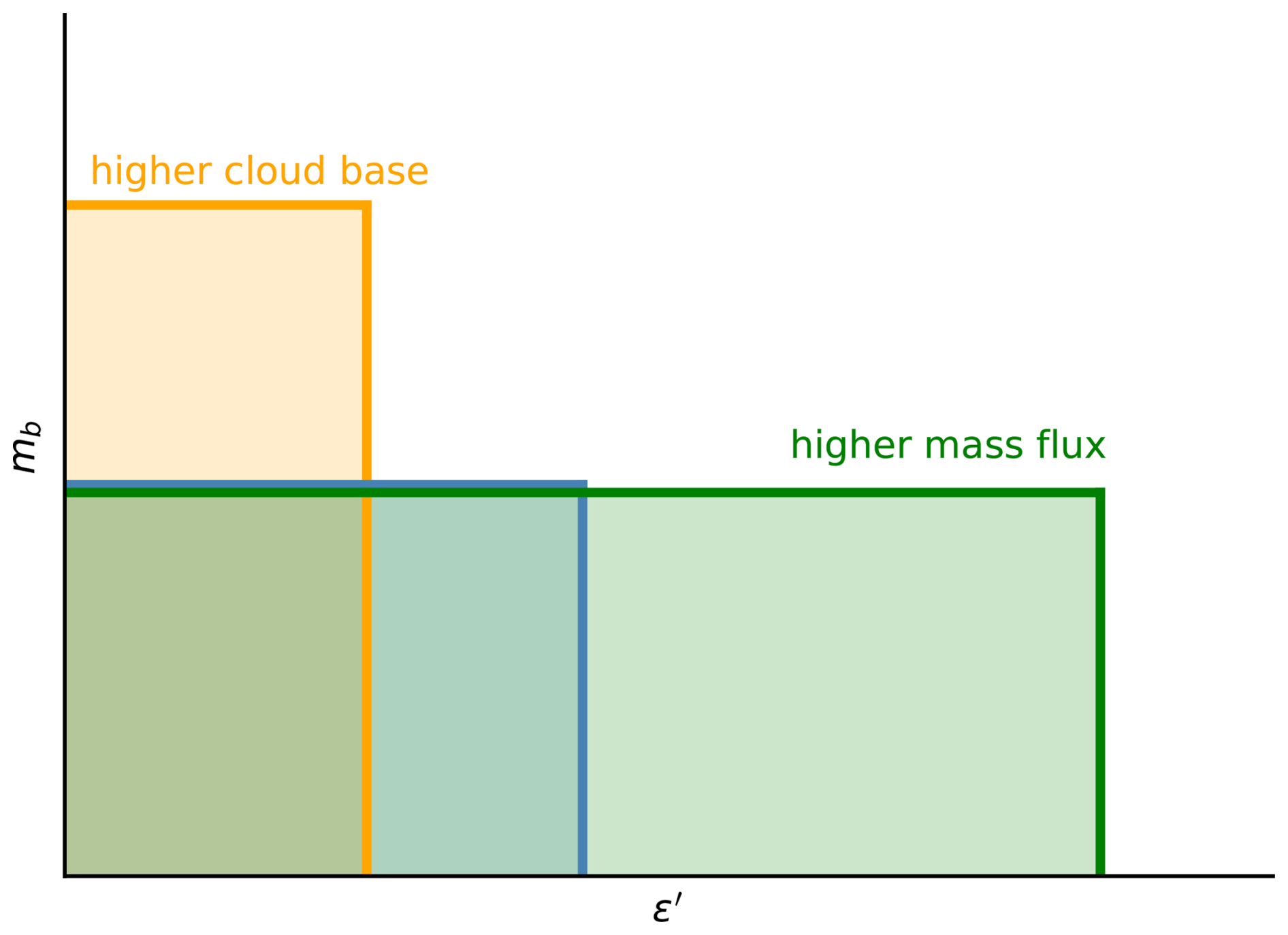
Figure 1 Distributions of cloud-base mass flux m_b(ϵ^′) as a function of the entrainment rate ϵ^′. The total cloud-base flux M_b is given by the shaded areas. Considering the blue shading as the control case, for a given total mass flux, a higher cloud base reduces the range of entrainment rates for which plumes are buoyant (orange). For a given cloud-base height, a higher mass flux is produced by increasing the range of entrainment rates for which plumes are buoyant (green).

With uniform m_b(ϵ^′), the integral in Eq. (7) may be evaluated analytically:

$$\begin{array}{}\text{(8)}& M\left(z\right)={\displaystyle \frac{M_{\mathrm{0}}}{{\mathit{ϵ}}_{\mathrm{0}}}}\left({\displaystyle \frac{e^{\mathit{ϵ}\left(z\right)(z-z_{\mathrm{b}})}-\mathrm{1}}{z-z_{\mathrm{b}}}}\right).\end{array}$$

This equation may be rearranged for the entrainment rate ϵ(z),

$$\begin{array}{}\text{(9)}& \mathit{ϵ}\left(z\right)={\displaystyle \frac{\ln \left(\frac{M_{\mathrm{b}}}{M_{\mathrm{0}}}\mathit{\eta }\left(z\right)\frac{E}{z_{\mathrm{b}}}(z-z_{\mathrm{b}})+\mathrm{1}\right)}{z-z_{\mathrm{b}}}},\end{array}$$

where we have expressed the mass flux M(z)=M_bη(z) as a product of the cloud-base mass flux and a vertical structure function η(z). Finally, we relate ϵ(z) to the areal-mean precipitation rate. To do so, we assume that the precipitation efficiency is invariant, so that the precipitation rate may be taken to be proportional to the mass flux of humidity through cloud base: $P\propto M_{\mathrm{b}}{q}^{\ast }\left(z_{\mathrm{b}}\right)$, where q^∗(z_b) is the saturation specific humidity at cloud base. This allows us to write

$$\begin{array}{}\text{(10)}& \mathit{ϵ}\left(z\right)={\displaystyle \frac{\ln \left(\frac{P}{P_{\mathrm{0}}}\mathit{\eta }\left(z\right)\frac{E}{z_{\mathrm{b}}}(z-z_{\mathrm{b}})+\mathrm{1}\right)}{z-z_{\mathrm{b}}}}\end{array}$$

where P₀≈0.125 mm h⁻¹ is the precipitation rate in radiative–convective equilibrium (e.g., Tompkins and Craig, 1998). While the precipitation efficiency is likely to be sensitive to properties such as the environmental relative humidity, we assume it is constant here for simplicity and postpone incorporating a varying precipitation efficiency to future work.

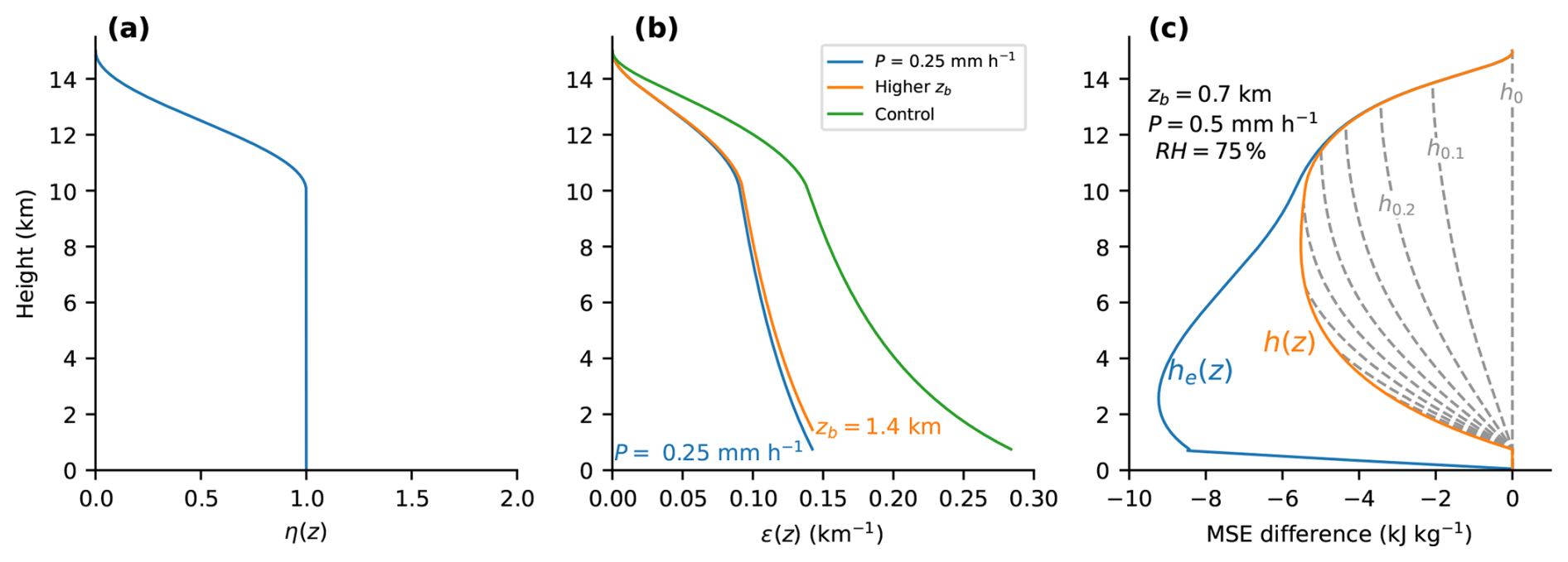
Figure 2 Vertical profiles of the SPM. (a) Mass flux vertical structure function η(z), as defined by Eq. (11). (b) The entrainment rate ϵ(z) of the plume that detrains at each height. Control case (green line) is for E=0.15, z_b=0.7 km, and P=0.5 mm h⁻¹. (c) Solution of the SPM for the control case and RH=75 %. Shown are the moist static energy of the environment h_e, of the plume that detrains at each height h(z), and of plumes h_f with entrainment rates equal to a fraction $f=(\mathrm{0},\mathrm{0.1},\mathrm{0.2},\mathrm{\dots },\mathrm{0.9})$ of the maximum entrainment rate at cloud base ϵ(z_b). All values are plotted as differences from the most static energy of the plume at cloud base h(z_b).

Equation (10) gives ϵ(z) as a function of the precipitation rate, the cloud-base height and the structure function η(z). For the present discussion, we adopt a simple profile of η(z) as shown in Fig. 2a; it remains constant up to 10 km and then decreases smoothly to zero at 15 km following

$$\begin{array}{}\text{(11)}& \mathit{\eta }\left(z\right)=\left\{\begin{array}{ll}\mathrm{1}& z\le \mathrm{10}\mathrm{km},\\ \frac{\mathrm{1}}{\mathrm{2}}+\frac{\mathrm{1}}{\mathrm{2}}\cos \left(\frac{\mathit{\pi }(z-\mathrm{10}\mathrm{km})}{\mathrm{5}\mathrm{km}}\right)& \mathrm{10}\mathrm{km}<z\le \mathrm{15}\mathrm{km},\\ \mathrm{0}& z>\mathrm{15}\mathrm{km}.\end{array}\right.\end{array}$$

Based on this mass-flux profile, Fig. 2b shows profiles of ϵ(z) for the control case of E=0.15, z_b=0.7 km and P=0.5 mm h⁻¹, and for cases with a larger cloud-base height (z_b=1.4 km) and smaller precipitation rate (P=0.25 mm h⁻¹). As expected, the entrainment rate decreases with cloud-base height and increases with the precipitation rate. In each case, ϵ(z) decreases with height, partially to counteract the growth of plumes through entrainment, and additionally, at heights above 10 km, due to the decrease in total mass flux following η(z).

While the form of η(z) has important effects on the entrainment and moist static energy at upper levels, the relationships between convection and the large-scale thermodynamic profiles described in the next section are insensitive to, for example, the inclusion of a mid-tropospheric maximum in η(z). We note, however, that a valid solution of the model only exists if ϵ(z) is monotonically decreasing with height, and this puts some limits on the mass-flux profile.

2.2 Solution procedure

Armed with the profile of ϵ(z) and a given value of the tropospheric relative humidity RH, we may solve the SPM for the thermodynamic profiles of the plume spectrum and the environment following Zhou and Xie (2019). We initialise the plume spectrum and environment with a surface temperature of 300 K and a surface humidity calculated iteratively such that z_b is at the lifted condensation level (LCL). An exact formula for the LCL was derived by Romps (2017), but it depends implicitly on the surface humidity, necessitating an iterative solution. In the sub-cloud layer, we assume the plume conserves its specific humidity, while the environmental relative humidity is linearly interpolated from the surface value to that of the free-troposphere. Both plume and environment are assumed to have constant virtual potential temperature below z_b.

Above cloud base, we solve Eq. (3) for the moist static energy profile h(z) and the moist static energy of the environment h_e(z) using a simple first-order Euler method. We do not consider the effect of liquid or solid condensate, but, unlike in the approximate equation Eq. (5), we consider the effect of moisture on the density of air. At each step, the moist static energy of the detraining plume h(z) is inverted assuming saturation to find the plume virtual temperature, which is equal to the virtual temperature of the environment. Using the free tropospheric relative humidity RH, the environmental temperature, specific humidity, and moist static energy h_e may be calculated, allowing the integration to continue upwards until the level at which M(z)=0 at z=15 km. An example solution is shown in Fig. 2c.

Once the environmental properties have been found, the moist static energy of individual plumes may be calculated via Eq. (2). Examples are shown in Fig. 2c for entrainment rates equal to $(\mathrm{0},\mathrm{0.1},\mathrm{\dots },\mathrm{0.9}){\mathit{ϵ}}_{\mathrm{b}}$, where ϵ_b is the maximum entrainment rate of buoyant plumes at cloud base. Each of these plumes therefore represents a decile of the mass-flux distribution at cloud base.

For each plume, we may calculate the integrated buoyancy

$$\begin{array}{}\text{(12)}& B_{\mathrm{int}}=\underset{z_{\mathrm{b}}}{\overset{z_{\mathrm{t}}}{\int }}g{\displaystyle \frac{T_{\mathrm{vp}}-T_{\mathrm{ve}}}{T_{\mathrm{ve}}}}\mathrm{d}z,\end{array}$$

where T_vp and T_ve are the virtual temperatures of the plume and environment, respectively, and z_t is the height at which the plume becomes neutrally buoyant. We consider two measures of the convective intensity. Firstly, we define CAPE as the value of B_int for a plume with zero entrainment. Secondly, we define the extreme convective updraft velocity as

$$\begin{array}{}\text{(13)}& w_{\mathrm{ext}}=\sqrt{\mathrm{2}{B}_{\mathrm{int}}\left(\mathrm{0.1}{\mathit{ϵ}}_{\mathrm{b}}\right)},\end{array}$$

that is, a simple measure of the maximum vertical velocity associated with the top decile of the updraft distribution.

2.3 The stability–humidity plane

We visualise the solutions of the SPM using the “stability–humidity plane” introduced by Palmer and Singh (2024, 2025) to quantify the effect of entrainment on the tropospheric lapse rate (Singh and O'Gorman, 2013). This phase plane plots the vertical difference of the saturation moist static energy $\mathrm{\Delta }{h}_{\mathrm{e}}^{\ast }$ on the ordinate against the mean saturation deficit $l_{\mathrm{v}\mathrm{0}}\stackrel{\mathrm{‾}}{(q_{\mathrm{e}}^{\ast }-q_{\mathrm{e}})}$ (expressed in energy units) on the abscissa, each defined between the 500 and 850 hPa levels in the lower troposphere. Since h^∗ is a function of temperature and pressure only, the difference $\mathrm{\Delta }{h}_{\mathrm{e}}^{\ast }$ is a function of the mean lapse rate of the lower troposphere and represents a measure of stability, with less negative values representing a more stable lower troposphere. The mean saturation deficit $l_{\mathrm{v}\mathrm{0}}\stackrel{\mathrm{‾}}{(q_{\mathrm{e}}^{\ast }-q_{\mathrm{e}})}$ represents a measure of humidity, with larger values corresponding to a drier atmosphere.

The variables $\mathrm{\Delta }{h}_{\mathrm{e}}^{\ast }$ and $l_{\mathrm{v}\mathrm{0}}\stackrel{\mathrm{‾}}{(q_{\mathrm{e}}^{\ast }-q_{\mathrm{e}})}$ are chosen because their ratio is closely connected to the entrainment rate ϵ(z) of the SPM. To see this, consider Eq. (5) and vertically integrate both sides between the 850 and 500 hPa levels. Neglecting the variation of ϵ(z) with height, so that λ≈0, this gives

$$\begin{array}{}\text{(14)}& \mathrm{\Delta }{h}_{\mathrm{e}}^{\ast }=-\stackrel{\mathrm{‾}}{\mathit{ϵ}}\mathrm{\Delta }z{l}_{\mathrm{v}\mathrm{0}}\stackrel{\mathrm{‾}}{(q_{\mathrm{e}}^{\ast }-q_{\mathrm{e}})},\end{array}$$

where Δz is the vertical distance between 850 and 500 hPa, and $\stackrel{\mathrm{‾}}{\mathit{ϵ}}$ represents an average entrainment rate that we refer to as the effective entrainment rate. For a fixed Δz, constant values of the effective entrainment rate are represented by diagonal lines on the stability–humidity plane (Fig. 3).

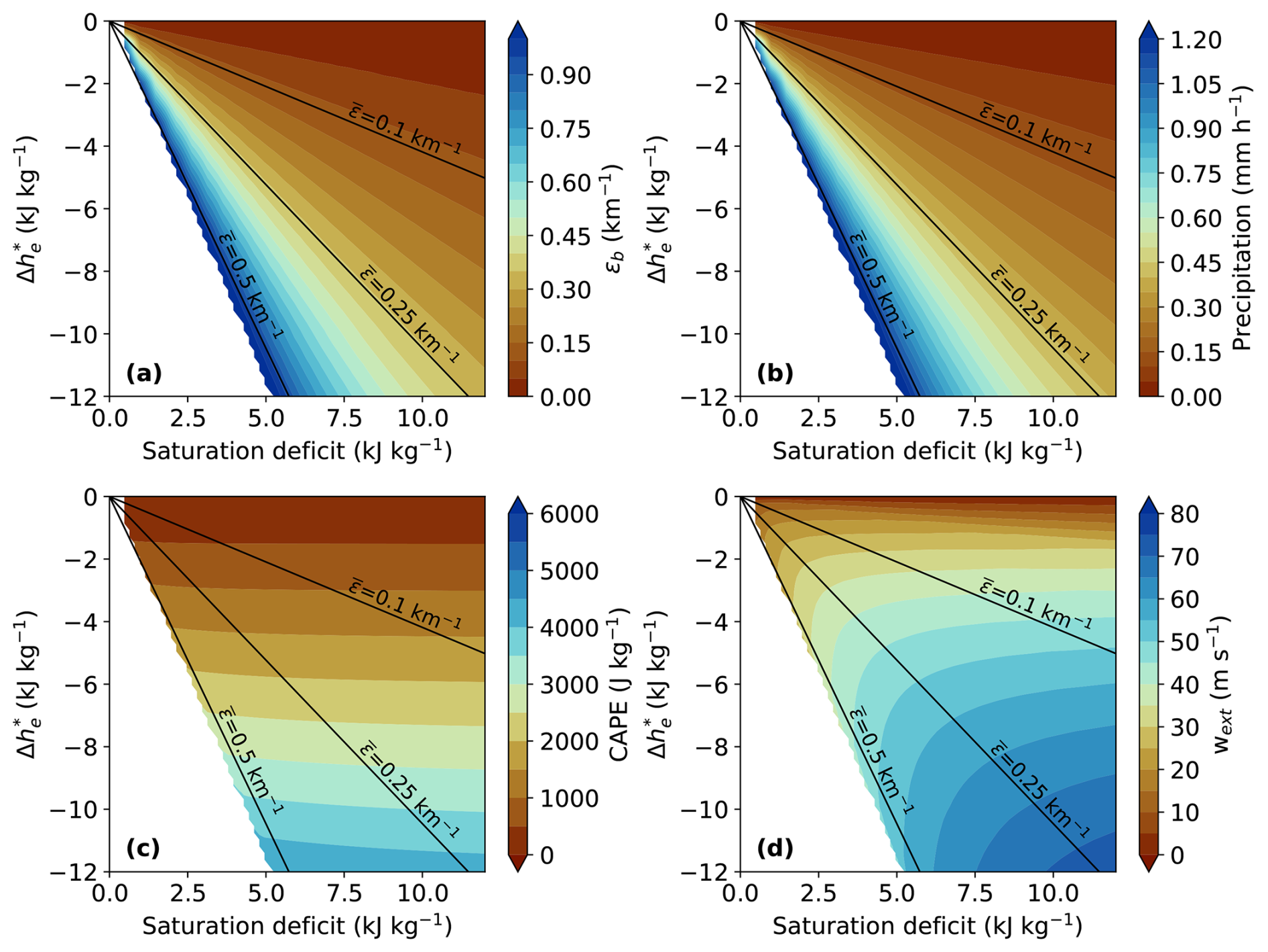
Figure 3 Solution to the SPM for z_b=1.4 km and precipitation rates between 0 and 1.25 mm h⁻¹ and tropospheric relative humidities between 2 % and 98 % in the stability–humidity plane. (a) Maximum entrainment rate at cloud base ϵ_b, (b) areal-mean precipitation rate, (c) CAPE, and (d) extreme convective updraft velocity w_ext. In each panel, effective entrainment rates $\stackrel{\mathrm{‾}}{\mathit{ϵ}}$ are calculated using Δz=4.18 km, the mean across all solutions. The white areas in each panel indicate combinations of stability and saturation deficit that are not produced by the SPM within the prescribed ranges of precipitation and relative humidity.

Palmer and Singh (2024) showed that, during precipitation, the atmosphere tends to lie in an elongated region centred on the line $\stackrel{\mathrm{‾}}{\mathit{ϵ}}=\mathrm{0.25}$ km⁻¹ and interpreted this as evidence for the effect of entrainment on the lapse rate. Here, we examine how convection varies in different regions of the stability–humidity plane according to the SPM. To do this, we calculate solutions of the SPM for z_b=1.4 km and for a range of tropospheric relative humidities RH between 2 % and 98 % and areal-mean precipitation rates P between 0 and 1.25 mm h⁻¹. For each solution, we calculate the parameters $\mathrm{\Delta }{h}_{\mathrm{e}}^{\ast }$ and $l_{\mathrm{v}\mathrm{0}}\stackrel{\mathrm{‾}}{(q_{\mathrm{e}}^{\ast }-q_{\mathrm{e}})}$, providing its location on the stability–humidity plane. The solutions spread out in two dimensions to fill most of the plane, except for the lower left corner. Interpolating the solutions to a regular grid allows us to contour various convection-related quantities in the stability–humidity plane in Fig. 3.

Variations in the maximum entrainment rate at cloud base ϵ_b closely follow those of the effective entrainment rate $\stackrel{\mathrm{‾}}{\mathit{ϵ}}$, albeit with slightly higher magnitudes (Fig. 3a). This supports our use of the stability–humidity plane and indicates it is a useful method to constrain convective entrainment using only large-scale fields (Palmer and Singh, 2024).

According to the SPM, cloud-base entrainment is a strong function of the areal-mean precipitation rate (cf. Eq. 10), and as a result, precipitation increases with both instability and humidity, peaking along the lower left portion of the phase plane (Fig. 3b). While the strong relationship between precipitation and environmental humidity is well known (Bretherton et al., 2004), the sensitivity of precipitation to both environmental humidity and lapse rate in the SPM is consistent with recent work casting the precipitation–humidity relationship in terms of the buoyancy of an entraining plume (e.g., Ahmed and Neelin, 2018).

Figure 3c and d show the distribution of SPM-derived convective intensity measures in the stability–humidity plane. Because CAPE is calculated for an undiluted parcel, it is largely a function of instability, with little humidity dependence, increasing downwards in the stability–humidity plane. On the other hand, the extreme updraft w_ext increases primarily with instability but also exhibits a weak dependence on humidity owing to entrainment, with larger values occurring in a drier atmosphere. This dependence is weak across much of the phase space but becomes more pronounced for high entrainment rates ($\stackrel{\mathrm{‾}}{\mathit{ϵ}}>\mathrm{0.25}$ km⁻¹), where strongly entraining plumes can maintain large vertical velocities only if the entrained air is relatively moist, which limits the dilution of updraft buoyancy. The top decile of the updraft distribution is therefore largest when the atmosphere is far from saturation, in stark contrast to the largest area-mean precipitation rates, which are highest near saturation. The explanation for this is that, in a dry atmosphere, the convective mass flux tends to be smaller, and only plumes with relatively small entrainment rates remain buoyant, resulting in higher average buoyancy within clouds. Thus given percentiles of the mass-flux distribution increase in intensity as the atmosphere becomes drier, even though the maximum possible updraft, associated with an undilute plume, does not. This is consistent with the argument of Louf et al. (2019) that only larger and more intense convective cells are able to penetrate into the free troposphere when it is dry. We note, however, that the SPM does not directly consider convective inhibition, which Louf et al. (2019) found to be larger in a drier atmosphere and could also prevent weaker convective cells from developing.

Finally, we consider the effect of changing cloud-base height z_b on the SPM solutions. Plotting results in the stability–humidity plane reveals that, when the cloud-base height is varied, the SPM predicts similar dependencies between the convection and its environment, but with different absolute magnitudes of the convective variables (not shown). To visualise these differences, Fig. 4 plots the effective entrainment rate as a function of the areal-mean precipitation rate for two different values of z_b. Solutions for all values of RH are shown, but they almost collapse to a line. Given our definition of the cloud-base mass-flux distribution, we expect entrainment to decrease with z_b. Indeed, for low-to-moderate precipitation rates, the effective entrainment rate is lower when the cloud base is increased to 1.4 km, although the increase is relatively modest, and in fact reverses at very heavy precipitation rates (Fig. 4). This reversal is associated with a mismatch between the cloud-base entrainment rate ϵ_b and the effective entrainment rate measured over the region between 500 and 850 hPa because of a sharp decrease in saturation moist static energy below 850 hPa. For very high areal-average precipitation rates, entrainment may be better estimated from the variation in $h_{\mathrm{e}}^{\ast }$ nearer to cloud base.

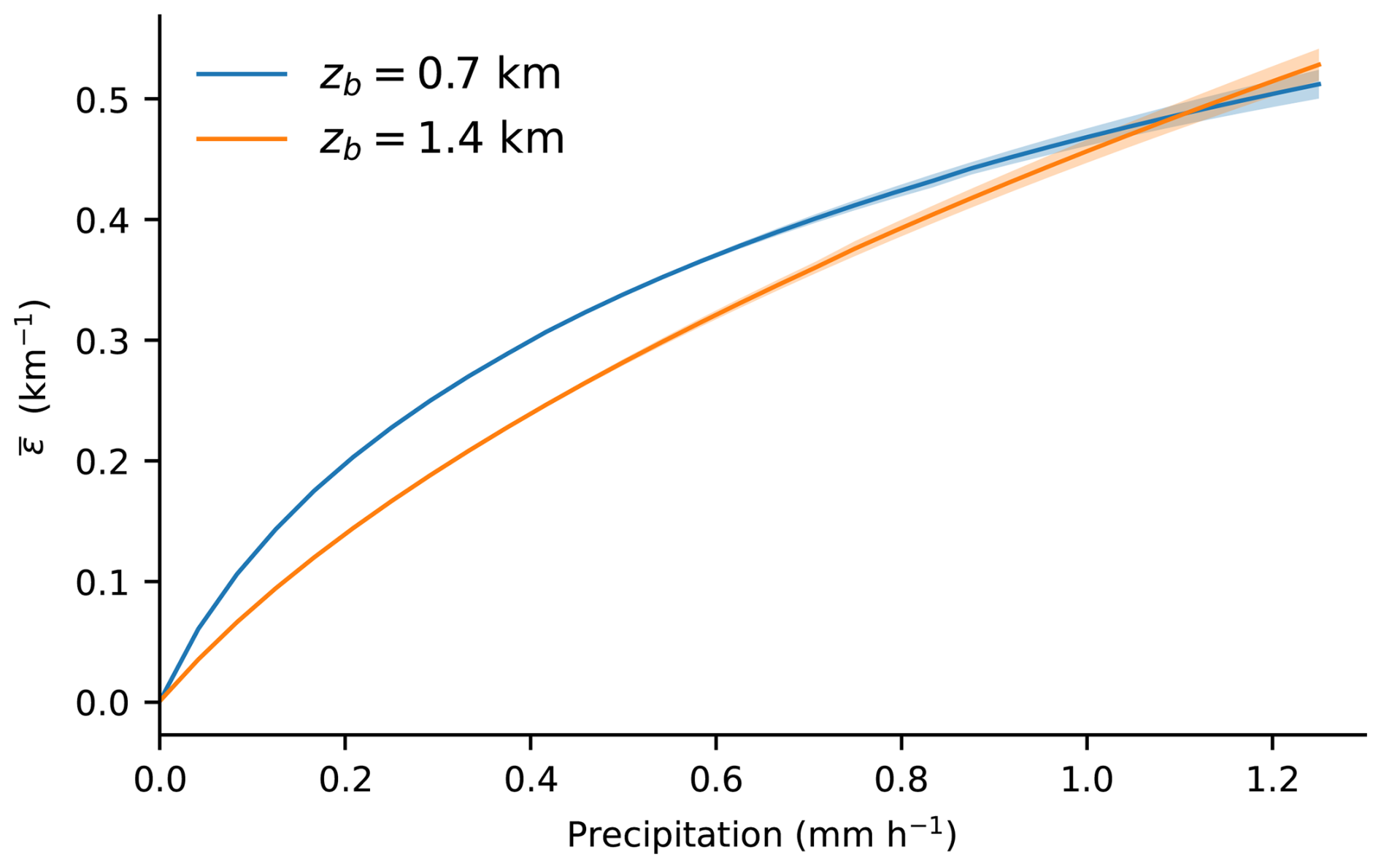
Figure 4 Effective entrainment rate $\stackrel{\mathrm{‾}}{\mathit{ϵ}}$ as a function of the areal-mean precipitation rate P for solutions of the SPM with cloud-base height z_b equal to 0.7 km (blue) and 1.4 km (orange). Solutions are plotted for relative humidities in the range 2 %–98 % (shading) with mean value given by the solid line.

In summary, the SPM solutions show large area-mean precipitation rates to be concentrated in the lower-left of the stability–humidity plane, while the strongest local convection, which we expect to be associated with the strongest local precipitation rates, is concentrated either in the lower or the lower-right portion of the phase plane, depending on whether it approaches the undilute limit. Increases in cloud base height can shift the results to a lower effective entrainment rate with the same overall dependencies. We now seek to test these predictions using radar observations and reanalysis data. A caveat to note in these comparisons is that the SPM does not predict the relative frequency in the phase plane; it does not indicate how rarely or commonly a given position in the stability–humidity plane is occupied in the tropics. We return to this point in the discussion.

3 Observational data

We now describe the observational data we use to compare the SPM to the real atmosphere. Convection and its morphology are characterised using rainfall estimates from a long-term radar archive over Darwin, Australia, while the environment is estimated using an atmospheric reanalysis over the same region.

3.1 Radar data and convective morphology

We use radar data provided by the Australian Unified Radar Archive (AURA), which is maintained by the Australian Bureau of Meteorology (Soderholm et al., 2022). We focus on the operational C-band radar located at Berrimah, Darwin (12.456° S, 130.927° E) for the 20-year period from December 2001 to 2021. We use the Level 2 rain rate and the convective–stratiform partitioning products in AURA. The rain rate fields are derived using the reflectivity fields from the lowest available scan above ground level, with reflectivity and rain rate related by an empirically derived relationship of the form Z=260.6R^1.21, where Z is the reflectivity and R is the rain rate in mm h⁻¹. This is a standard approach for obtaining instantaneous rain rate from single-polarisation radar data. The convective–stratiform classification is based on the algorithm developed by Steiner et al. (1995) and applied to gridded reflectivity at 2.5 km above radar level. The radar data have been quality controlled to remove non-meteorological echoes and artefacts. Details of data calibration and the convective–stratiform classification can be found in Bowden et al. (2024) and citations therein.

The Level 2 AURA data provide precipitation estimates at a spatial resolution of 1 km within a radius of 150 km from the radar site. The temporal resolution is 10 min before October 2018 and typically 5–6 min thereafter. Following Bowden et al. (2024), we restrict the analysis to pixels within a 100 km radius to minimise range-related artefacts. No minimum radius exclusion is applied, although manual inspection indicates that some near-radar pixels affected by the cone of silence are already masked in the radar product. Rainfall events are identified using a threshold applied to the time series of domain-mean rain rate, calculated as the total rainfall within the 100 km radius divided by the full area of that domain (i.e., including non-precipitating pixels). An event begins when the domain-mean rain rate first exceeds 0.1 mm h⁻¹ and ends when it falls below this threshold. Only events with a duration of at least 1 h are retained to exclude non-meteorological echoes. These identified rainfall events contain a total of 175 610 individual radar scenes. Only these radar scenes are used in the analysis.

For each radar scene, the domain-mean rain rate is used to characterise large-scale rainfall, with higher values indicating precipitation distributed over a larger fraction of the analysis domain. To quantify local intensity, individual pixel values are not used directly because they may be contaminated by ground clutter and random noise. Instead, we identify convective cells as connected regions of convective pixels using eight-neighbour connectivity. We then compute the cell-mean rain rate for each identified convective cell, and we define the maximum cell-mean rain rate among all convective cells within the domain as the measure of local intensity. A high maximum cell-mean rain rate indicates that intense precipitation is concentrated within a small spatial footprint. To reduce the influence of small, short-lived echoes and residual non-meteorological artifacts, only convective cells with an area greater than 5 km² are considered. As a sensitivity test, we alternatively use the 90th-percentile pixel-wise rain rate within each cell as a measure of local convective intensity. This produced results similar to those obtained using the cell-mean rain rate (not shown); therefore, we only present results based on the maximum cell-mean rain rate. To minimise edge effects, cells intersecting the 100 km radius boundary are retained in their entirety, rather than restricting the analysis to only the portion within the domain. Very large systems (e.g. long squall lines) may still be truncated at 150 km, but would still be identified as large systems.

The convective and stratiform contributions to the domain-mean precipitation are calculated using the AURA convective–stratiform partitioning product. For each radar scene, convective rainfall contribution is defined as the sum of rain rate over pixels classified as convective, divided by the sum over all precipitating pixels of the 100 km-radius analysis domain; stratiform rainfall is calculated analogously using pixels classified as stratiform.

For spatial characteristics of convection, we focus on the identified convective pixels and exclude pixels classified as stratiform. With this convective–stratiform separation, only moderate to deep convection is considered, and weakly or non-precipitating shallow clouds are excluded. Following Louf et al. (2019), we calculate the number of convective cells (N) and the area (A) of each cell for each radar scene. This gives the convective area fraction (CAF) of each radar scene as:

$$\begin{array}{}\text{(15)}& \mathrm{CAF}={\displaystyle \frac{\mathrm{1}}{D}}\sum _{i=\mathrm{1}}^N{A}_i,\end{array}$$

where D is the total area of the radar domain, including non-raining pixels (∼ 31 400 km²) and A_i is the area of each individual convective cell. The morphology of convective cells is represented by the number of cells (N) and the mean cell area:

$$\begin{array}{}\text{(16)}& \stackrel{\mathrm{‾}}{A}={\displaystyle \frac{\mathrm{1}}{N}}\sum _{i=\mathrm{1}}^N{A}_i.\end{array}$$

3.2 Environmental conditions

Large-scale environmental conditions are obtained from the fifth generation of the European Centre for Medium-Range Weather Forecasts (ECMWF) atmospheric reanalysis (ERA5; Hersbach et al., 2020). The ERA5 data are on a 0.25° × 0.25° grid on 37 pressure levels with hourly temporal resolution. Following Louf et al. (2019), the environmental conditions are linearly interpolated to the temporal resolution of the radar data. To characterise the large-scale environment, we use ERA5 data from a 3° by 3° area centred on the radar (11–13.75° S, 129.5–132.25° E; 12 by 12 grid points).

Our primary environmental variables are the stability $\mathrm{\Delta }{h}_{\mathrm{e}}^{\ast }$ and the saturation deficit $l_{\mathrm{v}\mathrm{0}}\stackrel{\mathrm{‾}}{(q_{\mathrm{e}}^{\ast }-q_{\mathrm{e}})}$ defined in the previous section. They are calculated using ERA5 temperature and specific humidity at pressure levels between 850 and 500 hPa, and averaged over the radar domain. We also use CAPE, convective inhibition (CIN), and boundary-layer height (BLH) obtained from the ERA5 single-level dataset. CAPE is calculated as the integrated positive buoyancy of an air parcel lifted pseudo-adiabatically, including freezing and a mixed-phase range. Parcels are lifted from all model levels below the 350 hPa level, and the “most unstable parcel”, leading to the maximum CAPE, is retained (ECMWF, 2026). Note that, for computational efficiency, the calculation procedure of CAPE and CIN in ERA5 uses an approximation that neglects the effect of water vapour on density. This may lead to an underestimation of CAPE and overestimation of CIN (Davies, 2004). Nevertheless, for simplicity, we use the CAPE and CIN provided by ERA5 and discuss these limitations in Sect. 5.

CIN quantifies the energetic barrier that must be overcome for a parcel to reach its level of free convection (LFC). It is calculated as the integrated negative buoyancy below the LFC of the most unstable parcel defined above (ECMWF, 2026). This gives CIN positive values, with larger values indicating stronger inhibition. While CIN suppresses weak ascent, sufficiently strong lifting can overcome it and subsequently permit vigorous deep convection. The spatial maximum CAPE and maximum CIN within the analysis domain are used to represent the most unstable conditions and the strongest inhibition, respectively. The BLH in ERA5 is diagnosed using the bulk Richardson number, following Seidel et al. (2012). As a secondary measure of the depth of the sub-cloud layer, we calculate the LCL from ERA5 surface pressure and 2 m temperature and dewpoint temperature using the MetPy package (May et al., 2022, 2025), based on Romps (2017).

4 The observed thermodynamic-convection relationship

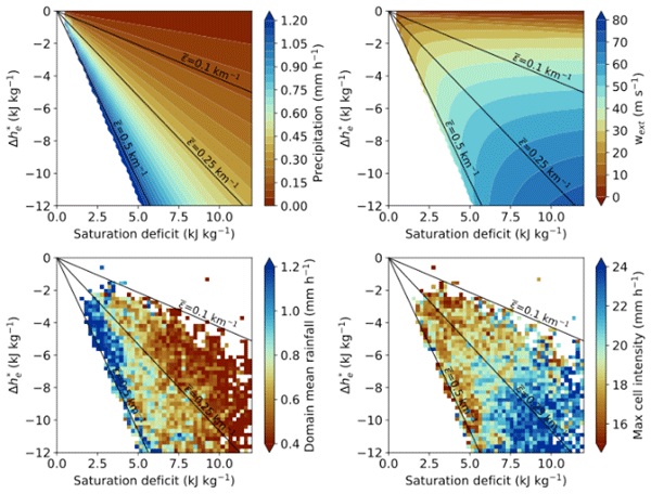
We now consider observed properties of convection in the stability–humidity plane. Radar scenes are binned by values of the stability $\mathrm{\Delta }{h}_{\mathrm{e}}^{\ast }$ and the saturation deficit taken from ERA5, both spatially averaged over the radar domain. Figure 5a shows the number of radar scenes included in each 2D histogram bin. Most of the data fall between the effective entrainment rates of 0.1 and 0.5 km⁻¹, and there is a clear relation; a drier atmosphere tends to be more unstable. Given that all 175 610 radar scenes are drawn from identified rainfall events, this result is consistent with that of Palmer and Singh (2024). They analysed the large-scale environment from reanalysis and radiosonde observations associated with precipitation exceeding 5 mm d⁻¹, defined from reanalysis precipitation and station precipitation, respectively. They used the stability–humidity plane to describe precipitating regions and showed a pattern similar to Fig. 5a across tropical oceans. While the SPM does not predict the relative frequency with which the atmosphere occupies different locations in the stability–humidity plane, this correlation provides evidence for a role for entrainment in setting the local lapse rate over Darwin (Palmer and Singh, 2024).

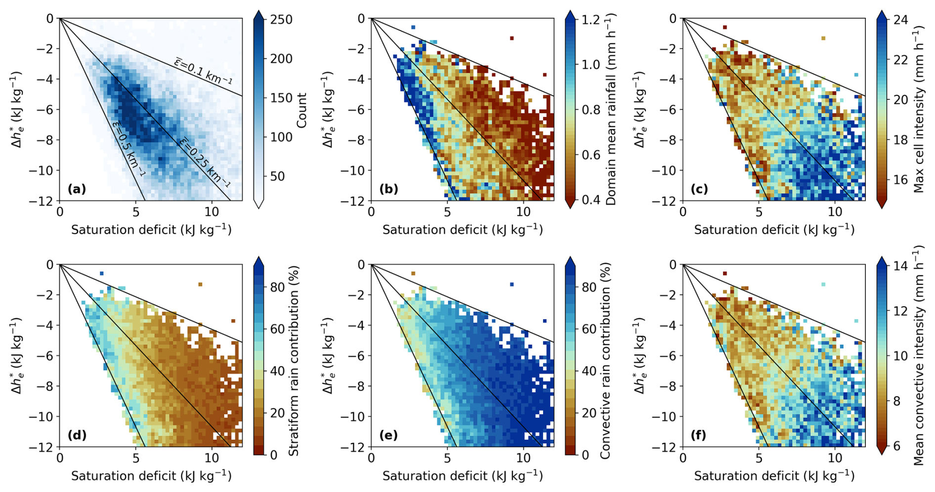
Figure 5 Observed properties of convection in the stability–humidity plane. (a) Frequency distribution of radar scenes binned by stability $\mathrm{\Delta }{h}_{\mathrm{e}}^{\ast }$ and saturation deficit $l_{\mathrm{v}\mathrm{0}}\stackrel{\mathrm{‾}}{(q_{\mathrm{e}}^{\ast }-q_{\mathrm{e}})}$ calculated from ERA5. (b–f) Average properties of radar scenes binned by $\mathrm{\Delta }{h}_{\mathrm{e}}^{\ast }$ and $l_{\mathrm{v}\mathrm{0}}\stackrel{\mathrm{‾}}{(q_{\mathrm{e}}^{\ast }-q_{\mathrm{e}})}$ showing (b) domain-mean rainfall, (c) maximum convective cell intensity, (d) stratiform rain contribution, (e) convective rain contribution, and (f) mean convective rain intensity. Only bins with at least 30 data points are shown. Solid black lines give effective entrainment rates as labelled in panel (a), calculated using Eq. (14) with Δz=4.27 km, corresponding to the mean difference in height between the 850 and 500 hPa levels for the Darwin radar region in ERA5 between 2001 and 2021.

4.1 Areal-mean precipitation and local intensity

To compare the predictions of the SPM to observations, the radar domain mean rainfall and the maximum convective cell intensity of each radar scene are plotted in the stability–humidity plane in Fig. 5b and c, respectively. The value of each 2D histogram bin is the mean of all scenes falling within that bin. Only bins with more than 30 scenes are included in the analysis. Consistent with the SPM predictions (Fig. 3), the areal-mean precipitation increases with both humidity and instability, peaking in the lower-left region of the phase plane. That is, the mean rain rate over the radar domain increases with the effective entrainment rate $\stackrel{\mathrm{‾}}{\mathit{ϵ}}$.

It may seem counter-intuitive that heavier large-scale precipitation is associated with higher effective entrainment rates $\stackrel{\mathrm{‾}}{\mathit{ϵ}}$. But in the framework of the SPM, $\stackrel{\mathrm{‾}}{\mathit{ϵ}}$ does not represent the dilution experienced by individual clouds. Rather, it characterises how the large-scale environment adjusts to restore buoyancy neutrality under convective activity. When precipitation is widespread, a large number of plumes must be buoyant, requiring an unstable and moist environment. In this context, a higher $\stackrel{\mathrm{‾}}{\mathit{ϵ}}$ is consistent with more extensive convective activity.

In the radar observations, the rainfall may be separated into stratiform and convective types; stratiform rainfall contributes an increasing fraction of the domain-mean rainfall as the atmosphere becomes moister, and as $\stackrel{\mathrm{‾}}{\mathit{ϵ}}$ becomes larger (Fig. 5d–e). This agrees with previous studies demonstrating that the strong observed increase in precipitation with moisture is largely associated with enhanced stratiform rainfall through expansion of the rain area, rather than intensified convection (Ahmed and Schumacher, 2015). The SPM, however, does not have an explicit representation of stratiform rainfall, and it can only produce large area-averaged precipitation through widespread convection.

Unlike the domain-mean rain rate, the maximum cell-mean convective rainfall intensity is largest in a drier and more unstable atmosphere, peaking in the bottom right of the stability–humidity plane (Fig. 5c), consistent with the behaviour of the extreme updraft velocity w_ext in the SPM (Fig. 3d). This is in agreement with Raymond et al. (2024), who found that the intense and localised “showers” develop in drier environments with larger instability. As the cell intensity depends on both total rainfall within a convective cell and the cell area, we tested the sensitivity of this relationship to the definition of intensity. The pattern shown in Fig. 5c remains evident when intensity is represented by the 99th percentile of pixel-wise rain rate calculated from rainy pixels only (not shown), indicating that the relationship is not primarily controlled by the area of the most intense convective cell. Additionally, this relationship is not limited to the most intense convective cells: when intensity is instead defined as the mean convective rain intensity across all cells, calculated as total convective rainfall divided by total convective area, the same pattern persists (Fig. 5f).

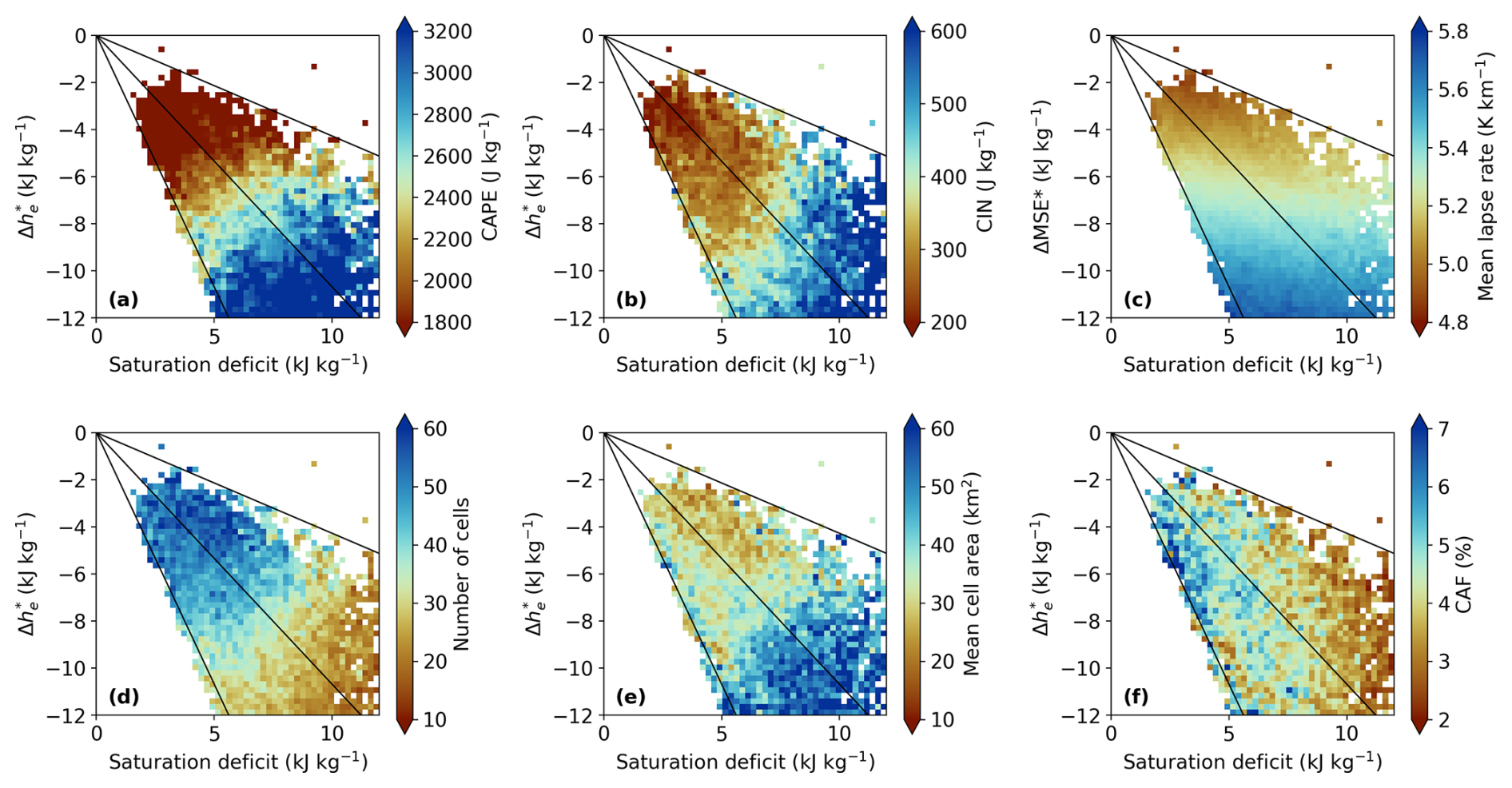
Figure 6 Same as Fig. 5, but for (a) CAPE, (b) CIN, (c) 850–500 hPa mean temperature lapse rate, (d) number of cells, (e) mean cell area, and (f) CAF. For all panels, only bins with more than 30 data points are plotted.

The higher convective intensity also coincides with the largest values of CAPE and CIN when binned in the stability–humidity plane (Fig. 6a–b), and shows little systematic relationship with $\stackrel{\mathrm{‾}}{\mathit{ϵ}}$. However, unlike in the SPM, reanalysis CAPE is not simply a function of instability $\mathrm{\Delta }{h}_{\mathrm{e}}^{\ast }$, but also increases with the saturation deficit. In the observational analysis, CAPE and convective intensity are well aligned across a number of different intensity measures, but this is not true for the strongest updrafts w_ext in the SPM. This difference may be because CAPE integrates parcel buoyancy over the depth between the LFC and the LNB, whereas our stability measure characterises only the 850–500 hPa layer. The 850–500 hPa lapse rate (Fig. 6c) does not exhibit the same pattern as CAPE (Fig. 6a), indicating that lower-tropospheric stability alone does not determine CAPE in ERA5. While the idealised SPM links CAPE solely to stability, CAPE is also influenced by the properties of the source parcel and the thermodynamic structure outside the 850–500 hPa layer. Although reanalysis-derived CAPE is known to exhibit biases relative to sounding-derived estimates, ERA5 has been shown to be one of the most reliable reanalyses for convective parameters (Taszarek et al., 2021b). A detailed interpretation of this behaviour of CAPE in the stability–humidity plane is left for future work.

In summary, the observational analysis confirms important aspects of the behaviour of the SPM. In both cases, the areal-mean rain rate increases with the effective entrainment rate, while the intensity of convection peaks when the atmosphere is drier and more unstable.

4.2 Factors hypothesised to affect convective entrainment

The correspondence between the SPM and observational analysis above suggests that the effective entrainment rate $\stackrel{\mathrm{‾}}{\mathit{ϵ}}$, diagnosed purely from large-scale fields, provides information about the level of mixing between the convective ensemble and its environment. We therefore use the stability–humidity plane to investigate factors that influence $\stackrel{\mathrm{‾}}{\mathit{ϵ}}$ and, by extension, convective mixing.

Previous studies have suggested that larger convective cells may be associated with lower entrainment because of their lower surface-area to volume ratio (e.g., Takahashi et al., 2021, 2023; Peters et al., 2026). However, the observed convective cell morphology does not support a strong influence of cell size on $\stackrel{\mathrm{‾}}{\mathit{ϵ}}$. Instead, as found by Louf et al. (2019), drier and more unstable environments are associated with a smaller number of convective cells (Fig. 6d) and a larger mean convective cell area (Fig. 6e). The largest cells occur under similar environments to the most intense convection, with a weak dependence on $\stackrel{\mathrm{‾}}{\mathit{ϵ}}$. Restricting the environmental conditions to raining pixels or considering environmental conditions 3 h prior to each radar scene does not substantially change this pattern (not shown).

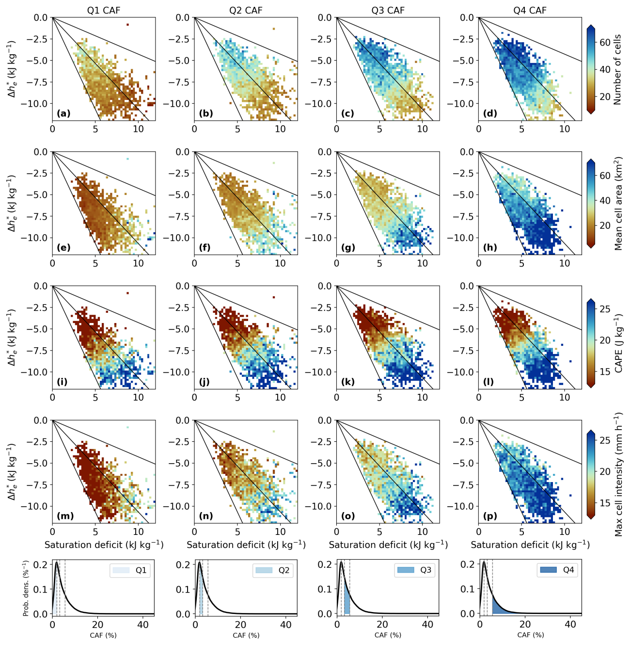
Figure 7 (a–p) Same as Fig. 5, but stratified by CAF quartiles, with each column showing a different quartile (Q1–Q4) from left to right. (a–d) Number of convective cells, (e–h) mean cell area, (i–l) CAPE, and (m–p) maximum cell intensity. In each panel of (a)–(p), only 2D histogram bins containing more than 20 radar scenes are displayed. The bottom row shows the probability density distribution of CAF and the thresholds for each CAF quartile.

A possible confounding variable in the above analysis is that of the convective area fraction (CAF). This increases strongly with the areal-mean precipitation and is therefore highest for large values of $\stackrel{\mathrm{‾}}{\mathit{ϵ}}$ (Fig. 6f). But a large CAF may also favour larger cells (Blackberg and Singh, 2026), thereby obscuring the effect of cell size on entrainment. To address this, we compare scenes with similar overall convective extent by partitioning radar scenes into four groups according to CAF quartiles. Characteristics of each quartile in the stability–humidity phase plane are shown in Fig. 7, where Q1 denotes the lowest quartile of CAF. Because partitioning the data into quartiles reduces the sample size within each group, we lower the minimum number of radar scenes required per 2D histogram bin from 30 to 20.

For a given CAF quartile, the relationships identified in Fig. 6 persist: drier and more unstable environments are associated with fewer but larger convective cells, and the relationship to $\stackrel{\mathrm{‾}}{\mathit{ϵ}}$ is weak (Fig. 7a–h). Because CAF is constrained within each quartile, this shift toward larger cells reflects increased spatial clustering rather than greater total convective coverage, indicating enhanced convective organisation. Previous studies have found contrasting effects of convective organisation on entrainment, with overall dilution tending to decrease because of the moist near-cloud environment, but an increase in mixing through increases in turbulent kinetic energy (Feng et al., 2015; Hannah, 2017; Becker et al., 2018).

Note that the above relationships of maximum cell intensity to the mean area of cells are specific to convective cells. When all raining areas are included (stratiform and convective), the mean rain cell area follows areal-mean precipitation more closely (not shown), because high areal-mean rainfall often reflects an expansion of raining area associated with stratiform precipitation (Ahmed and Schumacher, 2015).

As for the overall statistics, when stratified by CAF, CAPE and maximum cell intensity exhibit patterns similar to those of mean convective cell area (Fig. 7i–p). Higher CAPE in drier and more unstable environments coincides with stronger maximum cell intensity. This pattern is weaker in the lowest CAF quartile, for which maximum cell intensity and mean cell area depend more strongly on humidity than on stability. At low CAF, the limited convective coverage favours smaller cells, which are expected to experience greater entrainment and therefore be more sensitive to environmental humidity. Nevertheless, these results give a consistent picture of the thermodynamic conditions that favour more spatially organised and locally intense convection. Such storms form in environments in which stronger instability supports deeper, more coherent updrafts, while reduced background humidity limits the number of simultaneously active cells.

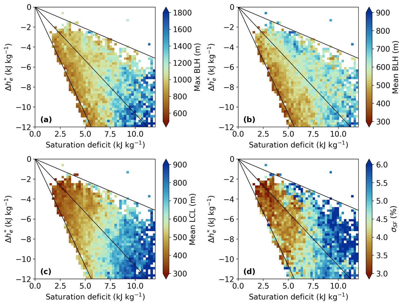
Figure 8 Same as Fig. 5, but for (a) domain maximum BLH, (b) domain mean BLH, (c) domain mean LCL, and (d) spatial standard deviation of saturation fraction (σ_SF). For all panels, only bins with more than 30 data points are plotted.

Another hypothesis is that the depth of the boundary layer may influence convective entrainment through its effect on the size of convective updrafts (Zipser and LeMone, 1980; May and Ballinger, 2007; Yang, 2018; Peters et al., 2020a; Mulholland et al., 2021; Takahashi et al., 2021, 2023; Powell, 2024). Indeed, this hypothesis informed our parameterisation of the entrainment distribution in the SPM. While our preceding results suggest that size, at least when it comes to convective rain cells, is not a strong predictor of entrainment, we nevertheless examine the behaviour of the boundary-layer height (BLH) and the LCL, as diagnosed in ERA5, binned in the stability–humidity plane. We present both the spatial maximum BLH (Fig. 8a) and the spatially averaged BLH (Fig. 8b) within the radar domain, where the maximum captures local variations, while the mean reflects the bulk boundary layer state. Only the spatially averaged LCL is shown (Fig. 8c) as the maximum LCL exhibits a similar pattern (not shown).

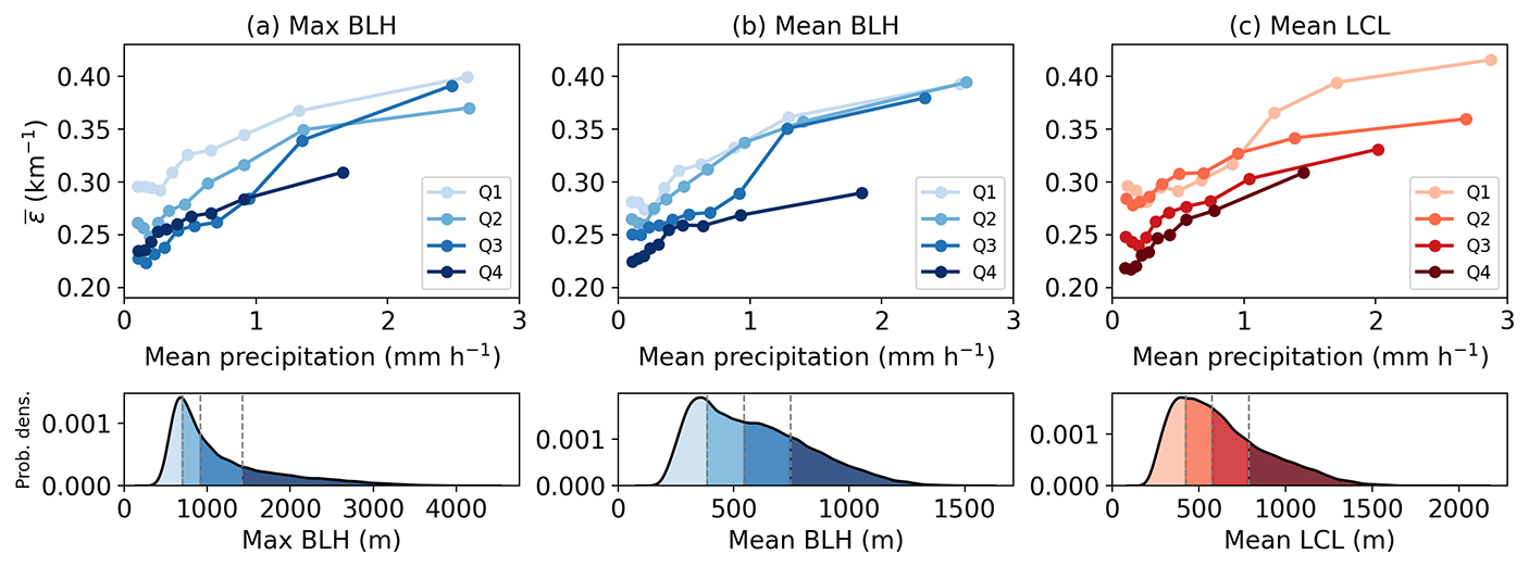
Figure 9 Effective entrainment rate $\stackrel{\mathrm{‾}}{\mathit{ϵ}}$ calculated based on the mean stability and saturation deficit from ERA5 in bins of different domain-mean precipitation from the radar. Lines show quartiles (Q1–Q4) of (a) spatial maximum BLH, (b) spatial mean BLH, and (c) mean LCL, where Q1 is the lowest quartile. The bottom row shows the probability density function of each variable in the panel above, with shading and dashed lines marking the quartile ranges and thresholds.

The results show that the mean BLH increases with both saturation deficit and stability, with contours that roughly follow those of $\stackrel{\mathrm{‾}}{\mathit{ϵ}}$. This is consistent with the argument that a deeper boundary layer reduces convective entrainment. The LCL and the maximum BLH have slightly different dependencies, with a stronger dependence on saturation deficit and weaker dependence on stability. Nevertheless, when plotted as a function of the areal-mean precipitation rate, $\stackrel{\mathrm{‾}}{\mathit{ϵ}}$ generally decreases with all measures of boundary layer depth: mean and maximum BLH and LCL (Fig. 9). Comparing Fig. 9 with Fig. 4, we see that the effective entrainment diagnosed from ERA5 has a similar dependence on entrainment to the SPM. This supports our use of the cloud-base height as a key parameter within the model's entrainment distribution.

In addition to a lower effective entrainment rate, higher values of the LCL and maximum BLH correspond to greater maximum cell intensity in the radar observations (cf. Figs. 5c and 8a, c). This is consistent with previous theoretical (Peters et al., 2026) and observational studies (Murillo et al., 2026) relating boundary layer depth to the dilution experienced by convective updrafts. For the SPM, however, a fixed CAPE has a similar value of w_ext even when the cloud-base height is reduced from z_b=1400 m to z_b=700 m (not shown). This is because the SPM considers the effect of entrainment on the environment as well as the convective ensemble, and w_ext therefore increases with a wider entrainment distribution rather than a lower mean value of entrainment. However, this result is likely sensitive to our assumption of a uniform distribution of mass flux with entrainment; further work is needed to investigate different mass flux distributions based on cloud-resolving simulations.

Finally, we consider the possible role played by spatial variability in humidity in the diagnosis of $\stackrel{\mathrm{‾}}{\mathit{ϵ}}$. The SPM assumes that the environment for each plume within the plume spectrum is the same and equal to that of the domain mean. However, small-scale humidity variability may result in a near-cloud environment substantially different to that of the mean, thereby affecting dilution produced by entrainment mixing. To test this hypothesis, we calculated the spatial standard deviation of the saturation fraction (σ_SF), using ERA5 data. Here the saturation fraction is defined as the ratio of the column-integrated water vapour divided by the same quantity assuming saturation, with the vertical integrals taken from 1000 to 100 hPa following Angulo-Umana and Kim (2023). Note that we are limited by the 0.25° resolution of the ERA5 data to consider only relatively large-scale humidity variability. Figure 8d shows that σ_SF increases with the mean saturation deficit, and is highest in environments in which the most intense convection occurs. This supports the notion that intense convection develops within moist, localised regions embedded in a drier large-scale environment (e.g., Powell, 2024). The enhanced moisture variability may also partly reflect the effects of convection itself as represented in ERA5, for example through data assimilation, rather than a pre-existing environmental control. Although we do not infer causality from this relationship, this finding points to the possible importance of small-scale variability in the environment, unaccounted for in the SPM when characterising convective mixing.

In summary, the results of this subsection provide support for a role of the depth of the boundary layer in setting the bulk entraining properties of convection. On the other hand, we found that the average size of convective rain cells was not related to the effective entrainment rate, suggesting either that the size of updrafts relevant for their mixing properties is not well captured by measures of their rainfall area, or that boundary-layer depth is related to the effective entrainment rate for reasons other than its effect on updraft size. We also noted that small-scale variability in the convective environment may cause variations in mixing that are not captured in the effective entrainment rate. Nevertheless, the overall agreement between the SPM and the observational analysis is promising, and suggests the stability–humidity phase plane is a useful tool for examining the mixing and other properties of convection, particularly for understanding and evaluating storm-resolving models.

5 Conclusions

This paper addresses the question of how heavy rainfall at different spatial scales is related to the large-scale thermodynamic environment. We developed a simple conceptual model for these relationships in which convection is represented by a spectrum of entraining plumes with different entrainment rates under the assumption that each plume detrains at its LNB. According to the spectral plume model, areal-mean rainfall and local convective intensity represent distinct modes of heavy precipitation, each associated with different large-scale thermodynamic environments. Large areal-averaged rain rates are produced by a large number of buoyant plumes, requiring a moist free-troposphere, while localised high-intensity convection requires an unstable lapse rate and is associated with only low-entrainment plumes that are more prevalent in a drier atmosphere. These predictions were tested using 20 years of radar observations and ERA5 reanalysis for Darwin, Australia. Consistent with the SPM, high domain-mean rainfall was found to be associated with more humid environments and higher effective entrainment rates, while high convective precipitation intensity occurred preferentially in drier and more unstable environments characterised by high CAPE.

The similarity of the SPM and the observational analysis motivated an examination of the properties of the convective ensemble in the stability–humidity plane (Palmer and Singh, 2024). This allows for the diagnosis of the effective entrainment rate $\stackrel{\mathrm{‾}}{\mathit{ϵ}}$, which in the SPM framework provides a bulk measure of mixing between convection and its environment. This analysis revealed that entrainment tends to be lower when the boundary layer is deeper, as has previously been hypothesised (Williams and Stanfill, 2002), but the size of convective cells was found to have little relationship to $\stackrel{\mathrm{‾}}{\mathit{ϵ}}$. Instead, a smaller number of larger, more organised cells were found to occur in similar environments to those of the most intense localised convection: a relatively dry free troposphere and large values of CAPE and CIN (Louf et al., 2019).

The reasons for the lack of dependence of the effective entrainment rate on the size of convective cells are unclear, but may be speculated upon. First, the largest cells occur in environments with large CIN, but CIN is not considered in the SPM. These cases may therefore deviate from the SPM assumption that the plume spectrum adjusts toward buoyancy neutrality with the large-scale environment. This may also account for the additional dependence of CAPE on tropospheric humidity, which, according to the SPM, is only dependent on tropospheric stability. It may also be the case that other factors have a larger effect on entrainment than the reduced surface area to volume ratio of larger convective cells. Becker et al. (2018) found higher entrainment rates in idealised simulations of aggregated convection compared to disaggregated convection due to an increase in turbulence near clouds, despite the updrafts being larger in the aggregated case. Finally, we note that under drier conditions, the lower tropospheric humidity is also more spatially variable. This variability could result in individual clouds experiencing less or more dilution than would be expected from the SPM (Hannah, 2017). This could explain the prevalence of larger convective cells under drier conditions, in which spatially organised convection increases the local humidity to protect convective cores from dry-air dilution, as found for self-aggregated convection by Becker et al. (2018).

Despite the complexity of interpretation highlighted above, the stability–humidity phase space provides a useful framework for separating distinct environmental regimes. Notably, if the observational analysis is conducted using CAPE alone, high domain-mean rainfall and high local intensity exhibit similar CAPE values (not shown), consistent with previous results for this region (May and Ballinger, 2007; Louf et al., 2019). Future work to apply the same methods to convection-permitting simulations is desirable, both to determine the relationship between the effective entrainment rate and the actual mixing produced by convective clouds, and to evaluate the behaviour of such models compared to observations.

Several limitations should be noted. Due to radar uncertainties, local intensity is defined using cell-mean rain rates rather than pixel-scale maxima, which may underestimate extreme point-wise intensities. In addition, CAPE and CIN are directly obtained from ERA5. Their calculation neglects the negative contribution of condensate loading to parcel buoyancy and reduces the positive contribution from freezing, both of which may substantially affect CAPE and CIN in moist tropical environments (Warren, 2025). Moreover, previous work has shown that long-term CAPE trends in reanalysis may be sensitive to radiosonde availability (Taszarek et al., 2021a). Although Darwin benefits from a long radiosonde record (Pope et al., 2009), caution is warranted when interpreting absolute CAPE magnitudes. The differences between CAPE in the SPM (Fig. 3c) and in ERA5 (Fig. 6a) motivate further investigation in which CAPE is recalculated from ERA5 model-level fields with the virtual temperature correction included. Such a calculation would also provide improved sampling of boundary-layer conditions relative to standard pressure-level fields (Taszarek et al., 2021b). Future work could also consider adiabatic (“reversible”) CAPE and CIN. Adiabatic CAPE with ice has been argued to be a more appropriate measure of conditional instability in the tropics (e.g. Williams and Renno, 1993), while adiabatic CIN has been found to provide a better representation of the inflow layer for simulated convective storms (Murdzek et al., 2021).

In this study, we have focused on the thermodynamic links between entrainment, convection, and the large-scale environment. Vertical wind shear may additionally influence convective organisation, updraft width, and fractional entrainment (e.g. Peters et al., 2019, 2020b; Jo and Lasher-Trapp, 2022; Maybee et al., 2024). However, its role is difficult to isolate over Darwin because both the magnitude and vertical structure of shear vary across monsoon regimes, together with changes in the thermodynamic environment. Robust attribution would require separating these interacting effects across different monsoon regimes. We therefore leave a systematic investigation of the role of vertical wind shear to future work.

While the observational analysis focuses on Darwin, the framework has broader implications for understanding heavy rainfall across the tropics. Climate projections robustly indicate increasing CAPE in a warmer climate (e.g., Singh and O'Gorman, 2013; Seeley and Romps, 2015; Chen et al., 2020; Muller and Takayabu, 2020). Our results suggest that changes in instability alone are insufficient to diagnose future changes in rainfall structure. By linking humidity, stability, entrainment, and convective organisation through the SPM framework, this study provides an observational basis for evaluating how models simulate the morphology of widespread and localised heavy precipitation and how they may evolve under climate change. Future work will extend this analysis using high-resolution satellite observations to assess the generality of these findings across the broader tropics.

Finally, it is important to emphasise that this study does not directly establish causal relationships between environmental conditions and convective morphology. The SPM calculates the temperature profile and mass-flux distribution consistent with a given precipitation rate and tropospheric humidity but does not answer the question of how that precipitation came about. Examining the detailed evolution of precipitation events in the stability–humidity plane may be a fruitful avenue toward addressing this question.