Linking European droughts to year-round weather regimes

European droughts have far-reaching socio-economic and ecological impacts, yet their prediction remains challenging due to the complex interplay between large-scale atmospheric circulation patterns and local thermodynamic processes. This study investigates how persistent North Atlantic weather regimes influence the occurrence and spatial distribution of seasonal meteorological droughts across Europe throughout the year. Using reanalysis datasets and a tailored regionalization based on drought synchronicity, we identify six coherent European sub-regions and relate drought events, defined by the standardized precipitation index (SPI3), to year-round weather regimes derived from 500 hPa geopotential height anomalies. Our analysis shows that while each weather regime exhibits distinctive and relatively stable precipitation patterns throughout the year, only a fraction of droughts – primarily in western Europe and during winter – can be directly attributed to anomalies in regime frequency. The findings underline the partial but regionally significant role of North Atlantic circulation patterns in shaping European drought risk, highlighting opportunities and limitations for improving drought forecasts on sub-seasonal to seasonal timescales. This study emphasizes the added value of using year-round weather regimes as a unifying framework for understanding drought drivers, overcoming the constraints of purely seasonal classifications. Improved understanding of these links could help refine climate models and support more robust early-warning systems for drought management across diverse European climates.

1 Introduction

Droughts are complex climate events (Dracup et al., 1980; Kallis, 2008) with potentially disastrous consequences for society and ecosystems. They are typically classified into four categories: meteorological, hydrological, agricultural, and economical droughts (Yevjevich, 1967; Wilhite and Glantz, 1985), depending on the physical variables they are associated with. These different types of droughts have various causes, consequences, and time scales, typically from a few weeks to several months. All of them start with a meteorological drought, i.e. a precipitation deficit which can affect surface reservoirs and rivers. Droughts can occur at any time of year, with different impacts depending on the season. This is particularly true for extratropical regions. For instance a winter drought will prevent groundwater recharge, while a summer drought will have a more direct impact on agriculture and ecosystems.

Recent years have been remarkably warm in Europe, and some heat episodes were associated with strong precipitation deficits, as in summer 2022 (Lentze, 2023). The Mediterranean area is particularly sensitive to the issue of water resources, since it is expected to receive less precipitation in a warmer climate, which should increase the probability of meteorological droughts in the basin (see Fig. 8.14 from Intergovernmental Panel On Climate Change (IPCC), 2023 and Tramblay et al., 2020; Essa et al., 2023; Vicente-Serrano et al., 2022; Spinoni et al., 2018). Rainfall has been decreasing in recent years in the Mediterranean area, although this has been argued to result from natural variability rather than climate change (Vicente-Serrano et al., 2025). At the time of writing, the year 2025 is marked by a significant drought event in Northern Europe, which began between March and May and continued into June. This drought stretches from the north of France to the Netherlands, descending across the whole of Germany and affecting part of the Scandinavian region. This drought is likely to cause problems for vegetation as the summer season approaches (European Commission and Joint Research Centre, 2025).

Understanding the underlying conditions that precede droughts in Europe thus appears crucial. Although teleconnections between this region and the tropics exist on seasonal and sub-seasonal scales, the signal of their influence remains weak and variable (Van Oldenborgh et al., 2000; Fraedrich, 1994; Shaman and Tziperman, 2011). Surface climate in this region is rather driven by more regional phenomena (Casanueva et al., 2014; Wibig, 1999; Boé et al., 2009), particularly the North Atlantic atmospheric circulation (Vicente-Serrano and López-Moreno, 2008; Bladé et al., 2012). The influence of atmospheric patterns on sub-seasonal to seasonal anomalies in European rainfall has been evidenced by various methods, such as the weather regimes (WRs) approach (Michelangeli et al., 1995; Boé, 2013; Lavaysse et al., 2018), which provide a useful framework for interpreting the circulation (Pasquier et al., 2019; Madonna et al., 2017; Cassou, 2008). However, because of the strong seasonality in atmospheric circulation, WRs are often defined separately for summer and winter seasons (Kimoto and Ghil, 1993), which hinders a systematic analysis of the drought-circulation relationship throughout the entire year, especially intermediate seasons.Drought events can occur at any time of the year, including during transitional periods. In this study, droughts are analyzed over multi-month accumulation periods (3 months), and a substantial fraction of drought events extend across more than one canonical season, defined as the standard 3-month periods commonly used in climatology: DJF, MAM, JJA, SON.

To overcome this limitation, a few recent studies have proposed the use of WRs defined over the whole year, also known as year-round weather regimes (Grams et al., 2017; Lee et al., 2023). In this study, we aim to investigate the causal relationship between large-scale atmospheric circulation and droughts in Europe, using such year-round WRs as a proxy for atmospheric circulation. In particular, we want to evaluate the extent to which droughts development can be explained by anomalous WRs frequencies, and assess this relationship across different regions of Europe.

To do so, we first regionalize Europe based on a drought concurrency index, and we assess the precipitation pattern of WRs throughout the year. Then, for each region, we weight these precipitation patterns by the frequency anomalies of WRs occuring over the period preceding the droughts. Our focus is on meteorological droughts, that is, solely defined as precipitation deficits, and we consider the seasonal time scale (3 months).

The following section presents the data and methodology employed in this study, while the main results are presented in Sect. 3. In particular, Sect. 3 presents the results concerning the proportion of droughts attributable to WRs. Elements of discussions relative to our results are provided in Sect. 4, followed by concluding remarks.

2 Data and methodology

2.1 Data

Daily mean precipitation and 500 hPa geopotential height fields (zg500) at the 0.5° × 0.5° spatial resolution are computed over the period 1960–2022 from hourly ERA5 reanalysis data (Hersbach et al., 2020). We initially considered the period 1940–2022 before restricting the analysis to the period 1960–2022 due to a spurious trend over the period 1940–1960 in the precipitation data (Soci et al., 2024), leading to a bias when studying droughts. The period 1991–2020 is taken as the reference for computing precipitation anomalies and for the WR definition.

Precipitation data covers a wide European region corresponding to the union of the zones defined in AR6: North Europe (NEU), Western and Central Europe (WCE), Eastern Europe (EEU), and Mediterranean (MED) (Iturbide et al., 2020). The total area is therefore comprised between 10° W and 60° E, and 30 and 72° N.

Geopotential height data at 500 hPa anomalies are determined over the North Atlantic domain from 75° W to 64° E and from 28 to 75° N, which is roughly the same domain as the one used in Grams et al. (2017) but extends more to the east to also capture the relevant characteristics of the North Atlantic circulation (e.g. Azores high, Icelandic low, and the variability associated with synoptic-scale transient eddies) and compute weather regimes adequately.

2.2 Methodology

2.2.1 Drought index

Numerous drought indices exist, each of them highlighting a different aspect of drought (Heim, 2002; Keyantash and Dracup, 2002). Here we use the Standardized Precipitation Index (SPI), as defined by McKee et al. (1993) and recommended by the World Meteorological Organisation (Hayes et al., 2011). The SPI has the advantage of being extensively documented (Guttman, 1999; Lloyd-Hughes and Saunders, 2002), requiring only the precipitation dataset to be calculated. This index characterizes the intensity of a precipitation anomaly in terms of its climatological probability of occurrence over a given period of time. The underlying idea is that the impact of a drought in a given part of the world depends on the recurrence of this type of drought on a large time scale.

Specifically, for a given day, the SPI is calculated as the cumulative precipitation over a given duration (integration period), which is then substracted from the long-term median cumulative precipitation for that same duration. This anomaly is then normalized and standardized. Here, we focus on a 3-month integration period prior to the calculation date (hereafter SPI3), a time scale that corresponds to droughts prolonged enough to impact farming practices (McKee et al., 1995; Wu et al., 2005), but short enough to understand their link with the atmospheric circulation at synoptic to subseasonal timescales. The SPI can be viewed as a mathematical tool that converts the non-normal precipitation distribution into a normal one. This can be used to define droughts according to their intensity, which is linked to their probability of occurrence. This link is done by setting a threshold on the SPI3 value. The more negative the threshold, the lower the probability of a drought exceeding it, and therefore the greater its impact. A more comprehensive overview of the SPI is provided by Cheval et al. (2014).

Here, we consider moderate droughts defined by a 5-year return period, which corresponds to an SPI3 threshold of −0.84, according to the classification system of Agnew (2000). The identification of drought periods is detailed in Sect. 2.2.3. The mathematical study of the SPI3 leads to restricting the analysis to certain regions. The validity of the SPI3 is not systematically guaranteed, due to the operation of normalising precipitation. The SPI3 must therefore be used with caution. We discuss this in Sect. A. After studying the validity of the SPI, we conclude that the northern part of Africa, initially included in our study, does not meet the prerequisites for obtaining SPI results with a sufficiently high confidence index. We therefore exclude this geographical area from our study.

2.2.2 Regionalization of Europe

To study large-scale droughts in Europe and their link with North Atlantic circulation, we must identify coherent dry periods across broad regions. A grid point is considered dry when its SPI3 is below −0.84 (see Sect. 2.2.1 on SPI definition above); but since we focus on droughts with significant spatial extent, point-by-point analysis is not sufficient. Rather than relying on predefined regions (e.g., regions defined in AR6), which may average out inconsistent SPI3 signals, we employ a data-driven regionalization approach. This also ensures that the regionally-aggregated SPI3 preserves its near-1 variance property. A region will then be considered in drought if its spatially-averaged SPI3 falls below −0.84 (see Sect. 2.2.2).

We build on the method described by Pappert et al. (2025) to perform a regionalization of the domain based on the spatio-temporal simultaneity of adjacent droughts. This method uses the UPGMA (Unweighted Pair Group Method with Arithmetic Mean; see Sokal et al., 1958) algorithm to perform clustering and take into account the simultaneity of droughts. At each grid point, the SPI3 (computed over the 1960–2020 period) is binarized, taking the value 1 when below the drought threshold (i.e. −0.84, see Sect. 2.2.1), or 0 otherwise. The similarity between binarized time series is then computed with the Jaccard distance index (Jaccard, 1912). This index, expressed in Eq. (1), quantifies the distance between two time series, x₁(t) and x₂(t), by determining the ratio of time units when both series are simultaneously 1 to the total time.

$$\begin{array}{}\text{(1)}& D(x_{\mathrm{1}},x_{\mathrm{2}})=\mathrm{1}-J(x_{\mathrm{1}},x_{\mathrm{2}})=\mathrm{1}-{\displaystyle \frac{\left|x_{\mathrm{1}}\left(t\right)\cap x_{\mathrm{2}}\left(t\right)\right|}{\left|x_{\mathrm{1}}\left(t\right)\cup x_{\mathrm{2}}\left(t\right)\right|}}\end{array}$$

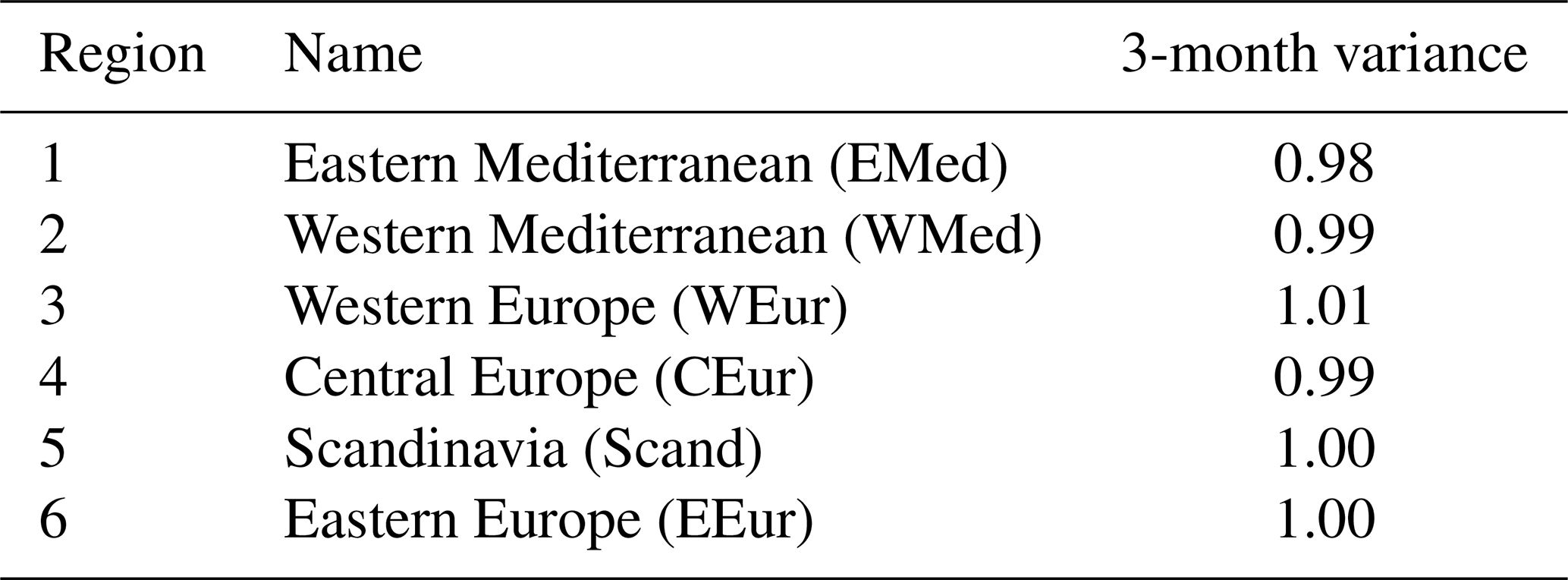
In this study, the term |x₁(t)∩x₂(t)| expresses the number of time steps where both timeseries are equal to 1, while the term |x₁(t)∪x₂(t)| denotes the total number of time steps. The distance coefficient can be rewritten using the Jaccard coefficient, as defined by Jaccard (1912), denoted by J(x₁,x₂). This metric highlights the synchronicity of time series and is therefore particularly appropriate to create regions with similar drought behavior. The UPGMA algorithm is initialized by taking the total region, which it then subdivides into two regions for which the metrics are similar. At each iteration, it increases the number of clusters by one, by optimally subdividing one of the regions defined at the previous iteration. The algorithm stops when the set of defined regions corresponds to the grid points. A compromise must therefore be found between the number of regions, their sizes, and the synchronicity of the time series within these regions. After applying this algorithm and studying the proposed regional breakdowns, we have decided to retain six regions. This choice, though somewhat arbitrary, was considered suitable for our objectives. Conventional clustering criteria did not provide a clear basis for selecting an optimal number of regions, and moderate variations in this number would not have substantially affected our findings. The regionalization is illustrated in Fig. 1. To judge the relevance of this division, we check that the seasonal variance of SPI3 (as defined in the previous section) averaged over all regions remains within the interval [0,1]. The variance of the SPI3 averaged over each region is not different from 1 at the 95 % confidence level, which confirms the suitability of the regionalization for the purpose of this study. The names of these regions and their variance are presented in Table 1.

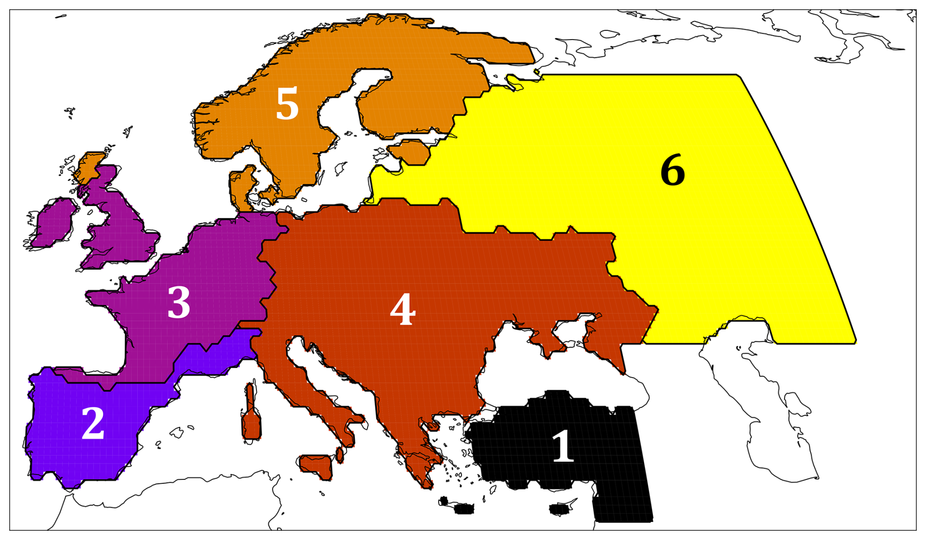
Figure 1 Regionalization of Europe derived from seasonal drought concurrence (see text for details).

Table 1 Region names and mean SPI3 variances.

It should be noted that these regions are very similar to those obtained in other studies. Stefanon et al. (2012) or Pyrina and Domeisen (2023) propose a clustering of their data (heatwaves and heat extremes) above their region of interest. The clusters obtained have a variable geographical centre of action, suggesting different behaviours with regard to the variables in each of the areas located below the centre of action.

2.2.3 Identifying drought events

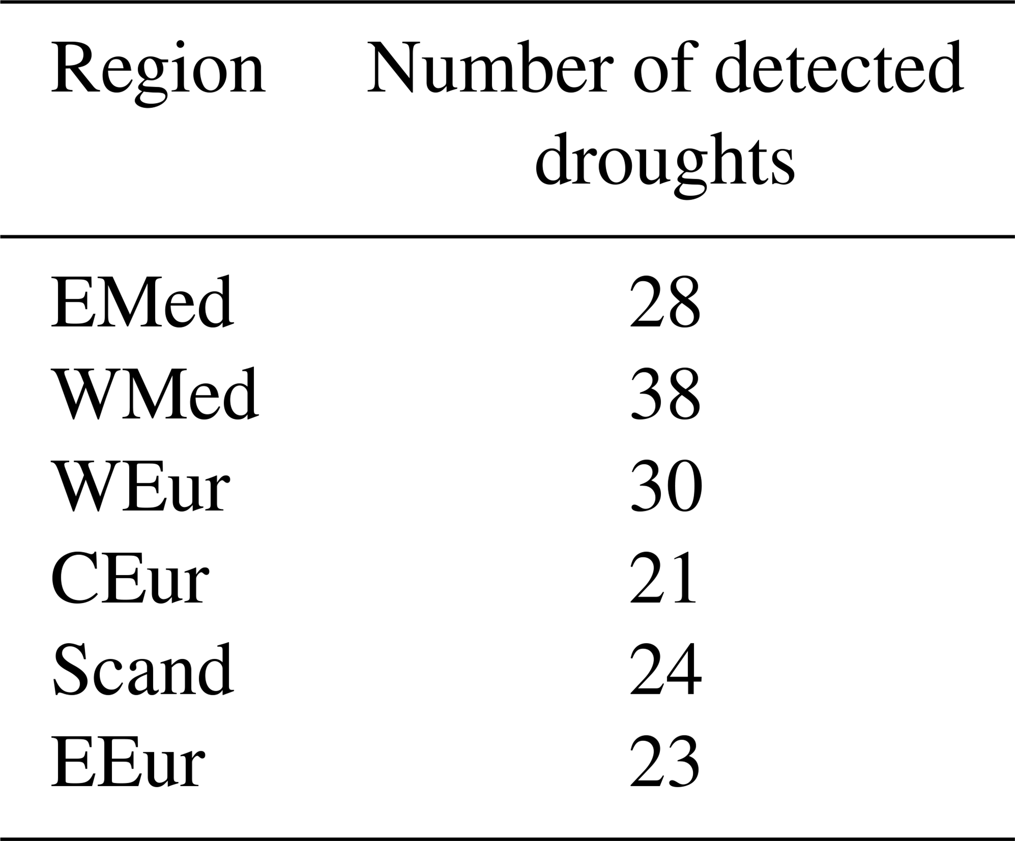
Having defined these new regions, we then consider a region to be dry if its spatially-averaged SPI3 falls below the value −0.84. Further, droughts lasting 10 d or less have been excluded in order to retain relatively long events only. In most studies (Spinoni et al., 2019, 2014), SPI is calculated on a monthly rather than daily timescale, which means that the SPI calculation, regardless of the running integration period, is based on monthly precipitation anomalies over the entire period rather than daily precipitation anomalies. The droughts considered persistent are usually those lasting more than 2 months. Here, we compute the SPI3 at a daily timescale and if two droughts are separated by less than 3 months, then we consider that it is the same event, consistently with the use of the SPI3. Each drought is associated with a time stamp corresponding to the minimum SPI3 over the drought period. The Fig. 2 presents the spatially averaged timeseries of SPI3 over one of the previously defined regions (see Sect. 2.2.2). Dry spells (SPI3 less than −0.84) are shown in dark red. For each drought period, the red dotted vertical line indicates the local minimum SPI3 corresponding to its reference date. For each region, the number of droughts identified over the 1960–2022 period is presented in Table 2.

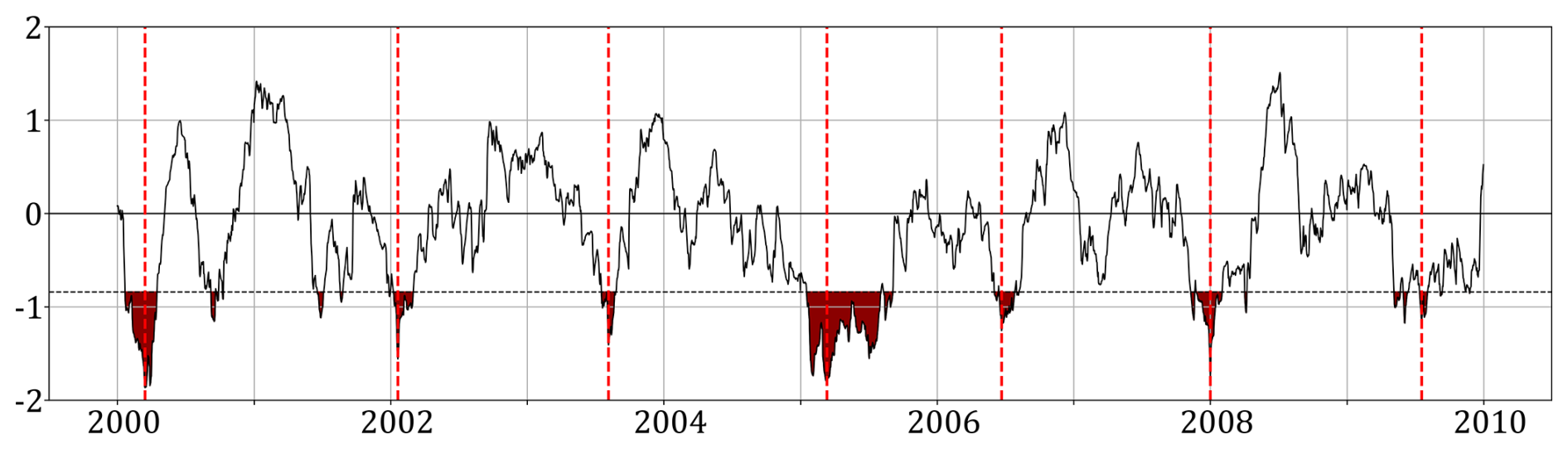
Figure 2 Drought characterization principle: the SPI3 time series (here for the Western Mediterranean region) is used to detect droughts by selecting periods for which the SPI3 is less than −0.84. The vertical red line shows the minimum of the SPI for the detected drought, corresponding to the day where the maximum intensity of the drought is reached.

Table 2 Number of detected droughts over 1960–2022, for each region.

2.2.4 Weather regimes

The year-round weather regimes are obtained following a procedure very similar to that presented in Grams et al. (2017). The main difference is the size of the domain, since we wanted a slightly larger domain covering our full study area, including the EEur region. Weather regimes are computed from daily 500 hPa geopotential height (zg500) over the 1991–2020 period. The pre-processing and clustering steps are described hereafter. The climatology of daily zg500 is calculated and smoothed by interpolating a periodic spline at each grid point. This climatology is then removed from the raw signal to obtain the zg500 anomalies. A linear regression is also used to remove the temporal trend (computed over the spatially-averaged signal) over the 1991–2020 period. This is to remove the effect of thermal expansion of the lower troposphere, which can distort the distance metrics used by the classification even though it does not reflect a circulation effect. We then apply a low-pass filter to the anomalies, in the form of a 5 d moving average. The variance of zg500 at mid-latitudes being larger in winter than in summer, the normalization of zg500 anomalies requires to remove this seasonality. Disregarding this seasonal difference in variability may result in a spurious predominance of winter weather regimes. Normalization is obtained by dividing the daily filtered anomalies at each grid point by the same calendar scalar index. This index is calculated by computing the standard deviation of the zg500 signal over a sliding window of 30 d, for each day of the year and at each grid point, and then spatially averaging over the domain.

We then reduce the dimensionality by determining the first empirical orthogonal function (EOFs) of the previously computed zg500 anomaly time series (Wilks, 2019) and their associated principal components (PCs). This fonction take into account a weighting by the cosine of the latitude. We retain a minimum of 90 % of the total variance, which leads to keep the first 13 components of the signal. The time-averaged spatial correlation coefficient between the reconstructed daily zg500 anomaly maps (sum of all the retained EOFs multiplied by their respective PCs) and the initial signal is 0.95, which also validates our choice.

Finally, the weather regimes are obtained by clustering the PCs using the k-means algorithm. The number of clusters is arbitrary, but can be oriented using several metrics (Lee et al., 2023). We applied these metrics to our case study (see discussions in Sect. S1 in the Supplement), but we found that there is no optimal number of weather regimes. We chose to retain 7 clusters in order to align with the existing literature (Grams et al., 2017; Büeler et al., 2021).

The centroids are calculated over the reference period (1991–2020) and then each day of the study period (1960–2022) is assigned to a centroid. To do so, we project the 1960–2022 daily zg500 detrended anomalies in the 1991–2020 PCs space and then compute the Euclidean distance to each of the centroid. To reassign WRs to each day of this longer period, we project the daily zg500 anomaly in the PCs space and then compute the Euclidean distance to each of the WR. The attributed WR is the one presenting the minimum distance. If the distance is too high for each WR (distance superior to 4.5, chosen to retain approximately 20 % of WR0), we attribute the “no regime” WR to this day (or “Weather regime 0”). Further, we apply a persistence criterion to retain sequences of at least 4 d in the same regime. Leftover days are assigned to the additional regime “WR0”, accounting for transition between canonical regimes. The resulting weather regimes, expressed as zg500 anomaly composites, are illustrated in Fig. 3. The analysis yields weather regimes designated as the Zonal Regime (ZO), the Greenland Blocking (GBL), the European Blocking (EuBL), the Atlantic Ridge (AR), the Atlantic Trough (AT), the Mediterranean Trough (MTr), and the Scandinavian Blocking (ScBL). These results are mostly consistent with WRs obtained by Grams et al. (2017) and Büeler et al. (2021). We can attribute discrepancies with these studies to the use of ERA5 instead of Era Interim, and by a slightly different spatial domain (75° W to 64° E and 28 to 75° N as opposed to 80° W to 40° E and 30 to 90° N, chosen larger to include all the EEU AR6 regions), and time period (1991–2020 vs. 1979–2015 for Grams et al., 2017 and 1997–2017 for Büeler et al., 2021). We obtain a new WR “Mediterranean trough”, characterised by an anticyclonic anomaly in northern Europe and a cyclonic anomaly over the Mediterranean. This pattern probably arises from the extended spatial domain to the east, which allows a zonal wave structure to appear over eastern Europe and thus a stationary anomaly over the Mediterranean.

Figure 3 Composite zg500 (contours) and zg500 anomalies (color shades) for each weather regime, and their associated frequency (in %), calculated over the reference period (1960–2022). Isolines are shown every 65 gpm.

The weather regimes presented here are ranked in descending order of frequency over the entire period, irrespective of season. Section S2 shows, for each day of the year, the mean frequency of each WR. The seasonal predominance of these weather regimes is consistent with the findings of Büeler et al. (2021). There is a more homogeneous frequency distribution of weather regimes in winter than in summer, but a winter predominance of cyclonic weather regimes and a summer predominance of blocking weather regimes. The zonal regime is found to be the most frequent, with an occurrence frequency of 14.7 %. These averaged frequencies mask multi-decadal variations affecting large-scale circulation. We discussed this point in Sect. 4.2.

The precipitation anomaly pattern associated to a given weather regime is obtained by averaging the precipitation anomalies of all the days assigned to that weather regime. The resulting composite patterns are shown in Fig. 4. Precipitation composites show strong and coherent signals, thereby justifying the use of year-round regimes in our analysis. Large-scale patterns of precipitation anomalies were expected, in association with large-scale regimes. Overall, anti-cyclonic weather regimes are associated with negative precipitation anomalies in the high-pressure regions, while low-pressure regions induce positive precipitation anomalies.

Figure 4 Average precipitation field (composite) for each weather regime. Non-significant results (p value > 0.05) are hatched.

As demonstrated in Fig. B1 in the appendix, the precipitation signature associated to year-round weather regimes (with respect to seasonal climatologies) is relatively stable across seasons. Yet, a few noticeable differences are worth mentioning: The most striking differences are the shifts between dry winter (DJF) and wet summer (JJA) anomaly over southwestern Europe for EuBL and conversely for AT. Another seasonal change is the dampening of the wet-north dry-south contrast (resp. wet-southeast dry-southwest) between winter and summer for ZO (resp. AR). Finally, MTr and ScBL wet patterns show a stronger amplitude in Autumn, possibly due to seasonal heavy precipitation events affecting the Mediterranean and surrounding regions.

The ZO and EuBL regimes exhibit a more pronounced precipitation contrast during winter months compared to summer months. Similarly, the AT regime yields much drier anomalies in summer than in winter over Southwestern Europe, while the same phenomenon is observed for the AR regime over the JJA and SON periods. These differences require to quantify the error made when considering a single precipitation pattern per regime, rather than four per regime (one per season). This question is discussed in Sect. 4.3

2.2.5 Drought reconstruction informed by weather regimes

In order to quantify the contribution of weather regimes to the precipitation deficit leading to droughts, we calculate for each region the average frequency of each weather regime during the 91 d preceding the droughts. We can then compute the part of the precipitation anomaly that can be explained by an anomaly in the frequency of occurrence of each weather regime.

For each region, we aim to reconstruct the averaged precipitation anomaly $\stackrel{\mathrm{‾}}{p_s}$, computed over all periods of 91 d that precede droughts. The duration of this period is intended to cover the SPI3 integration window, i.e. 3 months. One can get the mathematical expression of $\stackrel{\mathrm{‾}}{p_s}$ using the following decomposition. We first categorize the ensemble of days Ω, into 8 weather regimes k (counting the regime 0) so that Ω = ⋃_k Ω_k. On the entire period we have :

• The climatological frequency of the weather regime k:

  $$f_k={\displaystyle \frac{n_k}{N}},$$

  where n_k is the number of days in the WR k, and N the total number of days in Ω, so that $\sum _k{n}_k$ = N and $\sum _k{f}_k$ = 1.

• The canonical precipitation anomaly pattern of the WR k:

  $$\begin{array}{}\text{(2)}& C_k={\displaystyle \frac{\mathrm{1}}{n_k}}\sum _{d\in {\mathrm{\Omega }}_k}{p}_{\mathrm{d}}\end{array}$$

  which are the mean precipitation anomaly pattern when in WR k (shown in Fig. 4), with p_d the daily precipitation anomaly.

On the subset of N^S days that precede droughts (here, N^S = 91 × N_droughts days), we have

• The frequency of the WR k:

  $$f_k^S={\displaystyle \frac{n_k^S}{N^S}},$$

  where $n_k^S$ is the number of days in the WR k throughout the 91 d periods that precede droughts, with $\sum _k{n}_k^S$ = N^S.

• The precipitation anomaly pattern of the WR k during this period:

  $$\begin{array}{}\text{(3)}& C_k^S={\displaystyle \frac{\mathrm{1}}{n_k^S}}\sum _{d\in {\mathrm{\Omega }}_k^S}{p}_{\mathrm{d}}\end{array}$$

  with ${\mathrm{\Omega }}_k^S$ = Ω^S⋂Ω_k.

By construction, precipitation anomalies $\stackrel{\mathrm{‾}}{p}$ verify $\stackrel{\mathrm{‾}}{p}$ = 0 and write as follows:

$$\begin{array}{}\text{(4)}& \begin{array}{rl}\stackrel{\mathrm{‾}}{p}& ={\displaystyle \frac{\mathrm{1}}{N}}\sum _{d\in \mathrm{\Omega }}{p}_{\mathrm{d}}\\ & =\sum _k\sum _{d\in {\mathrm{\Omega }}_k}{\displaystyle \frac{\mathrm{1}}{n_k}}{\displaystyle \frac{n_k}{N}}{p}_{\mathrm{d}}\\ & =\sum _k{f}_k{C}_k\end{array}\end{array}$$

Similarly, on the drought-preceding periods S:

$$\begin{array}{}\text{(5)}& {\stackrel{\mathrm{‾}}{p}}^S={\displaystyle }\sum _k{f}_k^S{C}_k^S\end{array}$$

Hence, the difference between the precipitation anomalies preceding droughts and climatological precipitation anomalies is (using Eqs. 4 and 5):

$$\begin{array}{}\text{(6)}& {\stackrel{\mathrm{‾}}{p}}^S-\stackrel{\mathrm{‾}}{p}=\sum _k{f}_k^S{C}_k^S-\sum _k{f}_k{C}_k\end{array}$$

So, by using

$$\begin{array}{}\text{(7)}& \mathrm{\Delta }{f}_k=f_k^S-f_k\end{array}$$

and

$$\begin{array}{}\text{(8)}& \mathrm{\Delta }{C}_k=C_k^S-C_k\end{array}$$

we can rewrite Eq. (6) such that

$$\begin{array}{}\text{(9)}& {\stackrel{\mathrm{‾}}{p}}^S=\sum _k\left[\left(f_k+\mathrm{\Delta }{f}_k\right)\left(C_k+\mathrm{\Delta }{C}_k\right)-f_k{C}_k\right]\end{array}$$

Ultimately we obtain the expression of the precipitation anomalies preceding droughts as a function of the variation of frequency anomalies and variation of precipitation patterns:

$$\begin{array}{}\text{(10)}& {\stackrel{\mathrm{‾}}{p}}^S=\sum _k\mathrm{\Delta }{f}_k{C}_k+\sum _k{f}_k\mathrm{\Delta }{C}_k+\sum _k\mathrm{\Delta }{f}_k\mathrm{\Delta }{C}_k\end{array}$$

The term $\sum _k\mathrm{\Delta }{f}_k{C}_k$ reflect the contribution of the anomalous WR frequencies that influences the precipitation. The $\sum _k{f}_k\mathrm{\Delta }{C}_k$ term characterizes the departure from the canonical precipitation patterns in periods preceding droughts. The third term can be interpreted as the interaction between patterns departure and anomalous WR frequencies. Hence, we can see this method as a way to use these frequencies to weight and cumulate each of the precipitation maps associated with the weather regimes. This entire process is illustrated in Fig. 5. Please note that the WR0 is not taken into account in the reconstruction but whose days are nevertheless taken into account when calculating the average precipitation anomalies.

Figure 5 Flowchart showcasing the methodology to reconstruct meteorological droughts over the Western Europe region (highlighted with red contours) derived from frequency anomalies of weather regimes. The bottom-right maps illustrate the comparison between the reconstructed and actual mean precipitation anomaly associated to Western Europe droughts. For simplicity, this illustration displays only four weather regimes out of the seven regimes used for the reconstruction.

In the following sections, we quantify the suitability of WRs to reconstruct precipitation anomalies by computing spatial average over the all domain of the three terms $\sum _k\mathrm{\Delta }{f}_k{C}_k$, $\sum _k{f}_k\mathrm{\Delta }{C}_k$ and $\sum _k\mathrm{\Delta }{f}_k\mathrm{\Delta }{C}_k$. In order to assess their relative contribution to the original precipitation anomalies, we normalize these terms by the precipitation anomalies computed over the 91 d preceding droughts:

$$\begin{array}{}\text{(11)}& \mathrm{1}=\underset{{\mathit{\alpha }}_{\mathrm{1}}}{\underbrace{{\displaystyle \frac{\langle \sum _k\mathrm{\Delta }{f}_k{C}_k\rangle }{\langle {\stackrel{\mathrm{‾}}{p}}^S\rangle }}}}+\underset{{\mathit{\alpha }}_{\mathrm{2}}}{\underbrace{{\displaystyle \frac{\langle \sum _k{f}_k\mathrm{\Delta }{C}_k\rangle }{\langle {\stackrel{\mathrm{‾}}{p}}^S\rangle }}}}+\underset{{\mathit{\alpha }}_{\mathrm{3}}}{\underbrace{{\displaystyle \frac{\langle \sum _k\mathrm{\Delta }{f}_k\mathrm{\Delta }{C}_k\rangle }{\langle {\stackrel{\mathrm{‾}}{p}}^S\rangle }}}},\end{array}$$

where 〈⋅〉 denotes spatial averaging. The sum of the terms is always 1. Taking Eq. (11), we can rewrite it as a sum of three scalars:

$$\begin{array}{}\text{(12)}& \mathrm{1}={\mathit{\alpha }}_{\mathrm{1}}+{\mathit{\alpha }}_{\mathrm{2}}+{\mathit{\alpha }}_{\mathrm{3}}\end{array}$$

Therefore, for the first term to predominate over the other two, we can arbitrarily set the criterion that the weather regimes explain an important part of the drought when

$$\begin{array}{}\text{(13)}& {\mathit{\alpha }}_{\mathrm{1}}>\mathrm{0}\end{array}$$

In those case, we can verify that α₁ > α₂ and α₁ > α₃ for most of the droughts. We can therefore consider that the frequency anomalies of WRs influences droughts when α > 0.33.

3 Results

3.1 Average precipitation anomalies reconstructed from WRs

For each region, we analyse the sequences of WRs during the 91 d period before the peak day of the identified droughts, as detailed in Sect. 2.2.5. The occurrence anomalies of each regime with uncertainties, for each region, are presented in Fig. 6.

Figure 6 Difference in frequency of occurrence of each regime between the period of 91 d preceding the droughts in each region and the climatological frequency of occurrence independant of drought.

The droughts in each of these regions are characterized by a significant frequency anomaly for at least five weather regimes out of seven. Overall, the confidence interval associated with each frequency anomaly is of the order of 4 %. The presence of a clear frequency anomaly signal confirms the influence of weather regimes on droughts in these regions. In addition, the differences between regions suggest that this influence is diverse across Europe, which further justifies our spatial breakdown of the continent (see Sect. 2.2.2).

For each region, the decomposition of the precipitation anomalies associated with droughts into the three terms α₁, α₂ and α₃ of Eq. (11) is shown in Fig. 7. The right column (column V) presents the normalized spatial average of each of the three terms.

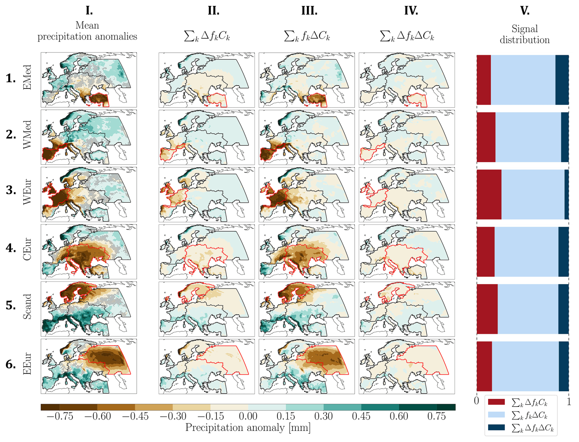
Figure 7 (I) Composite precipitation anomaly over the 3 months preceding the droughts for each region. Non-significant results (p value > 0.05) are hatched. (II to IV) Precipitation anomaly reconstructed by each term of Eq. (10) and (V) relative contribution of each term to the total precipitation anomaly.

On average, the f_kΔC_k term (i.e. α₂) dominates (Fig. 7III). For all the regions, this term reproduces a large fraction of the dry anomaly over the region of interest, then the amplitude of the signal decreases with the distance to the dried region. This term shows the departure of the precipitation pattern associated to WRs ahead of drought events compared with the canonical situations shown in Fig. 4. The strength of the signal over the dry region and its attenuation elsewhere shows that precipitation during droughts is abnormally dry compared with climatological precipitation.

The Δf_kC_k term, i.e. α₁ (Fig. 7II) is relatively small in all the regions, on average. The signal distribution (Fig. 7V) shows that the contribution of the Δf_kC_k term is slightly larger for the three regions bordering the Atlantic Ocean (WEur, WMed, Scand). Conversely, the regions the most distant from the North Atlantic EEur and EMed exhibit the lowest contribution of this term to the precipitation anomaly. Despite the low amplitude of the reconstructed signal, the precipitation pattern for this term is relatively accurate to the mean precipitation anomalies. For example, in the case of the WEur region (Fig. 7-3.II), the East-West gradient of precipitation is well reconstructed with a maximum signal amplitude over the region of interest. Although the weather regimes have large-scale canonical precipitation patterns, in some particular cases the reconstruction of the precipitation anomaly can nevertheless capture small-scale features: for the WEur region, the reconstruction captures the wet zone over eastern Spain with a maximum of dry intensity over the province of La Coruña. A special case is the reconstruction over the EEur region, which proposes a dry anomaly over the region of interest, but extends it to the rest of northern Europe. In this way, the reconstructed pattern resembles the reconstructed pattern for the Scand region. This stems from similarities in the frequency anomalies of WRs preceding droughts in these regions, with the AT, MTr and ScBL regimes being overrepresented.

The Δf_kΔC_k term, i.e. α₃ (see column IV of 7) is weak whatever the region. While less straightforward to interpret, this term can be understood as the departure of the canonical precipitation pattern occurring when the associated WR is abnormally frequent. Thus, the weak amplitude of this term can be explained by considering that this is a 2nd order term, expected to be less powerful than the other one. The sum of the three terms is not exactly equal to the composite precipitation anomalies over the three months (see Fig. 7-I).

Therefore, when averaging out over all the drought events, most of the precipitation deficit signal comes from a departure from of the canonical pattern of the WRs, and conversely, a reduced fraction can be attributed to the change in their frequency. However, for the latter contribution, we have shown that the shape of the original signal is reproduced despite a weak amplitude. This might be a consequence of averaging out over many drought events, which could conceal a variety of situations. In the next section (see Sect. 3.2), we analyse the relative contributions of the three terms for each individual drought event, rather than on average over all droughts.

While this analysis has been carried for all six regions, the following section only shows the results for the WEur region for the sake of brevity. The results for the other regions can be found in the appendix.

3.2 WR contribution to individual droughts

Figure 8 shows the distribution of the signal between the three terms α₁, α₂ and α₃ for each of the droughts detected over the example of the WEur region. Negative values indicate that the contribution of the concerned term is of opposite sign to the actual precipitation anomaly (e.g. a wet contribution to a dry anomaly). Table 3 shows, for each region, the percentage of droughts for which the contribution of anomalous WR frequencies is relatively high, i.e. that fulfill the criterion α₁ > 0.33 (see Sect. 2.2: Methods). The right column shows the number of droughts that fulfill this criterion over the number of detected droughts in this region.

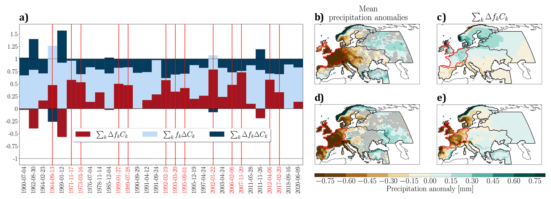
Figure 8 (a) Precipitation anomalies signal distribution for each droughts of the region WEur, red vertical lines highlighting well reconstructed droughts. (b) Precipitation anomalies averaged over the 91 d preceding droughts, for all cases where droughts cannot be explained with year-round weather-regimes. (c) Mean reconstruction's first term. (d, e) Same for all cases where droughts can be explained with year-round weather-regimes.

Table 3 (Center) Percentage of drought for which α₁ > 0.33. (Right) Number of drought for which α₁ > 0.33 over the total number of detected droughts.

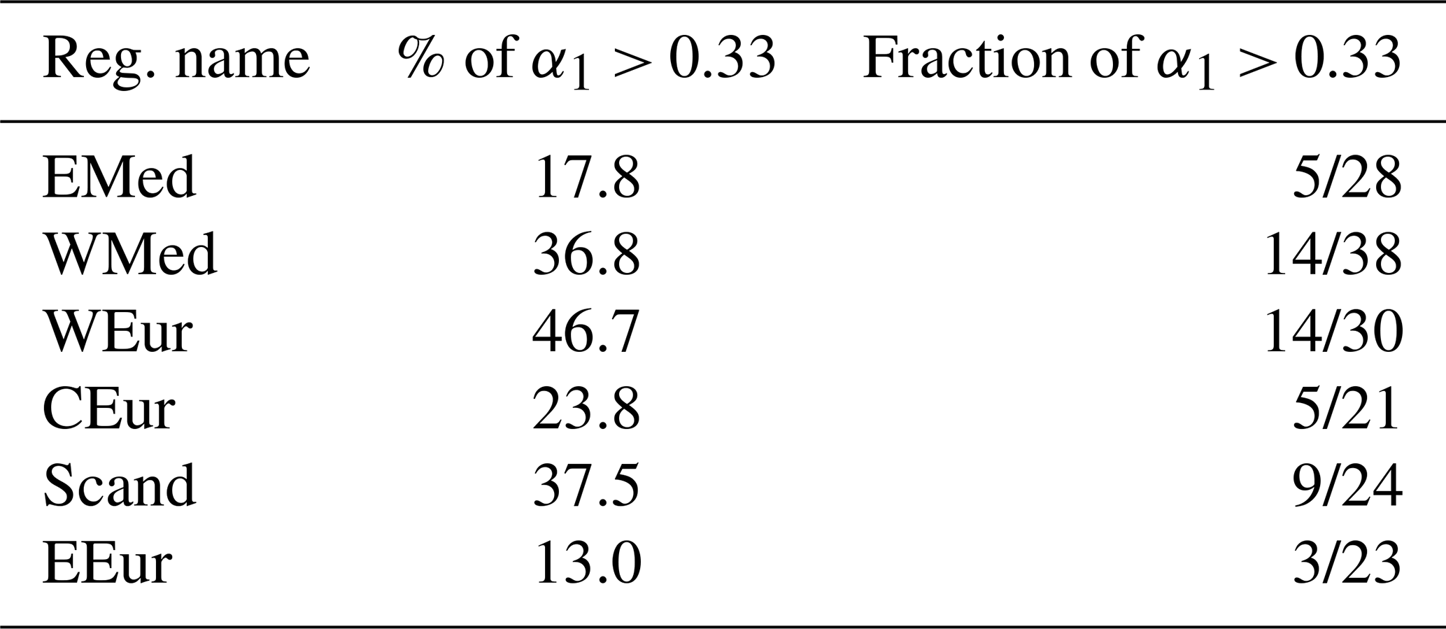
WEur, WMed and Scand are the regions with the higher percentage of droughts that can be explained by the WR frequencies. Those western regions are the ones in which the droughts are the most influenced by the large-scale atmospheric circulation in the North-Atlantic. The EMed region and EEur are the two regions in which the droughts are the least influenced by the large-scale atmospheric circulation, since only 17.8 % and 13.0 % of their respective droughts are substantially explained by anomalous WR frequencies.

For these two categories of droughts, the dry pattern is very similar, but with a slight eastward extension in the case of droughts that cannot be explained by WR. About 50 % of droughts in the WEur region can be explained by anomalies in WR frequency, in the sense of α₁ > 0.33. In these cases, the average dry pattern is well reconstructed and is characterized by a dry anomaly extending southwards to a large part of the Iberian Peninsula. The reconstructed pattern correctly captures medium-scale details, such as the rainfall anomaly over eastern Spain and eastern Italy. The explanation provided by the weather regimes therefore provides a satisfactory understanding of the dry anomaly.

For cases poorly captured by the anomalies of WR frequencies, the reconstruction shows a north-south gradient of reconstructed precipitation, which does not correspond to the actual dry anomalies. The region of interest is even reconstructed with a slightly wet anomaly. This can be seen in Fig. 8e, by observing that the α₁ signal is either very weak or negative in such cases.

3.3 Frequency anomalies

We have just shown that nearly 50 % of the WEur droughts can be satisfactorily reconstructed through the frequency anomaly of WRs (Fig. 8e). Figure 9 shows these frequency anomalies for each of the WRs, calculated for the droughts for which the WR contribution is not substantial (columns I and III of Fig. 7) or substantial (columns II and IV of Fig. 7) for the WEur region, while Sect. S3 shows the same results for all regions. Figure 9 illustrates the fact that the droughts for which the Δf_k signal is predominant are also the droughts for which the weather regimes have a well-marked frequency anomaly. The confidence interval associated with droughts where the ΔC_k term dominates does not allow us to conclude on any significant WR frequency anomaly. Therefore, these droughts are not mainly triggered by the anomalous occurrence of WRs. Section S3 shows similar results for all the other regions. All of the regions shows no significant frequency anomaly for droughts for which the Δf_k signal is not predominant. Some of them are significant but with a very low amplitude. The Scandinavian region, for instance, shows significant anomalies but with a maximum amplitude of 10 %, and with an uncertainty of ±7 %.

Figure 9 (a) Frequency anomaly of WRs in the 90 d preceding WEur droughts where the α₂ or α₃ terms are predominant (α₁ ≤ 0.33). (b) Same as (a) for droughts where α₁ > 0.33.

Signs of the frequency anomalies shown in Fig. 9b are the same as the average frequency anomalies over all the droughts, but with a stronger signal. This suggests that regime frequency anomalies are informative, but only really contribute to drought (i.e. precipitation deficit) when they are sufficiently strong. Averaging over all the events (cf. previous section) leads to an attenuation of the precipitation anomaly signal. However, the shape of the signal is still there.

Seasonality can also come into play when we look at the distribution between droughts substantially explained by anomalous WR frequencies. Figure 10 shows the percentage by season of well-reconstructed droughts for all regions.

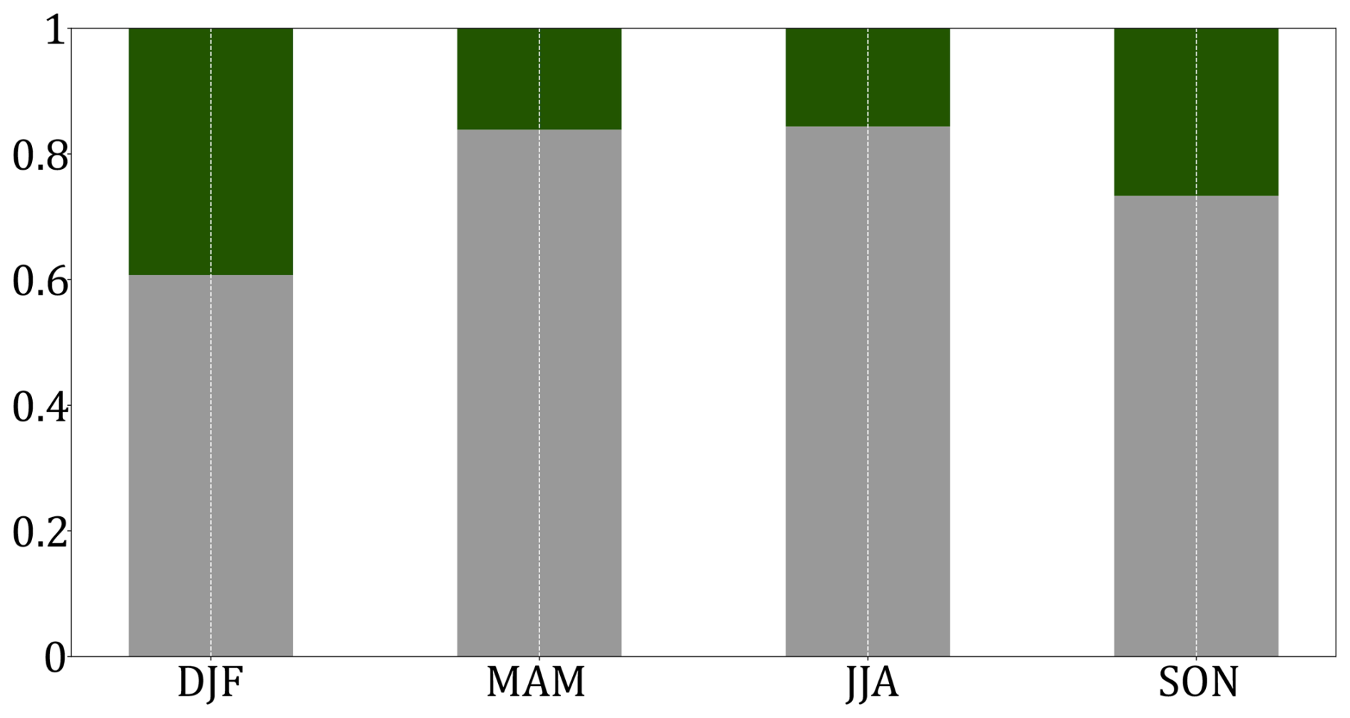
Figure 10 Average fraction of all-regions droughts explained (not explained) by large-scale atmospheric circulation through an analysis of WR frequency in green (grey).

We find that a higher fraction of winter droughts, and autumn droughts to a lesser extent can be reproduced using our weather regime approach, in contrast to spring and summer. This is consistent with the fact that the large-scale atmospheric circulation is more variable and intense in winter, with a stronger influence on the European surface weather.

4 Discussion

4.1 Further insights into the dominance of α₂

To better understand the origin of the dominant terms in ΔC_k, we examined the relationship between the daily precipitation pattern and the canonical pattern associated with the corresponding weather regime. Differences between these two patterns may arise from two joint factors: (i) the deviation of the daily zg500 field from its regime centroid, and (ii) the non-bijective relationship between a given zg500 configuration and the associated precipitation field.

To disentangle these effects, we compared, for each day, the anomalies of zg500 and precipitation relative to their respective canonical patterns (Fig. 11). Each point represents 1 d of the entire record. Points located near the upper-right quadrant and close to (1,1) indicate days when both precipitation and zg500 resemble their canonical regime patterns, whereas points near the centre correspond to days that strongly depart from them. Please note that this analysis was conducted for each days of the entire 1960–2020 period. Yet, the result remains valid during pre-drought periods (not shown).

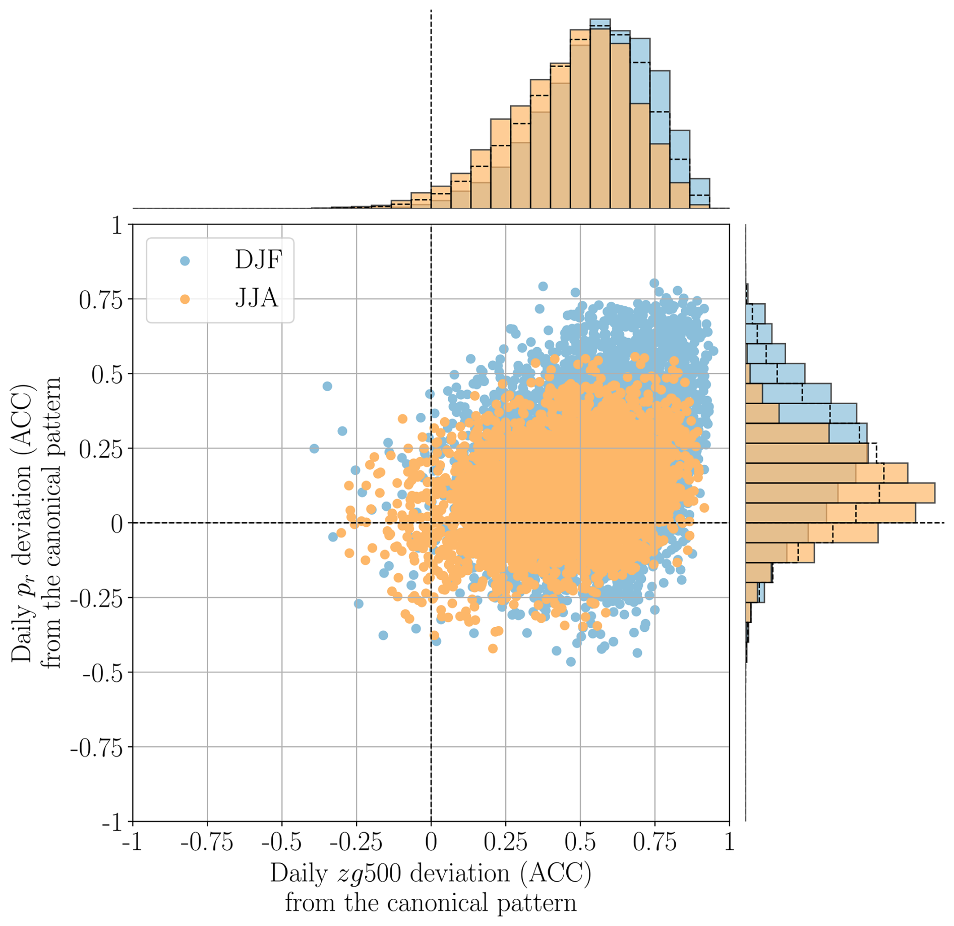
Figure 11 Scatterplot (dots) and distributions (bars) of daily anomaly correlation coefficients (ACCs) between observed fields and the centroids of their assigned weather regimes, for precipitation (y axis) and zg500 (x axis), in DJF (light blue) and JJA (orange). Days assigned to WR0 are excluded. Distribution with dotted lines are the distributions for all days.

The all-day distributions (distribution with dotted lines in Fig. 11) show that the ACC values are generally positive for zg500, in contrast to precipitation. This confirms that the daily zg500 fields assigned to a given weather regime closely match their canonical counterparts – a result expected from the clustering procedure. The median ACC for zg500 exceeds 0.5, underlining the relevance of representing large-scale circulation on an all-season timescale. Most days therefore remain relatively close to the zg500 centroid of their assigned regime.

In contrast, only a small fraction of daily precipitation fields exhibit ACC values above 0.5, and the median is below this threshold. This agrees with the findings of Sect. 3.1 and 3.2, showing that precipitation exhibits substantial variability even within a single weather regime. The contrast between precipitation and zg500 ACCs thus quantifies the strength of their coupling: when zg500 is close to its canonical pattern but precipitation is not, this reduces the representativeness of the composite precipitation pattern for that day. In such cases, precipitation anomalies appear less directly controlled by large-scale circulation.

Moreover, the distributions indicate overall higher ACCs in winter (DJF) than in summer (JJA), especially for precipitation. This implies that daily circulation patterns are more coherent in winter, making the WR framework more effective in that season. It also suggests that large-scale circulation is a stronger predictor of European precipitation anomalies during winter, while in summer, local thermodynamic processes – such as small- to meso-scale convection – likely play a more prominent role.

Similar conclusions hold when considering each weather regime separately (see Sect. S5), with particularly marked seasonal contrasts for some of them (e.g. ZO, EuBL, AR). Given that the link between precipitation and circulation seems poorly represented in some cases, we have tested an alternative method. We include in Appendix D a discussion on the use of weather regimes derived from Maximum Covariance Analysis (MCA). This approach has the advantage of identifying patterns that maximize the covariance between the zg500 field and precipitation. The resulting regimes are broadly similar to those obtained in our analysis.

A recent study (Gerighausen et al., 2025) quantifies the intra-regime variability of surface impacts more broadly, using a continuous index I_WR. Applied to precipitation anomalies, this approach could contribute to better understanding the variable importance of the term α₂ among drought events for a given region. Its application, that would involve incorporating an additional temporal dimension, goes beyond the scope of this study. Nevertheless, their method would be worth employing in future works to examine the link between life cycle parameters of weather regimes and subsequent droughts.

4.2 Non-stationarity

In this study, we computed the WR frequency anomaly relatively to a climatological frequency over the entire period, assuming stability of WRs frequencies throughout the period. This approach may conceal variations or trends in WR frequencies, with potential impacts on our results.

To verify this, we computed the 1960–2022 linear regressions on the frequencies of occurrence of WRs (see Figs. C1 and C2) and found no significant trend, except the Zonal Regime (significant correlation coefficient of 0.12) which presents a positive slope of approximately +0.5 per year.

Similarly, to test the hypothesis of an even temporal distribution of drought events over the study period, we analyzed the variations in the number of days separating two consecutive droughts across all regions (Sect. S4). No significant trend was detected (p values ranging from 0.1 to 0.7 across regions). This result supports the assumption that droughts were evenly distributed throughout the period, thereby justifying the use of an average climatological frequency for their analysis.

However, estimating non-stationarity in WR frequency or drought events using linear trends remains limited. In particular, this approach does not capture decadal variability that is potentially linked to low-frequency modes of ocean dynamics, such as the Atlantic Multidecadal Variability (Hertigand Jacobeit, 2014; Cassou et al., 2004). The possible influence of these modes of variability on the relationship between year-round WRs and European droughts remains to be investigated.

4.3 Seasonality of the reconstruction

The mean precipitation over 91 d periods is reconstructed using precipitation patterns assumed to be invariant throughout the year. However, in reality, each year-round weather regime (WR) is associated with a precipitation signature that slightly varies seasonally, which may introduce a small bias in our reconstructions. We discuss here the implications of this seasonal variability.

When reconstructing precipitation for a given region, we implicitly assumed that drought events are evenly distributed over the year. If this assumption does not hold, the reconstruction may fail to capture the seasonal component of the precipitation anomaly associated with the predominant season. For example, a given WR may correspond locally to precipitation anomalies of opposite sign in winter and summer. When averaged annually, these opposite anomalies cancel out, leading to a near-zero reconstructed anomaly. Consequently, if droughts are concentrated in a specific season, the reconstructed anomaly based on annually averaged WR precipitation patterns will tend to be underestimated.

To assess this effect, we computed the seasonally averaged precipitation signature of each WR (relative to seasonal climatologies; Fig. B1). Comparison with the annually averaged signatures (Fig. 4) allows to quantify, for each region and WR, the bias induced by the seasonality of droughts. The resulting maps (Fig. E1) show the difference between the annual and seasonal reconstructions. Negative values (red shades) indicate an underestimation of the true precipitation anomaly by the annual reconstruction method, and positive values indicate the opposite.

Three notable features emerge: (i) the row corresponding to the ScBL WR, (ii) that of the AT WR, and (iii) the column associated with the CEur region. The AT WR shows a systematic underestimation of precipitation anomalies over the northern Mediterranean. As seen in Fig. B1, the precipitation signature of this WR is weaker during MAM and JJA than during SON and DJF. Although the WR occurs throughout the year, using an annually averaged pattern leads to an underestimation of anomalies when droughts occur in autumn or winter. A similar effect is found for the ScBL WR: the underestimation of precipitation anomalies over western Europe reflects the strong seasonal variability of the ScBL precipitation signature (Fig. B1-7).

An examination of Fig. E1 by column shows that the CEur region exhibits larger biases than other regions, suggesting that drought events there are unevenly distributed through the year. The seasonal precipitation signature of the EuBL WR is markedly drier in SON and DJF, while its annually averaged pattern displays a weaker negative anomaly. This also reflects our regionalization choice: the CEur region is spatially extensive and therefore expected to show greater heterogeneity in drought patterns. This limitation stems from our decision to retain only six regions in the regionalization process.

Although the overall bias due to seasonality remains small in most cases, the quality of the reconstruction can be lower when the AT or ScBL regimes dominate the circulation during drought periods. From the perspective of the decomposition introduced in Sect. 2.2.5, this seasonal bias has direct implications for the interpretation of the terms α₁ and α₂. Because the canonical precipitation patterns C_k used in the reconstruction are computed as annual averages, they may underestimate the amplitude of precipitation anomalies for regimes whose precipitation signature is stronger during the season when droughts preferentially occur (e.g. AT or ScBL in winter). In such cases, the contribution associated with anomalous weather-regime frequencies (α₁) is likely to be underestimated.

Conversely, part of the mismatch between the actual seasonal precipitation anomalies and the annual canonical patterns is transferred to the f_kΔC_k term, leading to an overestimation of α₂. Seasonal variability in regime-related precipitation signatures may therefore shift part of the circulation-related signal from α₁ to α₂, even though both terms ultimately reflect different aspects of the circulation-precipitation relationship.

As a consequence, the dominance of α₂ identified in this study should be interpreted as an upper bound, while the contribution of α₁ should be regarded as conservative. Explicitly accounting for seasonal precipitation patterns would likely increase the relative importance of anomalous regime frequencies for regimes and regions exhibiting strong seasonal contrasts, without altering the main qualitative conclusions of this work.

5 Conclusions

The aim of this study is to quantify the strength of the relationship between low-frequency large-scale North-Atlantic atmospheric circulation and 3-month meteorological droughts over Europe. Droughts are here defined relatively to the seasonal cycle of precipitation, and can thus occur anytime within the year. We use year-round weather regimes (WRs) to assess the link between atmospheric patterns and droughts over regions obtained with a regionalization method, regardless of the season. We quantify the contribution of WR frequency anomalies in the 3-month preceding the drought to the resulting precipitation deficit. We find that the WR approach to characterize the atmospheric circulation explains only partly the development of European droughts. The strength of the signal depends strongly on the region considered, with a stronger (weaker) influence of the circulation for western (eastern) regions.

The contribution of WR frequency anomaly is important for around 50 % of drought events. It is higher for winter and autumn droughts than for summer droughts. This seasonal contrast is consistent with the fact that WRs explain precipitation variability more robustly in winter than in summer, when precipitation is more influenced by local thermodynamic and convective processes and thus less tightly constrained by large-scale circulation.

The analysis of the persistence and intensity of individual WR life cycles (Sect. S6, Figs. S6 and S8) indicates that in most cases, the frequency anomaly cannot be explained both by an increased persistence alone or an increased number of sequences alone, but rather by a combination of both.

Our findings could have substantial implications in the field of sub-seasonal to seasonal drought predictions, provided forecast models manage to capture and anticipate anomalous WR frequency (Osman et al., 2023; Ferranti et al., 2018). In our future work, we will then assess the capacity of state-of-the-art Earth system models to capture the appropriate amount of WR variability and their relation to seasonal precipitation anomalies across Europe. We will also evaluate the stability of this relationship in the context of climate change.

Appendix A: Validity of the SPI across the region

The SPI3 has been used to forecast droughts with a high level of confidence (Cancelliere et al., 2007), and to establish a climatology of drought for the European region (Gudmundsson and Seneviratne, 2015; Caloiero et al., 2018; Spinoni et al., 2017). As mentioned earlier, the SPI allows to transform the generally non-Gaussian probability density function of precipitation climatology into an index exhibiting normal/gaussian distribution properties and centered on the 0 value. However, it assumes that the probability of having a dry event with a certain intensity is the same as that of having a wet event with the same intensity. This symmetry assumption in the cumulative precipitation distribution, although generally valid, is questionable for arid regions, according to the study of (Wu et al., 2007). Yet, to our knowledge, there is no off-the-shelf method to assess the validity of this index. We thus propose two distinct methods to assess its applicability.

The first method consists of fitting a gamma distribution on 3-month precipitation and estimating the skewness parameter that characterizes its asymmetry. Since the problem of validity of the SPI arises from the asymmetric shape of the precipitation distribution, the higher the skewness the less valid the SPI. In the context of a random variable (in this case, daily precipitation), if it is observed to follow a Gamma distribution with parameters k and θ, the probability density is expressed as follows:

$$f\left(x,k,\mathit{\theta }\right)={\displaystyle \frac{x^{k-\mathrm{1}}{\text{e}}^{-\frac{x}{\mathit{\theta }}}}{\mathrm{\Gamma }\left(k\right){\mathit{\theta }}^k}}$$

for all x > 0 where k is the shape parameter and θ is the scale parameter, and Γ is Euler's Gamma function. The skewness coefficient of the distribution is $\frac{\mathrm{2}}{\sqrt{k}}$. For each season (DJF, MAM, JJA, SON) of the period, we averaged over the years all cumulative precipitation, then performed a Gamma regression on this resulting distribution, and calculated the skewness coefficient. The results are shown in the right-hand panel of Fig. A1 for the winter and summer seasons.

The second method relies on the variance of the SPI that should be close to 1 by construction (Sönmez et al., 2005). When the asymmetry of the precipitation distribution is too skewed, the normalization leads to a SPI with a variance different from 1. We thus compute at each grid point and for every season of each year the variance of the SPI3 time series. This variance is then averaged over all years, to obtain a mean value for each season. The results are displayed in Fig. A1 on the right for the winter and summer seasons. The statistical significance of the result was computed by means of a bootstrap algorithm processing 1000 resampling draws with replacement.

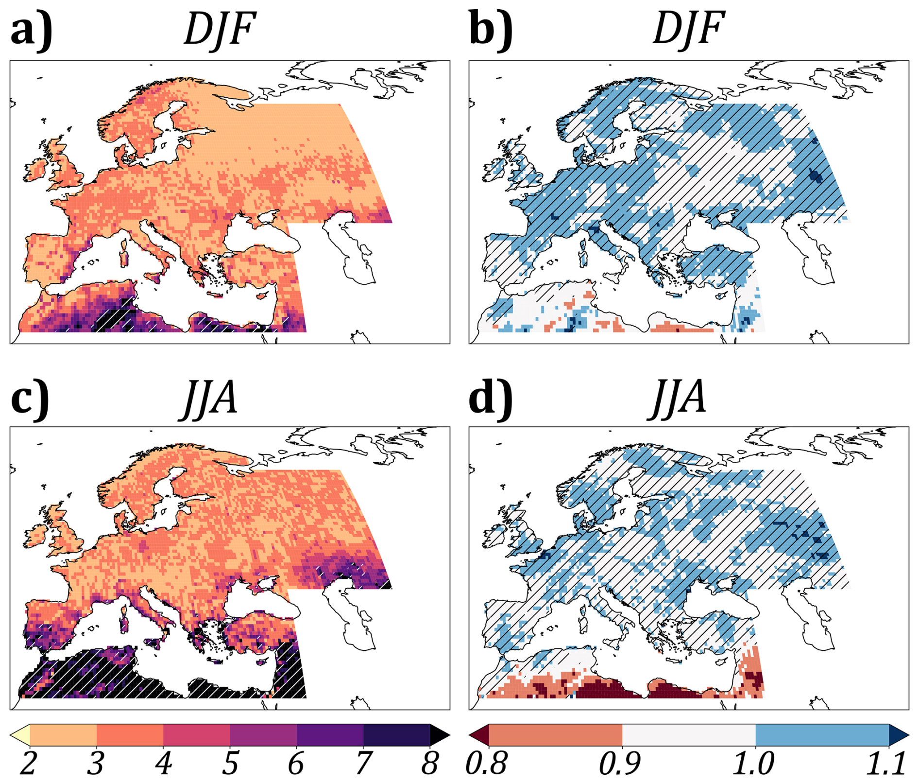
Figure A1 (a, b) Skewness coefficient of the Γ distribution fitted on precipitation data for winter (DJF) and summer (JJA). Hatching indicates a skewness coefficient significantly greater than 7 (p value < 0.05). (c, d) Variance of SPI3 in winter (DJF) and summer (JJA). Hatching indicates values not significantly different from 1 (p value < 0.05).

We find that the SPI3 variance is close to 1 (i.e. not statistically different) over most of the domain except for its southernmost part. This is confirmed by the skewness coefficient that is significantly larger than 7 in the North African and Middle East regions in summer. This questions the validity of the SPI over such regions. We thus exclude this region in the subsequent analysis and focus on a reduced domain extending from 34 to 72.6° N (see Sect.2.2.2).

There is a significant similarity between the skewness coefficient and the variance. The skewness coefficient, which is calculated before the SPI is obtained, is therefore an acceptable proxy for the validity of the SPI. However, there is no quantifiable criterion for the value of this skewness coefficient. In the context of our study, a threshold of 7 for the skewness coefficient seems appropriate. Of course, this threshold remains arbitrary and would require more rigorous demonstration in order to determine the exact value to be applied.

Appendix B

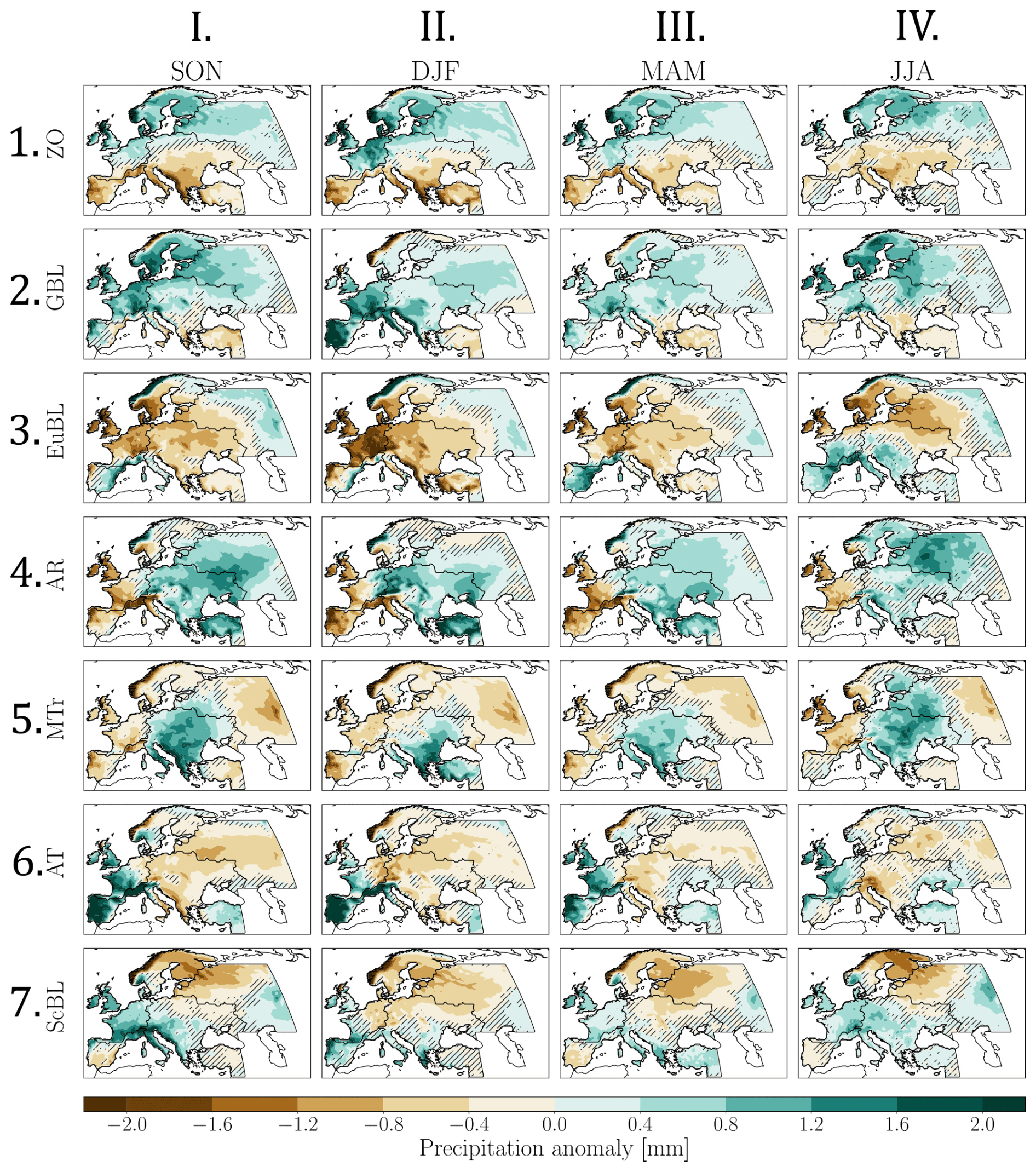
Figure B1 Seasonal precipitation anomalies (in mm) obtained for each weather regime, computed relatively to seasonal climatologies. Non-significant values (p value > 0.05) are hatched.

Appendix C

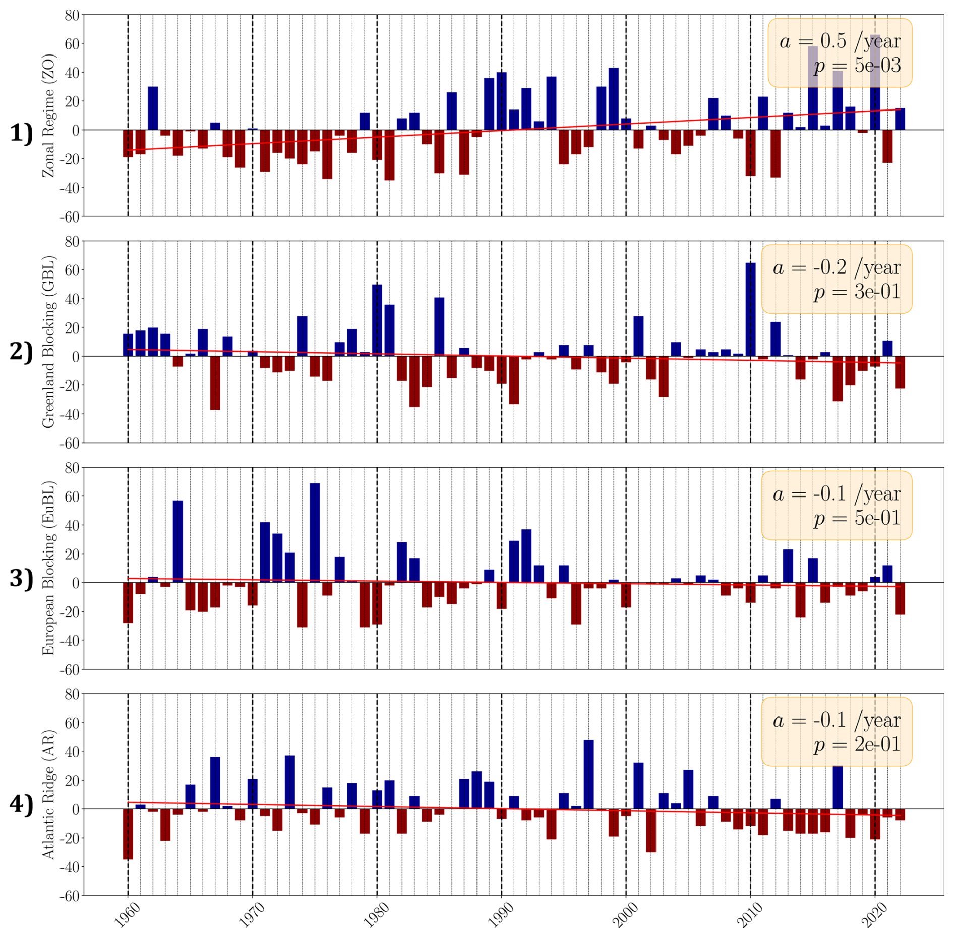
Figure C1 Annual number of days spent in the regimes, relatively to the average number of days calculated over the period 1960–2020. Linear trend obtained by regression (in red).

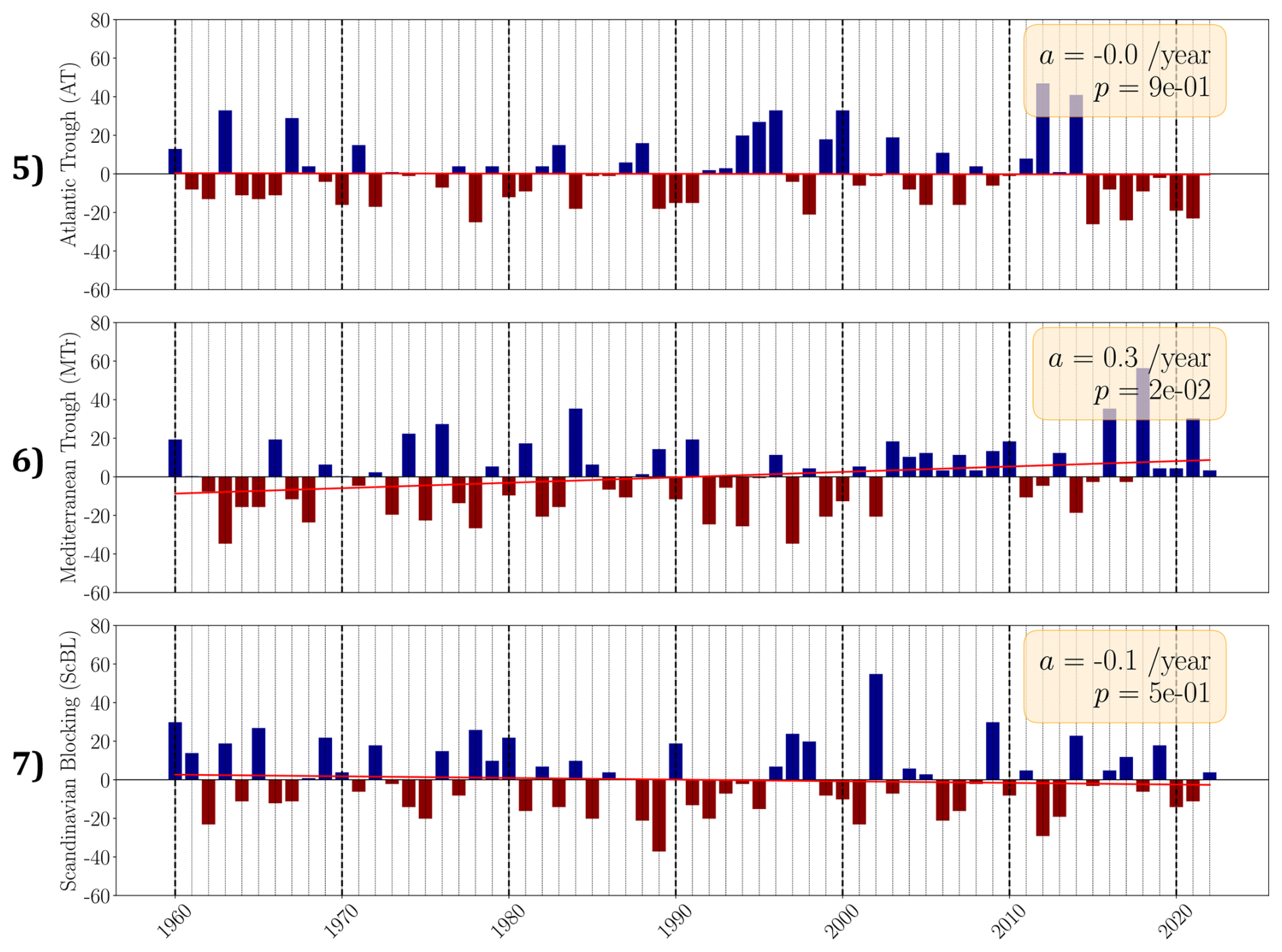
Figure C2 Annual number of days spent in the regimes, relatively to the average number of days calculated over the period 1960–2020. Linear trend obtained by regression (in red).

Appendix D: Why not MCA? An alternative set of precipitation-oriented weather regimes

The weather regimes (WRs) presented in this study are designed to represent large-scale atmospheric circulation. While this framework is effective for characterizing circulation patterns, its ability to capture the link between circulation and precipitation is limited. Because these WRs are derived solely from a PCA of the zg500 field, the resulting modes contain no explicit information about precipitation. Several recent studies have proposed alternative classification methods that focus directly on the target variable of interest (Bloomfield et al., 2020; Rouges et al., 2024; Spuler et al., 2024). One such approach is briefly outlined below.

Instead of performing a PCA to identify the leading modes of zg500 variability, a Maximum Covariance Analysis (MCA) can be applied to directly extract coupled circulation–precipitation patterns. Retaining the first ten modes (explaining 91 % of total covariability) and applying a k-means algorithm to derive seven clusters – consistent with the approach used in this study – yields a new set of seven WRs defined by joint zg500–precipitation centroids (Fig. D1).

WRs showing strong resemblance to those defined earlier are labeled with their corresponding names, while those without clear analogues are marked as “NC” (no correspondence). The degree of similarity between these MCA-based and conventional WRs provides an indication of how well circulation-based regimes alone (i.e., defined from zg500 only) capture the influence of atmospheric circulation on precipitation variability.

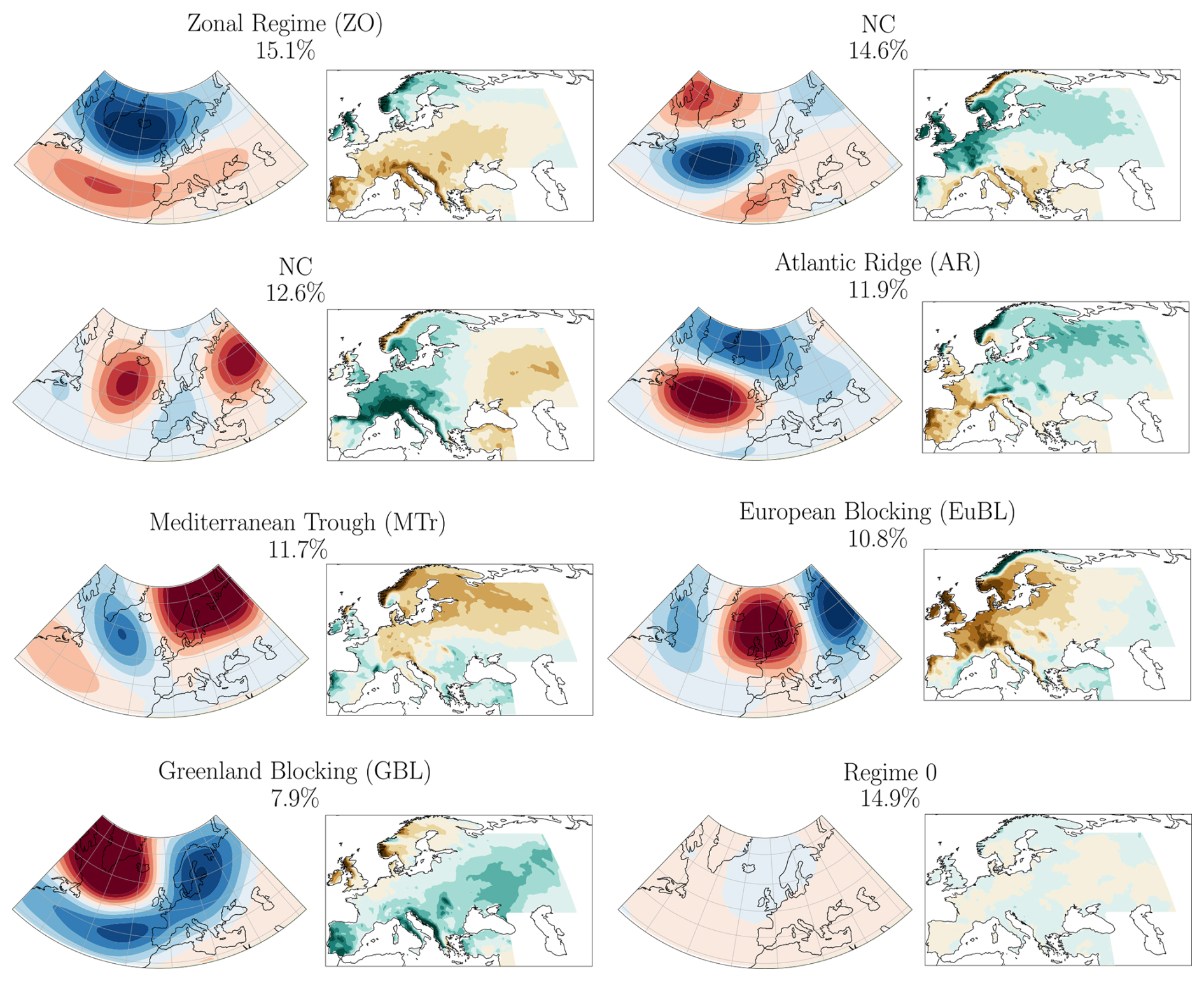
Figure D1 Composite zg500 anomalies for each new weather regime and their associated frequencies (in %), calculated over the reference period (1960–2022). The corresponding composite precipitation fields are shown for each regime.

Appendix E: Residual precipitation due to seasonality

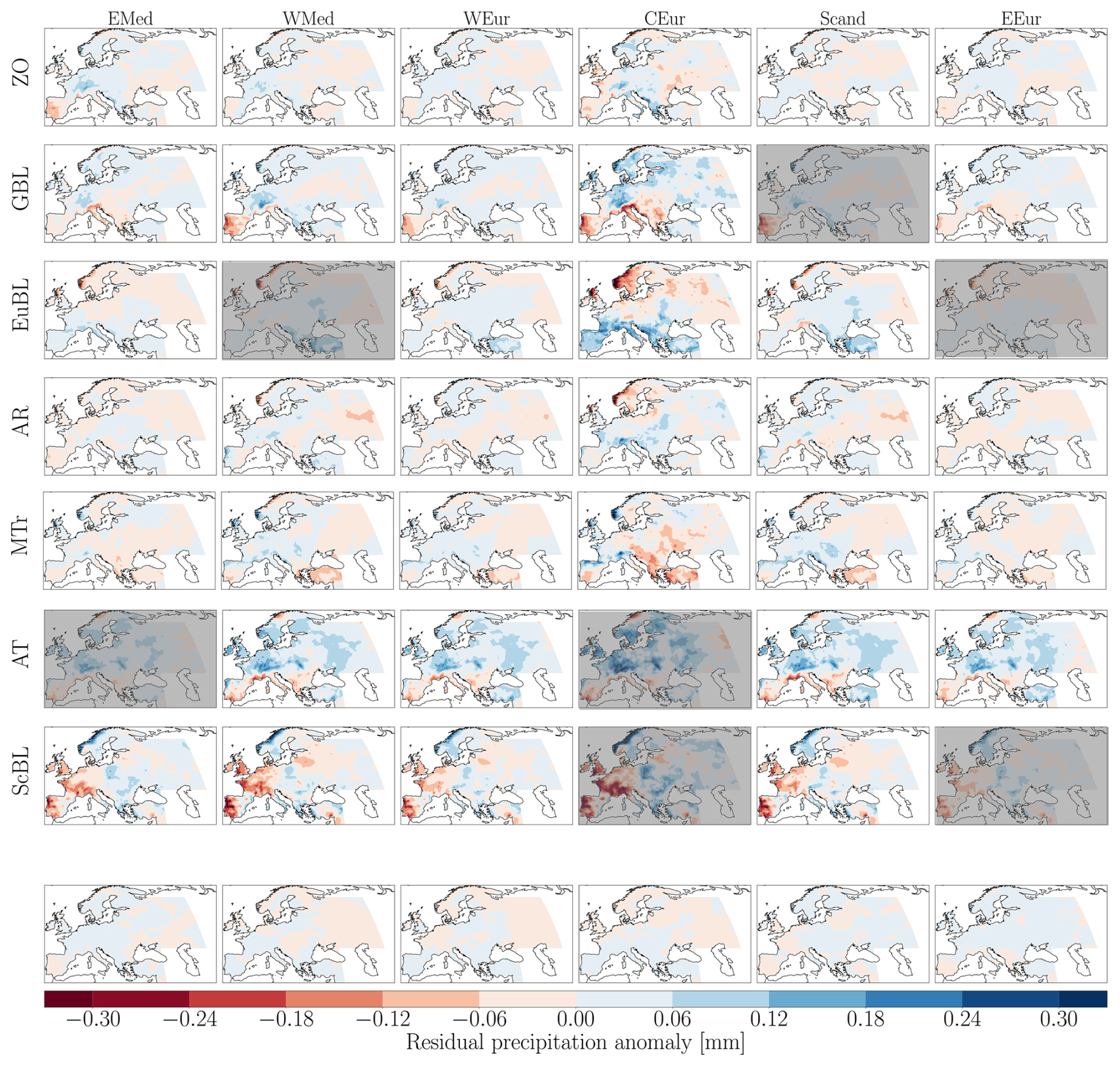
Figure E1 For each WR, difference between the composite obtained by considering an equal distribution of droughts along the year for this region, and the real composite obtained by taking into account the variation of number of droughts from one season to another. Greyed picture represents WR for which the frequency anomaly during drought is not significant. Last row of picture represent the average residual error made for each region by applying the decomposition method to the residual precipitation patterns.

For a given region, droughts are assumed to be evenly distributed throughout the year. In other words, we are not supposed to have more drought in winter than in summer. When reconstructing precipitation patterns, we use canonical patterns of regimes, i.e. average precipitation when regimes are active, regardless of the season. The precipitation patterns we use are considered to be invariant throughout the year. In reality, these precipitation patterns vary depending on the season (see Fig. B1). To be more accurate in our reconstruction, we should therefore carry out a reconstruction using seasonal patterns such as those shown in Fig. B1.

Thus, as rainfall patterns change with the seasons, we make an error when we use the average pattern for the year. The error made depends on the seasonality of droughts for a given region. Thus, for each rainfall pattern and each season, we obtain a residual rainfall that depends on the seasonality of droughts in that region.

It is possible to calculate the average residual error made for each region by applying the decomposition method to the residual precipitation patterns (see Fig. E1).