The tropospheric response to zonally asymmetric momentum torques: implications for the downward response to wave reflection and SSW events

The role of zonal structure in the stratospheric polar vortex for the surface response to weak vortex states and concurrently occurring wave reflection events is isolated using an intermediate-complexity moist general circulation model. Zonally asymmetric wave-1 momentum torques with varying longitudinal phases are transiently imposed in the stratosphere to induce stratospheric sudden warmings (SSWs) and downward wave propagation, and the subsequent tropospheric and surface response is diagnosed. The response in these torque-induced SSWs is compared to 48 spontaneous SSWs in the control experiments. Wave-1 forcings with opposite phases induce contrasting influences in the stratosphere and troposphere, including oppositely shifted polar vortex and opposite structures of wave reflection. Notably, downward wave propagation predominantly occurs over North America in the phase-90 ensemble, while primarily over North Eurasia in the phase-270 ensemble. These differences extend to surface responses: the phase-90 ensemble features pronounced cooling over Alaska and eastern Eurasia, along with enhanced rainfall concentrated over the North Pacific and North Atlantic, extending to northwest Europe. In contrast, the phase-270 ensemble exhibits significant cooling over central North America and North Eurasia, accompanied by enhanced rainfall over the North Pacific and North Atlantic, stretching into subtropical Eurasia. By analyzing the mass streamfunction of the divergent component of the meridional wind, we observe opposite-signed zonal dipole patterns between the stratosphere and free troposphere, which further elucidates the pathway of stratosphere-troposphere coupling associated with SSWs and concurrent downward wave propagation events. The tropospheric jet begins to shift equatorward in the forcing stage and helps bridge the forced stratospheric signal with the near-surface response. In the lower troposphere, the meridional mass streamfunction is linked to the surface cooling and warming responses to both SSWs and downward wave propagation events, as reported in previous studies, via the meridional advection of cold and warm air masses. Overall, this study indicates that the surface response following SSWs and concurrently occurring stratospheric wave reflection events is a genuine signal arising from, and causally forced by, stratospheric perturbations.

1 Introduction

Stratospheric sudden warmings (SSWs) represent the most extreme dynamical disturbances in the stratosphere, characterized by rapid and dramatic variability in both temperature and wind fields over the polar regions within just a few days (Baldwin et al., 2021). Based on the geometry of the polar vortex disruption, SSWs are commonly categorized as displacement events, in which the polar vortex shifts away from the pole, or split events, where the polar vortex breaks into two distinct vortices (Butler et al., 2017; Seviour et al., 2013). These different morphologies arise from differences in both the tropospheric precursors and stratospheric initial conditions (Cohen and Jones, 2011; Garfinkel et al., 2010; Tan and Bao, 2020), as well as from nonlinear interactions within the stratosphere (Rupp et al., 2025). Previous studies have further suggested that wave-1 forcing contributes to both split and displacement events, while wave-2 forcing is more strongly associated with split events in particular (Bancalá et al., 2012; White et al., 2019).

Differences in polar vortex morphology can lead to distinct impacts on surface weather and climate (Ding et al., 2023; Hall et al., 2021; Huang et al., 2018; Mitchell et al., 2013; Seviour et al., 2013), particularly triggering cold air outbreaks across Eurasia and North America (Cohen et al., 2022; Ding et al., 2022; Domeisen et al., 2020; Garfinkel et al., 2017). For example, Mitchell et al. (2013) found that observed split events tend to produce stronger and more persistent near-surface anomalies than displacement events. Hall et al. (2021) examined the weeks following SSWs and showed that significant surface cooling typically occurs over northwest Europe and north Eurasia during split events, while enhanced rainfall is often observed over northwest Europe in displacement events. Although these studies provide valuable insights into the surface manifestations associated with different SSW types, they primarily rely on statistical composites of historical displacement and split events, and thus do not establish a causal mechanism for the observed surface anomalies. Moreover, earlier modeling work on the difference in impacts did not show a clear difference, assuming one controls for the magnitude of the underlying SSW (Maycock and Hitchcock, 2015), nor did large hindcasts of SSW events from subseasonal forecast models (Rao et al., 2020).

To more clearly distinguish the near-surface impacts associated with displacement and split events, White et al. (2021) employed an idealized moist model, imposing wave-1 and wave-2 switch-on/off heatings in the stratosphere to mimic the sudden nature of an SSW. However, this heating-based forcing scheme induces a qualitatively opposite effect on the meridional circulation, leading to a reversed Brewer–Dobson circulation (BDC), and thereby failing to accurately reproduce the initial dynamical response during the forcing stage of naturally occurring SSW events (White et al., 2022). To address this limitation, White et al. (2022) introduced an alternative approach involving an imposed easterly momentum torque to the stratosphere. This methodology generates a BDC response similar to that observed during naturally occurring SSWs, characterized by poleward flow in the stratosphere, downwelling over the pole, and equatorward flow in the troposphere. This circulation pattern represents the classic “Eliassen adjustment” to an imposed momentum torque (Eliassen, 1951). However, the momentum torque as imposed in White et al. (2022) is zonally symmetric and, therefore, unable to capture the distinct effects of zonally asymmetric forcing in the stratospheric vortex.

SSWs are not the only extratropical stratospheric phenomena that have been linked to a pronounced surface impact. Recent studies have argued that wave reflection events occurring during disturbed polar vortex states (including SSWs) can also exert a significant influence on surface cooling (Agel et al., 2025; Cohen et al., 2021, 2022; Kretschmer et al., 2018a, b; Shen et al., 2023, 2025). For instance, although no SSW event was observed in the winter of 2013/14 (a weak polar vortex period), Cohen et al. (2022) reported an exceptionally severe cold air outbreak over North America, attributed to a downward wave reflection event that reinforced a strong blocking high-pressure system over Alaska and enhanced a downstream trough over central North America. However, the causality of associating this surface impact with the stratospheric reflection event is not straightforward. Some studies have shown that cold anomalies over North America tend to reach peak intensity during and immediately following such wave reflection episodes (Kretschmer et al., 2018a). Hence, it is unclear whether the surface cold anomalies arose directly from the reflections or rather from a precursor pattern in the troposphere that also happened to have contributed to a wave pulse that was subsequently reflected downward.

More critically, Messori et al. (2022) identified 45 stratospheric wave reflection events during Northern Hemisphere (NH) winters using ERA5 reanalysis data from 1979 to 2021, 9 of which coincide with SSWs. However, 5 of these 9 events do not exhibit a pronounced decrease in surface temperature anomalies over North America. Kodera et al. (2016) argued that when wave reflection events occur concurrently with SSWs, the resulting surface anomalies may reflect a combined influence of reflective SSWs and linear wave reflection events. While previous work has demonstrated a causal influence from SSWs to the near-surface by imposing or nudging an SSW in a model (Hitchcock and Simpson, 2014; White et al., 2020, 2022), the distinct linear impacts associated with SSWs of different morphologies, as well as those arising from simultaneously occurring wave reflection events, remain insufficiently understood.

In the present study, we aim to isolate the additive downward impacts of SSWs with different zonal asymmetries and of concurrently occurring wave reflection events (e.g. the January 2021 SSW, Cohen et al., 2021) or in near-miss SSW events (Cohen et al., 2022), and then elucidate the dynamical mechanisms by which they influence near-surface weather, particularly cold anomalies over North America. To achieve this goal, we extend the framework of White et al. (2022) by applying a zonally asymmetric torque in the stratosphere. This approach enables a more comprehensive assessment of how zonal asymmetries of wave forcing influence surface responses following SSWs and concurrent wave reflection events. We are unaware of similar work for reflection events except in the dry model of Dunn-Sigouin and Shaw (2018). Note that this asymmetric forcing is a transient mechanical forcing, which better simulates the sudden and transient nature of planetary-wave forcing that drives an SSW in the first place (White et al., 2022).

We introduce the model setup and our control and wave-forced experiments in Sect. 2. Section 3 describes the diagnostic tools for analysis. Our main results are shown in Sect. 4, and a discussion and summary are presented in Sect. 5.

2 Model and Experimental Setup

To fully isolate and understand key dynamical processes in the climate system, it is essential to explore the dynamic changes in idealized nonlinear climate systems by systematically adding or subtracting key processes, which contribute to the complexity of the global atmosphere (Hoskins, 1983). In this study, we use the Model of an idealized Moist Atmosphere (MiMA), recently developed by Jucker and Gerber (2017) and Garfinkel et al. (2020a, b). MiMA is an atmospheric general circulation model (GCM) of intermediate complexity, bridging the gap between the more idealized dry GCMs and fully comprehensive models of the real atmosphere.

2.1 Model of an idealized Moist Atmosphere (MiMA)

Building on the aquaplanet models of Frierson et al. (2006) and Merlis et al. (2013), Jucker and Gerber (2017) introduced a full radiative transfer scheme – the GCM version of the Rapid Radiative Transfer Model (RRTM) (Mlawer et al., 1997) – and more realistic surface forcing to more accurately represent a range of physical processes. The most important of these physical processes in this study is the realistic treatment of the interactions between shortwave radiation and stratospheric ozone, which allows MiMA to represent the stratospheric circulation better. MiMA also incorporates a physically consistent representation of moisture transport and latent heat release, within a parameterized convection scheme and a resolved transport scheme (Betts, 1986). Additionally, it features an idealized boundary layer scheme based on Monin–Obukhov similarity theory and a slab ocean. For further details on the model configuration, please see Jucker and Gerber (2017) and Garfinkel et al. (2020a).

MiMA incorporates an interactive parameterization scheme for gravity wave deposition (Alexander and Dunkerton, 1999). Following Garfinkel et al. (2020b), gravity wave momentum flux, which would otherwise transit the model lid (and hence violate momentum conservation; Shepherd and Shaw, 2004), is deposited within the top three pressure levels. Anomalously intense upward fluxes of planetary waves from the troposphere play a role in the development of many NH SSWs (Cohen and Jones, 2011; Garfinkel et al., 2010; Polvani and Waugh, 2004; Rao et al., 2021; White et al., 2019). In addition, stationary waves affect both the climate and weather in the troposphere over broad latitude bands (Simpson et al., 2016). Thus, it is vital to simulate the stationary waves as realistically as possible to reproduce the SSWs in the present study. Following Garfinkel et al. (2020b), we modify the lower boundary conditions of MiMA to generate a stationary wave pattern that closely resembles those seen in CMIP models. This is achieved by employing three key forcing mechanisms of stationary waves: (i) topography, (ii) ocean horizontal heat flux, and (iii) land–sea contrast (Garfinkel et al., 2020a, b). Notably, there are differences in how the lower boundary is modified between the first version of MiMA constructed by Jucker and Gerber (2017) and the current configuration used in this study. For more details on the construction of stationary waves, please refer to Garfinkel et al. (2020b). We also replace the annually averaged ozone input data with monthly climatological zonal-mean ozone input data, sourced from the preindustrial era CMIP5 forcing. This ozone forcing is also adopted by White et al. (2020) in their investigation of the tropospheric response to SSWs using MiMA. All simulations are constructed at a horizontal resolution of triangular truncation 42 (T42; 2.8°×2.8°), with 40 vertical levels extending up to ∼0.1 hPa.

We extend the framework of the model configuration described in White et al. (2022), with several modifications made to the control and, in particular, the forced experiments.

2.2 Control Experiments and SSW Identification

We produce an ensemble of nine control runs by introducing slight variations to the parameterization of gravity waves during the first year of the model integration. The control run with the median value of gravity wave drag is designated as CTRL. This CTRL run also serves as the basis for a series of branch ensembles, as detailed in the following subsection. Each control run is integrated for 50 years (360 d year) after discarding an initial 19-year spin-up period (including the year in which the gravity wave settings differ), ensuring the mixed-layer ocean eventually reaches an equilibrium state for later analysis.

Following Charlton and Polvani (2007), we identify SSWs in our control runs but restrict their occurrence to the NH winter months of January through March (JFM), excluding events in November and December. Because the branch ensembles below use each midnight on 1 January from the CTRL run as their initial conditions, it is reasonable to consider SSWs only occurring within the JFM period across all control runs. Therefore, the definition of SSWs, adapted from Charlton and Polvani (2007) with minor modifications to suit the present study, includes the following three criteria: (i) zonal-mean zonal wind at 60° N and 10 hPa must reverse from westerly to easterly during the JFM period, and the date of this reversal is defined as the onset or central date of the SSW. (ii) After the reversal, the zonal-mean zonal wind must remain westerly for at least 10 consecutive days before 30 April, to exclude final warming events. (iii) Two consecutive SSWs are considered separate events if their onset dates are at least 20 consecutive days apart within the JFM period. In all, 48 SSW events are identified across all nine control runs during the JFM period. White et al. (2022) reported a ratio of 0.29 SSWs yr⁻¹ in their control runs using MiMA. This ratio is smaller than the observed ∼ 0.67 SSWs yr⁻¹; however, slightly different gravity wave settings lead to an SSW frequency above 0.4 yr⁻¹.

2.3 Branch Experiments

As aforementioned, we branch off from the 50-year CTRL simulation at 00:00 on 1 January of every year, and impose a momentum torque in the stratosphere. 50 ensemble members are created. We build on the momentum torque used in White et al. (2022), with the key new feature being that we allow for zonal structure. This momentum torque is introduced into the model's zonal momentum budget as an external forcing and is formulated as follows:

$$\begin{array}{}\text{(1)}& F\left(t,\mathit{\phi },\mathit{\lambda },p\right)=\mathit{\tau }\left(t\right)\mathrm{\Phi }\left(\mathit{\phi }\right)\mathrm{\Lambda }\left(\mathit{\lambda }\right)H\left(p\right),\end{array}$$

where

$$\begin{array}{}\text{(2)}& {\displaystyle }\mathit{\tau }\left(t\right)=\left(\begin{array}{ll}\mathrm{1},& \text{if}\mathrm{0}<t-t_{\mathrm{0}}\le N_{\mathrm{d}}\text{days}\\ \mathrm{0},& \text{otherwise}\end{array}\right.\text{(3)}& {\displaystyle }\mathrm{\Phi }\left(\mathit{\phi }\right)=M_{\mathrm{S}}\sin \left(\mathit{\pi }{\displaystyle \frac{\mathit{\phi }-{\mathit{\phi }}_{\mathrm{L}}}{{\mathit{\phi }}_{\mathrm{H}}-{\mathit{\phi }}_{\mathrm{L}}}}\right)\text{(4)}& {\displaystyle }\mathrm{\Lambda }\left(\mathit{\lambda }\right)=\mathrm{1}+{\mathrm{\Theta }}_A\sin \left(k\mathit{\pi }\left(\mathit{\lambda }-{\mathit{\lambda }}_{\mathrm{0}}\right)/\mathrm{180}\right)\end{array}$$

and

$$\begin{array}{}\text{(5)}& H\left(p\right)=\left(\begin{array}{ll}\frac{p-p_{\mathrm{b}}}{p_{\mathrm{t}}-p_{\mathrm{b}}},& \text{if}{p}_{\mathrm{t}}<p<p_{\mathrm{b}}\\ \mathrm{1},& \text{if}p\le p_{\mathrm{t}}\\ \mathrm{0},& p>p_{\mathrm{b}}\end{array}\right.\end{array}$$

In the above equations, t, φ, λ, and p represent model variables corresponding to time, latitude, longitude, and pressure, respectively. All other parameters are tunable to define the characteristics of the imposed momentum torques. Specifically, N_d denotes the prescribed duration of the perturbation, with the applied forcing activated at the reference time (t₀, the midnight on 1 January). The parameter M_S represents the amplitude of the zonally symmetric component of the momentum torque. The latitude bounds φ_L and φ_H define the region where the forcing is applied. Similarly, p_b and p_t specify the lower and upper pressure levels, where the torque decreases linearly with pressure. Θ_A, λ₀, and k represent the scaling factor, longitudinal phase, and zonal wave number of the imposed asymmetric momentum torque, respectively. This ${\mathrm{\Theta }}_{\mathrm{A}}\sin \left(k\mathit{\pi }\left(\mathit{\lambda }-{\mathit{\lambda }}_{\mathrm{0}}\right)/\mathrm{180}\right)$ term is the key new term introduced in this paper, which varies sinusoidally with longitude.

In their study, White et al. (2022) calculated the divergence of Eliassen–Palm flux (EPFD) to reveal the spatial-temporal structure of EPFD during the forcing stage for 70 SSWs in control runs. Then they utilized the parameter settings mentioned above to mimic the EPFD signature by imposing a symmetric momentum torque on the zonal momentum budget. For more details on the spatial-temporal variability of symmetric momentum torque, please see Fig. 3 of White et al. (2022). In this study, we also conduct the zonally-symmetric branch ensemble using the same configuration of momentum torque as designed by White et al. (2022), which are as follows: the perturbation duration N_d is set to be 12 d, and zonally symmetric momentum torque M_S is −15 $\mathrm{m}{\mathrm{s}}^{-\mathrm{1}}{\mathrm{d}}^{-\mathrm{1}}$. The latitude bounds are φ_L = 40° N and φ_H = 90° N, centering the forcing around 65° N. The forcing is at full strength above p_t=60 hPa, and decreases linearly to zero at p_b=100 hPa.

In this study, the scaling factor for the asymmetric forcing component, Θ_A, is set to 4 to ensure that SSW events have a strong zonally asymmetric component. We specifically focus on two perturbation experiments in the present study, phase-90 ensemble (k=1, Θ_A=4, λ₀=90°) and phase-270 ensemble (k=1, Θ_A=4, λ₀=270°), which result in a similar response of surface temperature compared to observational results based on clustering analysis (Agel et al., 2025; Kretschmer et al., 2018a). Ongoing work is aimed at analyzing the surface response for other choices of k and λ₀. Sensitivity experiments with weaker values of Θ_A show a qualitatively similar but proportionately weaker tropospheric response to that shown here.

Note that all branch ensembles are integrated for 120 d to allow sufficient time for the stratosphere to recover following the SSW event, and all consist of 50 ensemble members. The anomalies in branch ensembles are compared to the climatology of the CTRL run, while the anomalies in control runs are compared to the climatology of all nine control runs. Day 12 in control runs indicates the day with peak easterlies following the onset of SSWs, whereas day 12 in branch ensembles corresponds to 12 January of every year (the last day with imposed forcing), accompanied by peak easterlies following the onset of forced SSWs too. All of the control runs and branch ensembles are summarized in Table 1.

Table 1 List of experiments analyzed in this study. Note that the symmetry, phase-90, and phase-270 ensembles are branched off from the CTRL.

Figure 1 shows the spatial distribution of the imposed forcing (contours) at 10 hPa for the three branch ensembles. In the zonally symmetric torque ensemble (Fig. 1a), the forcing peaks at −15 $\mathrm{m}{\mathrm{s}}^{-\mathrm{1}}{\mathrm{d}}^{-\mathrm{1}}$ along the 65° N latitude circle and weakens both equatorward and poleward until zero. In contrast, in the two asymmetric ensembles (Fig. 1b and c), the wave-1 forcing varies sinusoidally along the zonal circle, with a maximum value of 45 $\mathrm{m}{\mathrm{s}}^{-\mathrm{1}}{\mathrm{d}}^{-\mathrm{1}}$ and a minimum value of −75 $\mathrm{m}{\mathrm{s}}^{-\mathrm{1}}{\mathrm{d}}^{-\mathrm{1}}$ at 65° N. By construction, the spatial distribution of wave-1 forcing in the phase-90 and phase-270 ensembles is 180° out of phase. Note that all three branch ensembles apply an identical net wave forcing of −64.5 m s⁻¹ integrated over the specified latitude-pressure region during the perturbation period (N_d=12 d), which is the same as the net forcing adopted by White et al. (2022). It's worth emphasizing that a larger symmetric forcing component (M_S) leads to stronger zonal-mean anomalies (White et al., 2022), whereas a larger scaling factor for the asymmetric forcing component (Θ_A) amplifies the regional anomalies without altering the spatial pattern of responses (not shown).

Figure 1 Zonal wind anomalies (shading; m s⁻¹) at 10 hPa (upper row) and 850 hPa (bottom row) averaged over days 6–12 for (a) symmetry ensemble, (b) phase-90 ensemble, and (c) phase-270 ensemble. The blue dashed (red solid) contour indicates the applied negative (positive) wave forcing (contours; $\mathrm{m}{\mathrm{s}}^{-\mathrm{1}}{\mathrm{d}}^{-\mathrm{1}}$) at 10 hPa. The contour interval for wave forcing is 4 $\mathrm{m}{\mathrm{s}}^{-\mathrm{1}}{\mathrm{d}}^{-\mathrm{1}}$ in panel (a) and 10 $\mathrm{m}{\mathrm{s}}^{-\mathrm{1}}{\mathrm{d}}^{-\mathrm{1}}$ in panels (b) and (c). Stippling indicates anomalies that are statistically significant at the 95 % level based on Student's t test. Note that the forcing is applied only above 100 hPa but displayed at 850 hPa for visual comparison.

3 Diagnostic Tools

3.1 Mass Streamfunction

Given the nature of the imposed forcing, a meridional circulation is expected to develop akin to the meridional circulation that develops in response to a zonally symmetric torque (Eliassen, 1951; White et al., 2021, 2022), but with a strong zonally asymmetric component if Θ_A is nonzero. To diagnose this meridional circulation, we use the ψ vector method originally developed by Keyser et al. (1989). They developed this method to partition the three-dimensional circulation into orthogonal two-dimensional circulations, to describe the vertical motion and horizontal irrotational flow within mid-latitude frontal systems. Building on this ψ vector, Schwendike et al. (2014) proposed a new version of the ψ vector, which is formulated in spherical coordinates and is used to analyze the local Hadley circulation and local Walker circulation in the tropics. We use this ψ vector method of Schwendike et al. (2014) as implemented by Raiter et al. (2024) to investigate the mass streamfuction by the divergent component of wind induced by the stratospheric torque. The streamfunction in pressure coordinates can be specified as:

$$\begin{array}{}\text{(6)}& {\mathrm{\Psi }}_{\mathit{\lambda }}={\displaystyle \frac{\mathrm{1}}{g}}\underset{\mathrm{0}}{\overset{p}{\int }}{u}_{\text{div}}\mathrm{d}p\text{and}{\mathrm{\Psi }}_{\mathit{\varphi }}={\displaystyle \frac{\mathrm{1}}{g}}\underset{\mathrm{0}}{\overset{p}{\int }}{v}_{\text{div}}\mathrm{d}p,\end{array}$$

where g is the gravitational acceleration, u_div and v_div represent the divergent component of zonal wind and meridional wind, and Ψ_λ and Ψ_ϕ denote the zonal and meridional mass streamfunction, respectively. See Raiter et al. (2024) and Schwendike et al. (2014) for further details. The meridional mass streamfunction Ψ_ϕ will be the focus of our analysis in the following section.

3.2 Wave Activity Flux

The Eliassen–Palm (EP) flux can successfully capture the propagation of Rossby waves and assess their interaction with the zonal-mean flow, which has been proven to be a significant analysis tool (Andrews and Mcintyre, 1976; Edmon et al., 1980). However, the EP flux is limited to representing the characteristics of waves in the meridional-vertical plane. To analyze the three-dimensional propagation of Rossby waves, we calculate the wave activity flux (WAF) on the sphere (F_s), following the formulation derived by Plumb (1985) under the quasi-geostrophic assumption:

$$\begin{array}{}\text{(7)}& {\mathit{F}}_{\mathrm{s}}=\left(\begin{array}{c}{F}_x\\ F_y\\ F_z\end{array}\right)=p\cos \mathit{\varphi }\left(\begin{array}{c}{v}^{\prime \mathrm{2}}-\frac{\mathrm{1}}{\mathrm{2}\mathrm{\Omega }a\sin \mathrm{2}\mathit{\varphi }}\frac{\partial \left(v^{\prime }{\mathrm{\Phi }}^{\prime }\right)}{\partial \mathit{\lambda }}\\ -u^{\prime }{v}^{\prime }+\frac{\mathrm{1}}{\mathrm{2}\mathrm{\Omega }a\sin \mathrm{2}\mathit{\varphi }}\frac{\partial \left(u^{\prime }{\mathrm{\Phi }}^{\prime }\right)}{\partial \mathit{\lambda }}\\ \frac{\mathrm{2}\mathrm{\Omega }\sin \mathit{\varphi }}{S}\left[v^{\prime }{T}^{\prime }-\frac{\mathrm{1}}{\mathrm{2}\mathrm{\Omega }a\sin \mathrm{2}\mathit{\varphi }}\frac{\partial \left(T^{\prime }{\mathrm{\Phi }}^{\prime }\right)}{\partial \mathit{\lambda }}\right]\end{array}\right),\end{array}$$

where F_x, F_y, and F_z represent the zonal, meridional, and vertical components, respectively, $p=\frac{\text{pressure}}{p_{\mathrm{0}}}$ while p₀=1000 hPa, λ and ϕ denote the longitude and latitude, Ω is the rotation angular velocity of the Earth, a is the mean radius of the Earth, u and v refer to the zonal and meridional wind, T is the air temperature, Φ is geopotential, the prime denotes the deviation from the zonal mean, and S is the static stability parameter:

$$\begin{array}{}\text{(8)}& S={\displaystyle \frac{\partial \widehat{T}}{\partial z}}+{\displaystyle \frac{k\widehat{T}}{H}}\end{array}$$

where $\widehat{T}$ indicates area-averaged temperature over the polar cap north of 20° N, k is the ratio of the gas constant R to the specific heat at constant pressure C_p, H is the constant scale height (7 km), and $z=-H\text{ln}\left(p\right)$ represents the log-pressure vertical coordinate. In this study, F_s is calculated only for stationary waves with zero phase speed, and it is filtered to retain only the first three zonal wave number components, as waves 1–3 dominate the wave activity flux in the NH polar stratosphere (Cohen et al., 2022).

4 Results

4.1 Stratospheric and Tropospheric Responses

We begin by examining the impact of the imposed momentum torques on zonal wind. Figure 1 illustrates zonal wind anomalies (shading) and applied forcing (contours) averaged over days 6–12 (the latter half of the period when the forcing is switched on) across the three branch ensembles. As discussed in Sect. 2.3, momentum torques are imposed only in the stratosphere. To aid visualization, they are also included in the bottom panels in Fig. 1 that show the wind response at 850 hPa. As expected, the momentum torque decelerates zonal wind, with the deceleration concentrated in the sector with the zonally asymmetric negative forcing. In the stratosphere, zonal wind weakening is observed from 40° N to the pole in the symmetry ensemble (Fig. 1a). This zonally symmetric forcing leads to a uniform deceleration of the polar vortex. However, in the phase-90 and phase-270 ensembles (Fig. 1b and c), the zonal wind anomalies peak in opposite hemispheres due to the reversed phase of the imposed wave-1 forcing. Comparing the zonal wind at 850 hPa with that at 10 hPa reveals a strong resemblance in their spatial patterns across these branch ensembles, indicating a downward stratosphere-troposphere coupling.

To better investigate the response of the polar vortex, Fig. 2 presents both the raw geopotential height field at 10 hPa and the anomalous geopotential height fields at 10 and 500 hPa averaged over days 6–12. In the stratosphere at 10 hPa, the polar vortex anomalies are positioned more above the center of the pole in the control run and symmetry ensemble (Fig. 2a and b; middle row). Nonetheless, there is a slight zonal structure in both the control SSWs and the symmetry ensemble (Fig. 2a and b; top row): the daughter polar vortex is found over northern Europe, while the Alaskan High is strengthened; this configuration resembles observed displacement SSWs as well (Matthewman et al., 2009). This zonal structure of the polar vortex is substantially more pronounced in the phase-90 ensemble, and shifts to the opposite hemisphere in the phase-270 ensemble (Fig. 2c and d; top and middle rows): the vortex exhibits a clear displacement away from the pole, accompanied by the anomalous high in the opposite sector, but more importantly, the direction of displacement is opposite between these two experiments. These opposite shifts indicate that the opposite phase of imposed wave-1 forcing induces opposite modifications to the polar vortex, altering its central position and overall structure. In the troposphere, the symmetry ensemble exhibits an anomalous high largely located above the pole (Fig. 2b; bottom row). In contrast, in the phase-90 and phase-270 ensembles (Fig. 2c and d; bottom row), the anomalous high exhibits significant displacements to opposite sectors and a pronounced eastward tilt of the geopotential height eddy with height, indicating a wave reflection event (this will be examined in Sect. 4.3). This suggests that the opposite phase of wave-1 forcing not only modifies the polar vortex in the stratosphere but also influences the tropospheric circulation through downward coupling. The relevant mechanisms will be discussed in Sect. 4.4.

Figure 2 Geopotential height raw fields at 10 hPa (upper row) and anomalies at 10 and 500 hPa (middle and bottom rows) averaged over days 6–12 for (a) control run, (b) symmetry ensemble, (c) phase-90 ensemble, and (d) phase-270 ensemble. Stippling indicates that anomalies at 10 and 500 hPa (middle and bottom rows) are statistically significant at the 95 % level, while raw fields at 10 hPa (upper row) are statistically significantly different from the climatologies (not shown) at the 95 % level, all based on Student's t test.

The temporal evolution of the stratospheric response is examined in Fig. 3a and b, which presents the zonal mean zonal wind at 60° N and 10 hPa and area- and pressure-averaged temperature anomalies between 50 and 90° N over 150–1 hPa. In the control runs, the detected SSWs capture the reversal of the zonal mean zonal wind at 60° N and 10 hPa, which suddenly transitions from westerlies to easterlies (Fig. 3a), and warming of the polar stratosphere (Fig. 3b). In the branch ensembles, during the forcing stage (days 1–12; the vertical magenta dashed line indicates day 12), SSWs are forced to occur by the imposed momentum torque, capturing the characteristics of naturally-occurring SSWs with reversal of the zonal mean zonal wind and warming of the polar stratosphere (Fig. 3a and b). The SSWs in the control runs and branch ensembles are then followed by a response in polar cap height at 51 and 500 hPa (Fig. 3c and d). It is primarily driven by a strengthened BDC accompanied by intensified downwelling over the pole (Baldwin et al., 2021). Following the peak phase, the polar cap gradually cools and returns to climatological temperature and height over the subsequent four months. These anomalous stratospheric behaviors propagate downward and induce distinct impacts on tropospheric geopotential height and thereby the annular mode (Fig. 3d).

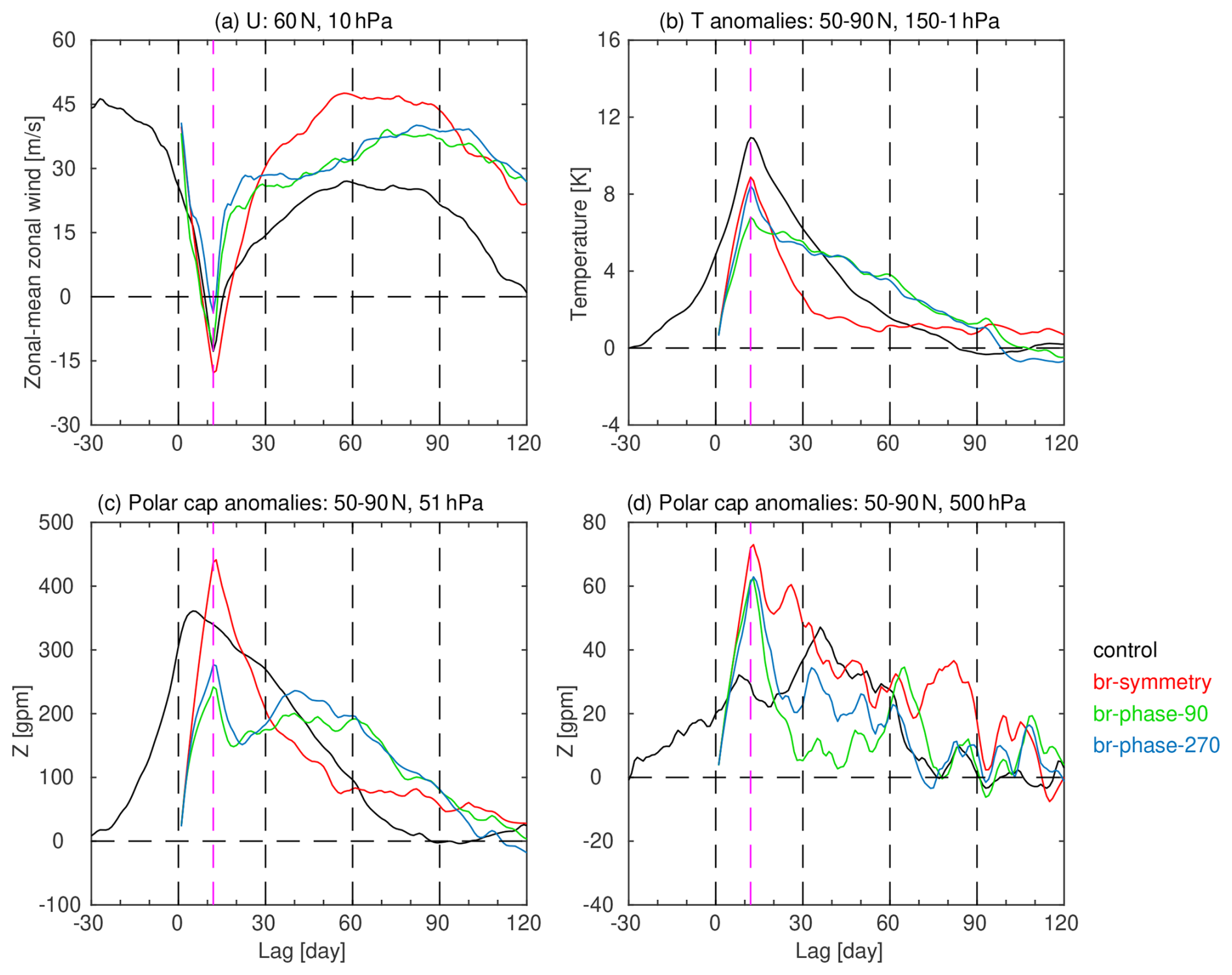
Figure 3 Time series of (a) $\stackrel{\mathrm{‾}}{u}$ (m s⁻¹) at 60° N and 10 hPa, (b) $\stackrel{\mathrm{‾}}{T}$ (K) area-averaged over 50–90° N and pressure-weighted over 150–1 hPa, and polar cap geopotential height anomalies (gpm) area-averaged over 50–90° N at (c) 51 hPa and (d) 500 hPa for the 48 control SSWs (black line) and for various branch ensembles (colored lines) from lag day −30–120. Note that there are 50 ensemble members for each branch ensemble. The vertical magenta dashed line indicates day 12, the day with peak easterlies following the onset of SSW in the control run, and 12 January of every year (the last day with imposed forcing) in the branch ensembles, accompanied by peak easterlies following the onset of forced SSWs too.

Although the accumulated negative forcing is identical across the symmetry, phase-90, and phase-270 ensembles, significant differences are evident in the tropospheric (and also stratospheric) responses, indicating that the longitudinal phase of the imposed wave-1 forcing plays a crucial role in shaping both stratospheric and tropospheric responses (Fig. 2). How do these variations in stratospheric response translate into differences in surface conditions?

4.2 Surface Responses

We begin by analyzing the temporal evolution of 2 m temperature anomalies (Fig. 4). During days 1–12 (while the stratospheric torque is still on), cooling and warming signals emerge but differ widely across the symmetry, phase-90, and phase-270 ensembles (Fig. 4b–d). From day 13 onward, these anomalies intensify, suggesting a continued influence of imposed forcing on surface temperature patterns even after the forcing is turned off. In the control run and symmetry ensemble (Fig. 4a and b), significant cooling occurs over North Eurasia and North America, while warming is observed over subtropical Eurasia and northeast Canada. This temperature response pattern resembles that found in reanalyses (Butler et al., 2017). However, the cooling and warming patterns vary substantially in the phase-90 and phase-270 ensembles. Cooling is most pronounced over Alaska and east Eurasia in the phase-90 ensemble (Fig. 4c), whereas in the phase-270 ensemble (Fig. 4d), it is primarily concentrated over central North America and North Eurasia. The warming patterns also differ between the two asymmetric ensembles. In the phase-90 ensemble (Fig. 4c), warming is primarily located over northwestern Europe, whereas in the phase-270 ensemble (Fig. 4d), it is more prominent over North America and subtropical Eurasia. The persistence and amplification of these anomalies after day 13 (after the forcing is switched off) indicate a causal coupling between the stratosphere and surface, as the stratosphere possesses a longer memory than the troposphere and can exert a prolonged impact on surface conditions (Baldwin et al., 2003). Moreover, the contrasting responses between the phase-90 and phase-270 ensembles underscore the importance of the longitudinal phase of asymmetric forcing in modulating regional surface temperature anomalies. The response in the control run is stronger than that in the branch ensembles in days 1–12, and this likely has two complementary causes: (i) the stratospheric polar vortex is much weaker in the control run than in the branch ensembles in days 1–12 (Fig. 3a and b); (ii) tropospheric precursors of the SSW (specifically a North Pacific low and Ural high; Garfinkel et al., 2010) lead to surface temperature anomalies before the SSW onsets due to a purely tropospheric pathway (Lehtonen and Karpechko, 2016).

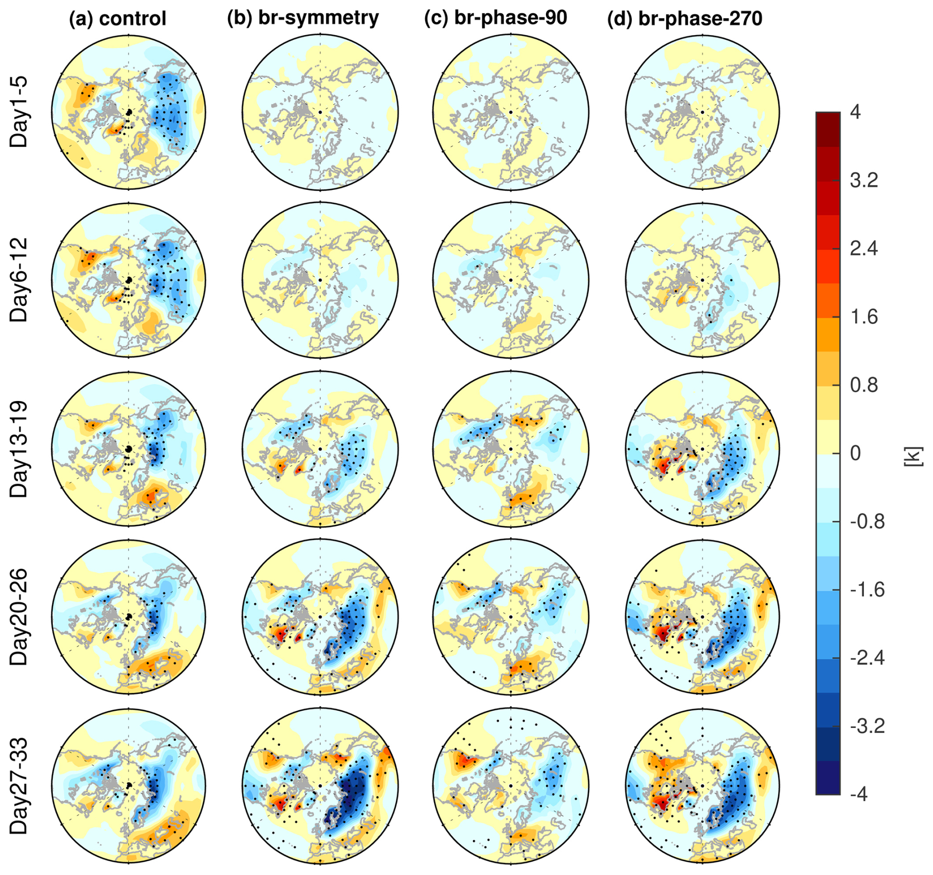
Figure 4 Temporal evolution of 2 m temperature anomalies during days 1–33 for (a) control run, (b) symmetry ensemble, (c) phase-90 ensemble, and (d) phase-270 ensemble. Stippling indicates statistically significant anomalies at the 95 % level based on Student's t test. Recall that the forcing in the branch ensembles is applied only from days 1–12 and is switched off from day 13 onward. Hence, we show the response from days 1–5 and from days 6–12 during the forcing stage, and weeks from day 13 onward during the recovery stage.

Next, the temporal evolution of precipitation anomalies is examined in Fig. 5. During days 1–5, rainfall anomalies begin to emerge, and then these signals intensify significantly, exhibiting notable differences among the symmetry, phase-90, and phase-270 ensembles during days 6–19. Across all experiments, the strongest rainfall anomalies are observed primarily over the North Pacific, extending into North America, and over the North Atlantic, stretching into subtropical Eurasia, which is consistent with the observational results of Butler et al. (2017). However, the distribution of anomalies differs widely between the phase-90 and phase-270 ensembles. Rainfall is particularly enhanced over subtropical Eurasia during days 13–19 in the phase-270 ensemble (Fig. 5d), whereas in the phase-90 ensemble (Fig. 5c), the enhancement of rainfall in Europe is weaker and located further north than for other experiments, while southeastern Europe dries. After peaking during days 13–19, precipitation anomalies weaken rapidly in the phase-90 and phase-270 ensembles, even as the temperature pattern persists in these days (Fig. 4). This evolution suggests that the imposed forcing produces a temporary but pronounced impact on regional precipitation, with rainfall anomalies gradually diminishing as the polar vortex recovers without the influence of momentum torques. By analyzing 24 SSWs that occurred in the 1979–2016 period using the ERA-Interim reanalysis, King et al. (2019) also reported a clear distinction between surface temperature and precipitation patterns: while a cooling signal can persist for up to two months following SSWs, rainfall tends to intensify in the first month and then it is drier in the second month over the Atlantic coast of northern Europe. King et al. (2019) argued that the precipitation patterns align with sea level pressure anomalies before and after the SSW. While the present study will not delve into the mechanisms behind these precipitation anomalies, a detailed investigation will be presented in a subsequent paper.

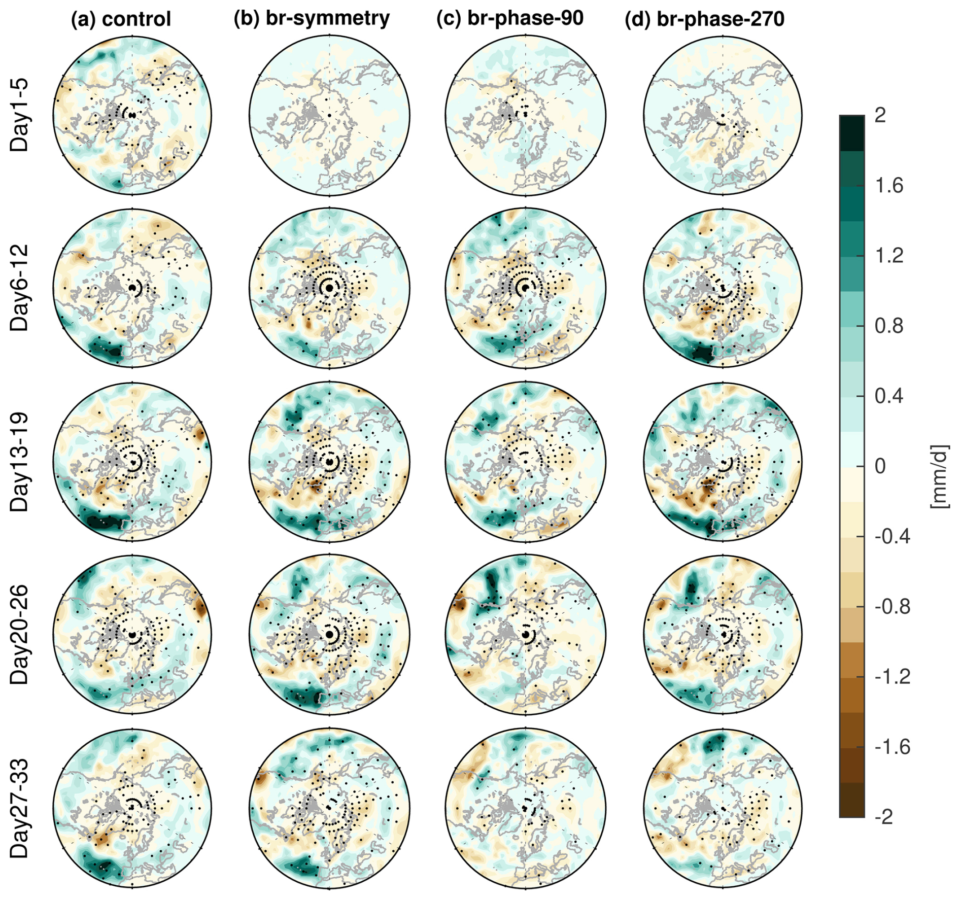
Figure 5 As in Fig. 4 but for precipitation anomalies.

4.3 Wave Reflection and Downward Wave Propagation

Previous studies have argued that wave reflection events during weakened vortex states can lead to surface cooling over North America and North Eurasia (Kretschmer et al., 2018a, b), and we now consider whether such a process is active in these experiments. To begin, we show the longitude-pressure cross section of WAF (F_x, F_z) averaged over days 6–12 in Fig. 6. In all branch experiments, planetary waves propagate upward into the stratosphere and are subsequently reflected back into the troposphere, but the reflections occur over different regions among these experiments. More crucially, the magnitude of the downward reflected waves is much weaker in the symmetry ensemble (Fig. 6b) than in the phase-90 and phase-270 ensembles (Fig. 6c and d), suggesting that the imposed wave forcing can influence the wave reflection events. The shading in Fig. 6 shows the raw geopotential height eddy area-averaged from 55 to 80° N, and there is a clear eastward tilt from 180 to 300° E in the phase-90 ensemble (Fig. 6c) and especially in the phase-270 ensemble (Fig. 6d) with downward-directed arrows from 90 to 270° E, which also indicates the presence of wave reflection events over there (Cohen et al., 2022).

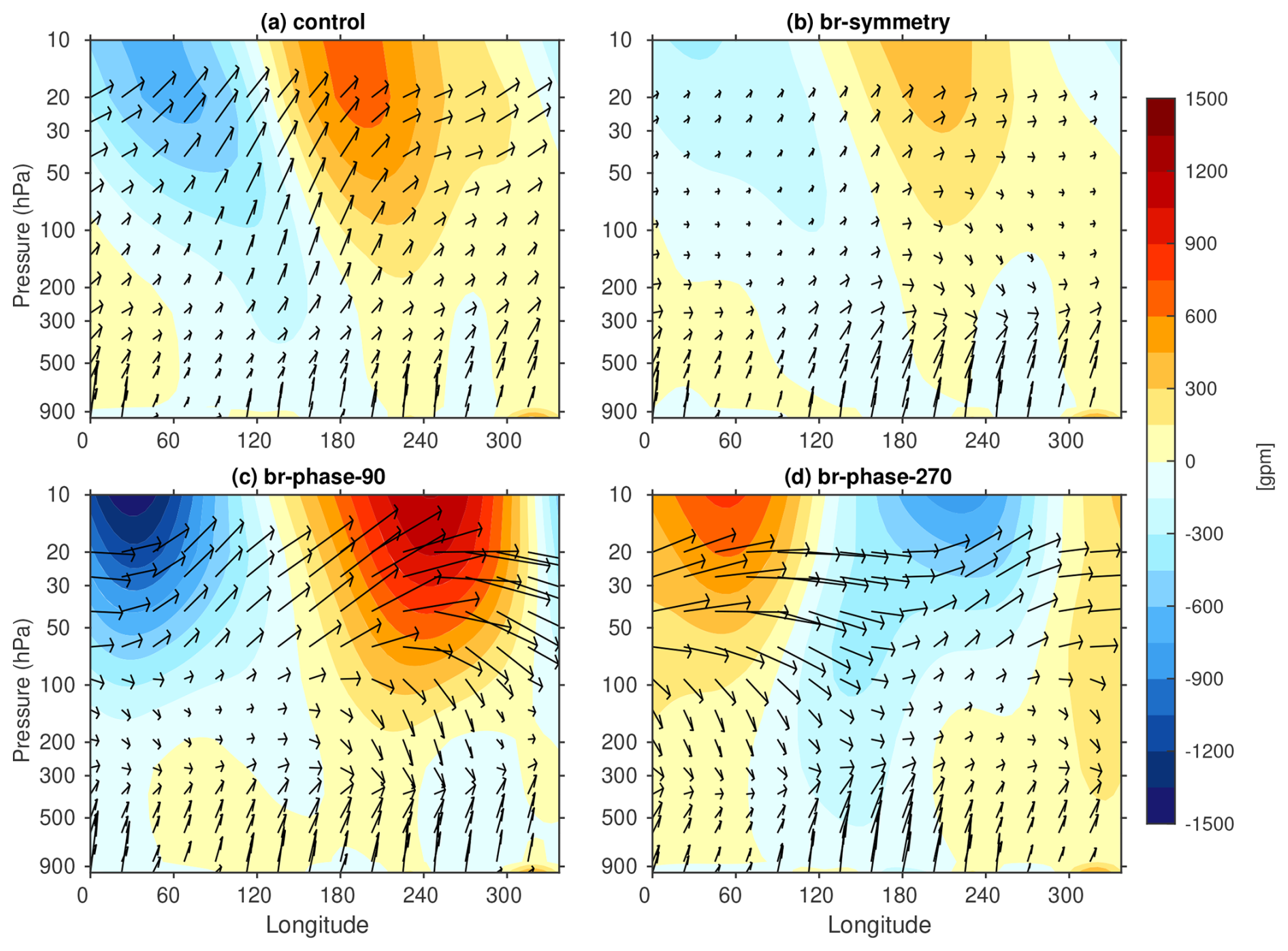
Figure 6 Longitude-pressure cross section of raw F_x and F_z (arrows) and raw geopotential height eddy (shading; deviation from the zonal mean) area averaged between 55–80° N averaged over days 6–12 for (a) control run, (b) symmetry ensemble, (c) phase-90 ensemble, and (d) phase-270 ensemble.

To further illustrate the zonal asymmetries of wave reflection events, Fig. 7 shows the vertical component of WAF (F_z) at 93 hPa during days 1–19. It shows the raw vertical WAF field, not anomalies, and hence negative values of F_z signify a wave reflection event accompanied by downward wave propagation, which can subsequently impact the tropospheric circulation and surface climate (Cohen et al., 2021, 2022; Perlwitz and Harnik, 2003). In the symmetry ensemble, downward wave propagation is mainly located above North America in days 1–12, consistent with climatological downward wave propagation in ERA5 reanalysis data (Messori et al., 2022), but occurs more centrally above the pole in days 13–19 (Fig. 7b). Similarly, the phase-90 ensemble (Fig. 7c) shows strong downward wave propagation localized over North America, but with stronger downward wave propagation than those in the symmetry ensemble (Fig. 7c vs. b), which is then followed by local surface cooling even after the forcing is turned off (Fig. 4c). A similar spatial pattern is also observed in the composite of cluster 4 events in Kretschmer et al. (2018a), which are characterized by raw positive F_z over Eurasia and raw negative F_z over North America. They demonstrated that such events are associated with North American cold spells via reflected upward-propagating waves over eastern Siberia by using causal effect network analysis. In the phase-270 ensemble, downward wave propagation is instead concentrated over North Eurasia, and is immediately followed by pronounced surface cooling over North Eurasia (Fig. 4d). Moreover, observations of cluster 5 in Kretschmer et al. (2018a), characterized by anomalously positive F_z over North America and anomalously negative F_z over Eurasia, show a similar surface temperature response to that in the phase-270 ensemble. However, it is important to understand that cluster 5 in Kretschmer et al. (2018a) does not represent a pure composite of reflection events, as it still displays raw positive F_z over Eurasia despite the anomalously negative F_z.

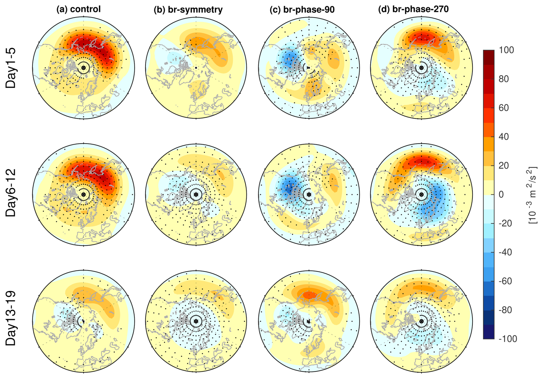
Figure 7 F_z (raw field) at 93 hPa during days 1–19 for (a) control run, (b) symmetry ensemble, (c) phase-90 ensemble, and (d) phase-270 ensemble. Stippling indicates the raw values are statistically significantly different from the climatologies (not shown) at the 95 % level based on Student's t test.

Note that wave reflection is influenced by the imposed momentum torque during the forcing stage from days 1–12. Even though the forcing is switched off during days 13–19, the surface temperature impacts appear strongest only then. This indicates that feedbacks are kicked off and influence the wave reflection even after the forcing is switched off. These results suggest that the opposite phase of wave-1 forcing critically influences the positioning of the wave reflection event and, consequently, modulates regional surface temperature anomalies. A key question arises: through which dynamical pathway do these SSWs and concurrent downward wave propagation events ultimately affect surface conditions?

4.4 Downward Coupling

Here, we delve deeper into the underlying mechanisms driving the surface cooling and warming due to SSWs and downward wave propagation events. A key driver is the anomalous acceleration of the BDC, which plays a crucial role in stratosphere-troposphere coupling with downward motion over the pole, accompanied by enhanced poleward motion in the stratosphere. This acceleration of the BDC is due to the “Eliassen adjustment” which brings high angular momentum air from low latitudes to counteract the weakening of westerlies in high latitudes (Eliassen, 1951), and compensating equatorward motion in the troposphere (Baldwin et al., 2021; White et al., 2022). Specifically, White et al. (2022) found that the subsidence in the troposphere over the pole and the subsequent near-surface northerly winds help induce the near-surface jet response in the first few days and weeks after the SSW onset before synoptic eddy feedbacks kick in.

To examine this effect, we calculate the mass streamfunction by pressure-integrating the divergent component of meridional wind over 34–10 hPa in Fig. 8, and over 700–321 hPa in Fig. 9 (see Sect. 3.1). In the stratosphere (Fig. 8), significant poleward motion is observed across all experiments. Under the influence of symmetric forcing, this poleward motion is broadly distributed over the circumpolar region in the symmetry ensemble (Fig. 8b). In contrast, the phase-90 ensemble exhibits poleward motion primarily over the eastern hemisphere during days 1–5 (Fig. 8c), whereas in the phase-270 ensemble, it shifts to the western hemisphere (Fig. 8d). This contrasting circulation pattern underscores how wave-1 forcing with opposite phase induces distinct and spatially opposing effects in the stratosphere.

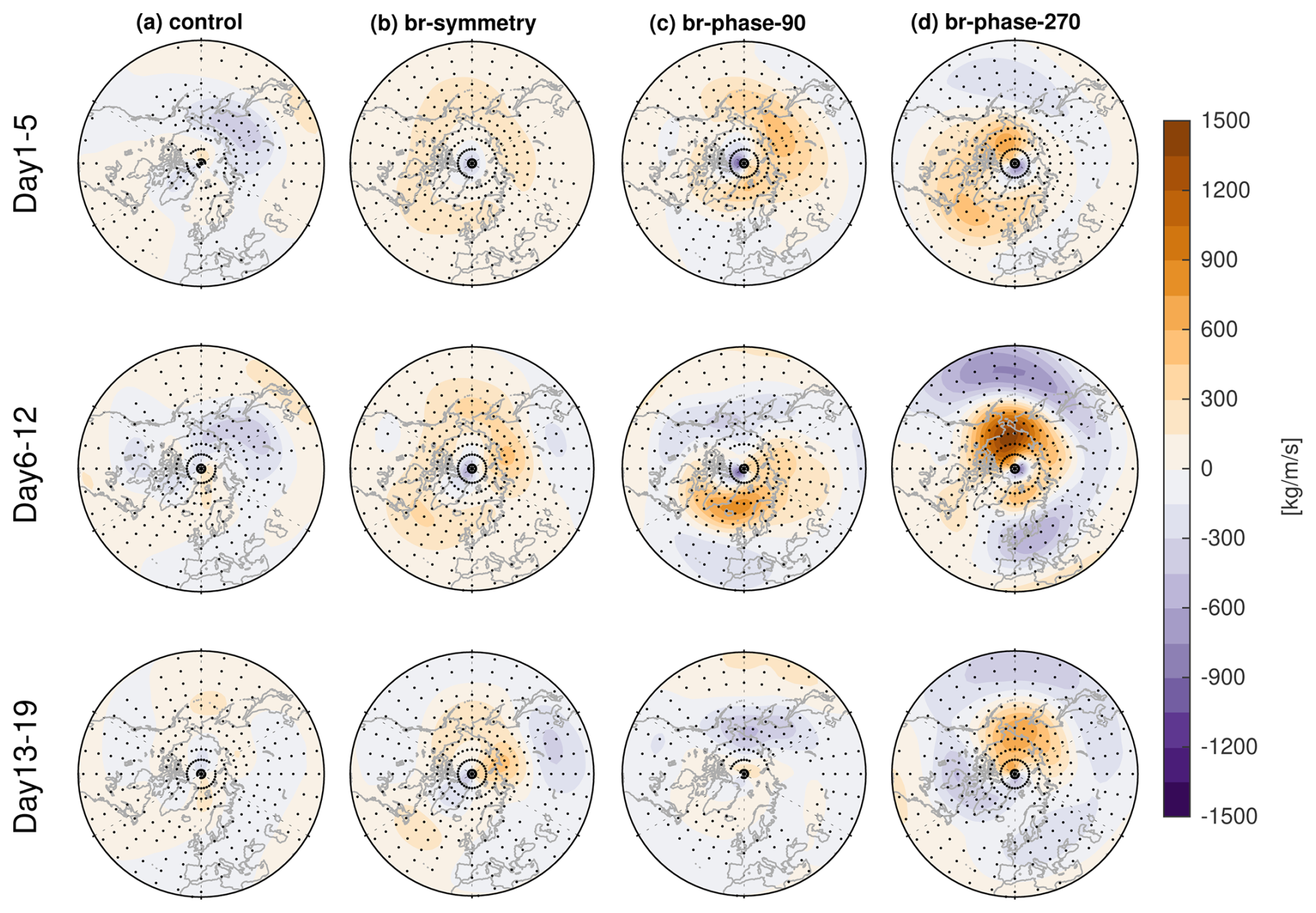
Figure 8 Mass streamfunction (derived from divergent component of meridional wind) anomalies pressure-weighted over 34–10 hPa during days 1–19 for (a) control run, (b) symmetry ensemble, (c) phase-90 ensemble, and (d) phase-270 ensemble. Stippling indicates statistically significant anomalies at the 95 % level based on Student's t test. Based on the conventions in Sect. 3, positive anomalies indicate poleward meridional flow, and negative anomalies indicate equatorward flow.

A similar but opposite-signed circulation pattern emerges in the free troposphere (Fig. 9), where equatorward motion is significantly intensified across all experiments. Notably, in the phase-90 and phase-270 ensembles (Fig. 9c and d), the tropospheric circulation exhibits a zonal dipole structure that is spatially aligned with the corresponding stratospheric circulation but with an opposite sign. Namely, tropospheric northerlies are strongest over Alaska in the phase-270 ensemble and over Eurasia in the phase-90 ensemble even after the forcing has ended (Fig. 9c and d). This correspondence between the mass streamfunction in the stratosphere and in the troposphere indicates that the mechanism of White et al. (2022) for zonally symmetric SSWs also manifests in response to the zonally asymmetric torques applied here: the troposphere dynamically adjusts to the stratospheric torque, with the biggest impact in the same sector as the applied stratospheric torque.

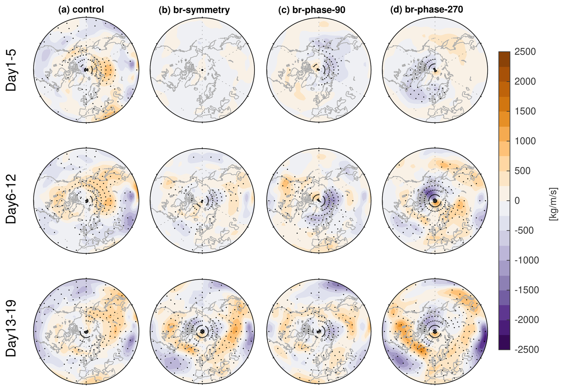
Figure 9 As in Fig. 8 but over 700–321 hPa.

This divergent meridional circulation diagnosed by the mass streamfunction can subsequently induce changes in zonal wind via Coriolis torques (as in White et al., 2022). We demonstrate this with the zonal wind anomalies at 321 hPa in Fig. 10. In all experiments, zonal winds substantially weaken over the circumpolar regions, leading to an equatorward shift of the tropospheric jet, consistent with observations during real SSWs (Baldwin et al., 2021). In the branch ensembles (Fig. 10b–d), the strongest negative zonal wind anomalies coincide well with the imposed negative forcings in the stratosphere, exhibiting weaker amplitude than those at 10 hPa but stronger than those at 850 hPa (Fig. 1b and c). This pattern indicates that the tropospheric jet responds to the imposed stratospheric wave forcings in days 6–12, and, in turn, the jet changes lead to the rest of the tropospheric response. However, the equatorward jet shift, characterized by a pronounced meridional dipole (Fig. 10c and d), primarily emerges over the North Pacific in the phase-90 ensemble, whereas it predominantly occurs over the North Atlantic and extends into subtropical Eurasia in the phase-270 ensemble. This jet displacement pattern leads to more intensified precipitation anomalies over the corresponding regions in the phase-90 and phase-270 ensembles (Fig. 5c and d). Moreover, during the forcing stage (days 6–12), the tropospheric jet shifts in the opposite direction to the displacement of the center of anomalous poleward circulation in the forced stratosphere between the phase-90 and phase-270 ensembles (Fig. 8c and d; middle row). Although the stratospheric streamfunction weakens after the wave forcing is switched off (days 13–19; Fig. 8c and d; bottom row), the tropospheric jet and associated tropospheric streamfunction instead intensify (Fig. 9c and d; bottom row), suggesting that tropospheric eddy feedbacks kick in after the stratospheric forcing ceases to maintain the jet shift.

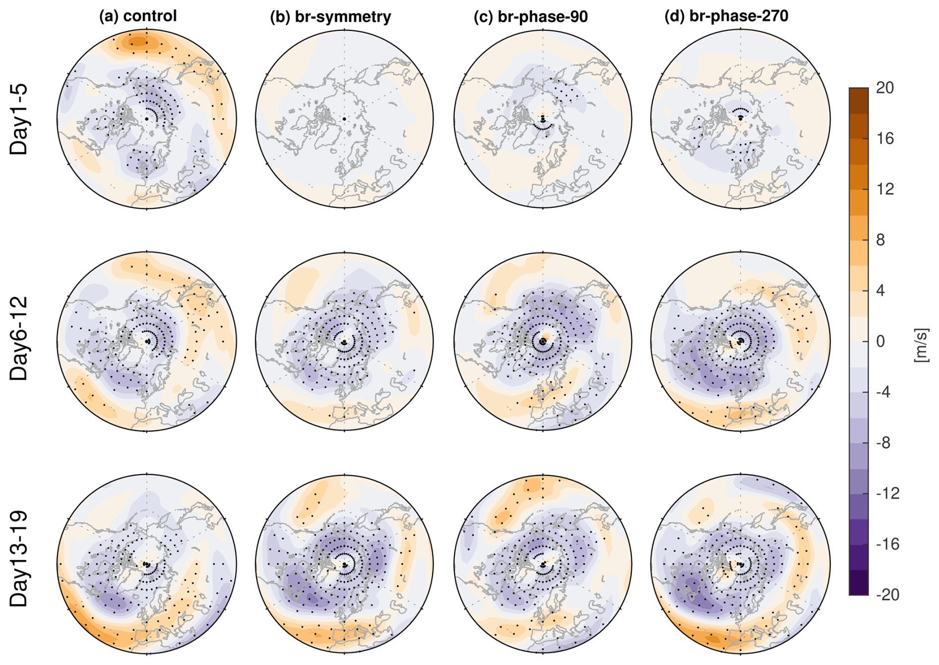
Figure 10 Zonal wind anomalies at 321 hPa during days 1–19 for (a) control run, (b) symmetry ensemble, (c) phase-90 ensemble, and (d) phase-270 ensemble. Stippling indicates statistically significant anomalies at the 95 % level based on Student's t test.

Next, to investigate the role of downward coupling in shaping regional surface temperature anomalies, we show the mass streamfunction pressure-integrated over 970–850 hPa in the lower troposphere in Fig. 11. Across all experiments, significant equatorward motion is broadly observed around the pole, while poleward motion primarily occurs over subtropical Eurasia. These circulation patterns peak after the forcing switches off (in contrast to the stratospheric poleward motion, which peaks during the forcing period – Fig. 8), which is the same as the tendency of surface temperature anomalies (Fig. 4) and variations of the tropospheric jet (Fig. 10). These results highlight that the imposed forcing significantly influences the surface temperature during the forcing stage (days 1–12), whereas the tropospheric jet response plays a key role in amplifying the anomalies once the forcing is removed. In particular, equatorward motion facilitates the southward transport of colder air masses from the pole to the subtropics, thus inducing pronounced cooling over Alaska and eastern Eurasia in the phase-90 ensemble (Fig. 4c) and over northern and western Eurasia in the phase-270 ensemble (Fig. 4d). Conversely, poleward motion advects warmer air masses from lower latitudes toward higher latitudes, but is much more pronounced over Eurasia in the phase-270 ensemble than in the phase-90 ensemble, consistent with the broader and more robust warming over mid-latitude Eurasia in the phase-270 ensemble than in the phase-90 ensemble (Fig. 4c and d). Furthermore, the spatially limited poleward flow over northwestern Europe in the phase-90 ensemble is consistent with the warming signal over northwestern Europe evident only in that ensemble (Fig. 4c). Quantifying the importance of this mechanism as compared to the advection of temperature by the anomalous rotational component of wind is left for future work.

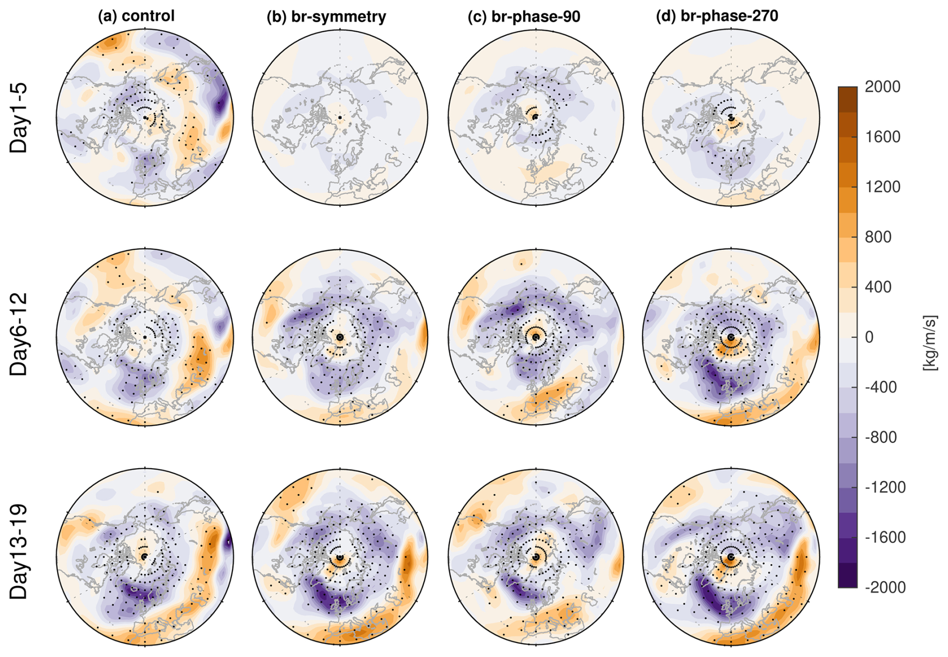
Figure 11 As in Fig. 8 but over 970–850 hPa.

This dynamical interaction between equatorward and poleward motions underscores the important role of the lower tropospheric meridional circulation in modulating regional surface temperature patterns. While this mechanism is not the sole driver accounting for cooling and warming patterns following SSWs and concurrent wave reflection events, it represents a critical pathway through which stratospheric perturbations propagate downward and ultimately influence surface conditions. Overall, this study highlights the crucial role of the mass streamfunction by the divergent component of meridional wind in facilitating stratosphere-troposphere coupling during SSWs and concurrent wave reflection events, ultimately leading to distinct surface cooling and warming patterns.

5 Discussion and Conclusions

A better understanding of the surface response to zonal asymmetries of the polar vortex, and specifically of wave reflection during weak vortex states, is important. While previous work using observational data has found evidence that the zonal structure of the vortex anomaly and downward wave propagation matters for the surface impact, it is difficult to isolate the causality using observational data as typically the anomalous vortex state was preceded by a burst of wave activity in the troposphere, and it is not clear how to separate the long-term effects of this initial wave activity from the subsequent stratospheric and tropospheric response.

For example, while both displacement- and split-SSWs affect surface temperatures with potential differences in the spatial pattern and magnitude (Hall et al., 2021; Mitchell et al., 2013), these different SSW morphologies are preceded by qualitatively different initial tropospheric wave fluxes: displacement-SSWs are primarily driven by wave-1 forcing, whereas split-SSWs are influenced by a combination of wave-1 and wave-2 forcings (Bancalá et al., 2012; Cohen and Jones, 2011; White et al., 2019). In addition to SSW events, wave reflection events can also significantly impact the surface weather, often leading to extreme cooling over North America (Cohen et al., 2021, 2022; Matthias and Kretschmer, 2020). But wave reflection events are also typically preceded by a burst of wave activity over Siberia, and it is not trivial to isolate the importance of the stratospheric reflection from the tropospheric wave activity over Siberia for the subsequent North America response. While there are advanced techniques based on causal effect networks or Granger/Pearl causality that have been applied (Kretschmer et al., 2018a, b), these techniques ultimately do not allow for a clear mechanistic understanding. Further, the dynamical mechanism(s) accounting for the varying surface responses to different types of SSWs and associated wave reflection events remain insufficiently understood.

To investigate the role of zonal asymmetries of the polar vortex and the wave reflection phenomenon during SSW events, we extend the approach of White et al. (2022) by adding momentum torques with a strong zonally asymmetric component in the stratosphere of the MiMA model (Garfinkel et al., 2020a; Jucker and Gerber, 2017). Taking every midnight on 1 January from the CTRL run as an initial condition, we branch off and impose a momentum torque with various longitudinal phases. In the present study, we focus on two representative perturbation experiments, phase-90 ensemble (k=1, Θ_A = 4, λ₀ = 90°) and phase-270 ensemble (k=1, Θ_A = 4, λ₀ = 270°). More experiments will be analyzed in a subsequent paper. These branch ensembles are compared to 48 spontaneously occurring SSWs in control runs.

The zonally opposite pattern of wave-1 forcing leads to contrasting influences in the stratosphere and troposphere. During the forcing stage, the zonal mean zonal wind at 60° N and 10 hPa suddenly transitions from westerlies to easterlies under the impact of the easterly torque (Fig. 3a). Concurrently, the polar cap becomes warmer and exhibits a higher geopotential height (Fig. 3b–d), as the enhanced downwelling in the BDC leads to more adiabatic heating (Baldwin et al., 2021; Garfinkel et al., 2010). In the phase-90 and phase-270 experiments, stratospheric zonal wind anomalies peak in opposite hemispheres, and this difference in the stratosphere is mirrored by a qualitatively different impact in the troposphere (Fig. 1). Furthermore, the polar vortex shifts away from the pole, but in opposite directions at 10 hPa during days 6–12 (Fig. 2c and d) due to the opposite phasing of the wave-1 component of the forcing. The tropospheric geopotential height anomalies also exhibit significant displacements from the pole, with the direction of the shift mirroring that in the stratosphere and opposite between the different experiments. Overall, the opposite phase of wave-1 forcing induces markedly different impacts on the zonal wind, temperature, and geopotential height fields throughout the stratosphere and troposphere by downward dynamical coupling.

Furthermore, this downward coupling also influences the 2 m temperature and precipitation patterns. Signals of cooling, warming, and enhanced rainfall appear while the forcing is still on, though their spatial distributions differ among these experiments. The cooling and warming signals intensify well after the stratospheric forcing is turned off (Fig. 4), while rainfall anomalies peak immediately after the forcing is turned off (in days 13–19) before subsequently weakening (Fig. 5). In the phase-90 ensemble, cooling is most pronounced over Alaska and eastern Eurasia (Fig. 4c), with enhanced rainfall concentrated over the North Pacific and North Atlantic, extending to northwestern Europe (Fig. 5c). However, the phase-270 ensemble exhibits significant cooling over central North America and North Eurasia (Fig. 4d), with intensified rainfall over the North Pacific and North Atlantic, stretching into subtropical Eurasia (Fig. 5d). These surface temperature anomalies in phase-90 and phase-270 ensembles are consistent with the observed surface temperature anomalies in clusters 4 and 5 (Kretschmer et al., 2018a).

The imposed stratospheric forcing results in wave reflection in the lower stratosphere. Downward wave propagation occurs over North America in the phase-90 ensemble (Fig. 7c), consistent with that in cluster 4 of Kretschmer et al. (2018a). However, it is concentrated over North Eurasia in the phase-270 ensemble (Fig. 7d), consistent with the anomalous F_z pattern in cluster 5 observed by Kretschmer et al. (2018a). These results indicate that the opposite phase of wave-1 forcing modulates the SSWs and concurrent wave reflection events differently, leading to distinct impacts on the surface temperature and precipitation patterns. Note that these surface temperature and precipitation patterns arise from the joint impact of SSWs and concurrently occurring wave reflection events.

We elucidate the pathway of stratosphere-troposphere coupling associated with SSWs and wave reflection events by analyzing the mass streamfunction of the divergent component of the meridional wind. In all experiments, significant poleward motion occurs in the stratosphere (Fig. 8), while pronounced equatorward motion emerges in the troposphere (Fig. 9). However, the meridional mass streamfunction exhibits opposite zonal dipole patterns between the phase-90 and phase-270 ensembles. In the stratosphere while the torque is being applied, poleward motion is predominantly located over the eastern hemisphere in the phase-90 ensemble (Fig. 8c), whereas it is centered over the western hemisphere in the phase-270 ensemble (Fig. 8d). This zonal asymmetry in the stratospheric meridional circulation is mirrored in the free troposphere, indicating a robust downward coupling between the stratosphere and troposphere. The tropospheric jet also responds to the forced stratospheric meridional circulation (Fig. 10c and d), but shifts in the opposite direction to the center of the anomalous poleward circulation (Fig. 8c and d), thereby bridging the downward coupling between the forced stratosphere and the free troposphere. It further amplifies the tropospheric meridional circulation (Fig. 9c and d), precipitation anomalies (Fig. 5c and d), and surface temperature patterns (Fig. 4c and d) in days 13–19 even when the forcing is switched off. In the lower troposphere (Fig. 11), equatorward flow transports colder air from higher to lower latitudes, contributing to surface cooling over Alaska and eastern Eurasia in the phase-90 ensemble (Fig. 4c), and over North Eurasia in the phase-270 ensemble (Fig. 4d). Conversely, poleward flow conveys warmer air from subtropical regions toward the poles, resulting in surface warming over northwestern Europe in the phase-90 ensemble (Fig. 4c) and over subtropical Eurasia in the phase-270 ensemble (Fig. 4d).

Overall, the results of this study bolster the conclusions of previous reanalysis-based studies, which link surface cooling and warming patterns to stratospheric wave reflection (Cohen et al., 2021, 2022; Kretschmer et al., 2018a). Namely, for the first time to the best of our knowledge, we have demonstrated that an imposed stratospheric forcing which generates SSWs and concurrent downward wave propagation events can causally produce the surface impacts identified in previous observational work. Moreover, our work highlights that the direction in which the polar vortex is displaced during an SSW displacement event is of crucial importance for the zonal asymmetries of downward wave propagation events and, consequently, the distinct surface responses. Ongoing work will explore other longitudinal phases for a wave-1 forcing and also wave-2 forcings, and also better quantify the relative importance of meridional divergent flow vs. rotational flow in modulating surface temperature anomalies.