The role of the stratospheric state in upward wave flux prior to Sudden Stratospheric Warmings: a SNAPSI analysis

Several studies highlight the relevance of considering polar winter stratospheric information such as the occurrence of Sudden Stratospheric Warmings (SSWs) for skillful Subseasonal to Seasonal (S2S) surface climate predictions. However, current S2S forecast systems can only predict these events about two weeks in advance. A potential way of increasing their predictability is to improve the models' representation of the triggering mechanisms of SSWs. Traditional theories indicate that SSWs follow sustained wave dissipation in the stratosphere, but the relative role of tropospheric versus stratospheric conditions in the enhancement of stratospheric wave activity remains unclear.

This study aims to quantify the role of the stratospheric state in wave activity preceding SSWs by analyzing three recent SSWs: the boreal SSWs of 2018 and 2019 and the austral minor SSW of 2019, using specific sets of S2S experiments. These ensembles follow the SNAPSI (Stratospheric Nudging And Predictable Surface Impacts) guidelines and include free-evolving atmospheric runs and nudged simulations, where the zonally-symmetric stratospheric state is nudged to either observations of a certain SSW or a climatological state. Our results show that the models struggle to capture the strong enhancement of wave activity preceding the 2018 SSW, limiting predictability beyond 10 d. In contrast, both SSWs of 2019 are better predicted, consistent with a more accurate simulation of the wave activity. Nudging the zonal mean stratospheric state does not drastically influence the upward wave activity flux or tropospheric circulation anomalies prior to these SSWs, but it has some impact on the stratospheric wave activity, although this modulation depends on the event characteristics. The boreal 2019 SSW appears to be primarily driven by tropospheric processes. In contrast, stratospheric contributions may have also played an important role in triggering the boreal 2018 SSW and the austral 2019 SSW. Understanding these variations is key to improving SSW predictability in S2S models.

1 Introduction

Sudden stratospheric warmings (SSWs) are the most dramatic example of wintertime polar stratospheric dynamical variability. They are characterized by a rapid increase of polar temperatures and a complete reversal of the climatological westerly winds in the middle stratosphere (Baldwin et al., 2021). The associated effects of these phenomena span beyond the stratosphere. For instance, in the troposphere the SSW signal projects onto a negative phase of the Annular Mode that can persist for several weeks up to two months (Baldwin and Dunkerton, 2001).

Given the persistent influence of SSWs on tropospheric weather, incorporating stratospheric information into subseasonal to seasonal (S2S) forecast systems has proven beneficial for increasing the skill of S2S predictions of surface climate (e. g., Sigmond et al., 2013; Domeisen et al., 2020b). However, current S2S forecast systems can predict SSWs only about two weeks before they occur (Domeisen et al., 2020a; Chwat et al., 2022). Thus, improving the predictability of SSWs within these models is crucial for obtaining better wintertime S2S surface weather forecasts. One potential strategy to achieve this is by improving the models' representation of SSW triggering mechanisms, which, in turn, requires a deeper understanding.

Traditional theories indicate that SSWs are preceded by sustained wave dissipation in the stratosphere, primarily driven by wave amplification and nonlinear wave breaking in that layer (Baldwin et al., 2021 and references herein). The main waves involved in this process correspond to ultra-long planetary (e.g. of wavenumbers 1 and 2) waves that are primarily generated in the troposphere by topography and thermal land-sea contrasts (Garfinkel et al., 2010). Thus, the tropospheric state and its effects on planetary-scale waves play a key role in the wave amplification. However, the stratosphere also exerts some control over the upward-propagating wave activity. For instance, Rossby waves can only propagate in westerly winds, meaning that tropospheric waves only reach the stratosphere from autumn to spring (Charney and Drazin, 1961). The interactions between waves and the stratospheric mean flow also influence wave amplification. As waves dissipate, they decelerate the westerly mean flow, allowing a stronger upward propagation of wave activity if there is no wind reversal (Holton and Mass, 1976). Thus, the exact cause of the wave amplification leading to the occurrence of an SSW, and specifically the relative roles of the stratospheric and tropospheric states, are still under debate (Butchart, 2022).

Some authors emphasize the importance of enhanced and persistent tropospheric wave forcing as a key factor in initiating an SSW (e.g.: Matsuno, 1971). In this scenario, the development of an SSW then takes some time, since the wave activity builds up over time starting from the tropospheric source and propagating upward into the stratosphere (Cohen and Jones, 2011; Sjoberg and Birner, 2012; Schwartz and Garfinkel, 2017). In contrast, other studies have provided evidence of wave amplification occurring within the stratosphere without a corresponding enhancement of wave activity in the troposphere (e.g., Jucker, 2016; Birner and Albers, 2017; de la Cámara et al., 2019). This may result from two distinct mechanisms: the first is a “valve” effect of the lower stratospheric basic flow, modulating and/or channeling the wave activity flux that enters into the stratosphere (e.g., Chen and Robinson, 1992; Scott and Polvani, 2004, 2006; Hitchcock and Haynes, 2016); the second is through resonant wave growth excited by the stratospheric flow configuration (e.g., Clark, 1974; Plumb, 1981; Smith, 1989; Matthewman and Esler, 2011; Esler and Matthewman, 2011; Albers and Birner, 2014). Regardless of the mechanism at work, the evolution of the stratosphere towards an SSW-favorable state is generally known as “preconditioning” (McIntyre, 1982; Lawrence and Manney, 2020) and may involve changes in the stratospheric basic state not directly linked to the polar vortex.

Observational evidence supports both the tropospheric and stratospheric roles in triggering SSWs and suggests that the mechanism at play may depend on the type of SSW. Whereas anomalous tropospheric wave activity tends to precede wavenumber-1 (WN1) events (Birner and Albers, 2017), wave resonant processes in the stratosphere are more likely to be involved in triggering wavenumber-2 (WN2) SSWs (Albers and Birner, 2014). In any case, the main difficulty of analyzing the different triggering mechanisms in observations or comprehensive models lies in the inherent nonlinear wave-mean flow interactions involved, which hinders efforts to distinguish cause from effect (e.g., Sjoberg and Birner, 2014; de la Cámara et al., 2017). Clarifying these dynamics is crucial for improving SSW predictability.

While these dynamics can be clarified using idealized models (e.g., Gerber and Polvani, 2009; Hitchcock and Haynes, 2016; Dunn-Sigouin and Shaw, 2020), these models necessarily simplify key processes such as radiative relaxation in the stratosphere. An alternate approach is to nudge the atmospheric state in a certain region or layer in complex models, which may help to disentangle the role of the troposphere and stratosphere in triggering SSWs. Indeed, this technique has been successfully applied in climate models (de la Cámara et al., 2017) or even in S2S models (e.g. Kautz et al., 2020), although for a different purpose in the latter case. Most of these studies have used only one model, but S2S models have biases in the stratospheric state and wave activity (Lawrence et al., 2022; Garfinkel et al., 2025). Thus, the results derived from a single model study can be influenced by these biases and a multimodel approach would be more appropriate.

In this study, we aim to investigate the stratospheric role in the amplification and propagation of upward wave activity during SSWs. The use of a set of S2S experiments of the Stratospheric Nudging And Predictable Surface Impacts (SNAPSI) project (Hitchcock et al., 2022) provides a unique opportunity to achieve this goal. The SNAPSI experiments are performed with several S2S models following the same requirements. They are designed to isolate the effects of the zonal mean stratospheric state (through nudging) on the rest of the atmosphere and in particular, on the troposphere during three SSWs: the boreal SSWs of 12 February 2018 and 2 January 2019 and the austral minor SSW of September 2019. These events were very different in many regards. In terms of surface impacts, the SSW of 2018 (SSW2018) and the austral SSW (SSW2019 SH) led to numerous extreme surface events (Ayarzagüena et al., 2018; Kautz et al., 2020; Lim et al., 2021), while the influence on surface weather of the boreal SSW of 2019 (SSW2019) was weak (Butler et al., 2020). The two SSWs of 2019 were predictable by S2S systems at longer lead times than the 2018 event (Butler et al., 2020; Rao et al., 2020a, b). The dynamics that preceded the three events also differed remarkably: The SSW2018 was preceded by a rapid amplification of WN2 wave activity, whereas the other two events were mainly associated with strong WN1 wave activity (Karpechko et al., 2018; Butler et al., 2020; Lim et al., 2021).

Previous studies have shown that WN2 SSWs are more difficult to forecast than WN1 events (Taguchi, 2018; Domeisen et al., 2020a; Chwat et al., 2022), but the underlying physical reasons remain unclear. While Taguchi (2018) performed a systematic multimodel analysis of tropospheric precursors and wave activity preceding SSWs, SNAPSI will allow us to make a step forward on this topic by investigating and isolating the influence of the stratospheric state on these triggering mechanisms depending on the type of event. In addition, SNAPSI will also contrast the ability of S2S forecast systems to reproduce each of the three events. In particular, we first assess the ability of different S2S forecast systems to reproduce the stratospheric wave amplification and tropospheric wave structures preceding the SSWs in Sect. 3. Secondly, we investigate the influence of the stratospheric state on the triggering mechanisms of the three SSWs in Sect. 4. Given the models' low skill in predicting the SSW2018 and the associated wave activity, we perform a detailed analysis of the upward wave propagation prior to this event in Sect. 5.

2 Data and methodology

2.1 SNAPSI experiments

As previously mentioned, we use the set of ensemble SNAPSI experiments of eight S2S forecast systems (Table 1). These ensembles include free-evolving atmospheric runs (FREE experiment) and nudged simulations where the zonally-symmetric stratospheric state is nudged globally to either observations of a specific SSW (NUDGED) or a time-evolving climatology (CONTROL) (Hitchcock et al., 2022). The stratospheric states in these nudged ensembles are derived from 6-hourly data taken from ERA5 reanalysis at model levels (Hersbach et al., 2020). For the CONTROL ensemble, the daily climatological state is calculated as the average of ERA5 data from 1 July 1979 to 30 June 2019. The zonally symmetric states used for NUDGED and CONTROL correspond to instantaneous zonal-mean temperature and zonal wind from ERA5 at 6 h intervals (Hitchcock et al., 2022). The nudging consists of a relaxation tendency towards the zonally symmetric reference state to which the flow is constrained as follows: $-{\mathit{\tau }}^{-\mathrm{1}}(X-X_t)$, where X is the field to be nudged and X_t corresponds to the reference stratospheric state to which the field is constrained. The nudging is applied gradually in the vertical starting at 90 hPa and reaching the full strength at 50 hPa. This is expressed by modifying the timescale of the relaxation with height as: $\mathit{\tau }=\mathrm{6}\mathrm{h}\cdot {\left(\frac{p_b-p}{p_b-p_t}\right)}^{\mathrm{3}}$, where p_b=90 hPa and p_t=50 hPa. The choice of these vertical levels is made to avoid a direct impact on the troposphere following the recommendations of previous research (Hitchcock and Haynes, 2016). The stratospheric nudging is imposed at all latitudes and longitudes equally, so that the zonally asymmetric part of the flow and thus, the wave field are not affected. This latter point is particularly important for the purpose of the present study, focused on the wave activity flux. In all cases, as mentioned in Hitchcock et al. (2022), wave activity fields in the sensitivity experiments are comparable to the corresponding ones in the FREE experiments despite prescribing the zonal mean stratospheric state. The nudging can indeed interfere with the interaction between the waves and the mean flow which can then impact the wave structures themselves, but Hitchcock et al. (2022) found this to only have significant impacts on wave amplitudes in the upper stratosphere as a result of waves propagating to higher levels in the absence of their ability to decelerate the mean flow lower down.

Table 1 List of models included in the analysis indicating their resolution and key reference(s).

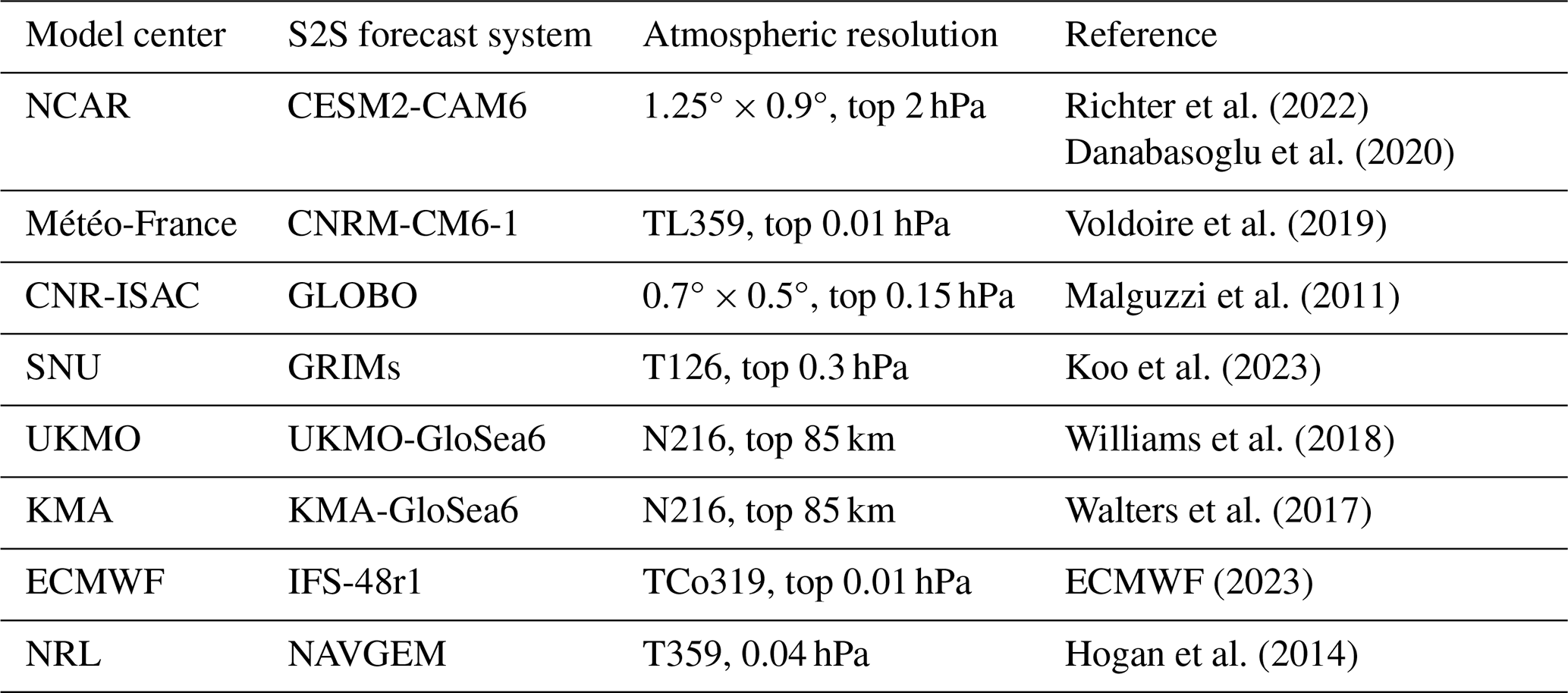
Each forecast integration spans 45 d, with ensemble sizes of 50 members, except for the NAVGEM model that includes 80 members. Furthermore, each experiment is initialized on two distinct dates for each SSW event: one prior to the onset of the event and another approximately three weeks before the associated surface extreme events. Since our focus here is on the mechanisms that trigger SSWs, we use the first initialization dates with a similar forecast lead time with respect to the SSW: 25 January 2018 (18 d before the event), 13 December 2018 (20 d before the event), and 29 August 2019 (17 d prior to the SSW). For further details, please refer to Hitchcock et al. (2022).

Throughout the study, results derived from SNAPSI experiments are compared with those obtained with ERA5. Anomalies in reanalysis and models are computed with respect to ERA5 climatology over the period 1979/80–2018/19.

2.2 Methods

We describe here the metrics and techniques used to achieve our goals. Since our focus is on the mechanisms that trigger SSWs, these diagnostics emphasize event identification and quantification of wave activity fluxes.

2.2.1 SSW identification

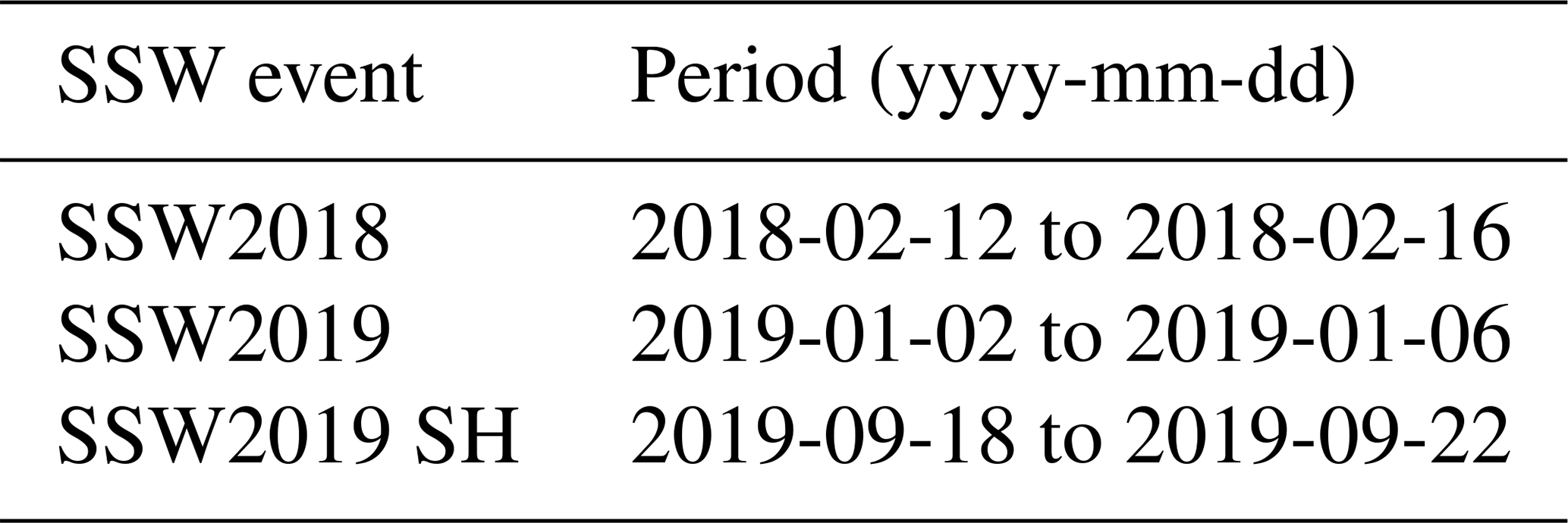
SSWs in the Northern Hemisphere (NH) are identified by the reversal of the westerly zonal-mean zonal wind at 60° N and 10 hPa to easterly (Charlton and Polvani, 2007). Once an event is detected in a given realization, the search for additional SSWs within the same realization is stopped. For the Southern Hemisphere (SH) case, the observed SSW2019 SH was classified as a minor warming with a strong deceleration of the wind but without a full reversal. Thus, the SH events are identified when the zonal-mean zonal wind at 60° S and 10 hPa weakens below 20 m s⁻¹ (as in Rao et al., 2020a).

2.2.2 Diagnostics of wave activity

Several diagnostics are used to analyze wave activity, particularly upward wave activity flux. These diagnostics include the Eliassen-Palm flux and the zonal-mean meridional eddy heat flux averaged over 45 −75° (HF).

The Eliassen-Palm flux (EP flux, F) (Eq. 1) represents the flux of wave activity, providing insights into the dynamics of wave-mean flow interactions (Edmon et al., 1980).

$$\begin{array}{}\text{(1)}& \mathit{F}=\left(F_{\mathit{\varphi }},F_z\right)\end{array}$$

where the two F components are defined as follows (Andrews et al., 1987):

$$\begin{array}{}\text{(1.1)}& {\displaystyle }{F}_{\mathit{\varphi }}=\mathit{\rho }a\cos \mathit{\varphi }\left[-\stackrel{\mathrm{‾}}{u^{\prime }{v}^{\prime }}+{\displaystyle \frac{\partial \stackrel{\mathrm{‾}}{u}}{\partial z}}{\displaystyle \frac{\stackrel{\mathrm{‾}}{v^{\prime }{\mathit{\theta }}^{\prime }}}{\frac{\partial \stackrel{\mathrm{‾}}{\mathit{\theta }}}{\partial z}}}\right]\text{(1.2)}& {\displaystyle }{F}_z=\mathit{\rho }a\cos \mathit{\varphi }\left[\left(f-{\displaystyle \frac{\mathrm{1}}{a\cos \mathit{\varphi }}}{\displaystyle \frac{\partial \left(\stackrel{\mathrm{‾}}{u}\cos \mathit{\varphi }\right)}{\partial \mathit{\varphi }}}\right){\displaystyle \frac{\stackrel{\mathrm{‾}}{v^{\prime }{\mathit{\theta }}^{\prime }}}{\frac{\partial \stackrel{\mathrm{‾}}{\mathit{\theta }}}{\partial z}}}-\stackrel{\mathrm{‾}}{u^{\prime }{w}^{\prime }}\right]\end{array}$$

In these equations, ρ is the density, a is the Earth's radius, ϕ is the latitude, f refers to the Coriolis parameter, u, v, and w are the zonal, meridional and vertical wind components, θ is the potential temperature and z is a log-pressure (p) coordinate with scale height H ($z=-H\cdot \ln \left(\frac{p}{\mathrm{1000}\mathrm{hPa}}\right)$). The overbar indicates the zonal mean and the prime (^′) represents deviations from this mean. In some analyses, u^′, v^′, and θ^′ are calculated for specific wavenumbers (WN = 1, 2 and 3) using Fast Fourier Transform filters.

The EP flux information is used in three different ways in Sect. 5:

1. The representation of the two F components as a vector illustrates the direction of meridional and vertical wave propagation on a specific day.

2. The time evolution of F_z averaged over 50–70° N at both tropospheric and stratospheric levels is displayed to study vertical wave propagation surrounding the SSW2018.

3. The F budget over the stratospheric region bounded by the intervals $p_{\mathrm{1}}\le p\le p_{\mathrm{2}}$ (10 hPa ≤ p ≤ 100 hPa) and ${\mathit{\phi }}_{\mathrm{1}}\le \mathit{\phi }\le {\mathit{\phi }}_{\mathrm{2}}$ (55° N ≤ φ≤90° N) is shown as a measure of the resolved wave driving (Kushner and Polvani, 2004; Sigmond and Scinocca, 2010; Wu et al., 2019). The limits of this box region follow Wu et al. (2019) selection. The separate analysis of the different terms of this budget shown in Eq.  (2) enables us to determine the main contribution to the weakening of the polar vortex in each experiment and their modulation by the stratospheric state.

   $$\begin{array}{}\text{(2)}& \begin{array}{rl}\mathrm{Net}\mathit{F}\mathrm{budget}& ={\int }_{p_{\mathrm{1}}}^{p_{\mathrm{2}}}{\int }_{{\mathit{\varphi }}_{\mathrm{1}}}^{{\mathit{\varphi }}_{\mathrm{2}}}\mathbf{\nabla }\cdot \mathit{F}\cos \mathit{\varphi }\mathrm{d}\mathit{\varphi }\mathrm{d}p\\ & ={\int }_{{\mathit{\varphi }}_{\mathrm{1}}}^{{\mathit{\varphi }}_{\mathrm{2}}}\cos \mathit{\varphi }{F}_p\mathrm{d}\mathit{\varphi }{|}_{p_{\mathrm{2}}}-{\int }_{{\mathit{\varphi }}_{\mathrm{1}}}^{{\mathit{\varphi }}_{\mathrm{2}}}\cos \mathit{\varphi }{F}_p\mathrm{d}\mathit{\varphi }{|}_{p_{\mathrm{1}}}\\ & +{\displaystyle \frac{\mathrm{1}}{a}}\cos \mathit{\varphi }{\int }_{p_{\mathrm{1}}}^{p_{\mathrm{2}}}{F}_{\mathit{\varphi }}\mathrm{d}p{|}_{{\mathit{\varphi }}_{\mathrm{2}}}-{\displaystyle \frac{\mathrm{1}}{a}}\cos \mathit{\varphi }{\int }_{p_{\mathrm{1}}}^{p_{\mathrm{2}}}{F}_{\mathit{\varphi }}\mathrm{d}p{|}_{{\mathit{\varphi }}_{\mathrm{1}}}\\ & =F_{\mathrm{100}}-F_{\mathrm{10}}-F_{\mathrm{55}\mathrm{N}}\end{array}\end{array}$$

   Net F budget is positive when there is a convergence of F towards the polar region. Consistently, F₁₀₀ and F₁₀ are also defined as positive when pointing upward and F_55N when directed equatorward.

As a simple metric of F_z, we use the extratropical zonal-mean meridional eddy heat flux averaged over 45–75° (HF) (defined in Eq. 3). The latitude band was chosen to be consistent with Rao et al. (2018, 2019). HF is used in Sects. 3 and 4 as a measure of the upward extratropical wave activity flux at specific levels, with 100 hPa representing the stratosphere and 300 hPa the upper troposphere. HF is defined as positive for upward wave activity flux in both hemispheres.

$$\begin{array}{}\text{(3)}& \mathrm{HF}=\stackrel{\mathrm{‾}}{v^{\prime }{T}^{\prime }}\end{array}$$

All these diagnostics are computed on the available model grid data.

2.2.3 Isolation of the atmospheric state's effects on SSW occurrence

To investigate the stratosphere's role in the upward wave propagation and amplification, various approaches are employed. The primary method consists of comparing results from the NUDGED and CONTROL experiments, where the stratospheric state follows the atmospheric evolution of the corresponding SSW in the former and the climatological state in the latter.

Alternatively, to identify the tropospheric precursors of the SSWs, the 15 “weakest u” and 15 “strongest u” ensemble members from the FREE experiment of each model are selected and analyzed. This selection is based on the zonal-mean zonal wind at 60° and 10 hPa averaged during five days around the onset date of each SSWs (Table 2). The “weakest u” members are those with the 15 lowest wind values, indicating, in most of the cases, weak westerlies or even easterly winds and thus, weak vortex or even SSW conditions during the same dates as observed. The “strongest u” members, having the 15 highest wind values, typically point to a strong vortex. Please note that the difference in the stratospheric wind values between the two groups of ensemble members depends on the model and the event as will be shown in the next section. The comparison of the tropospheric circulation in these two groups of ensemble members allows us to identify the tropospheric circulation structures more likely related to the occurrence of the SSWs by affecting the wave activity entering the stratosphere and impacting the zonal mean winds.

Table 2 Time periods considered for the selection of the 15 “weakest u” and 15 “strongest u” ensemble members.

3 Ability of S2S systems to predict the SSWs and their precursors

In this Section, we evaluate the ability of models to predict the three SSWs, the associated wave activity and their tropospheric precursors.

3.1 SSWs occurrence

As a first step, we aim to assess the models' skill in predicting the occurrence of each SSW. Figure 1a–c illustrates the time evolution of the zonal-mean zonal wind at 60° latitude and 10 hPa (u60_10) corresponding to each SSW for ERA5 (black line) and the ensemble mean of the FREE experiment of each model (colored lines). The daily climatology of ERA5 is also represented by the dotted black line. According to ERA5, the wind reversals took place on 12 February 2018 and 2 January 2019 for the NH events. The central date of the SSW2019 SH is taken as 15 September 2019, when the u60_10 dropped below 20 m s⁻¹, as described in Sect. 2.2. The state of the polar night jet (PNJ) at the beginning of the simulation is different in each case. The PNJ prior to the SSW2018 was stronger than the climatology and around the climatological state for the SSW2019. In contrast, the PNJ was already weaker than the climatology in the initial state of the SSW2019 SH.

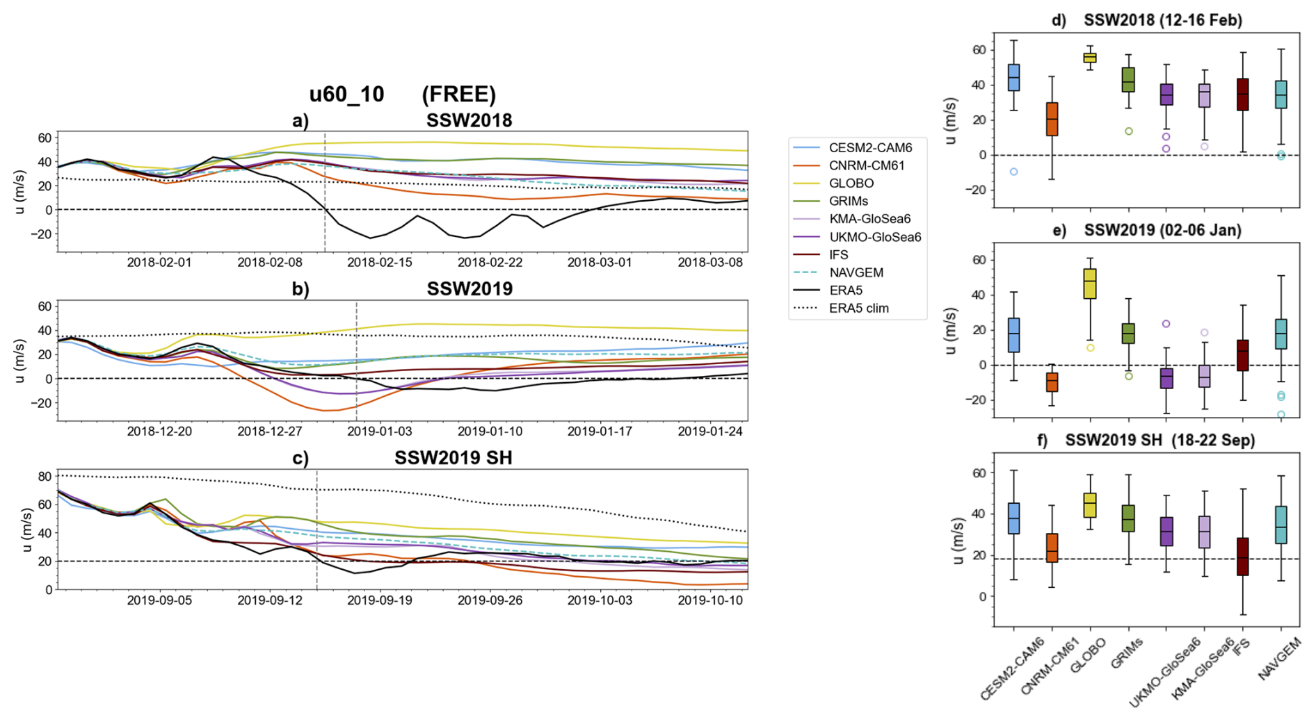
Figure 1 (left) Time evolution of the FREE ensemble mean of the zonal mean zonal wind (m s⁻¹) at 60° latitude and 10 hPa (u60_10) for each model (colored lines), ERA5 (black line), and ERA5 climatology (black dotted line) during the (a) SSW 2018, (b) SSW 2019 and (c) SSW 2019 SH. The vertical dashed line represents the timing of the fulfillment of the SSW criterion. (right) Boxplots showing the ensemble distribution of u60_10 for the dates around the occurrence of each SSW (indicated in the title). The size of the box and the horizontal black line represent the interquartile range (IQR) and the median value, respectively. Whiskers extend from the box to a distance of 1.5 times the IQR from the ends of the box. The horizontal dashed lines represent the threshold value of u60_10 to fulfill the SSW criterion.

Considering that the forecast lead time with respect to the SSW occurrence is very similar in the three experiments, the models experience the greatest challenge in predicting the SSW2018 (Fig. 1a and d vs Fig. 1b, c, e and f), consistent with previous literature (Butler et al., 2020; Rao et al., 2018, 2019, 2020b). In this case, the ensemble mean of nearly all models struggles even to simulate a deceleration of the PNJ, with less than 30 % of the ensemble members simulating an SSW in all models except for CNRM-CM6-1 (Table 3). NAVGEM also shows a relatively high number of ensemble members with an SSW, but most of them occur much later than in observations, i.e., late February and March, consistent with the weak values of the ensemble mean of u60_10 by that time. Indeed, for the 5 d period around the observed SSW onset date (12–16 February), easterly wind values are outside the 1.5 interquartile range (IQR) of the ensemble distribution of all models except for CNRM-CM6-1 (Fig. 1d). In contrast, the models' prediction skill for the two SSW events in 2019 is higher. For the NH event, all models except GLOBO simulate an SSW in many of the ensemble members (Table 3), but they tend to predict the event too early, as seen in the ensemble mean of u60_10 for CNRM-CM6-1 and both GloSea6 models (Fig. 1b). Consistently, during the few days around the central date of the SSW in ERA5, only GLOBO simulates westerly winds in all ensemble members (Fig. 1e). For the SH SSW, the deceleration of the PNJ is captured by the models over the first week. For the following days, whereas the PNJ in ERA5 continues decelerating even faster than in the previous days, models simulate a much weaker deceleration except for IFS and CNRM-CM6-1 (Fig. 1c). In these two models, the median of the ensemble distribution of u60_10 is close to the 20 m s⁻¹ threshold value for the 18–22 September (Fig. 1f).

Table 3 Percentage of ensemble members (%) that predict an SSW during the 45 d of the FREE experiment (first initialization).

3.2 Upward wave activity flux

Most of the model issues in simulating the three SSWs are consistent with model difficulties in reproducing the upward-propagating wave activity, as shown in the extratropical heat flux (HF) prior to the events in both the troposphere (300 hPa) and stratosphere (100 hPa) (Figs. 2–4). In the case of the SSW2018, the WN2 wave activity represented the predominant contribution to the enhancement of wave activity prior to this event (Ayarzagüena et al., 2018). The WN2 contribution consisted of a short but intense WN2 burst of wave activity in both the stratosphere and troposphere that started on 5 February as shown by ERA5 (black line Fig. 2a and b). However, the ensemble mean of HF in the forecast systems misses this strong enhancement of WN2 wave activity at both levels, particularly from 7 February (Fig. 2). This explains the general lack of deceleration of the PNJ from that date seen in Fig. 1a. The best performing forecast system is the CNRM-CM6-1 (orange line Fig. 2a and b): this is the only model with more than half of ensemble members simulating an SSW (62 %) and, consistently, it shows the strongest wave activity in the first days of the big pulse, particularly at 100 hPa (orange line Fig. 2a). Furthermore, it is the only model that reproduces a preceding secondary peak of wave activity on 2–5 February at 300 hPa.

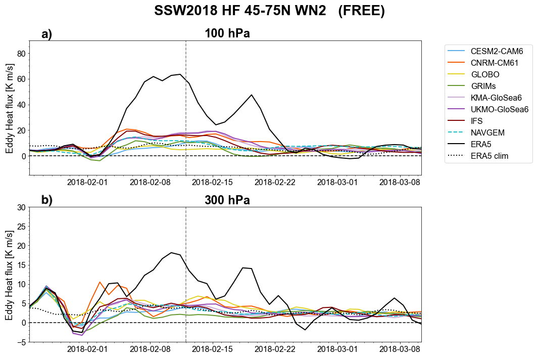
Figure 2 Time evolution of the ensemble-mean of the extratropical (45–75° N) eddy heat flux (K m s⁻¹) at (a) 100 hPa and (b) 300 hPa during the SSW 2018 for the WN2 component. The dashed vertical line denotes the date of the SSW.

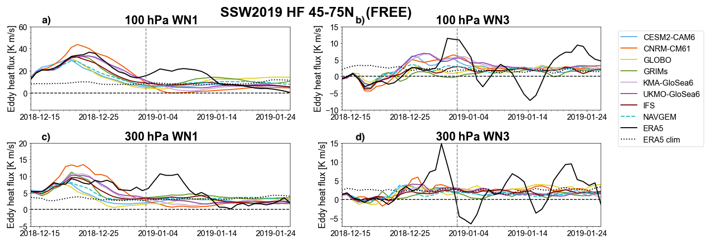
Figure 3 Time evolution for the NH SSW2019 of the ensemble mean of the extratropical eddy heat flux (K m s⁻¹) at 100 hPa for (a) WN1 and (b) WN3 wave components. (c) and (d) same as (a) and (b) but for the heat flux at 300 hPa. The dashed vertical line denotes the date of the SSW.

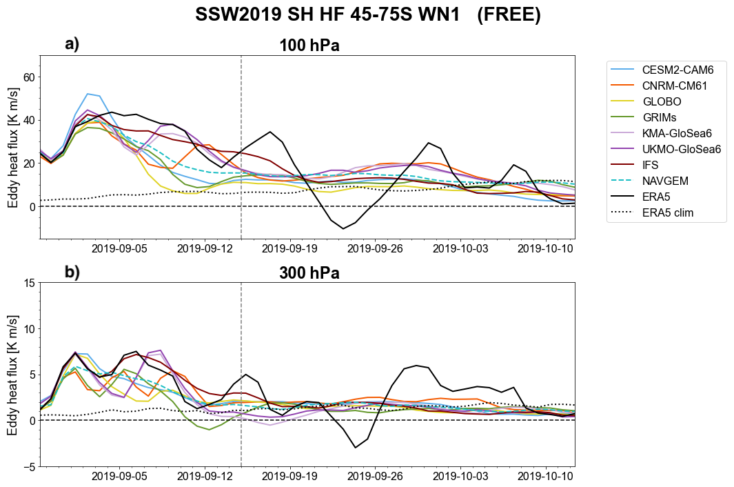
Figure 4 Same as Fig. 2 but for the SSW 2019 SH and the WN1 wave component. The heat flux values are multiplied by −1 to be comparable to the NH cases.

The SSW events of 2019 were both initiated by a moderate but persistent amplification of WN1 wave activity that is, in general, captured by the models (Figs. 3a and c and 4a and b). The results agree with the higher forecast skill for these two events. However, there are still model deviations from ERA5. The WN3 wave activity seems to play a relevant role for the occurrence of the NH event (Butler et al., 2020; Rao et al., 2019), but models struggle to simulate the WN3 burst around 4–5 d before the SSW onset date (Fig. 3b and d). In particular, the forecast systems either miss it or simulate a WN3 pulse both weaker and earlier than in ERA5. The latter happens in CNRM-CM6-1 (orange line) and both GloSea6 models (dark and light purple lines), which are the models with the highest SSW forecast skill, but with a too early SSW date (Fig. 1b). This may suggest that the simulation of the WN3 pulse might be linked to the forecasted timing of the SSW in each model. In this sense, Rao et al. (2019) and Butler et al. (2020) showed that during this event, the polar vortex first decelerated and shifted off the pole and then split. The wind reversal happened when the vortex split took place and has been linked to the peak of WN3 wave activity following the WN1 persistent burst (Rao et al., 2019). As for the SH event, in general, the WN1 burst is weaker in models than in the reanalysis, explaining the weaker modeled deceleration of the PNJ (Fig. 4a and b). Further, the models capture the WN1 magnitude in the stratosphere reasonably well initially, but they fail to simulate its long persistence (Fig. 4a). IFS is the model that performs best, particularly in terms of the persistence of the WN1 burst in both layers (brown line). This is also the model with the closest representation of the PNJ deceleration to observations (Fig. 1c).

3.3 Tropospheric circulation preceding SSWs

In previous subsections, we have identified a link between wave forcing and the deceleration of the PNJ, particularly, in relation to model biases. Given that the main sources of the wave activity are generally located in the troposphere, we extend our analysis to examine tropospheric conditions during the development of the three SSWs in the FREE experiment. Specifically, we focus on the period with intense tropospheric wave-driving in ERA5 for each of the three SSWs of study, i.e. the days corresponding to the strongest burst of upward-propagating wave activity at 300 hPa (3–13 February 2018; 18–30 December 2018; 1–10 September 2019). We investigate potential differences in tropospheric circulation in these time periods between members with a relatively weak versus a relatively strong PNJ at the time the SSW was observed in ERA5 (Table 2). To do so, Figs. 5–7 show in shading the difference of the composite map of Z500 anomalies of the 15 “weakest u” FREE members minus the 15 “strongest u” FREE members for each SSW. This analysis allows us to determine whether the tropospheric state was different between these two groups of ensemble members and so, played a role in the occurrence of SSWs. Further, it helps us identify tropospheric structures potentially influencing the likelihood for an SSW in the models. Since the difference plots of Z500 are not showing a complete pattern but just the differences in the tropospheric patterns between the two member groups, the figures also display in dark green contours the ensemble mean of Z500 of each model to help the interpretation of the results.

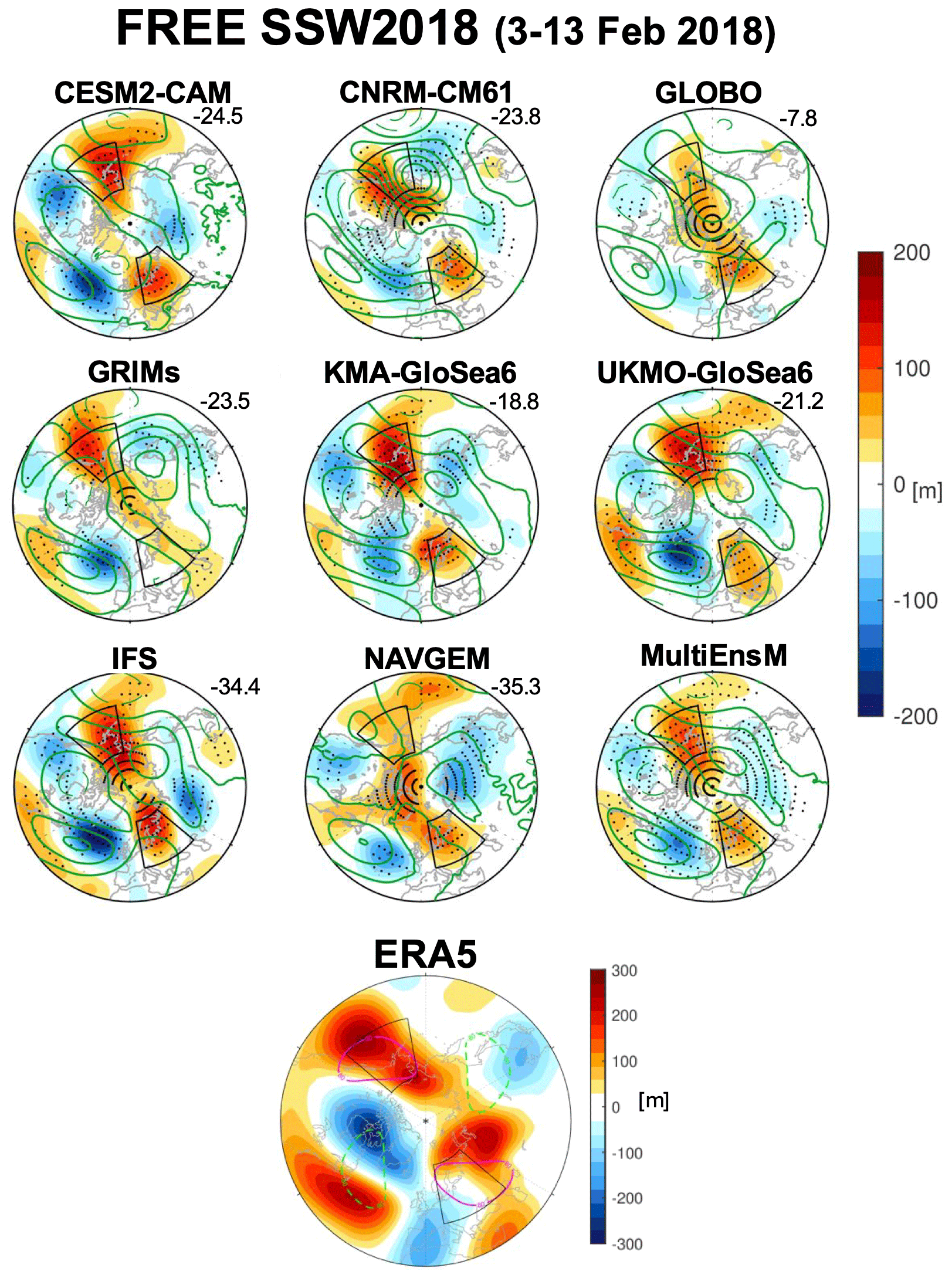
Figure 5 (upper panels) Composite maps of Z500 anomalies [m] during 3–13 February 2018 for the 15 members with the lowest values of u60_10 minus the 15 members with the highest values of u60_10 after the onset date of the SSW in ERA5 (12–16 February 2018). Dots indicate statistically significant values at the 95 % confidence level (t-test). The number below each model name corresponds to the difference in the averaged u60_10 [m s⁻¹] between the two groups of ensemble members. Black boxes delimit the area of the tropospheric precursors of the SSW assessed in Fig. 8. The dark green contours show the ensemble mean of Z500 anomalies for each model (interval: 90 m). (Bottom panel) Z500 anomalies in ERA5 for the same time period (3–13 February 2018). The magenta solid (green dashed) contours show the ERA5 climatological WN2 component of Z500 at ±80 m.

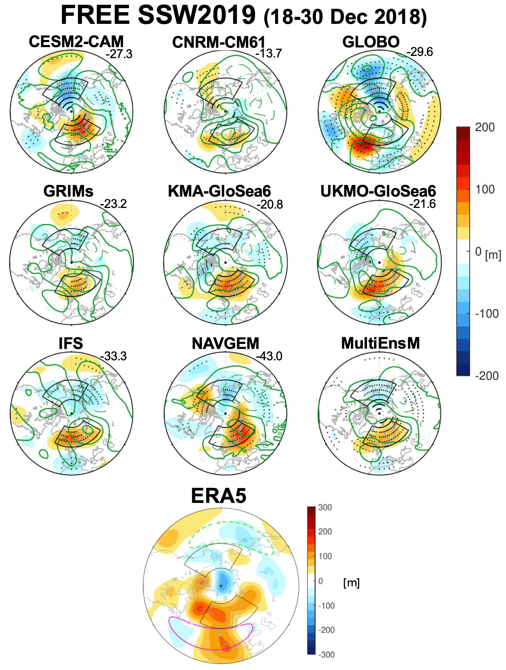
Figure 6 Same as Fig. 5 but for Z500 anomalies during 18–30 December 2018. The dates considered for selecting the members with the strongest u60_10 and weakest u60_10 are 2–6 January 2019. The dark green contours show the ensemble mean of Z500 anomalies for each model (interval: 60 m). The magenta solid (green dashed) contours in the bottom panel show the ERA5 climatological WN1 component of Z500 at ±80 m.

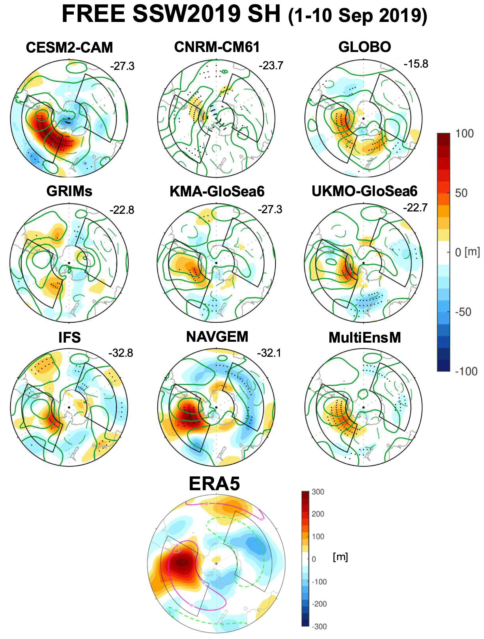
Figure 7 Same as Fig. 5 but for Z500 anomalies during 1–10 September 2019. The dates considered for selecting the members with the strongest u60_10 and weakest u60_10 are 18–22 September 2019. The dark green contours show the ensemble mean of Z500 anomalies for each model (interval: 80 m). The red solid (green dashed) contours in the bottom panel show the ERA5 climatological WN1 component of Z500 at ±40 m.

In the ERA5 plot for SSW2018 (Fig. 5, bottom row), we identify three centers of action (Alaskan blocking, East North American trough, and Ural blocking), with the Alaskan blocking as the strongest one. This blocking and the East North American trough are located close to a positive and a negative antinode of the stationary WN2 component of Z500, which would lead to a constructive interference of anomalous and climatological WN2 waves (Nishii et al., 2009; Garfinkel et al., 2010; Rao et al, 2018). In the FREE experiments, the ensemble mean of the Z500 anomalies (Fig. 5, dark green contours) differs notably from ERA5 in most models, with the strongest ridge over Eastern Asian or the North Pacific instead of Alaska. The result exemplifies the challenges in simulating this SSW in all forecast systems. However, the Z500 pattern associated with the weakest u60_10 displays, in general, similar features to ERA5 in both individual models and the multi-ensemble mean. Notably, the “weakest u” members show stronger Alaskan blocking compared to the “strongest u” members in all systems except for GLOBO. This agrees with Martius et al. (2009), who linked the occurrence of WN2 SSWs to blockings either over the Pacific or over both the Pacific and Eurasia. Nevertheless, in this case, the eastern American and Eurasia centers also appear to be key for the occurrence of the SSW2018, consistent with Karpechko et al. (2018). The model that does not show the Eurasian center of action in Fig. 5 (GRIMs) presents a very low number of ensemble members with an SSW. Furthermore, GLOBO displays a very weak Z500 pattern associated with the weakest u60_10. This result can be explained by the similar strong vortex state across members, as u60_10 differs by only ∼ 8 m s⁻¹ between the two ensemble groups. In summary, the tropospheric circulation was relevant for the deceleration of the vortex in February 2018 at least within the S2S systems analyzed here.

For both SSWs in 2019, the Z500 patterns of ERA5 are characterized by a strong center of positive anomalies and slight negative anomalies out-of-phase by 180° in longitude (Figs. 6 and 7). These patterns are consistent with the enhancement of WN1 wave activity leading up to these events as previously shown. More specifically, for the NH event, the ERA5 pattern shows a blocking over Greenland with positive Z anomalies extending over the North Atlantic basin and Scandinavia (Rao et al., 2019) (Fig. 6 bottom row), whereas in the case of the SH SSW, a strong ridge is apparent close to the Antarctic Peninsula (Rao et al., 2020a; Shen et al., 2020) (Fig. 7 bottom row). In the FREE experiment for the SSWs of 2019, we identify similar tropospheric patterns to ERA5 in the “weakest u” composites relative to the “strongest u” ones in both hemispheres (shadings in Figs. 6 and 7). Moreover, in these cases, the ensemble mean of anomalous Z500 (contours) also resembles the observed structure, particularly in the SH. In the NH SSW2019, the Greenland blocking preceding the SSW is mostly restricted to high latitudes, i.e., poleward of the stationary WN1 wave antinode, where constructive interference of waves would be less efficient if the climatological WN1 antinodes in the models were located similarly to those in ERA5. In the SH, the ensemble spread in the tropospheric pattern preceding the SSW is small, as indicated by the low values in the Z500 difference pattern (shading). In contrast, the spread in u60_10 is relatively large, with differences in u60_10 between “weakest u” and “strongest u” members ranging from 15 to 30 m s⁻¹ depending on the model. This suggests that, unlike the SSW2019, in addition to tropospheric forcing, other factors must have contributed to the development of the SSW2019 SH.

To summarize the results of this Section, we aim to establish a connection between tropospheric anomalies, wave amplification in the stratosphere and ultimately, the occurrence of the SSW. To do so, we analyze the pairwise relationships among these variables, following the sequence of processes that link tropospheric disturbances to polar vortex weakening. First, we correlate the combined main centers of action of the modeled Z500 patterns of Figs. 5–7 with the stratospheric upward-propagating wave activity, represented by the HF at 100 hPa (HF100). For each SSW, we define the areas characterized by substantial Z500 anomalies in the multi-ensemble mean of the “weakest u”-minus-“strongest u” Z500 patterns in Figs. 5–7. These areas are also close to the antinodes (ridge or trough) of the climatological WN1/WN2 waves in ERA5. The Z500 anomalies are then averaged over these regions denoted by black boxes in Figs. 5–7 and combined by computing the mean of the absolute values of the anomalies for each center. The HF100 is computed for the predominant wavenumber and averaged during its strongest burst in ERA5 (6–14 February 2018; 21 December 2018–3 January 2019; 2–15 September 2019). Additionally, we assess the relationship between HF100 and the u60_10 around the SSW onset date.

Figure 8a–c present scatter plots of the correlation coefficients corresponding to the pairwise relationships for each model and SSW event. These correlations are generally statistically significant, confirming the linear relationship among the three variables for all the SSW events analyzed in this study (see also Fig. S1). However, the strength of the relationship between tropospheric precursors and HF100 varies depending on the event. For SSW2018, the link between WN2 upward-propagating wave activity and tropospheric precursors is, in general, weaker compared to the other two SSWs. Moreover, there is a substantial inter-model variability in the value of the correlation coefficient, ranging from 0.38 in GRIMs to 0.82 in UKMO-GloSea6 (Fig. 8a). In contrast, for SSW2019, WN1 wave activity in the lower stratosphere appears strongly correlated with the tropospheric precursors and models even agree on the value of the correlation coefficient (around 0.75) (Fig. 8b). Similar behavior is found for SSW2019 SH, but with weaker correlations and a broader spread across models (∼ 0.60 to 0.77 for most of the models) (Fig. 8c). An exception is detected for the SSW2019 in CNRM-CM6-1, where HF100 and Z500 are decoupled (Fig. 8b). This model exhibits the strongest HF100 (Fig. 3a), but the wave burst starts earlier than in ERA5 and in the other models, and thus, the different timing of the wave amplification may explain the lack of coupling in this model.

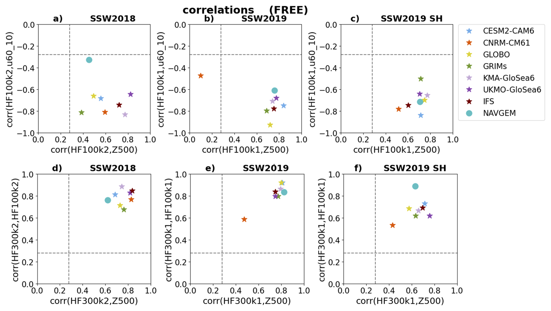
Figure 8 (a)–(c) Scatter plot of correlation coefficients across all members of each ensemble of u60_10 and HF at 100 hPa for the predominant wavenumber vs the correlation of this HF and tropospheric precursors identified in Figs. 5–7 at 500 hPa (see more details in the text). The gray dashed lines indicate the threshold values for statistically significant correlation coefficient values at the 95 % confidence level (t-test). (d)–(f) Same as (a)–(c) but for the correlation of HF at 100 and 300 hPa for the predominant wavenumber vs the correlation of HF at 300 hPa and tropospheric precursors.

While the relationship between tropospheric precursors and HF100 varies across SSW events, the correlation between the stratospheric variables remains approximately the same for the three events. u60_10 shows a strong negative correlation with HF100, with correlation coefficients typically ranging from −0.55 to −0.85. Exceptions are found for SSW2018 in NAVGEM and for SSW2019 in CNRM-CM6-1. In the case of NAVGEM, several factors may contribute to the low correlation, potentially including biases in wave-mean flow interactions, since this model also shows a relatively low correlation between u60_10 and HF100 during SSW2019 (Fig. 8a and b). For CNRM-CM6-1, as previously discussed, the timing of stratospheric processes is substantially earlier than in ERA5, with all ensemble members simulating an SSW around 25 December 2018.

These results indicate that a strong correlation between the two stratospheric variables does not necessarily imply a strong coupling between HF100 and the tropospheric precursors. To understand this coupling more thoroughly, we analyze the potential linkage between the tropospheric precursors, the upper tropospheric wave forcing (predominant WN HF300) and the lower stratospheric one (predominant WN HF100) by correlating Z500-HF300 and then, HF300- HF100 and contrasting both correlations in Fig. 8d–f. In the case of the SSW2019, all S2S systems exhibit strong correlations between Z500 and WN1 HF300 as well as between WN1 HF100 and WN1 HF300, with all points clustered in the upper right quadrant of the plot. These results confirm that tropospheric precursors highly influence the lower stratospheric wave activity. Thus, inter-model differences in vortex deceleration associated with SSW2019 may be related to variations in wave-mean flow interactions as well as differences in the strength of tropospheric precursors. For SSW2018, there is also a generally strong coupling between the stratospheric variables. However, the correlations between Z500 and WN2 HF300, and between WN2 HF100 and WN2 HF300 show a wider spread compared to SSW2019, slightly larger in the HFs case. This together with the low WN2 HF100–Z500 correlation suggests that the stratospheric wave activity might be modulated by additional sources beyond the troposphere, at least in some of the models, such as non-linear wave processes in the stratosphere. Indeed, CNRM-CM6-1, the model with the largest number of ensemble members with an SSW and the strongest burst of WN2 wave activity at 100 hPa, shows a very high correlation between WN2 HF300 and Z500 similar to IFS or UKMO-GloSea6, but, unlike these systems, the correlations in CNRM-CM6-1 weaken substantially between the upper-tropospheric and lower-stratospheric forcing.

The most intriguing results emerge for the SH event. While the correlation between WN1 HF100 and Z500 remains strong and consistent across most models, the correlations involving intermediate variables, i.e. HF300–Z500 and HF300–HF100, are generally lower than in the two NH events. This relatively weak link between upper-tropospheric and lower-stratospheric wave forcing may also point to a non-negligible role of the stratosphere in driving the SSW, similar to SSW2018. In particular for this case, the filtering effect of the stratospheric winds might be a potential driver given the very strong values of some ensemble members (Fig. 1f). Regarding the WN1 HF300–Z500 relationship, Fig. 7 shows that the tropospheric forcing consists of short pulses from other wave components, some of which may be included within the tropospheric precursors. The compensating effects leading to the strong WN1 HF100–Z500 correlation warrant further investigation, but such an analysis lies beyond the scope of this study.

In short, our analysis suggests that SSW2019 is driven by tropospheric precursors while the stratospheric state seems to play a larger role in driving SSW2018 and SSW2019 SH. This role will be assessed in more detail in the next Section.

4 Influence of the stratospheric state on triggering mechanisms of the three SSWs

So far, we have assessed model performance in capturing the triggering mechanisms of the SSWs in the FREE experiment and hypothesized about the role of the troposphere/stratosphere in these mechanisms. Next, we investigate in more detail the influence of the zonally symmetric stratospheric state on initiating the three SSWs by means of the NUDGED and CONTROL experiments.

First, we analyze the stratospheric influence on the enhancement of upward-propagating wave activity prior to the SSWs. Figure 9 shows, for each model, the ensemble distribution of total eddy heat flux at 100 and 300 hPa averaged during the strongest peak of HF at each level (indicated in the figure). Additionally, the distribution of the ensemble means of all models is also displayed in the figure in gray. Overall, the general deviations of the tropospheric and stratospheric heat fluxes in the FREE experiments from the reanalysis are also shared by the NUDGED and CONTROL experiments. For instance, the underestimate by the models of the enhancement of stratospheric wave activity prior to the SSW2018 in FREE is evident in the NUDGED and CONTROL runs too. This might suggest a minimal influence of the stratospheric state on upward wave propagation.

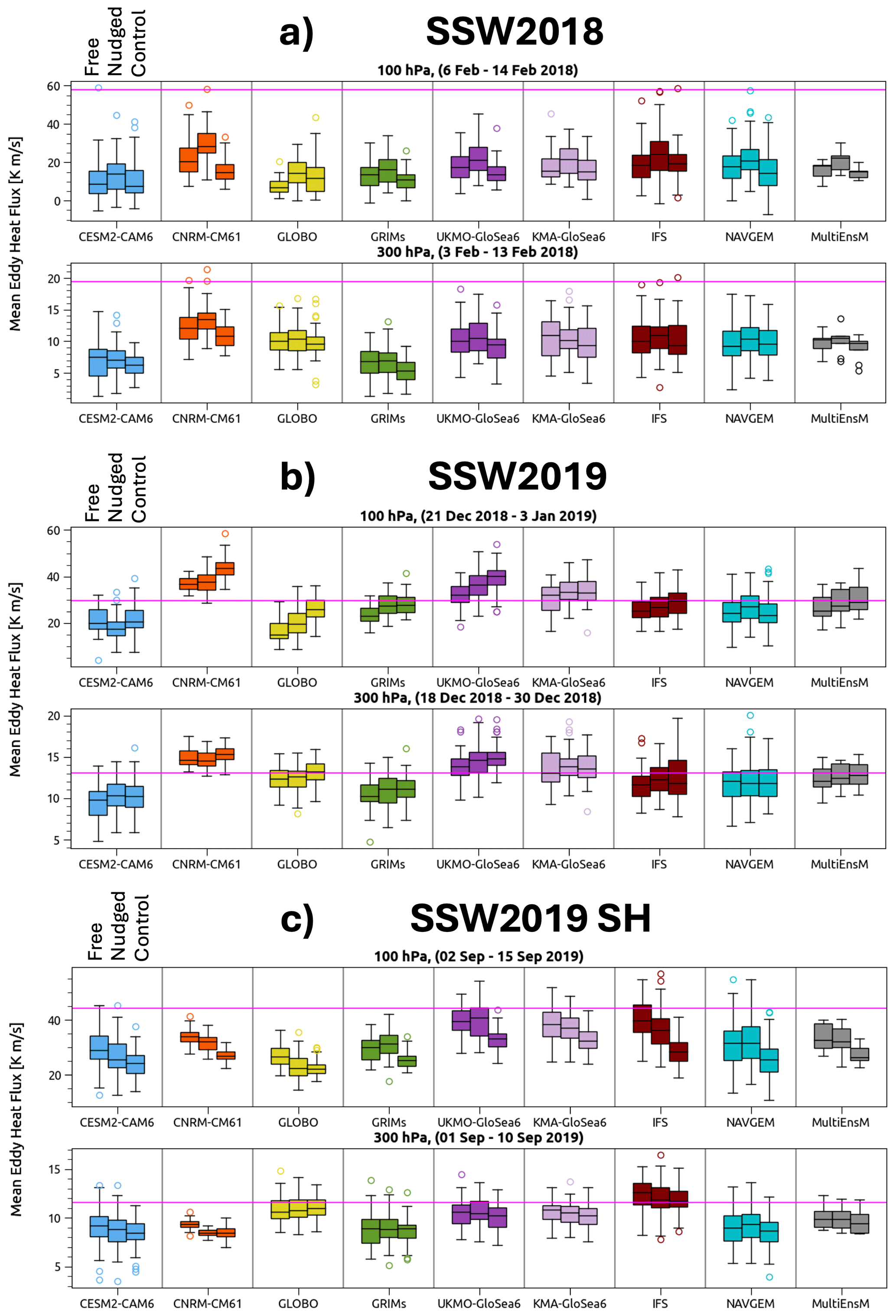
Figure 9 Boxplots showing the ensemble distributions of eddy heat flux (HF) at 100 and 300 hPa and 45–75° for the period with the strongest value of HF preceding each SSW for all models and multimodel mean (MultiEnsM), and the different experiments (FREE, NUDGED, and CONTROL runs). The interquartile range (IQR) is represented by the size of the box and the horizontal black line corresponds to the median value. Whiskers extend from the box to a distance of 1.5 times the IQR. Outliers (colored circles) are defined as points with values greater than 1.5 times the IQR from the ends of the box. ERA5 values are represented by horizontal magenta lines.

Nevertheless, when comparing results in the NUDGED and CONTROL experiments, some differences appear, although mostly in the stratospheric wave activity. Prior to the SSW2018, the multimodel mean of HF100 in the NUDGED run has a value of 21.0 K m s⁻¹, compared with 14.5 K m s⁻¹ in the CONTROL run. Thus, HF100 in the NUDGED run is 144 % of that in the CONTROL run; in other words, it is 44 % stronger than in the CONTROL run (Fig. 9a). Similarly, the HF100 preceding the SSW2019 SH is also stronger in the NUDGED (32.4 K m s⁻¹) than in the CONTROL experiment (27.5 K m s⁻¹), but only by 17.8 % (Fig. 9c). The sign of the HF100 difference agrees with linear wave theory for the SH event because a weak but still westerly polar vortex, as in the NUDGED experiment, favors upward wave propagation. For the NH SSW2019 case, the ensemble mean values of HF100 are very similar in the NUDGED and CONTROL experiments (28.5 vs 30.9 K m s⁻¹, i.e. the difference is only 8 %) (Fig. 9b). The result points to a large tropospheric influence on the stratospheric wave activity leading to the occurrence of this SSW. This also confirms results of Fig. 8 for SSW2019 that showed the strongest correlation between the tropospheric precursors and HF100 for almost all models, with values around 0.75. Despite the similarity in HF100 in the NUDGED and CONTROL experiments, it is worth highlighting that most of the models tend to simulate higher values in CONTROL than in NUDGED. This might seem to contradict the linear wave theory mentioned before. A potential explanation might be related to the effects of WN1-WN3 wave interactions (Shi et al., 2017). In the case of the NUDGED runs, the very weak PNJ favors the propagation of the WN3 wave burst into the stratosphere close to the SSW central date. When this wave activity is enhanced, the WN1 wave activity is reduced in most models similar to the evolution in ERA5 (Fig. 3). In contrast, the PNJ is stronger in the CONTROL runs, which would make it difficult for the WN3 wave activity to propagate in the stratosphere. More analysis is required to understand this, but it is beyond the scope of this study.

Interestingly, the dispersion of HF values across ensemble members in all models is very similar in the three experiments and the three events, suggesting that the stratospheric state does not modulate the variability of HF. The stratosphere does not seem to remarkably affect the tropospheric wave activity either, as we do not find relevant differences in HF at 300 hPa across experiments.

The previous statements are based on the overall behavior observed across all models. However, although the zonal mean state in the sensitivity experiments is the same in all models, the performance of specific forecast systems varies. Notably, the CNRM-CM6-1 system stands out for the SSW2018 (Fig. 9a). Unlike the other models, the median value of the HF100 in the NUDGED experiment of CNRM-CM6-1 is substantially stronger than in the CONTROL one, with no overlap in their interquartile ranges. More importantly, only CNRM-CM6-1 shows an impact of the stratospheric state on the tropospheric wave activity, as the NUDGED median exceeds the CONTROL interquartile range of HF at 300 hPa. Further, CNRM-CM6-1 shows the strongest HF values at 100 and 300 hPa in both the NUDGED and FREE experiments and consistently, the highest number of ensemble members predicting an SSW (62 %) in FREE. These results suggest that in a system that more skillfully predicts the factors that lead to this SSW, the stratospheric state does indeed have an influence on the troposphere. Further evidence will be presented next that indicates that the stratospheric state is having an influence on the tropospheric circulation patterns that may have played a relevant role in triggering the SSW2018.

Next, we explore the influence of the stratospheric state on the tropospheric structures that preceded the three SSWs. The spatial patterns of Z500 across the three experiments are very similar, suggesting that the stratospheric state does not remarkably alter the tropospheric circulation prior to these three SSWs (contours in Figs. 5–7 for the FREE experiment and S2–S4 for NUDGED and CONTROL). Figure 10 shows the ensemble distribution of the combined Z500 anomalies over the precursor regions used in Fig. 8 and identified with black boxes in Figs. 5–7. The results are consistent with the intensity of HF at 300 hPa in Fig. 9. The Z500 anomaly amplitudes in FREE tend to be weaker than those in ERA5 except for the SSW2019 (Fig. 10b). In the case of SSW2018 the median value of these amplitudes is exceptionally weak in all systems but CNRM-CM6-1, which is close to ERA5 (Fig. 10a). In contrast, the median values of Z500 anomaly amplitudes in FREE prior to SSW2019 SH, although lower than those in ERA5, are closer to reanalysis than in SSW2018.

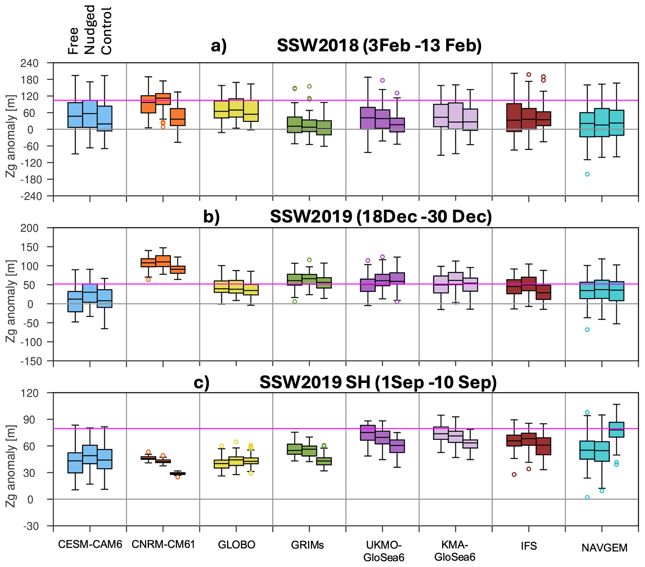
Figure 10 Same as Fig. 9 but for the combined Z anomalies at 500 hPa averaged over the areas of the tropospheric precursors of SSWs highlighted in Figs. 5–7. ERA5 values are represented by horizontal magenta lines.

When comparing NUDGED and CONTROL experiments, the results confirm that the impact of the stratospheric state on the intensity of the tropospheric circulation preceding SSWs is also small for the majority of models. Indeed, the two experiments show virtually identical results for each NH SSW in terms of median values and variability. For the SSW2019 SH, although not always significant, all systems except for NAVGEM tend to show a higher amplitude of the tropospheric precursors in NUDGED than in CONTROL runs. This is mainly due to the stronger center over the Antarctic Peninsula in the NUDGED experiment, as revealed by the composite maps of Z500 anomalies prior to the SSW (Fig. S4). Since a weak vortex induces positive Z500 anomalies over this center (Turner et al., 2012) and the vortex was weak before the SSW in ERA5 (Fig. 1c), the troposphere in the NUDGED experiment might already be affected by the weak polar vortex influence. This also agrees with Jucker and Reichler (2023) who found that the SH polar vortex typically starts to decelerate more than 50 d before SSWs and consistently, very strong positive anomalies over the Antarctica Peninsula appear in the troposphere one month before the occurrence of an SSW. When analyzing individual S2S systems, only CNRM-CM6-1 displays large differences between the two experiments for all three SSWs. In particular, for the SSW2018, the ERA5 value lies within the interquartile range of the values of the NUDGED ensemble of this model, whereas the CONTROL experiment resembles the weak values of other models such as KMA-GloSea6, IFS, or CESM2-CAM6 (Fig. 10a). More importantly, the NUDGED ensemble shows a notable reduction in spread compared to CONTROL and FREE experiments (Fig. 10a). This means that the stratospheric state exerts control on the tropospheric circulation, which only this model is able to capture. This influence is also evident in the CNRM-CM6-1 FREE run as it shows stronger values than the other models and might be key for triggering the SSW2018 event, as already suggested by the HF results. For the other two events, the Z500 anomalies in the CNRM-CM6-1 NUDGED are stronger than in CONTROL and similar to FREE. However, the ensemble spread is not very different across experiments and the model values differ from ERA5. Thus, the stratospheric control over the troposphere might not be as important for triggering these two SSWs as for SSW2018.

5 Study of the wave propagation and amplification prior to SSW2018

In the previous Sections, we have detected hints that the stratospheric state had the largest influence on the occurrence of SSW2018 (Figs. 9 and 10); a deeper analysis of this event with the SNAPSI experiments will thus help to clarify the role of the stratosphere in triggering this SSW. In addition, the SSW2018 is the most difficult event for the models to predict, so this analysis may also help to understand the models' issues with simulating the wave activity propagation. In the following, we perform a specific analysis of the wave propagation prior to the SSW2018.

5.1 Analysis of the upward wave propagation in the FREE experiment

We start by analyzing the vertical propagation of the wave activity in ERA5 and the FREE experiment of the models and the simultaneous evolution of the PNJ. Figure 11 displays the time evolution of the F_z (shading) in both the troposphere and stratosphere for the predominant wave component (WN2). The zonal-mean zonal wind at 60° N (u60) is also included in contours. For brevity, we only show results for four models: CNRM-CM6-1, KMA-GloSea6, GRIMs, and IFS. CNRM-CM6-1 has the best forecast skill of this event; KMA-GloSea6 shows results that are close to those from UKMO-GloSea6; GRIMs is included as an example of a low-top model since it performs similarly to the other two low-top models (CESM2-CAM6 and GLOBO). Lastly, IFS is an example of an intermediate model in terms of forecasting this SSW. To better understand the stratospheric state and the wave propagation at certain key times, the Eliassen-Palm flux (F, arrows) is shown in Fig. 12 for the WN2 wave component at specific periods together with the zonal-mean zonal wind (shading).

Figure 11 Time evolution of the vertical component of the Eliassen-Palm flux (F_z, shading (kg s⁻²)) averaged over 50–70° N for the WN2 component and the zonal mean zonal wind at 60° N (black contours, m s⁻¹) from 25 January until 10 March 2018 in (a) ERA5 and the FREE experiment of (b) CNRM-CM6-1, (c) KMA-GloSea6, (d) GRIMs and (e) IFS. The vertical magenta line indicates the date of the SSW in ERA5. The yellow (green) vertical dashed lines delimit the 3–5 (6–8) February period.

Figure 12 (a) Eliassen-Palm flux (arrows, m³) for the WN2 wave component and zonal mean zonal wind (shading) for 3–5 February 2018 in ERA5. (b)–(e) Same as (a) but for the FREE experiment of CNRM-CM6-1, GRIMs, KMA-GloSea6 and IFS. (f)–(j) Same as (a)–(e) but for 6–8 February 2018.

A first burst of wave activity is observed by late January in ERA5 and all models. The associated F_z maximum is mainly restricted to the troposphere (Fig. 11a). In the stratosphere, weaker positive F_z appears some days later, indicating that it propagates from the troposphere to the stratosphere, where it leads to a vortex weakening. After a period without upward wave propagation, the polar vortex in ERA5 re-intensifies rapidly in the upper and middle stratosphere in early February (3–5 February, delimited by vertical yellow lines in Fig. 11) and shifts poleward with a PNJ centered at around 68° N in that 3 d period, with almost no vertical tilt from 100 to 3 hPa, but strong curvature above that level (shading in Fig. 12a). This vortex configuration resembles a wave cavity favoring the resonant excitation of waves in the mid-stratosphere and channeling waves towards the pole in the upper stratosphere, which decelerate the PNJ at those levels (arrows in Fig. 12a). The easterly phase of the equatorial quasi-biennial oscillation (QBO) in the middle stratosphere (40–10 hPa) also contributes to build a barrier for equatorward wave propagation. This stratospheric configuration is characteristic of the “preconditioned state” of WN2 SSW events (Palmer, 1981; Albers and Birner, 2014). However, this configuration is not simulated by the models. Actually, early February (3–5 February) is the time when the forecast systems start to deviate from the reanalysis. The strengthening of u60 is poorly simulated by the models (Fig. 11b–e) and the polar vortex structure is also different, with a PNJ core shifted southward and downward with respect to that in ERA5 (shading in Fig. 12b–e). Consequently, forecast systems display stronger equatorward wave propagation, particularly in the upper stratosphere (arrows in Fig. 12b–e) compared to ERA5.

In the next 3 d period (6–8 February), the atmospheric state and the upward wave propagation undergo substantial changes, both in ERA5 and forecast systems. In ERA5 the PNJ is weaker than before (Figs. 11a and 12f), and its maximum has descended to the middle stratosphere (Fig. 12f). This configuration allows equatorward wave propagation at mid-latitudes (up to 60° N) and more importantly, upward wave propagation at higher latitudes (60–72° N), favoring in turn the deceleration of the PNJ (Fig. 12f). Consistently, a second and stronger burst of wave activity beginning on 6 February is observed in ERA5 in Fig. 11a (vertical green lines delimit the period). This burst occurs simultaneously in the troposphere and stratosphere and persists until the reversal of u60 on 12 February in most of the stratospheric column, when the wave activity starts to decline (Fig. 11a). The models simulate a totally different atmospheric state, with a strengthening of the PNJ in 6–8 February, particularly in GRIMs (Fig. 12g–j). Indeed, although models display an intensification of the stratospheric wave activity, it is much weaker than that in ERA5 and mostly restricted to latitudes south of 60° N except in CNRM-CM6-1 (Fig. 12g–j). In the troposphere, F_z is also weaker than in ERA5, particularly in CNRM-CM6-1 (Figs. 11b–e and 12g–j). Moreover, in the following days the wave enhancement in the stratosphere is not as intense and as simultaneous in the whole atmospheric column as that in ERA5 (Fig. 11b–e), potentially explaining the absence of an SSW in most of the models and consistent with Fig. 2. Considering that the polar vortex state in the models starts to deviate from that in ERA5 at the same time or even at earlier stages than F_z, the stratospheric state might be important for the occurrence of the rapid enhancement of wave activity leading to the occurrence of the SSW2018.

5.2 Influence of the stratospheric state on wave propagation

So far, we have seen that the wave propagation differs between the FREE model ensembles and ERA5 and these discrepancies are consistent with differences in the background state. One may hypothesize that this could explain the weak wave activity in the stratosphere simulated by the models. Next, we check if this is mainly due to the zonally symmetric stratospheric state by comparing the time evolution of F_z in the NUDGED and FREE experiments in Fig. 13, as the zonal mean stratospheric state in the NUDGED experiment corresponds to the observations.

Figure 13 Time evolution of the vertical component of the Eliassen-Palm flux (F_z, shading (kg s⁻²)) averaged 50–70° N for the WN2 component and the zonal-mean zonal wind at 60° N (contours, m s⁻¹) from 25 January until 10 March 2018 in the NUDGED-minus-FREE experiments of (a) CNRM-CM6-1, (b) KMA-GloSea6, (c) GRIMs and (d) IFS. Dots indicate non-statistically significant values at the 95 % confidence level (t-test). The vertical magenta line indicates the date of the SSW in ERA5.

In general and similar to Fig. 9, in the days before the SSW we do not find markedly stronger upward-propagating wave activity in the NUDGED experiment compared to FREE (Fig. 13), except in CNRM-CM6-1. The period of vortex intensification on 3–5 February in NUDGED that is not captured by the FREE runs can be identified by the positive NUDGED-minus-FREE differences in u60. After that, the FREE experiments do not capture the intensification of the wave activity in the stratosphere that was present in ERA5 from 6 February (Fig. 11). Interestingly, the NUDGED experiments of KMA-GloSea6 and GRIMs show even weaker wave activity in the first days of this period than the FREE ones. In CNRM-CM6-1 and IFS, F_z shows larger values in NUDGED than in FREE, although in the latter it is only statistically significant above 100 hPa. More importantly, from 8 February none of the models show stronger wave activity in the troposphere in the NUDGED run than in the FREE one. Indeed, if they show a significant NUDGED-minus-FREE difference in those levels, it is negative, as seen in CNRM-CM6-1 and IFS (Fig. 13a and d). In contrast, in the stratosphere (in particular, from 50 hPa) there is, in most of the models, an enhancement of upward-propagating wave activity. Notably, this enhancement is not connected to a previous enhancement in the troposphere, i.e., the amplification occurs in the stratosphere itself, which constitutes another hint of wave resonance. These results suggest that the differences in the representation of the zonally symmetric stratospheric state in models with respect to ERA5 (Figs. 11 and 12) contribute to the lack of the strong WN2 burst in the stratosphere. However, this contribution is smaller than the total model bias; namely, the models in the NUDGED experiment still simulate much weaker upward wave flux in the stratosphere than ERA5. Further, the mentioned wave resonance might be characteristic of the vortex breakdown and thus approximately captured by the NUDGED experiment. However, it is not the cause of this breakdown, considering that the upward wave flux is not comparable to observations.

In the previous figures, the upward wave activity flux in the stratosphere has been found to be partially modulated by the zonal mean stratospheric state. As a final step, we assess the influence of this state on the net EP flux budget in the polar stratosphere during the strongest peak of wave activity in the stratosphere (6–14 February) (Fig. 14, see Sect. 2.2.2 for calculation details). Figure 14 presents the ensemble distribution of the net EP flux for all wavenumbers (Fig. 14a) and WN2 only (Fig. 14b) in the polar stratosphere (55–90° N and 100–10 hPa) along with the different terms of the latter, i.e., the integrated F_z at 100 hPa (F₁₀₀) and 10 hPa (F₁₀) and the F_y at 55° N (F_55N) (Fig. 14c–e). The positive values of the net EP flux in ERA5 indicate strong EP flux convergence for all wavenumbers (horizontal magenta line in Fig. 14a) and for WN2 only (Fig. 14b) in the stratosphere, consistent with a strong deceleration of the PNJ. There is a remarkable upward WN2 EP flux at 100 hPa in agreement with Figs. 2, 9, and 11 (horizontal magenta line in Fig. 14c). Conversely, the upward flux at 10 hPa (F₁₀) and the equatorward EP flux at 55° N (F_55N) display much weaker values, consistent with the strong convergence of wave activity in the box (Fig. 14d and e, respectively). Thus, the F₁₀₀ constitutes the main contribution to the strong convergence of WN2 wave activity in the polar stratosphere and, ultimately, to the occurrence of the SSW2018. In the FREE experiment, models underestimate all components of WN2 EP flux budget, with the most pronounced bias in F₁₀₀ (Fig. 14c), resulting in relatively low positive values of net EP flux for WN2 (Fig. 14b) and thus small impact on the PNJ strength compared with ERA5.

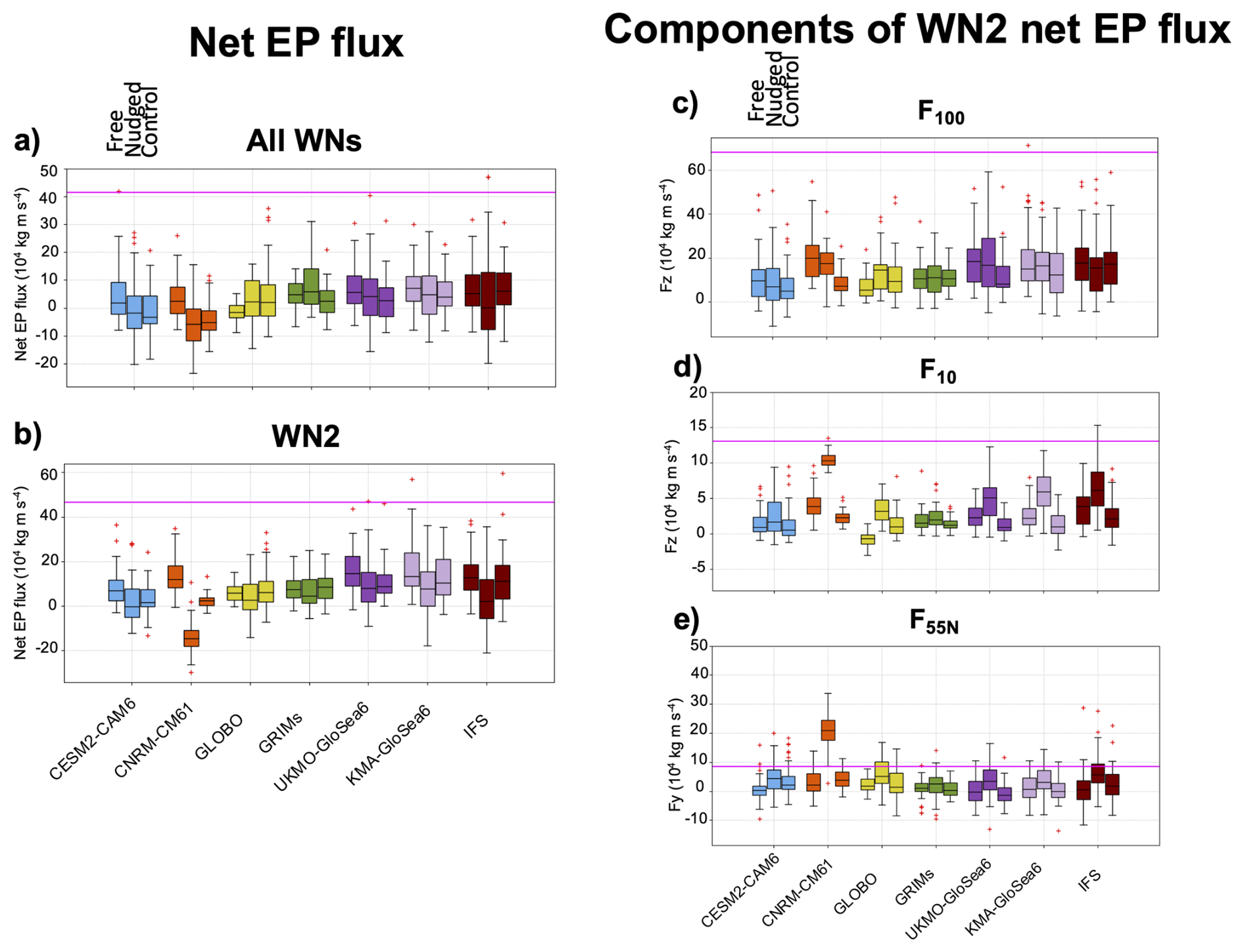
Figure 14 Boxplots of net EP flux in the polar stratosphere (100–10 hPa, 55–90° N) for all wavenumbers (a) and WN2 (b) and its components (c)–(e) averaged during 6–14 February 2018. The interquartile range (IQR) is represented by the size of the box and the horizontal black line corresponds to the median value. Whiskers extend from the box to a distance of 1.5 times the IQR. ERA5 values are represented by horizontal magenta lines. The outliers are indicated by red crosses.

Focusing now on the effects of the stratospheric state on the EP flux budget, we do not find large differences in the magnitude of the net budget across the sensitivity experiments, although three models (CNRM-CM6-1, IFS and KMA-GloSea6) simulate even lower values in NUDGED than in CONTROL runs. The individual terms, particularly the vertical ones, also remain much weaker than in ERA5. Nevertheless, both F_55N and F₁₀ appear to be modulated by the stratospheric state, as all models show higher values in the NUDGED than in the CONTROL runs (Fig. 14d and e), explaining the relatively lower net flux in NUDGED. For F₅₅, this difference is statistically significant only in CNRM-CM6-1 (Fig. 14e) and agrees with the increase in the equatorward flux already detected in the 6–8 February in ERA5 associated with the observed weaker vortex (Fig. 12f). However, the strongest modulation occurs for F₁₀. This term is statistically significantly stronger in NUDGED than in CONTROL in the four high-top models (CNRM-CM6-1, both GloSea6s models and IFS), consistent with the increase of F_z above 50 hPa around 9 February (Fig. 13), which was not connected to a corresponding enhancement in the troposphere. The combined results of F_55N and F₁₀ imply that the zonal mean stratospheric state amplifies wave activity in the middle and upper stratosphere, considering that the lower stratospheric wave activity (F₁₀₀) remains largely unchanged across the two sensitivity experiments in most models (Fig. 14c). This has been confirmed by the differences in the EP flux distribution averaged over the same period (6–14 February) (Fig. S5). A final remark is the impact of the stratospheric state on the spread of the net EP flux and its components: In CNRM-CM6-1 and UKMO-GloSea6, the spread of all the analyzed quantities is narrower in the CONTROL than in the NUDGED experiments. This likely occurs because the stronger vortex in CONTROL imposes greater constraints on wave propagation.

To sum up, consistent with the other results of this Sect. 5, the dominant contribution to the strong convergence of net EP flux prior to SSW2018 arises from the lower stratospheric upward-propagating wave activity (F₁₀₀), but models largely underestimate it. Overall, the stratospheric state does not remarkably affect F₁₀₀, but we find hints that the zonally symmetric stratospheric state does modulate the wave activity at higher levels, amplifying it in agreement with a wave resonance process.

6 Summary and discussion

In this study, we perform a multimodel analysis of triggering mechanisms for SSWs depicted by S2S forecast systems. In particular, we take advantage of the new SNAPSI experiments from eight S2S forecast systems to systematically assess, for the first time, the role of the stratospheric state in triggering the boreal SSWs of 2018 (SSW2018) and 2019 (SSW2019) and the austral minor warming of 2019 (SSW2019 SH). The SNAPSI experiments represent a unique set of experiments specifically designed to isolate the effects of the zonally symmetric stratospheric state on the atmosphere, with the stratospheric state either evolving freely, following the climatology, or following the specific SSW conditions depending on the experiment.

These are the main conclusions from the analysis of the SNAPSI experiments:

• Forecast systems show a similar quality for predicting the upward wave activity flux in the troposphere and stratosphere prior to the three SSWs as for predicting the events themselves, in agreement with Taguchi (2018). Specifically, while the forecast systems are able to simulate the moderate but persistent WN1 wave activity preceding both SSW events of 2019 (SSW2019 and SSW2019 SH), they fail to capture the intense burst of WN2 wave activity that occurred before the SSW2018. Similarly, the models have the most difficulty in simulating the SSW2018, while their performance is relatively good for the other two SSWs.

• The forecast systems perform better at simulating the tropospheric circulation before the two SSWs of 2019 than before the SSW2018. In particular, the models capture the location (near the antinodes of the climatological WN1 Z500 wave) and intensity of the blocking highs preceding the two SSWs of 2019. In contrast, tropospheric precursors prior to SSW2018 exhibit weaker intensity in models than in ERA5 and are not even simulated in many ensemble members. This explains why the models could simulate the enhancement of wave activity in the troposphere through probably constructive interference of anomalous and climatological waves in the case of the 2019 events, while failing to predict this enhanced tropospheric wave activity for the 2018 case.

• The zonal mean stratospheric state does not seem to drastically affect the variability and mean values of the upward wave activity flux and tropospheric circulation anomalies prior to SSWs. The largest influence is identified for the stratospheric wave activity, although this modulation depends on the event characteristics. The relative role of the stratospheric state in triggering the SSW also varies by event.

• The SSW2018 was preceded by a very strong burst of WN2 wave activity that occurred simultaneously in the troposphere and stratosphere. The poleward-shifted polar vortex state may have conditioned the occurrence of this strong burst, but the models were not able to capture it in the FREE experiment. Even when the zonally symmetric stratospheric state is imposed, the forecast skill of this burst in the lower stratosphere is still low, indicating that other factors such as the tropospheric precursors are fundamental for the strong enhancement of WN2 in the whole column.

Overall, the results suggest that both tropospheric and stratospheric processes play a role in initiating an SSW, although their relative contributions vary by event. First, the wave forcing and tropospheric precursors are different for each case. Second, the stratospheric state is also different, including different intensities of the polar vortex relative to climatology and different QBO states, which influence the wave activity in the stratosphere. The SSW2019 represents a clear example of an event mainly driven by tropospheric precursors in agreement with Matsuno (1971). In this case, the polar vortex was initially close to a climatological state and the QBO was in the easterly phase at 50 hPa, but with westerly winds at upper levels (Butler et al., 2020). Under these conditions, the vortex gradually decelerated as WN1 wave activity slowly amplified. This finding is then consistent with theories that suggest that WN1 events are typically related to tropospheric processes (Quiroz, 1975).

The austral SSW2019 SH was also preceded by WN1 wave activity, but in this case the stratospheric state played an important role in the vortex disruption. The climatological SH polar vortex is typically strong enough to inhibit most of the wave propagation. In the SH 2019 winter it was initially weaker than usual, possibly due to the combined effect of an easterly QBO phase in the upper stratosphere and solar minimum (Rao et al., 2020a; Shen et al., 2020). We show that this initially weak polar vortex was key for the enhancement of wave activity in the stratosphere, although an anomalous flux of WN1 wave activity from the troposphere was also a necessary factor.

Both the stratosphere and troposphere were also key for the occurrence of the WN2 SSW2018 in the NH. The PNJ was initially stronger than usual. After a wave burst propagating from the troposphere to the stratosphere, the PNJ shifted poleward, leading to what has been called as a “preconditioned state” for WN2 SSWs (e.g., Palmer, 1981; Charlton and Polvani, 2007; Albers and Birner, 2014). Thus, we see that tropospheric processes are important for, at least, tuning the vortex into this state. However, the second and strongest burst of wave activity preceding the SSW did not propagate vertically (indicated by a lack of vertical phase tilt, e.g., Salby, 1984; Albers and Birner, 2014). This is characteristic of wave resonance in the stratosphere, which is in turn linked to the existence of this “preconditioned vortex”. The simultaneous easterly phase of the QBO in the mid-stratosphere could contribute to the confinement of waves in the extratropics as in a resonance box. Consistently, stratospheric wave activity, particularly in the middle stratosphere, is enhanced in the NUDGED experiment where the observed zonal mean stratospheric state is imposed, although this wave activity is still much weaker than in ERA5.

CNRM-CM6-1 is the only model that shows a significant influence of the stratospheric state on the wave activity in both the middle and lower stratosphere, and, more importantly, on the intensity of tropospheric precursors. This is the model with a high number of ensemble members with an SSW in the FREE experiment. The result is consistent with recent studies (e.g.: Albers and Birner, 2014; de la Cámara et al., 2017) that show that the strong resonance-induced wave burst that accompanies the SSW at all levels would be one of the features of the vortex breakdown but not the cause. Thus, we hypothesize that only models that capture wave resonant processes, particularly those predominantly driven by the stratospheric state, are able to forecast this type of event. However, we found that the magnitude of the net EP flux in the polar stratosphere, as well as the differences between the models and ERA5, are largely determined by the vertical component of the EP flux entering that region (100 hPa). Since this magnitude is commonly considered to measure the injection of tropospheric wave activity into the stratosphere (e.g., Hu and Tung, 2003), one might argue that the net EP flux in the stratosphere is dominated by tropospheric precursors. Furthermore, while the stratospheric wave activity is enhanced in the NUDGED experiment in all the models, only CNRM-CM6-1 shows a value that is dramatically higher that in the other two experiments during the strong wave burst.

Several factors may explain these apparent inconsistencies: First, recent studies (e.g., de la Cámara et al., 2017) have demonstrated that the extratropical eddy heat flux at 100 hPa is already modulated by the stratospheric state. Indeed, in the case of SSW2018, the stratospheric wave activity appeared to be modulated by additional sources beyond the tropospheric circulation, as the correlation between the tropospheric precursors and the WN2 stratospheric wave activity in more than half of the models, although significant, was weaker than in the other two SSWs. Second, if resonance is at play, F_z pointing upwards does not mean that the source of wave activity is at lower levels. This interpretation is only valid under linear propagation conditions, but in the context of resonance, growth is likely non-linear. Indeed, the relevance of non-linearity is implied by the relatively lower linear correlation between tropospheric circulation and HF100. Moreover, unlike in the other two SSWs, for SSW2018 there is a large disparity in the values of this correlation across models, suggesting that these processes might be model dependent or even that only some models can capture them. Finally, it is important to note that in the NUDGED experiment, only the zonally symmetric stratospheric state is prescribed, but the asymmetric part is different in each model. In the days before a WN2 SSW, the vortex is highly nonzonal and zonal asymmetries may significantly influence wave propagation. Indeed, zonally asymmetric gravity wave drag has been identified as important for triggering wave resonance (Holton, 1984), and gravity wave drag remains a source of uncertainty in models.

Using the SNAPSI experiments also enabled comparison of the ability of the forecast systems to simulate processes involved in the occurrence of SSWs. This comparison ultimately helps towards improving S2S forecasts in the stratosphere. Previous studies (e.g., Taguchi, 2018; Domeisen et al., 2020a; Chwat et al., 2022) have shown that S2S forecast systems have more difficulty forecasting split than displacement SSWs. A similar bias has been documented in climate models, which underrepresent split SSWs (Hall et al., 2021). Our study confirms previous results for the three events analyzed here, based on model ensembles with a substantially larger number of members (at least 50) with respect to previous studies. The larger difficulties in forecasting split SSWs may seem in contradiction with a very recent study that has shown that the upward coupling of WN2 wave activity between 500 and 100 hPa in S2S forecast systems is better captured than that for WN1 (Garfinkel et al., 2025). However, while Garfinkel et al. (2025) performed a climatological analysis, we are focusing here on extreme events. Indeed, our analysis allows the evaluation of the ability of the forecast systems to simulate variations in the processes involved in triggering different SSW events. This evaluation shows that better prediction of tropospheric circulation is key for increasing the forecast skill of all types of SSWs, confirming Taguchi (2018)'s results. However, he could not isolate the potential influence of the stratospheric state on the upper troposphere and thus, could not prove that tropospheric precursors are even important for WN2 SSWs, where the perturbations are detected simultaneously along the whole atmospheric column (Esler and Matthewman, 2011). For WN2 events, current S2S systems struggle with correctly simulating the vortex “preconditioning state”, likely due to insufficient representation of gravity waves (Albers and Birner, 2014). Thus, improving gravity-wave parameterizations or resolving them in high-resolution models could address this issue. Our study also finds that only high-top models can capture mid- and upper stratospheric wave amplification when the zonal mean stratosphere is prescribed, highlighting the importance of full stratospheric resolution. While previous work (e.g. Domeisen et al., 2020a or Taguchi, 2018) showed better forecast skill of SSWs in high-top models, our study identifies some of the specific processes.

To conclude, the SNAPSI experiments using different S2S forecast systems have allowed us, for the first time, to systematically identify the relative roles of the troposphere and stratosphere in triggering SSWs. By prescribing different stratospheric states, we were able to isolate their effects on this triggering during the SSWs. This is particularly relevant because in the few days before the SSWs, the triggering mechanisms and their effects are already active, making it difficult to disentangle cause and effect. The SNAPSI framework complements other methodologies used to analyze SSW triggering mechanisms, such as experiments where the tropospheric variability is suppressed (Scott and Polvani, 2004) or prescribed (de la Cámara et al., 2017). Indeed, although this kind of nudging is not new, as far as we are aware this is the first time that it has been applied to study the SSW onset. In the future, performing SNAPSI simulations for more initialization dates will enable us to evaluate when the forecast skill of certain processes improves. This is not possible with a single initialization as it is now the case. Similarly, future work could further capitalize on the SNAPSI protocol by extending these experiments to more events and including different types of stratospheric variability or testing the influence of other factors in the occurrence of SSWs, such as parameterization of gravity waves (McLandress et al., 2013; Polichtchouk et al., 2018) or interactive chemistry (Oehrlein et al., 2020). All this will help further advance understanding of the occurrence of SSWs and other vortex extremes.