Understanding biases and changes in European heavy precipitation using dynamical flow precursors

We address the problem of understanding precipitation in climate models. Using a novel decomposition applied to two large ensemble simulations, we disaggregate biases and forced changes in European heavy precipitation occurrence into contributions from different weather conditions and decompose synoptic-scale dynamical contributions from the local-scale conversion of synoptic forcing into precipitation. We characterise weather conditions in terms of multivariate, regionally-specific “synoptic precursors” that co-occur with and drive observed heavy precipitation. This approach reveals a larger role for dynamics in explaining model biases and projected changes than previously suggested. We demonstrate that biases in heavy precipitation across models and regions can emerge from errors on very different scales, with compensating biases between scales being common. This has important implications for model selection, for example for downscaling or storyline applications. In terms of forced changes in heavy precipitation, we show that apparent model agreement can arise from markedly different future scenarios with different levels of implied risk.

Our results demonstrate the utility of flow-dependent diagnostics for exposing the origins of climate model biases, which can distort a model's precipitation response in future projections. With an eye to informing researchers in model development and validation, we demonstrate which combinations of dynamical versus conversion biases lead to specific types of distortion, and emphasise that these cannot be corrected for without a flow-dependent perspective. This framework allows us to introduce an intuitive heuristic for guiding model selection and interpretation, and to extract usable climate information from imperfect models.

1 Introduction

Precipitation is one of the most important processes in the Earth system. Dynamically, it is a major source of diabatic heating; societally, it shapes global ecology and agriculture and, in its extreme form, is responsible for some of the most deadly and damaging weather events (EEA, 2022). Understanding how precipitation will change in a warmer world is therefore a question of key importance. Yet simulating precipitation remains a major challenge. While the spatial distribution and temporal variability of mid-latitude precipitation in global climate models has steadily improved (Du et al., 2022), deficiencies remain (Abdelmoaty et al., 2021), contributing to large uncertainties in future projections.

These persistent model deficiencies highlight a need for methods that can identify where errors arise within the diversity and complexity of precipitation processes. There are many kinds of precipitation (broadly categorisable as stratiform, convective or orographic), each the result of non-linear interactions between processes across scales. In the mid-latitudes, synoptic-scale variability – the passage of weather systems – sets the potential for precipitation by modulating the availability of moisture and steering low-level winds. Converting this potential for precipitation into precipitation itself involves finer scale processes: mesoscale organisation of convection, boundary layer, coastal and orographic interactions, sub-diurnal heating and cloud microphysics. Many of these conversion processes must be parameterised as they simply cannot be resolved on the 𝒪(100 km) grids of climate models. Purely statistical correction of the resulting net rainfall bias is insufficient to credibly inform downstream climate applications (Addor et al., 2016; Maraun et al., 2017). Rather, the sources of biases should be first understood before calibration is considered (Maraun, 2012). However, process understanding in climate simulations can be challenging to obtain especially when, as for rainfall, the processes vary significantly across time and space.

One approach to building better understanding of model behaviour has been to decompose climate signals nto dynamical and thermodynamic contributions. The various decomposition frameworks, which target different goals, have produced seemingly different answers about the importance of dynamical drivers, largely because the choice of which dynamics to focus on strongly shapes the conclusions. For example, the dynamical adjustment approach uses circulation analogues to isolate (circulation-induced) internal variability from forced thermodynamic signals (Deser et al., 2016; Sippel et al., 2019), thereby reducing uncertainty in the latter Shepherd (2014). It reveals substantial dynamical contributions to trends in regional mean and extreme temperature (Deser et al., 2016; Terray, 2021; Vautard et al., 2023) and in monthly precipitation (Guo et al., 2019; Doane-Solomon et al., 2025), but may be unreliable for understanding daily extreme rainfall (Thompson, 2025).

Regime-based decomposition approaches target these shorter timescales explicitly, defining dynamics in terms of dominant modes of synoptic variability in a region, e.g. Cassano et al. (2007), Cattiaux et al. (2013). However, several regime-based decompositions found that forced dynamical changes in regime frequency are far less important for understanding climate model precipitation trends than the changes in precipitation intensity within regimes (Driouech et al., 2010; Fischer et al., 2025) possibly due to the strong internal variability of daily rainfall within regimes (Gerighausen et al., 2025). Finally, decompositions based on local precipitation dynamics have been applied on the global (Held and Soden, 2006; O'Gorman and Schneider, 2009), monthly (Respati et al., 2024) and daily (Pfahl et al., 2017) scale, typically defining dynamics at the gridpoint level in terms of vertical velocity. These approaches connect model behaviour directly to moist dynamical theory, but can obscure the synoptically-modulated relationship between humidity and ascent, and the role of dynamics in setting local thermodynamic properties through e.g. airmass advection.

Our work extends this growing literature on decomposition approaches by characterising dynamics in terms of flow precursors: multivariate characterisations of the weather patterns most relevant for heavy precipitation, specific to a particular region and season (Dorrington et al., 2024a). As high-impact heavy precipitation is often driven by relatively uncommon and spatially localised weather patterns, this “bottom up” approach can identify a stronger dynamical conditioning of the events than traditional regime or area-analogue methods. Here, we consider synoptic patterns that co-occur with heavy precipitation. As such, they are not precursors in time, but due to their large scale they are the causal drivers of local rainfall. As noted in Dorrington et al. (2024a), true day-ahead synoptic precursor patterns are very similar to co-ocurring precursors. Once defined in observations, precursors are used to decompose both historical biases and future changes into contributions from synoptic-scale dynamics and from the fine-scale conversion of dynamical forcing into precipitation. This decomposition framework allows us to explicitly account for the flow- and scale-dependent nature of model biases and their interaction with forced changes, and therefore assess not only whether a model reproduces heavy precipitation realistically, but whether it does so for the right reasons. The approach scales efficiently to large datasets such as large, multi-model ensembles, distilling the rainfall-relevant dynamics to a small number of scalar indices. The resulting diagnostics are thus not only tools for model development, but also offer a practical framework for visualising and interpreting projections and for extracting usable climate information from imperfect models – a contribution we aim explicitly at the downscaling and climate services communities.

Section 2 introduces the datasets used, our region definitions, and a summary of the flow-precursor approach. Section 3 summarises known results on the bulk representation of precipitation in our two large ensembles and on the ERA5 climatology of heavy precipitation, providing context for later sections. The formalism for the precipitation decomposition is introduced gradually, alongside demonstrative examples: the decomposition of biases is introduced in Sect. 4, the decomposition of forced changes in Sect. 5, and the interactions between biases and forced changes in Sect. 6. A self-contained theoretical discussion of the precipitation decomposition is given in Appendix A. Section 7 synthesises and discusses our key results while Sect. 8 provides a summary and forward perspective.

2 Data and Methods

2.1 Data

As our observational reference for large-scale dynamics, we use three variables from the ERA5 reanalysis (Hersbach et al., 2020) at 1° resolution: 500 hPa geopotential height (Z500) and 850 hPa zonal (U850) and meridional (V850) wind aggregated to daily means from 6 hourly instantaneous fields. Precursor patterns (see Sect. 2.3) are computed using data over the period 1979–2024. While ERA5 has now been extended back to 1940, we limit ourselves to the satellite era where daily synoptic variability is more reliable. Precipitation data is taken from ERA5-land (Muñoz-Sabater et al., 2021), at a spatial resolution of 0.25°. While precipitation in reanalyses is not as reliable as that from satellite- and gauge-derived products, reanalysis data has the advantage of being temporally and spatially homogeneous and is suitable for our focus on large-scale spatially-aggregated daily precipitation. As a check, we have made a qualitative comparison with 0.1°, 3 hourly precipitation data from MSWEPv3, which blends reanalysis with gauge and satellite data (Beck et al., 2019), and find consistent results.

We analyse two large-ensemble simulations, CESM2 LENS2 (Danabasoglu et al., 2020b) and MPI-GE (Olonscheck et al., 2023), using 50 members from each of their historical and SSP3-7.0 scenario runs. While CESM2 has 100 members available, 50 are sufficient to constrain European precipitation statistics (Donat et al., 2023). For the historical runs we use the 1979–2014 period shared with ERA5, and for forced changes we use a “future” period covering 2060–2100. SSP3-7.0 represents the severe but increasingly plausible “rocky road” emissions pathway (O'Neill et al., 2016, 2017), characterised by global end-of-century warming of 2.8–4.6 °C. The precipitation response in both models is nearly linear across scenarios (Danabasoglu et al., 2020b; Meehl et al., 2020), so we expect our findings for SSP3-7.0 to be generally relevant to any SSP scenario. With only two models, our results will not span the full range of model uncertainty, but CESM2 and MPI-GE come from independent model families (Kuma et al., 2023) and have different bias patterns (Brands, 2022). The models have comparable transient climate responses, within the middle of the CMIP6 spread: 1.8 °C in MPI-GE (Scafetta, 2023) and 2.0 °C in CESM2 (Meehl et al., 2020). CESM2 has a higher horizontal resolution than MPI-GE, 1° vs. 1.8°, and a more realistic wintertime jet (Simpson et al., 2020), but both models been found to reproduce observed mid-latitude mean and heavy precipitation with reasonable accuracy (Donat et al., 2023).

2.2 Region definition

Precipitation regions are defined algorithmically based on shared precipitation variability. ERA5-land daily precipitation over 1979–2024 is taken over all land gridpoints within the domain [30–72° N 12° W–30° E], and subsampled by latitude to maintain a similar spacing between points. The Pearson correlation is computed between each pair of retained gridpoints, producing a correlation matrix, C, which was converted into a distance matrix D = $\sqrt{\mathrm{1}-\mathbf{C}}$. D is then used to cluster gridpoints agglomeratively using Scipy's linkage function, with method=”complete” (Virtanen et al., 2020). The clustering algorithm initially assigns each gridpoint as its own region, then iteratively reduces the number of regions by merging the two regions with the lowest maximum distance between the gridpoints they contain. Pragmatically, we choose the region number to be as small as possible while still ensuring that the average correlation between gridpoint precipitation within each region is at least 0.45. This gives the 38 regions shown in Fig. 1. Figure S1 in the Supplement shows the dependence of mean and minimum intra-regional correlation on region number. Precipitation from ERA5-land and from CESM2 and MPI-GE (bilinearly interpolated to the ERA5-land grid) were averaged over these regions using cosine-latitude weighting to obtain 38 scalar precipitation indices for each data set. We focus on categorical “heavy precipitation” events, defined separately for each season and regional precipitation index based on exceedance of the 95th ERA5-land percentile (given explicitly in Table 1 in the Supplement). We use this same ERA5-land threshold for model precipitation, a choice we justify in Sect. 3. For the two models we consider, biases and changes in heavy precipitation occurrence are closely related to intensity (cf. Fig. S3).

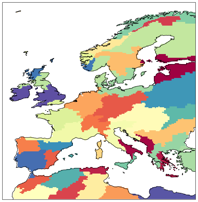
Figure 1 The 38 precipitation regions over which we aggregate precipitation, shown here with arbitrary colouring. Regions were defined through a clustering of 0.25° ERA5-land daily precipitation, as described in Sect. 2.2.

2.3 Precipitation decomposition and flow precursors

To analyse heavy precipitation occurrence we decompose it into dynamical contributions and conversion contributions. The dynamical contribution accounts for the occurrence of different synoptic flow conditions associated with heavy precipitation, based on precursor indices as described below. The conversion contribution accounts for the fine-scale processes that produce precipitation under a given synoptic condition, including microphysics, thermodynamics, boundary layer interactions, the land surface and mesoscale dynamics.

The mathematical formalism behind the decomposition is presented in full in Appendix A. In the main text, each equation is introduced as it becomes relevant alongside a corresponding concrete example so that each term can be linked directly to a meteorological reference. As a matter of notation, probabilities are always marked with a tilde if they correspond to a potentially biased quantity, and with an asterisk if they correspond to a future climate state.

The flow precursor framework developed in Dorrington et al. (2024a), is the basis of our decomposition. On a high level, the approach identifies the synoptic conditions corresponding to past heavy precipitation events using composite analysis, and defines time-evolving “precursor activity indices” based on those composites. While the flow precursor framework can be used for time-lagged dynamical fields, here we only use fields co-occurring with precipitation to form “lag-0 precursors”, but retain the terminology for consistency with (Dorrington et al., 2024a, b). Our method for this paper is as follows:

1. For each region and season, composites of deseasonalised ERA5 Z500, U850 and V850 anomalies are computed for heavy precipitation days. Seasonal cycles are computed with a day-of-year climatology, smoothed with a 31 d Gaussian filter.

2. Composites of each variable are partially masked, retaining only gridpoints where anomalies are (i) statistically significant (p < 0.05), (ii) high amplitude (> 0.25 gridpoint standard deviation), and (iii) spatially coherent (significant, high amplitude anomalies form a connected area of > 5 × 10⁵ km²). These masked composites are termed precursor patterns. This masking is intended to algorithmically imitate the approach a researcher might use to hand-define a variability mode such as the box-based North Atlantic Oscillation (NAO) or El Niño–Southern Oscillation. We maintain the same masking parameters as Dorrington et al. (2024a, b) as they have been shown to produce precursors that can be used to predict daily precipitation in a weather forecast context, which we take as a strong test of their dynamical relevance.

3. Daily ERA5 fields are projected onto these masked precursor patterns and the resulting time series are standardised, producing scalar precursor activity indices. By construction, strong positive projection onto these indices is related to increased occurrence of heavy precipitation.

4. Anomaly fields of Z500, U850 and V850 are computed from climate models using the ERA5 seasonal cycle and mean state, thereby preserving all model bias. Model data was not detrended, with the exception of Z500 data for the SSP3-7.0 runs, where we remove a global thickening trend that is dynamically irrelevant as it has no impact on the geostrophic wind. This was done by computing the ensemble- and area-mean Z500 anomaly over the Euro-Atlantic region [80° W–60° E, 30–90° N], smoothing it with a 21-year time-mean Gaussian filter, and subtracting it from each member.

5. Daily anomaly fields for each ensemble member are projected onto the ERA5 precursor patterns, and scaled with ERA5 standardisation parameters.

In combination with the regional precipitation aggregation described in Sect. 2.2, this process represents the interactions between synoptic dynamics and precipitation in each region as a functional relationship between 4 scalar indices: three precursor indices and one precipitation index. The time evolution of each precursor index is directly interpretable in terms of the evolution of its precursor pattern, just as, for example, the dipole variability of the NAO can be captured neatly within an NAO index. However, in contrast to the NAO, which represents the dominant variability mode of Atlantic geopotential height, the flow precursor framework identifies targeted patterns for each region-season combination that explain heavy precipitation variability. Thus, the framework captures stronger dynamical modulation of precipitation than traditional regime or analogue-based approaches. Figure S2 shows an exemplary comparison for DJF. We discuss only a small number of these precursor patterns explicitly in this paper, but the full set of 3 × 4 × 38 patterns is included in the Supplement and can be visualised at https://uib-precursors-cmip6-interactive.hf.space/app (last access: 15 April 2026) so that specific regional cases can be examined by the interested reader.

2.4 Uncertainty and variability

We quantify both the statistical sampling uncertainty and internal variability of our results. Bias terms for each model are computed using daily output of all ensemble members concatenated. Change terms are computed similarly by comparing the full future and historical ensembles. For both bias and change, sampling uncertainty is computed using 400 bootstrapped resamples of the daily ensemble data with replacement. Internal variability is quantified using the full ensemble spread, with all terms computed for each member separately.

3 Heavy Precipitation in CESM2 and MPI-GE

We first summarise model performance from the bulk perspective with reference to the ERA5-land climatology of 95th percentile regional precipitation (Fig. 2a–d). We term precipitation over this 95th percentile threshold as heavy precipitation, but this should always be understood in local terms. The 95th percentile is highly variable across seasons and regions, ranging from less than 2.5 mm d⁻¹ to as much as 25 mm d⁻¹ (cf. Table S1). Both CESM2 and MPI-GE generally underestimate the intensity of the 95th percentile of precipitation (Fig. 2e–l), especially in summer. Biases are typically largest in mountainous regions, but this is not universally the case: MPI-GE performs well over the Iberian mountains for example, while CESM2 performs well over the Scandinavian mountains. Pronounced wet biases are rare, but can be seen in DJF in some western European regions in both models.

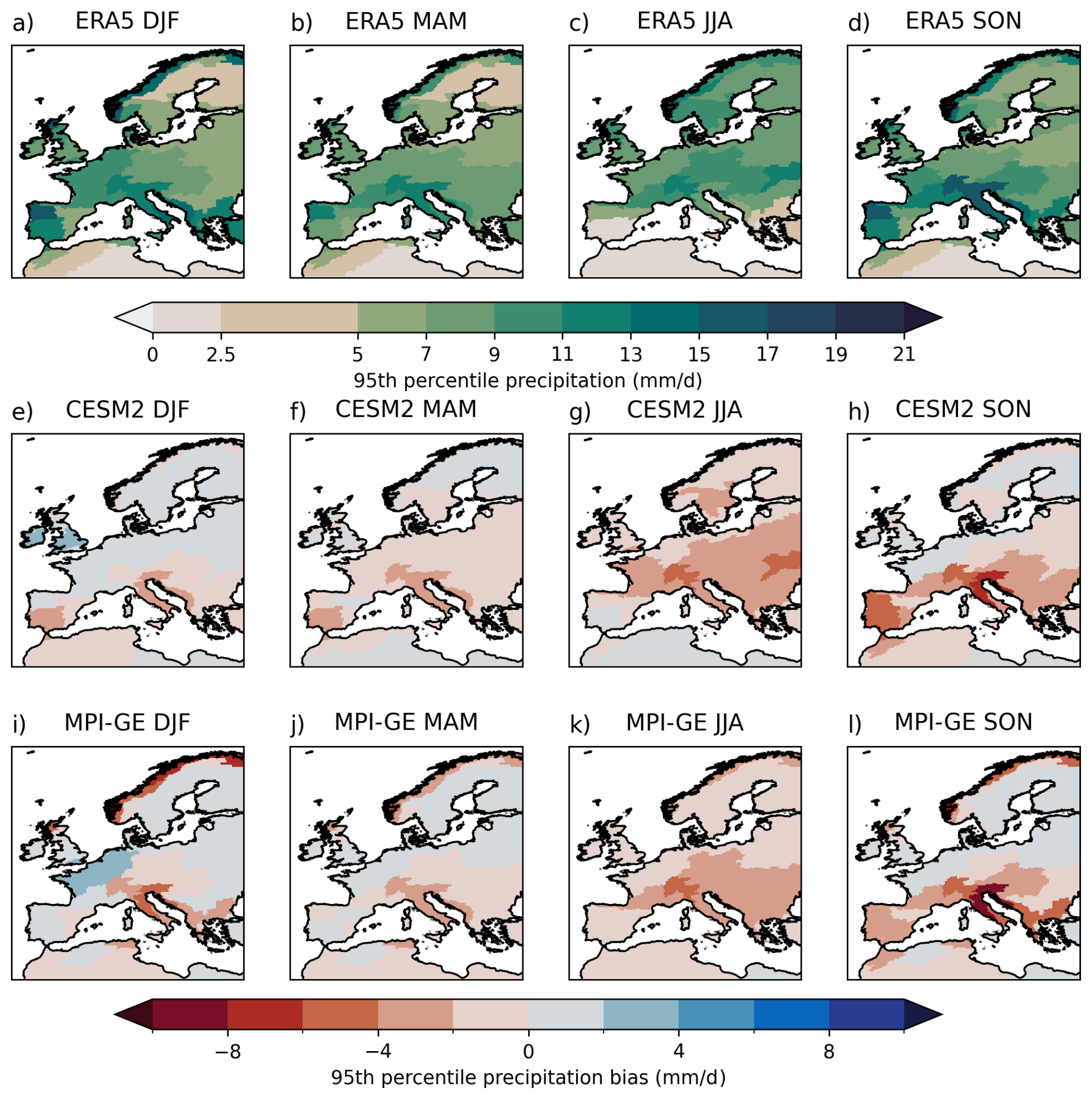
Figure 2 (a–d) 95th percentile area-averaged daily precipitation thresholds from ERA5-land used to define heavy precipitation days. (e–l) Mean biases in 95th percentile precipitation in the two large ensembles.

We focus on the occurrence probability of heavy precipitation (Fig. 3a–h), but there is a strong monotonic relation between deviations in extreme precipitation intensity and occurrence (cf. Fig. S3). Even in regions with the largest magnitude dry biases, such as the Alps or northern Scandinavia (cf. Fig. 2), both models can produce heavy precipitation events of real-world intensity. Nevertheless, occurrence biases worse than −80 % – visible for both models in JJA and for MPI-GE in mountainous domains throughout the year – indicate cases where 95th percentile real-world events are akin to 99th percentile or greater events in the model. Positive occurrence biases are also seen in many regions: the Atlantic coast of Europe in SON and DJF receives 30 %–110 % more heavy precipitation events in the two models than in reality. This motivates our choice to define heavy precipitation events with reference to reanalysis precipitation thresholds, as a pan-European analysis using model-derived thresholds would mix events of differing magnitudes.

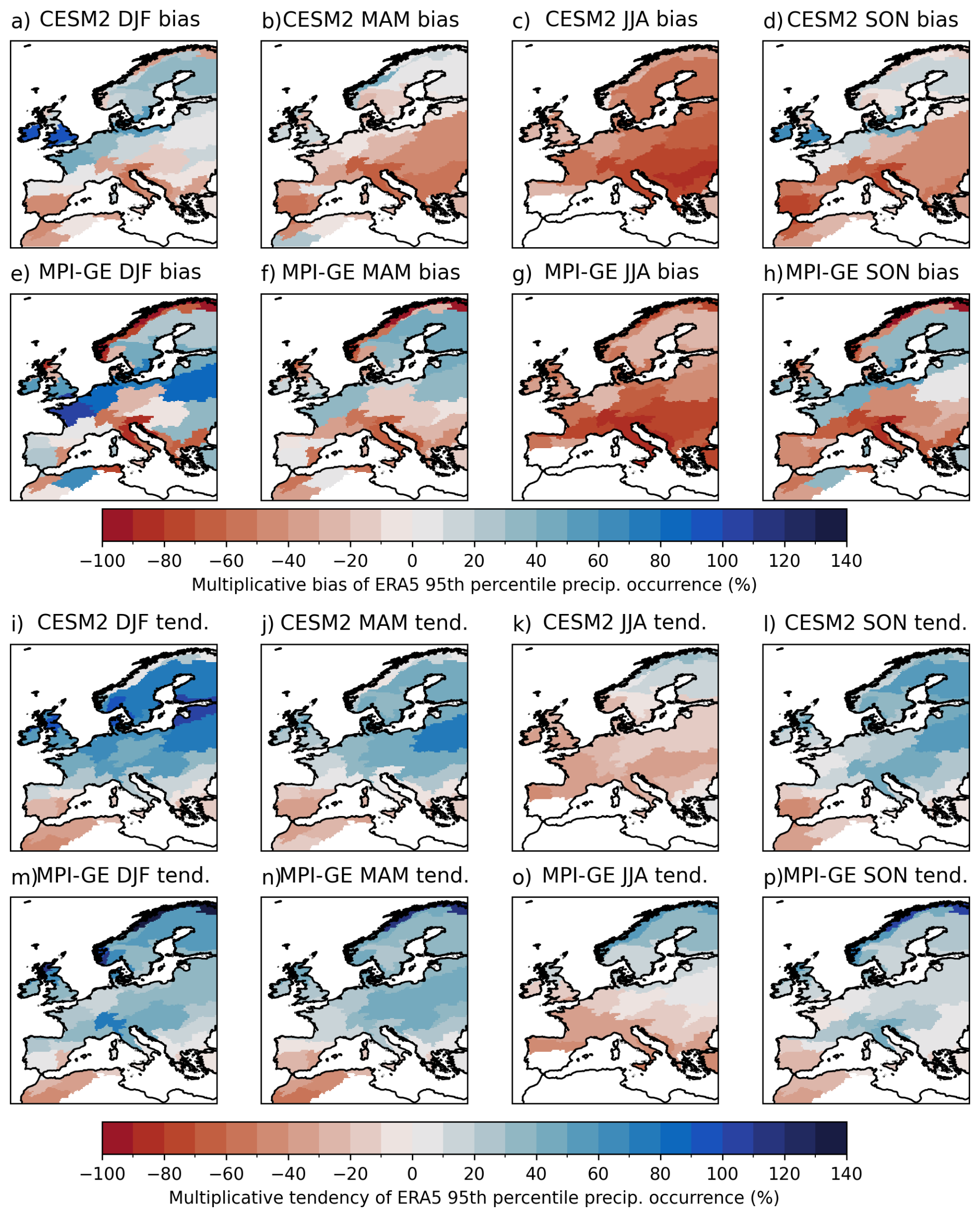
Figure 3 (a–h) Multiplicative biases in the occurrence of heavy precipitation days for each season and model over the historical period (1979–2014), with respect to ERA5-land. (i–p) Ensemble mean multiplicative changes in heavy precipitation occurrence between the future period (2060–2100, SSP3-7.0 scenario) and the historical period. A bias of −100 % would indicate no heavy precipitation occurrence, +100 % would indicate a doubling in occurrence probability with respect to ERA5-land.

Throughout the paper we will characterise forced climate signals as changes in heavy precipitation occurrence between the end-of-century period 2060–2100 under the SSP3-7.0 climate scenario and the historical period 1979–2014. Figure 3i–p shows that these changes are more spatially coherent than the biases, and in general of smaller amplitude. The models show a qualitative consistency in their continental-scale forced response: more heavy precipitation events poleward of 40° N in autumn through spring, fewer events in summer (excluding Fennoscandia) and fewer events in southern Iberia and North Africa throughout the year. This is generally consistent with the “wet gets wetter” heuristic (Held and Soden, 2006). On a region-by-region level, however, and with an eye to the actual amplitude of projected changes, the story is richer and more uncertain. We identify a few specific cases that we will discuss in detail later. CESM2 and MPI-GE have pronounced differences in biases and changes in southwestern Iberia during DJF, which notably is a region where climate models have struggled to reproduce recent observational precipitation trends (Donat et al., 2023). The northern Adriatic region features some of the highest precipitation values in Europe (Fig. 2a–d) and experiences some of the most pronounced societal impacts from flash flooding (e.g. Dorrington et al., 2024b), yet is unfortunately one of the regions where the models we consider show consistent heavy precipitation biases of −60 % to −90 % (Fig. 3a–h). Finally, we note a decrease in JJA heavy precipitation over the central UK and Ireland, which is seemingly consistent across the two models but is shown in Sect. 5 to be a case of considerable model disagreement.

4 Biases

Heavy precipitation occurs when (a) the synoptic environment is favourable and (b) the interactions of sub-synoptic processes serve to convert the large-scale forcing into precipitation. Formalising this observation, we can decompose the daily probability of heavy precipitation, P_H, into the probability of a particular synoptic driver occurring, P_S, and the conditional probability of heavy precipitation under that synoptic driver, P_H|S, summed over a comprehensive set of drivers (indexed by k):

$$P_H=\sum _k{P}_{H|S_k}\cdot P_{S_k}\sum _k{P}_{S_k}=\mathrm{1}$$

The stronger the conditioning of heavy precipitation occurrence on this synoptic categorisation, the more useful this decomposition. Throughout, potentially biased quantities are denoted with a tilde, while future quantities are denoted with an asterisk.

We define our set of synoptic drivers {S_k} using the flow precursor indices introduced in Sect. 2.3. For each region-season combination, precursor patterns are defined using Z500, U850, and V850 anomaly fields (examples for three region-seasons are shown in Fig. 4I–III). Each pattern is used to define a standardised precursor index describing the daily variability of projections onto the pattern. Taking the first principal component of the three ERA5 precursor indices for each region-season produces a single scalar index, S, that captures the variability of multivariate precipitation-causing dynamics. Reducing three precursors to a single index removes information, and principal component analysis cannot account for any nonlinearity in the covariance between precursors. Nevertheless, we use this simplification here to maintain a manageable analytic scope. We next discretise the index S into N bins, $\left\{S_{\mathrm{1}},\mathrm{\dots }{S}_k,\mathrm{\dots }{S}_N\right\}$, representing different synoptic states. In ERA5, each bin is equally likely to occur by construction, and bins labelled with larger k indicate states with a higher conditional probability of heavy precipitation. Using a coarser discretisation can slightly reduce sampling uncertainty (see discussion in the Supplement) while a finer discretisation will more accurately estimate dynamical impacts. We use N = 10, discretising S into deciles.

Using southwestern Iberia during DJF as an example, Fig. 4I shows the identified precursor patterns; the low-level jet is shifted equatorward, and an omega-type block is present over the Atlantic. This pattern favours the convergence of moist Atlantic airmasses from the north and west into the region (as also documented in Dorrington et al., 2024a). Figure S4 shows the precursor patterns for each variable in more detail. The Z500, V850 and U850 precursor indices that summarise the variability of this flow pattern are combined into the multivariate index S, and Fig. 4Ia–d shows ERA5 circulation composites for different deciles of S. High decile composites (k = 9, 10) closely match the precursor pattern, while low deciles (k = 1, 2) show an approximately inverse flow with anticylonic ridging to the west of Iberia and weakened regional westerlies. Figure 4Ie–h confirms that strong precursors correspond to elevated heavy precipitation probability, validated here with a different precipitation dataset than that used to define the patterns – gridpoint-wise heavy precipitation occurrence computed from MSWEP data.

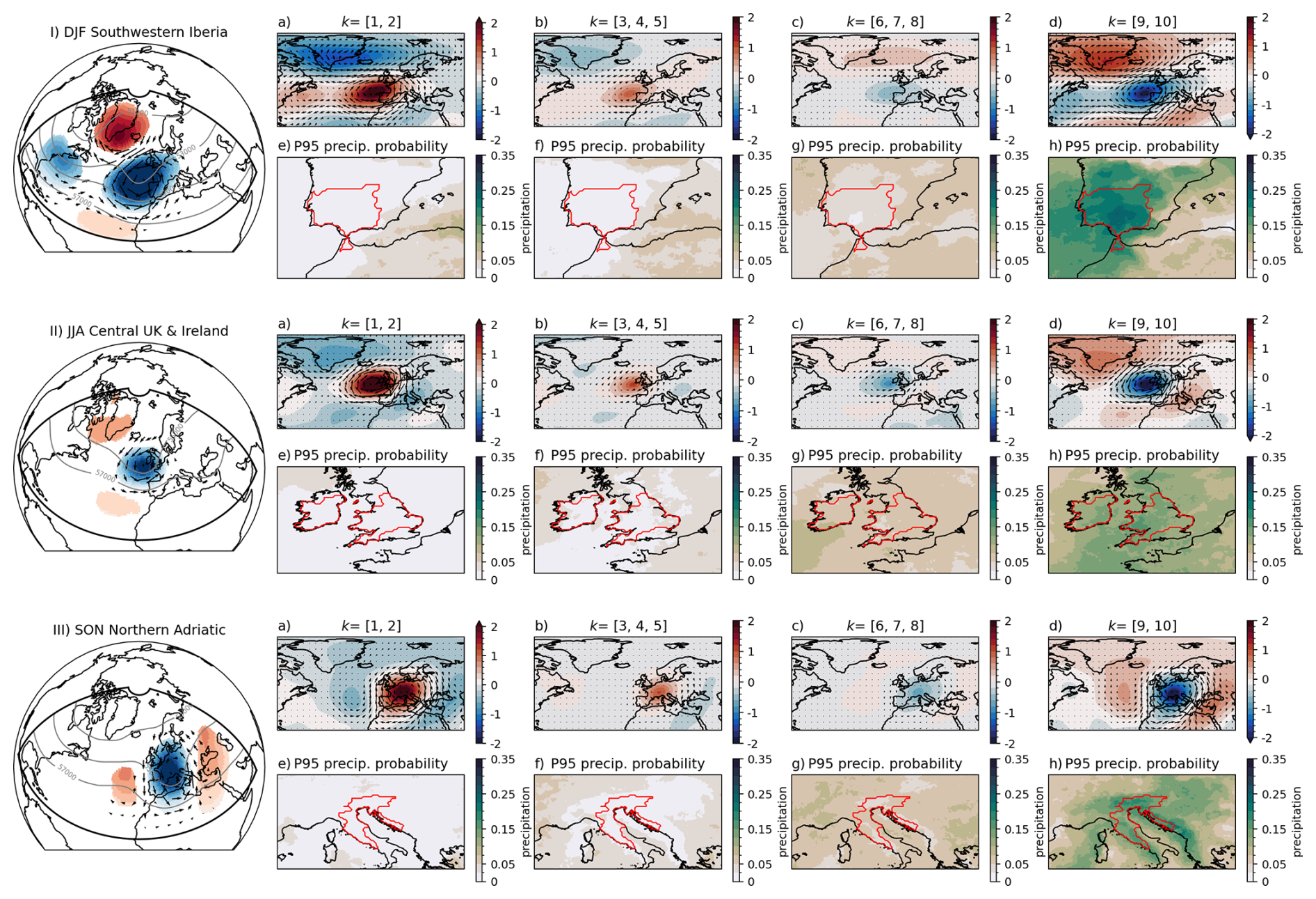
Figure 4 Precursor patterns (I)–(III) and circulation composites on bins of the synoptic index S_k (a–d) for three example region-seasons. In all panels, blue-red shading shows standardised anomalies of ERA5 500 hPa geopotential height, and black arrows indicate ERA5 850 hPa wind. Grey contours on the left panels (I)–(III) show full geopotential height contours associated with the precursor patterns. Strong precursors lead to increased heavy precipitation probability (e–h), where white-to-green shading shows gridpoint 95th percentile precipitation probability from MSWEP data. Red contours, show the domains over which precipitation is spatially aggregated.

In a historical model simulation with heavy precipitation probability ${\stackrel{\mathrm{̃}}{P}}_H$, we decompose biases into additive bias in the occurrence frequency of different synoptic conditions, $\mathit{\delta }{P}_{S_k}$, and multiplicative biases in the probability of heavy precipitation conversion for each synoptic condition, ξ_k. Formulating the conversion bias as multiplicative follows standard precipitation calibration methods (Hewson and Pillosu, 2021). Our decomposition of model heavy precipitation occurrence is then:

$$\begin{array}{}\text{(1)}& {\stackrel{\mathrm{̃}}{P}}_H=\sum _k\left(P_{H|S_k}\left[\mathrm{1}+{\mathit{\xi }}_k\right]\right)\cdot \left(P_{S_k}+\mathit{\delta }{P}_{S_k}\right)\end{array}$$

Instead of having a single bulk metric of precipitation bias for each region and season, we now have 20 metrics ($\mathit{\delta }{P}_{S_k}$ and ξ_k for ten values of k), representing biases on different scales and in different flow states. As a note, previous literature (e.g. Deser et al., 2016; Pfahl et al., 2017; Doane-Solomon et al., 2025; Fischer et al., 2025) has often labelled similar quantities to our conversion term as an “intensity” or “thermodynamic” term. The former is a better descriptor for continuous precipitation than for our categorical perspective, while we avoid the latter due to the many non-thermodynamic factors it can include, as noted in Sect. 2.3.

4.1 Wintertime biases in southwestern Iberia

Figure 5 visualises the decomposed terms of Eq. (1) for DJF southwestern Iberia in CESM2 and MPI-GE. In this case, both models have large and opposite dynamical biases (Fig. 5a): CESM2 generates too few days with strong precursors (i.e. $\mathit{\delta }{P}_{S_{\mathit{\{}\mathrm{8},\mathrm{9},\mathrm{10}\mathit{\}}}}$ < 0) while MPI-GE generates far too many, producing flows like Fig. 4Id almost a third of the time. The conversion terms from ERA5 clearly show that strong synoptic precursors (k = 10) are almost a prerequisite for heavy precipitation (Fig. 5b). CESM2 simulates the occurrence of heavy precipitation relatively well for moderately strong precursors (6 < k ≤ 9), with some underestimation for the strongest 10 % of flows, whereas MPI-GE exhibits markedly low heavy precipitation conversion for all of the strongest 40 % of precursor flows.

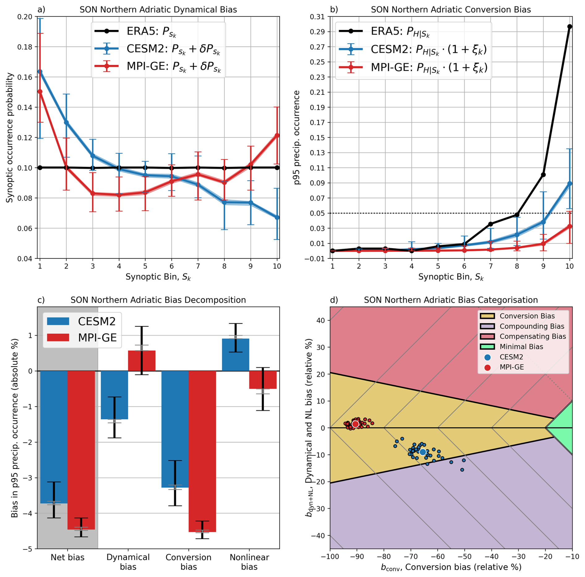
Figure 5 Flow-dependent precipitation bias for southwestern Iberia during DJF. (a) Occurrence of different bins of the synoptic index over the historical period. Differences between model (red,blue) and ERA5 reference values (black) determine the dynamical bias. (b) Heavy precipitation occurrence conditional on synoptic index bin. Dashed black line shows the 5 % climatological heavy precipitation rate Differences between model (red,blue) and ERA5 reference values (black) determine the conversion bias. (c) Decomposition of net heavy precipitation biases into contributions from dynamical and conversion terms and their non-linear interaction. (d) A visualisation of model bias in the 2-dimensional (2D) space of conversion bias and summed dynamical and non-linear bias. Individual ensemble members are shown with black outlines, ensemble mean values with white outlines. The dashed negative diagonal marks the line of zero net bias. Grey diamonds mark contours of constant absolute bias. The significance of the shaded regions is explained in the main text. The 95th percentile sampling uncertainty estimate is shown with shading in panels (a) and (b), grey bars in panel (c) and is smaller than the ensemble mean dot in panel (d). The full spread of internal variability is shown in bars in panels (a) and (b), black bars in panel (c) and visualised directly in panel (d).

These flow-dependent biases can be aggregated into a three-term bias budget:

$$\begin{array}{}\text{(2)}& \begin{array}{rl}& \text{model bias}={\stackrel{\mathrm{̃}}{P}}_H-P_H\\ & =\sum _k{P}_{H|S_k}\left(\underset{\text{conversion bias}}{\underbrace{{\mathit{\xi }}_k{P}_{S_k}}}+\underset{\text{dynamical bias}}{\underbrace{\mathit{\delta }{P}_{S_k}}}+\underset{\text{non-linear bias}}{\underbrace{{\mathit{\xi }}_k\cdot \mathit{\delta }{P}_{S_k}}}\right)\end{array}\end{array}$$

These terms are shown in Fig. 5c, with the amplitudes of each term directly interpretable in units of altered heavy precipitation occurrence. CESM2 both undersamples strong precursor circulations (negative dynamical bias) and underestimates the conversion of strong precursors into heavy precipitation (negative conversion bias). The resulting dynamical and conversion biases compound, leading to a net bias of −2 %; heavy precipitation in the region only occurs 3 % of the time in CESM2 versus 5 % in ERA5. MPI-GE appears to perform better with a net bias of 1 %, but this is a misleading result that occurs due to compensation between dynamical and conversion biases. The positive dynamical bias of MPI-GE would imply a heavy precipitation occurrence of 8.5 %, but the model's severe under-conversion of dynamical forcing into heavy precipitation reduces this substantially. The two models' biases in this case are then not only of opposing sign, but of opposing type – compensating in MPI-GE and compounding in CESM2.

Different types of bias have different implications for model usability and interpretation. We propose five conceptual categories of bias which we discuss in detail in Sect. 7. To do this, we define a 2D bias space consisting of the conversion term, b_conv, and the sum of the dynamical and non-linear terms¹ b_dyn+NL, with an L1-norm b = $\left|b_{\text{conv}}\right|+\left|b_{\mathrm{dyn}+\mathrm{NL}}\right|$ where b is the absolute bias. Figure 5d shows the southwestern Iberia biases within this space and visualises internal variability within the ensembles. Within this space we define five categories of bias, where we introduce two parameters, b_max (a maximum “acceptable” bias level) and R (a relative importance threshold for different terms):

1. Minimal bias: $b\le b_{max}$

2. Conversion bias: $\frac{\left|b_{\mathrm{dyn}+\mathrm{NL}}\right|}{\left|b_{\mathrm{conv}}\right|}\le R$ and $b>b_{max}$

3. Dynamical bias: $\frac{\left|b_{\text{dyn+NL}}\right|}{\left|b_{\mathrm{conv}}\right|}\ge \frac{\mathrm{1}}{R}$ and $b>b_{max}$

4. Compounding bias: sign(b_conv) = sign(b_therm) and bias not Minimal/Conversion/Dynamical

5. Compensating bias: sign(b_conv) ≠ sign(b_therm) and bias not Minimal/Conversion/Dynamical

We set b_max = 20 % and R = 0.2 to provide a proof-of-concept, but we stress that these should be tuned for user needs. For MPI-GE, variability in b_conv is small and independent from the bias in b_dyn+NL, which ranges from 20 %–80 %. Notably, several ensemble members lie close to the line of zero net bias (marked by the dashed diagonal) while lying on the b = 80 % contour. In contrast, the CESM2 ensemble members are closely clustered around the b = 40 % contour, all with similar net bias and showing strong intra-ensemble correlation between b_conv and b_dyn+NL. The CESM2 spread contains both members for which bias is almost entirely dynamical and those for which bias is predominately conversion-related, highlighting the importance of large ensembles to understand model bias in detail.

4.2 Autumn biases in the northern Adriatic

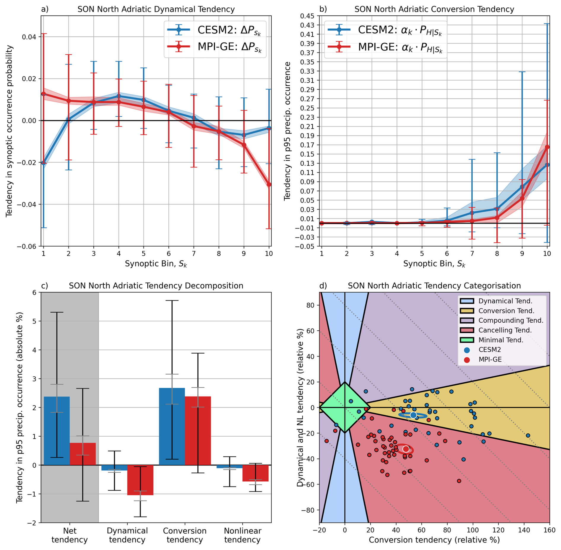
The northern Adriatic in SON provides a second example with very different bias features. In this case heavy precipitation is not predominately driven by large-scale blocks or jet anomalies but by Rossby wave packets of zonal wavenumbers 6–7 (Grazzini et al., 2021), visible in the precursor patterns and synoptic composites of Fig. 4IIIa–h. Figure 6a reveals moderate dynamical biases: MPI-GE favours strong wave-trains in phases that both favour (k = 10) and suppress (k = 1) precipitation, while CESM2's bias towards negative precursors indicates a persistent Autumn ridge over central Europe (cf. Fig. 4IIIa). However these dynamical biases are minor overall in comparison to the conversion biases shown in Fig. 6b. Both models have severe challenges converting dynamical drivers into precipitation, a conversion which in the real world relies on factors these models cannot resolve: convection, diabatic processes over the warm, shallow Adriatic, and uplift and blocking from the Apennines and the Alps. As a result, conversion dominates the bias budget for both models and non-linear terms almost completely cancel the dynamical bias (Fig. 6c–d), representing that biases in rainfall-favouring dynamics are of little importance if a model would very rarely produce heavy rain anyway. In Sect. 6 we will discuss how usable information about future heavy precipitation can be obtained from models even in such cases of severe historical bias.

Figure 6 As in Fig. 5 but for the northern Adriatic region in SON.

4.3 Biases across Europe

We now take a holistic view of model biases, considering each season and region, excepting extremely dry cases where the ERA5 heavy precipitation threshold is less than 2.5 mm. Figure 7 shows the impact of conversion biases to heavy precipitation, as given by Eq. (2). The most coherent feature is the systematic under-estimation of JJA heavy precipitation conversion in both models, with occurrence biases of −60 % to −80 %. Similar, although typically weaker, conversion biases are seen in MAM and SON for central and southern Europe. Many of these cases correspond to wave-driven flows similar to the SON North Adriatic case or Mediterranean cutoff lows (see supplementary material), and it is plausible this low conversion captures poorly represented diabatic, convective and orographic processes.

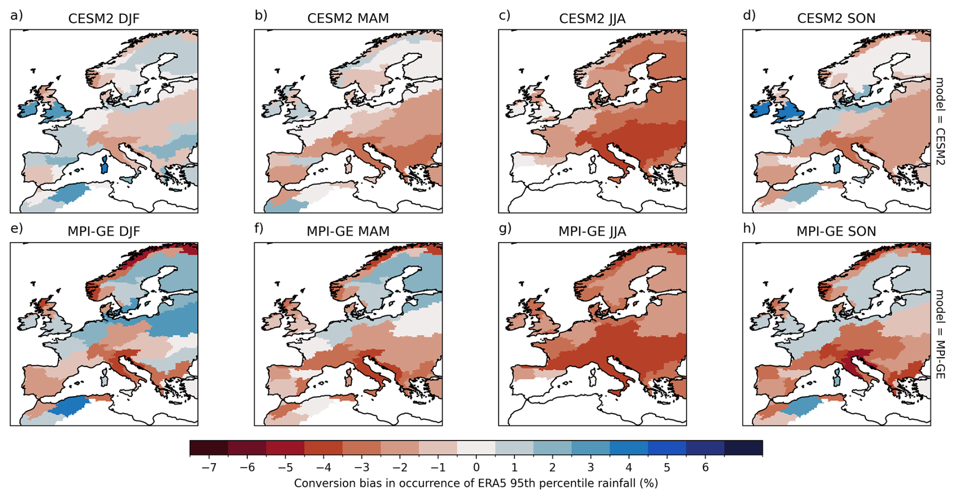
Figure 7 Ensemble mean biases in heavy precipitation occurrence attributable to conversion biases (errors in the conversion of synoptic forcing into heavy precipitation). Results are not shown for region-seasons where the heavy precipitation threshold ≤ 2.5 mm d⁻¹.

In contrast, conversion biases in Northern Europe during MAM and SON can be positive, primarily in cases where large-scale zonal flows with fast eastward-extended jets form the main rainfall precursor. Conversion biases are most spatially diverse in DJF, perhaps surprisingly given the larger scale synoptic organisation. MPI-GE in particular struggles to convert dynamical precursors to heavy precipitation in the most mountainous domains. Regional downscaling over Norway increases DJF precipitation from convective sources and localises it on the coast (Iversen et al., 2023), suggesting that resolution (possibly compounded by snow parameterisation errors) is likely the cause of these conversion biases.

Dynamical contributions to heavy precipitation bias are in general more spatially coherent than the conversion biases but are very different between the two models (Fig. 8), and are partly linked to jet stream biases. CESM2 has positive dynamical biases in wintertime heavy precipitation over northern Europe (Fig. 8a) due to an overly strong and eastward extended jet (Simpson et al., 2020), with negative dynamical biases over southern Europe due to a corresponding lack of wave-driven and negative NAO-like flows. Through the rest of the year, CESM2 shows dry biases in western Europe (Fig. 8b–d) due to a mispositioned jet and a persistent Atlantic ridge anomaly. MPI-GE has a very different dynamical bias pattern, with precipitation-causing weather patterns occurring excessively throughout SON, DJF and MAM. This is a signature of excessive wave activity and wintertime cutoff-lows in the East Atlantic, the latter of which may be related to MPI-ESM-LE's overly southward and zonal jet stream (Simpson et al., 2020). This wet dynamical bias in MPI-GE is consistent with the “overshooting” precipitation found in higher resolution MPI-ESM models (Olonscheck et al., 2023), since resolution increases may disproportionately reduce the model's negative conversion biases while leaving the positive dynamical bias relatively unchanged.

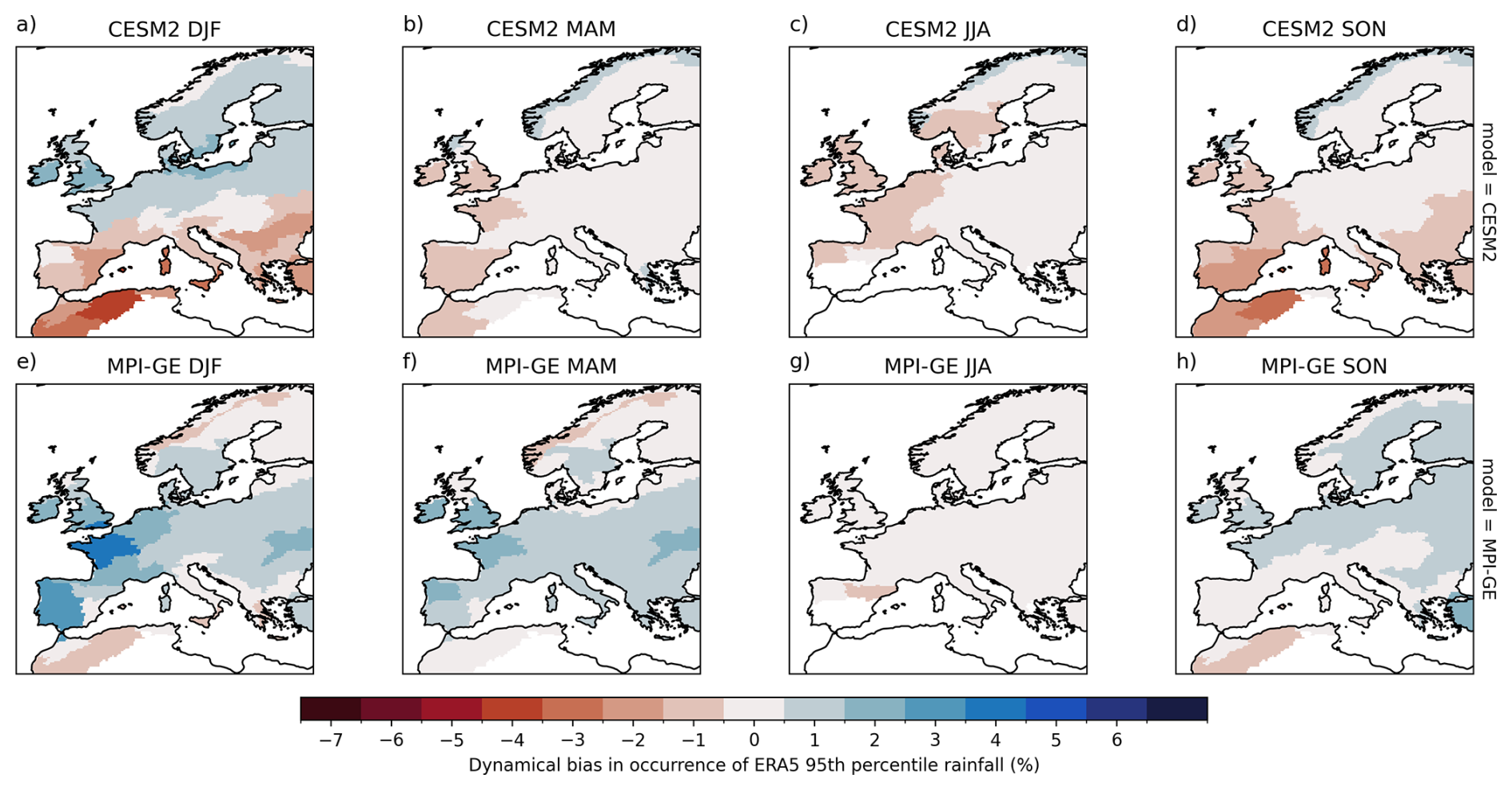
Figure 8 Ensemble mean biases in heavy precipitation occurrence attributable to dynamical biases (errors in the distribution of synoptic weather patterns). Results are not shown for region-seasons where the heavy precipitation threshold ≤ 2.5 mm d⁻¹.

Figure 9 synthesises these biases using the 5-category bias categorisation introduced in Sect. 4.1. Results for all seasons and regions are also visualised in bias-space in Fig. S5, offering an alternate perspective. Firstly, we note that achieving minimal bias is possible for both models in some regions, even if fairly uncommon – the daily, regional, and near-extreme scales we are interested in are not inherently beyond the capabilities of CMIP6-class models. Secondly, we see that conversion biases are common, especially in JJA, as expected due to the relevance of summertime convection, and yet dominant dynamical biases can occur in any seasons. Perhaps most importantly, we emphasise that compensating biases – as we identified for MPI-GE during DJF over South West Iberia – are common, occurring in both models throughout the year. The two models tend to favour compensating biases of particular sign: CESM2 features excessive conversion for too-rare synoptic conditions, while MPI-GE counterbalances too-common synoptic conditions with weak conversion (cf. Fig. S5).

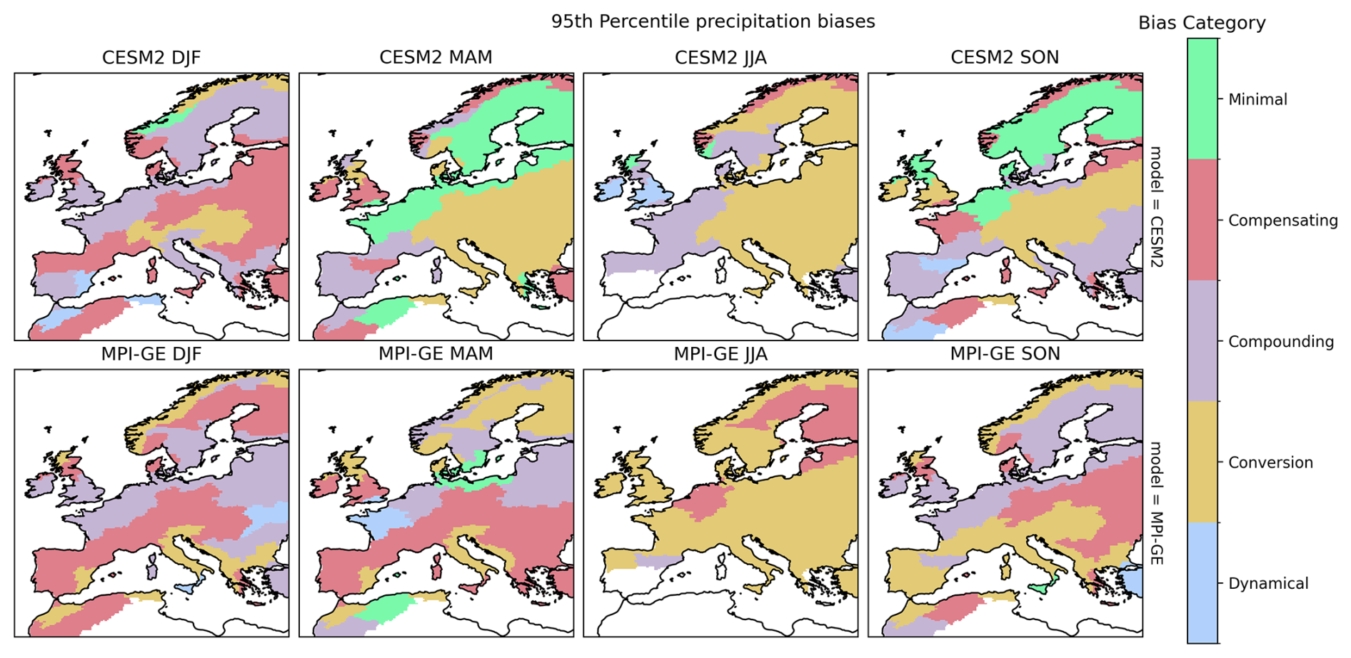
Figure 9 Categorisation of model biases based on the relative contribution of their conversion and dynamical biases. See main text for details.

5 Forced Changes

We now turn to future projections, considering the change in heavy precipitation occurrence between 2060–2100 under the SSP3-7.0 scenario and the historical period 1979–2015. We focus on the change, rather than a trend with respect to global temperature, to avoid conflating global and local changes. In Sect. 4 we demonstrated that both models contain pronounced heavy precipitation biases for certain regions, coming from errors in both the driving synoptic dynamics and the regional processes that convert those dynamics into heavy precipitation. When considering forced changes can these biases be ignored, or do they distort the projected forced response or even completely undermine the model's utility?

We first consider an estimate where we assume biases have no impact on forced changes. This is the perspective used, often implicitly, when directly computing the bulk relative change in model precipitation, which we denote $\stackrel{\mathrm{̃}}{\mathit{\beta }}$, from the model's heavy precipitation occurrence in the future, ${\stackrel{\mathrm{̃}}{P}}_H^{*}$, and in the historical period, ${\stackrel{\mathrm{̃}}{P}}_H$:

$$\begin{array}{}\text{(3)}& {\stackrel{\mathrm{̃}}{P}}_H^{*}={\stackrel{\mathrm{̃}}{P}}_H\cdot (\mathrm{1}+\stackrel{\mathrm{̃}}{\mathit{\beta }})\end{array}$$

$$\stackrel{\mathrm{̃}}{\mathit{\beta }}={\stackrel{\mathrm{̃}}{P}}_H^{*}/{\stackrel{\mathrm{̃}}{P}}_H-\mathrm{1}$$

Extending Eq. (1) to include forced changes reveals that the bulk estimate of change $\stackrel{\mathrm{̃}}{\mathit{\beta }}$ can in principle be distorted by flow-dependent model biases. In the same way that we decomposed biases in Sect. 4, we consider the dynamical change in the occurrence of each synoptic category, $\mathrm{\Delta }{P}_{S_k}$, and the change in heavy precipitation conversion, α_k, within each synoptic category, which gives:

$$\begin{array}{}\text{(4)}& {\stackrel{\mathrm{̃}}{P}}_H^{*}=\sum _k\left(P_{H|S_k}\left[\mathrm{1}+{\mathit{\xi }}_k\right]\left[\mathrm{1}+{\mathit{\alpha }}_k\right]\right)\cdot \left(P_{S_k}+\mathit{\delta }{P}_{S_k}+\mathrm{\Delta }{P}_{S_k}\right)\end{array}$$

Within Eq. (4) are products between flow-dependent forced changes and flow-dependent biases, which can be thought of as either non-stationary biases or spurious forced signals. As Eq. (4) is the numerator of $\stackrel{\mathrm{̃}}{\mathit{\beta }}$, these distortions also impact the bulk estimate of forced precipitation changes. We quantify the impact of this distortion in Sect. 6. However, if we accept the flow-dependent forced changes as credible estimates of true climate response and if we have no prior reason to expect a model's flow dependent biases to be non-stationary, then as part of our decomposition we can drop these bias-change cross terms. We then obtain a calibrated estimate of the overall heavy precipitation change, β:

$$\begin{array}{}\text{(5)}& \text{Forced change}=P_H\cdot (\mathrm{1}+\mathit{\beta })\end{array}$$

$$\mathit{\beta }={\displaystyle \frac{\mathrm{1}}{P_H}}\sum _k{P}_{H|S_k}\left(\underset{\text{conversion change}}{\underbrace{{\mathit{\alpha }}_k\cdot P_{S_k}}}+\underset{\text{dynamical change}}{\underbrace{\mathrm{\Delta }{P}_{S_k}}}+\underset{\text{non-linear change}}{\underbrace{{\mathit{\alpha }}_k\cdot \mathrm{\Delta }{P}_{S_k}}}\right)$$

When analysing forced changes below, we use this calibrated estimate, but the effect of this calibration should not be overstated. The models' estimates of the flow-dependent forced changes α_k and $\mathrm{\Delta }{P}_{S_k}$ may still ultimately be incorrect – and indeed given disagreements between models, most must be. However these corrected forced changes are at least physically consistent with synoptic dynamics and their link to precipitation in the current observed climate. As a note, a direct computation of α_k = $\frac{{\stackrel{\mathrm{̃}}{P}}_{H|S_k}^{*}}{{\stackrel{\mathrm{̃}}{P}}_{H|S_k}}-\mathrm{1}$ can provide unphysical changes if the historical flow-dependent precipitation probability, ${\stackrel{\mathrm{̃}}{P}}_{H|S_k}$ is very close to zero (see Sect. A4). In these cases, we can reformulate the conversion change as additive by redefining α_k = $\frac{{\stackrel{\mathrm{̃}}{P}}_{H|S_k}^{*}-{\stackrel{\mathrm{̃}}{P}}_{H|S_k}}{P_{H|S_k}}$, but such strongly biased cases will mostly be excluded from discussion unless explicitly indicated.

5.1 Summertime forced changes in the central UK and Ireland

Decomposed precipitation changes can offer new insights into future scenarios, reveal sources of model disagreement, and uncover cases where model disagreement is greater than it initially appears. A good example of hidden model disagreement is given by JJA forced changes over Central UK and Ireland (Fig. 10). Current large-scale summertime heavy precipitation in this region is driven by strong, localised cyclones (cf. Fig. 4II), and is dynamically suppressed by anticyclonic ridges over the east Atlantic (Fig. 4IIa, b, e, f).

Both climate models project a similar net decrease in heavy precipitation: a shift from 5 % to 4 % occurrence probability in CESM2, and to 4.5 % in MPI-GE. However, Fig. 10c shows that the decomposed budget of these forced changes is very different. MPI-GE's forced change is dominated by a negative dynamical contribution (Fig. 10a). CESM2's forced change by contrast is dominated by a negative conversion contribution (Fig. 10b). These are very different scenarios with differing implications: CESM2 describes a world with a similar number of strong summertime cyclones to today, but each less likely to cause heavy precipitation. MPI-GE describes a world with far fewer cyclonic anomalies but each more likely to produce heavy precipitation than those of today. Arguably the smaller net change in MPI-GE corresponds to the more volatile and impactful case.

Just as for biases in Sect. 4.1, we can construct a 2D space of conversion changes and summed dynamical and non-linear changes to define heuristic categories of forced changes. Figure 10d shows this change space, and highlights how ensemble mean signals from both models lie close to the same line of −20 % relative net change (dashed black line), therefore appearing in agreement on a statistically robust decrease in heavy precipitation events from a bulk perspective. However, Fig. 10c–d also demonstrates large internal variability in regional heavy precipitation changes: for any single 40-year period it is not a given that a decrease in heavy precipitation will be observed. The actual real-world implications of this are unclear as climate models have both insufficient low-frequency variability (Mann et al., 2020), including in European circulation features (Dorrington et al., 2022), and also suffer from a signal-to-noise problem which may lead to an overly-weak forced responses (Scaife and Smith, 2018). Regardless, this example also demonstrates how decomposition of changes can help identify signals on which models are confident: while the MPI-GE absolute net change in individual members spans from −1.7 % to 1.5 %, the dynamical change is confidently negative for each member, −1.5 % to −0.3 %.

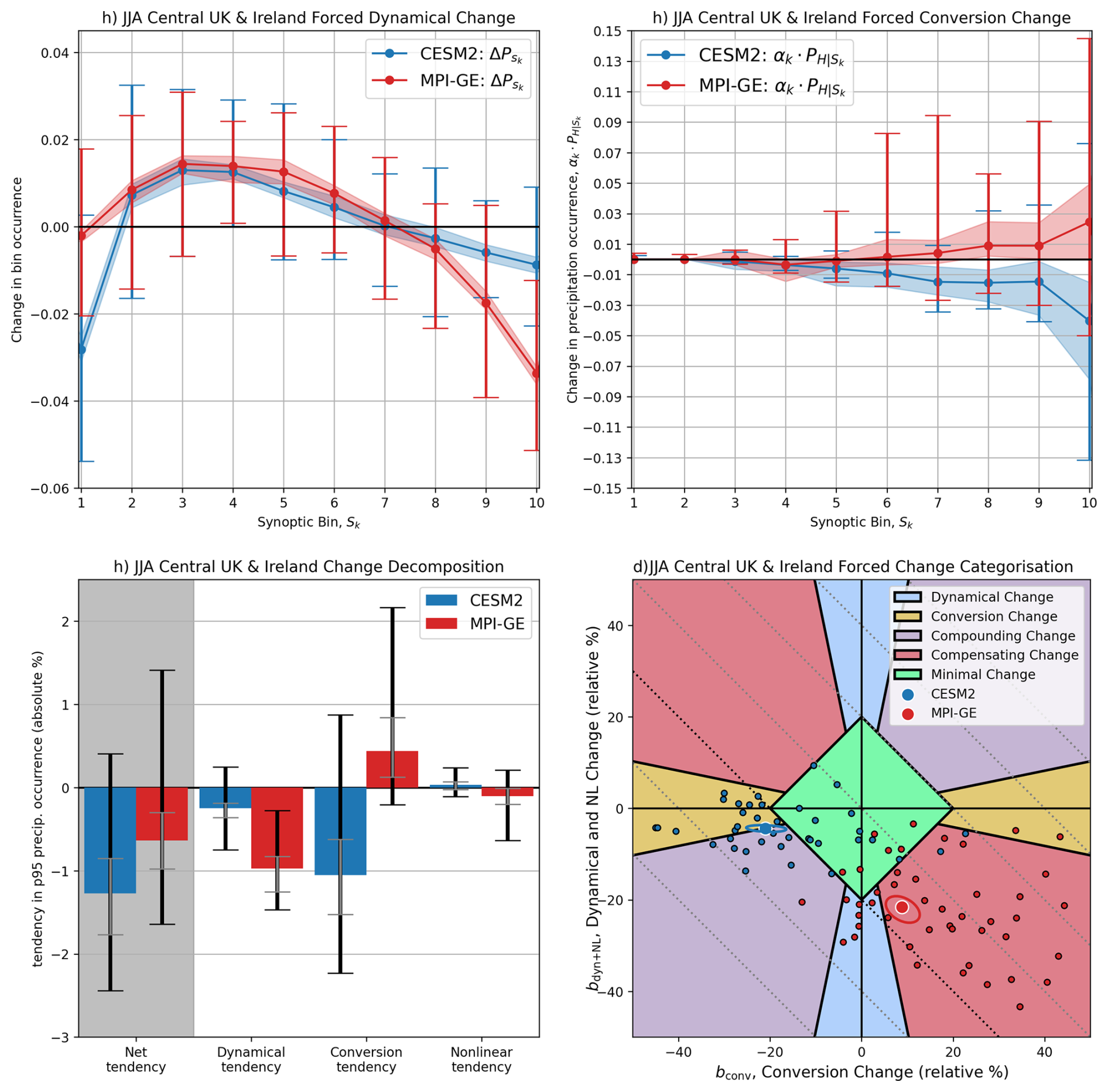
Figure 10 Flow-dependent forced changes in precipitation for the central UK and Ireland during JJA. (a) Changes in occurrence of different bins of the synoptic index, determining the dynamical change. (b) Changes in heavy precipitation occurrence conditional on synoptic index bin, determining the conversion change. (c) Decomposition of net heavy precipitation changes into contributions from dynamical and conversion terms and their non-linear interaction. (d) A visualisation of model forced change in the 2D space of conversion changes and summed dynamical and non-linear changes. Individual ensemble members are shown with black outlines, ensemble mean values with white outlines. Ellipses show the 2-standard deviation confidence interval around ensemble mean changes. Dashed lines mark contours of constant net change, with the −20 % net change shown in bold. The 95th percentile sampling uncertainty estimate is shown with shading in panels (a) and (b) and with grey bars in panel (c). The full spread of internal variability is shown with bars in panels (a) and (b), black bars in panel (c) and visualised directly in panel (d).

5.2 Forced changes across Europe

Figures 11 and 12 show the model conversion, and dynamical changes, respectively. Non-linear changes are small, as shown in Fig. S6. As our decomposition is based on the dominant precipitation driver in observations, it is conceivable that dynamical changes could be misattributed to the conversion term if new dynamics become important drivers of heavy precipitation in the future. Figures S7 and S8 indicate little evidence for this, with future conversion changes driven almost exclusively by changes in conversion during strong precursor situations (k = $[\mathrm{8},\mathrm{9},\mathrm{10}]$).

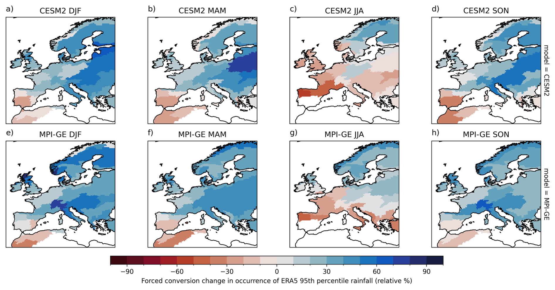
Figure 11 Ensemble mean relative changes (2060–2100, SSP3-7.0) in heavy precipitation occurrence attributable to changes in precipitation conversion. Results are not shown for region-seasons where the historical heavy precipitation threshold ≤ 2.5 mm d⁻¹.

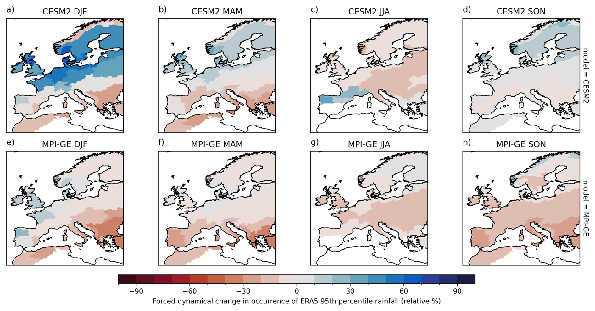
Figure 12 Ensemble mean relative changes (2060–2100, SSP3-7.0) in p95 heavy precipitation occurrence attributable to changes in synoptic dynamics. Results are not shown for region-seasons where the historical heavy precipitation threshold ≤ 2.5 mm d⁻¹.

Bulk forced changes, shown in Fig. 3, indicate a qualitative agreement between CESM2 and MPI-GE on future heavy precipitation occurrence. Broadly speaking, both models project a near zonally symmetric pattern of changes, with an increase in heavy precipitation in northern regions and a decrease in southern regions. The latitude at which the forced change reverses varies between seasons: decreased heavy precipitation below ≈ 55° N in JJA and 40° N in DJF for example. However, decomposing the sources of those changes reveals greater spatial asymmetry and considerable differences between the models.

In wintertime, conversion-driven increases in heavy precipitation occurrence of approx. 40 % occur in both models across all regions outside southwestern Europe (Fig. 11a, e). Notably, this includes the southeastern regions, where strong, negative dynamical changes drive decreased heavy precipitation overall (Fig. 12a, e). This implies a decline of eastern Mediterranean winter cyclones, each individually more likely to cause heavy precipitation but leading to a net negative change overall. This is consistent with CMIP6 results from a cyclone-focused analysis (Chericoni et al., 2025), although they found the forced signal changed dramatic dramatically in higher resolution simulations.

In northern Europe, the models disagree on sign and amplitude of dynamically-driven changes, with little signal in MPI-GE and 50 %–90 % increases in heavy precipitation in CESM2, caused by more frequent and stronger eastward jet extensions. CESM2's negative dynamical changes along the north Norwegian coast may be linked to the model's pronounced North Atlantic warming hole (Iversen et al., 2023) and the decline of cold-air outbreaks into the Greenland Sea (Konstali et al., 2024). In MAM and SON, MPI-GE predicts a decline in heavy precipitation over southwestern regions due to compounding conversion and dynamical changes (Figs. 12 and 11f, h). In JJA, MPI-GE shows negative conversion changes in much of west and south-east Europe (Fig. 11e). CESM2 has similar conversion changes to MPI-GE (Fig. 11b–d), but different dynamical changes. CESM2 shows positive dynamical changes in MAM and SON in Northern Europe (Fig. 12b–d) again related to a projected eastward jet extension, while negative dynamical changes in JJA relate to a projected less wavy summertime-flow (the reliability of which remains contentious; Stendel et al., 2021). It has recently been suggested that JJA extreme precipitation may be “shifting” to MAM and SON (Zhu et al., 2025), as summer rainfall decreases and shoulder season rainfall increases, consistent with Fig. 3. We see here that this is not a coherent phenomena, but rather is dynamically driven in some regions and seasons, and driven by local-scale conversion changes in others.

The differences across space and between the two models are highlighted through the categorisation of heavy precipitation changes shown in Fig. 13 (and also in a 2D-space in Fig. S8). Predominately dynamical changes are rare, while changes in the relationship between synoptic dynamics and the surface (that is, a change in conversion) are nearly ubiquitous. However, dynamical changes cannot be neglected, as the majority of cases feature compensating and compounding changes where dynamical and conversion contributions are of similar magnitude.

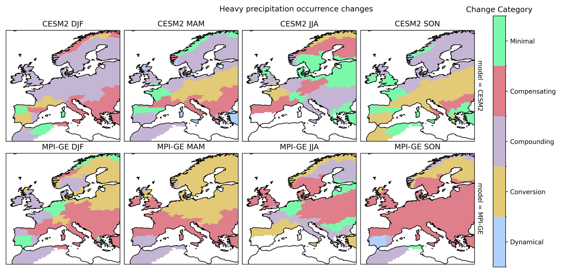
Figure 13 Categorisation of ensemble mean model changes based on the relative amplitude of their conversion and dynamical changes. See main text for details.

6 Bias-Change Interactions

In the previous section, we showed that the calibrated heavy precipitation changes computed from Eq. (5) are not equivalent to the bulk change that would be given by Eq. (3): we neglected terms that represent the interactions of flow dependent biases with flow dependent forced changes. How important is this difference in practice? Because Eqs. (4) and (3) have different denominators, the cross-terms alone do not explain the difference between bulk and flow-corrected changes. Instead the difference between bulk ($\stackrel{\mathrm{̃}}{\mathit{\beta }}$) and flow-corrected (β) multiplicative changes is given by (see Appendix A for derivation):

$$\begin{array}{}\text{(6)}& \stackrel{\mathrm{̃}}{\mathit{\beta }}-\mathit{\beta }=\sum _k({\mathit{\alpha }}_k\cdot \left[{\stackrel{\mathrm{̃}}{F}}_k-F_k\right]+(\mathrm{1}+{\mathit{\alpha }}_k)\cdot \mathrm{\Delta }{P}_{S_k}\cdot \left[{\stackrel{\mathrm{̃}}{G}}_k-G_k\right]),\end{array}$$

where:

$$\begin{array}{rl}& F_k={\displaystyle \frac{P_{H|S_k}\cdot P_{S_k}}{P_H}}=P_{S_k|H}{\stackrel{\mathrm{̃}}{F}}_k={\displaystyle \frac{{\stackrel{\mathrm{̃}}{P}}_{H|S_k}\cdot {\stackrel{\mathrm{̃}}{P}}_{S_k}}{{\stackrel{\mathrm{̃}}{P}}_H}}={\stackrel{\mathrm{̃}}{P}}_{S_k|H}\\ & G_k={\displaystyle \frac{P_{H|S_k}}{P_H}}={\displaystyle \frac{P_{S_k|H}}{P_{S_k}}}{\stackrel{\mathrm{̃}}{G}}_k={\displaystyle \frac{{\stackrel{\mathrm{̃}}{P}}_{H|S_k}}{{\stackrel{\mathrm{̃}}{P}}_H}}={\displaystyle \frac{{\stackrel{\mathrm{̃}}{P}}_{S_k|H}}{{\stackrel{\mathrm{̃}}{P}}_{S_k}}}\end{array}$$

F_k is the fraction of a dataset's heavy precipitation events (either ERA5 or historical model) that occur during a given synoptic condition, which we term the flow relevance. G_k is the relative odds of heavy precipitation under a given synoptic condition within a dataset, or equivalently, the relative odds of a synoptic condition when heavy precipitation occurs. We term G_k the flow impact.

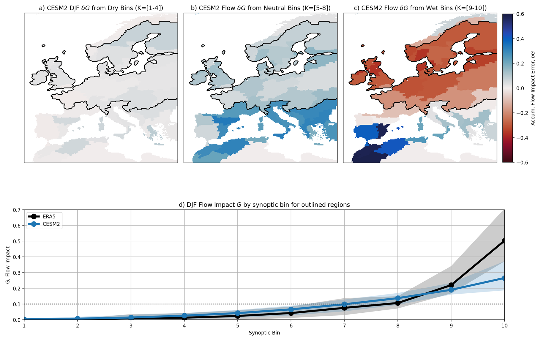
Figure 14 DJF biases in the flow impact, G_k, aggregated for the 40 % of synoptic conditions least favouring heavy precipitation (a), the middle 40 % of conditions (b) and for the 20 % of conditions that most favour heavy precipitation (c). Negative/positive biases indicate a given synoptic condition is less/more likely to cause heavy precipitation in a model than in observations, after accounting for the model's bulk bias in heavy precipitation occurrence. The black contour outlines 15 regions with large under-sensitivity to strong synoptic precursors. (d) G_k averaged over the 15 outlined regions for ERA5 and for CESM2, with the spread in values between regions indicated by shading.

Equation (6) shows that only model biases in F_k and G_k will distort forced changes. Biases in F_k will distort conversion changes whereas biases in G_k will distort dynamical and non-linear changes. As a concrete example: for the central UK and Ireland in JJA, heavy precipitation probability during strong precursors (k = 10) is 0.25 in ERA5 and 0.12 in CESM2, while the unconditional probability of heavy precipitation is 0.05 and 0.034, respectively. Therefore, for ERA5 G₁₀ = 0.25$/$0.05 = 5, while for CESM2 ${\stackrel{\mathrm{̃}}{G}}_{\mathrm{10}}$ = 0.12$/$0.034 = 3.5. This means that the flow impact of strong precursors in CESM2 is too small (${\stackrel{\mathrm{̃}}{G}}_{\mathrm{10}}-G_{\mathrm{10}}<\mathrm{0}$) and so dynamical changes in heavy precipitation due to changes in the occurrence of strong precursors, $\mathrm{\Delta }{P}_{S_{\mathrm{10}}}$, will be underestimated.

For the two models considered here, the relative amplitude of errors in F and G is mostly < 20 % (that is; a ±0.01 change in heavy precipitation probability) and so provide only a minor refinement to the bulk change, as shown in Figs. S9–S11. The standout exception is for CESM2 DJF in northern Europe, where the flow-dependent decomposition reveals that changes are underestimated by as much as 50 % due to errors in the flow impact, G. Figure 14a–c shows δG = ${\sum }_k\left[{\stackrel{\mathrm{̃}}{G}}_k-G_k\right]$ summed over the lowest 4 synoptic bins (a), the middle 4 bins (b) and the top 2 bins (c). In northern Europe, CESM2 systematically underestimates the flow impact of the strongest precursors, which capture strong eastward jet anomalies, while mildly overestimating the impact of weak-to-moderate jet anomalies. Figure 14d shows the spread of G_k over these regions and highlights a systematically low sensitivity in the heavy precipitation response: changes in synoptic conditions have too little impact on heavy precipitation probability. This lack of sensitivity means that CESM2's projected increase in strong, eastward jet days in a warmer climate (cf. Fig. 12a) does not increase the model's precipitation as much as that same dynamical change would in the real world. As we live in the real world, it is the corrected precipitation change we are interested in.

Autumn forced changes in the northern Adriatic

If a model is very severely biased in a particular region we may not trust even a corrected estimate of the model's future forced changes as discussed above. However, flow decomposition can allow usable information to be extracted even in such cases. Considering again the northern Adriatic in SON, where both models showed severe conversion biases (cf. Sect. 4.2) we find that both models project future increases in heavy precipitation probability (positive net change in Fig. 15c). We can use the additive reformulation of α_k introduced in Sect. 5 to compute conversion changes of ≈ +2 %, but it is debatable whether this information should be used: the magnitude of the conversion biases indicates that the underlying real-world processes that will drive future conversion changes are simply not accounted for. The dynamical changes however can be considered quite independently. CESM2 projects negligible changes in the wave-driven dynamics that drive North Adriatic precipitation (Fig. 15a). MPI-GE shows signs of fewer mid-Mediterranean troughs and more ridges, resulting in a negative (−1 %) dynamical contribution to changes in heavy precipitation, and a negative dynamical change in every ensemble member (Fig. 15c). These dynamical changes are based on the model's dynamics and real-world precipitation conversion, and so can be considered a valid projection despite the model's conversion errors. Decomposing the overall change into these contributions allows each to be assessed and acted upon on its own merits, increasing the usability of the simulations overall.

Figure 15 As for Fig. 10 but for the northern Adriatic region in SON.

7 Discussion

Our investigation of European heavy precipitation in CESM2 and MPI-GE yields several lessons that carry broader implications.

Model biases cannot be simply subtracted or divided out

As we have shown in Sects. 5 and 6, flow-dependent biases – especially compensating biases – can distort changes. In the worst case, these distortions can be of the same magnitude as the true change. This was the case for CESM2's projections of wintertime heavy precipitation: the model's projected strengthening of the wintertime jet would imply an increase in northern European heavy precipitation probability 30 %–60 % larger than direct model output indicates, given the observed synoptic-to-precipitation relationship.

Compensating biases are widespread

Errors in a model's synoptic circulation often partially cancel out deficiencies in the conversion of dynamical forcing into heavy precipitation by mesoscale, boundary layer, land surface, thermodynamic and/or microphysical processes (cf. Fig. 9). In these cases, models are less trustworthy than they initially appear, and improvements of model processes may worsen their bulk performance. This could explain the unexpectedly poor results from increasing model resolution without retuning, and warns that expensive regional downscaling efforts may prove disappointing when driven by models with compensating errors. While regional modellers select global models with an eye to dynamical biases (Sobolowski et al., 2025), this focus is mostly limited to mean biases and dominant variability modes, which can hide compensating errors. With a flow-dependent decomposition of precipitation, we can identify, explain and quantify these and other cases, visualising them either in a 2D space (e.g. Fig. 5d) or on a map (e.g. Fig. 9).

Flow-dependent model biases can be categorised to inform the downscaling and climate services communities

While the exact thresholds used to define categories should be tuned to different use cases, the practical interpretation of these conceptual categories remains the same:

1. Minimal bias. With both realistic dynamics and conversion processes, regional precipitation from the model can be used at face-value.

2. Conversion bias. Deficiencies in conversion processes but accurate large-scale dynamics make this model an excellent candidate for regional downscaling.

3. Dynamical bias. Accurate conversion of dynamical forcing into precipitation but a skewed distribution of synoptic circulations mean the model could be useful for storyline analysis, but should not be used to derive bulk probabilities or drive regional simulations unless nudging or bias correction techniques are employed.

4. Compounding bias. The physical realism of this model for the region is better than it appears, and could be somewhat improved by downscaling or improving model processes.

5. compensating bias. The model should be used with caution in this region and can be expected to actively worsen locally when improvements are made to either the large-scale circulation or the conversion processes alone.

Apparent agreement on bulk statistics between models can be misleading

As demonstrated (cf. Fig. 10), models may produce the same net change while representing very different futures, with different narratives for how weather and climate evolve. Different future scenarios can be efficiently distinguished with flow-dependent metrics and quickly visualised with a categorisation of forced changes, just as for biases:

1. Minimal change. Future heavy precipitation will resemble the present.

2. Conversion change. Individual synoptic conditions can be expected to become more/less reliably extreme, altering precipitation volatility.

3. Dynamical change. Heavy precipitation will be caused by a change in the frequency of synoptic conditions, each behaving the same as today.

4. Compounding change. Heavy precipitation will increase due to a greater number of more extreme synoptic conditions, or decrease due to fewer, less extreme conditions.

5. Compensating change. Fewer, stronger synoptic conditions or (rarely) more frequent but weaker conditions. The former case poses the greater risk for historically unseen precipitation extremes.

Flow-dependent approaches can make biased models more useful

Decomposing model behaviour is not simply a way to critique existing climate simulations, but offers opportunities to improve their value. For moderate biases, we have shown how flow-dependent decomposition provides a flow-aware bias correction and recalibration of forced changes. Even when models arguably cannot represent regional conversion processes well enough to simulate their future change, as we suggest for the North Adriatic region (cf. Figs. 6 and 15), the dynamical component of heavy precipitation change can still be isolated and understood.

8 Conclusions and outlook

How can we understand the enormous complexity and spatiotemporal heterogeneity of precipitation in climate models? This study has tackled this question with an eye to both informing model development and ensuring existing projections can be well used, focusing on biases and changes in European daily heavy precipitation in large-ensemble experiments from two leading climate models.

We introduced a multi-scale, flow-dependent decomposition, analysing separately biases and forced changes in the synoptic dynamics that cause precipitation and in the of conversion of those dynamics into heavy precipitation. Dynamics are represented by flow-precursors that efficiently encode the most important local precipitation-causing processes, enabling us to provide a comprehensive 4-season analysis covering 38 regions. Our precursor-based decomposition identifies a more central role for synoptic dynamics in explaining biases and changes in heavy precipitation than previous decomposition methods based on regimes or flow analogues, although differences in the decomposition formula, event definition and specific climate models used may also play a role.

We show that compensating biases and changes between scales are common, that these have serious implications for model assessment and interpretation, and that our flow-dependent approach is well suited to understanding these. We also demonstrate that apparent agreement on future precipitation changes between models can arise from very different sources, indicating a lack of a coherent, trustworthy storyline of future change which may not be evident when aggregating changes across different weather patterns and scales. We propose a categorisation of model biases and changes that supports quick identification of such “hidden” biases and model disagreements. To make the details of this analysis as accessible and interpretable as possible, we have developed an interactive interface to visualise our results: https://uib-precursors-cmip6-interactive.hf.space/app (last access: 17 April 2026).

A natural next step is to extend this two-model analysis to the full range of CMIP6 and soon-to-come CMIP7 simulations, providing a breakdown of structural uncertainties in precipitation projections that can support the next IPCC assessment. Our results showed high variability in future changes across ensemble members, emphasising the importance of ensemble projections. For single member or small-ensemble simulations, limiting the flow decomposition to a smaller number of synoptic bins (e.g. k = 5) can decrease sampling error by ≈ 20 % but at the cost of decreasing the accuracy of the decomposition. Indeed, for large ensembles a larger number of synoptic bins may be justifiable, as supplementary analysis has revealed small but systematic refinements in the decomposition when using k = 20, for JJA in particular.

The general framework of our approach could be easily extended beyond Europe to other mid-latitude regions, to other precipitation metrics, and beyond precipitation to any surface hazard strongly conditioned on synoptic dynamics, such as wind gusts or wildfires. While we consider only the occurrence of heavy rainfall rather than rainfall intensity, the two quantities are closely related in models. Our results therefore also expose where the quantity of heavy precipitation may change. In subtropical regions, and to some extent the midlatitude summer, heavy precipitation is less organised by synoptic dynamics and has stronger upscale feedbacks. In these contexts the use of time-lagged precursors as in Dorrington et al. (2024a) may prove important to clearly establish causality. Extending the precursor approach down to the hourly timescale and to include 3-dimensional mesoscale dynamics is another area that could yield insights, given the episodic nature of heavy precipitation.

A final exciting prospect is to apply our analysis to the increasing volume of convection permitting regional simulations over Europe, which inherit much of their large scale dynamics from the driving global climate models, but promise to resolve the local conversion processes more faithfully. The forced change budget we derived can combine information from a variety of sources, allowing one to compute dynamical precipitation changes from large ensemble output and conversion changes from convection-permitting regional models, for example. Such a quantitative synthesis of the increasingly diverse climate modelling landscape is currently lacking.

Appendix A: Extended derivation of precipitation decomposition

In this appendix we expand upon and consolidate the derivation of the bias and change decomposition introduced in the main text, and discuss a small number of special cases which ultimately had a negligible role in our analysis of CESM2 and MPI-GE, but may have more relevance in other contexts.

A1 Decomposition

We represent the observed probability of a particular hazard H, as conditional on some parameterisation of the large-scale flow S:

$$\begin{array}{}\text{(A1)}& P_H=\underset{-\mathrm{\infty }}{\overset{\mathrm{\infty }}{\int }}P\left(H\right|S)\cdot P(S)\mathrm{d}s.\end{array}$$

To allow empirical estimation of both P(H|S) and P(S) we discretise into N bins, indexed k, where the equality with P_H is still exact but where the decomposition into P_S and P_H|S is now approximate:

$$\begin{array}{c}{\displaystyle }{P}_H=\sum _k{P}_{H|S_k}\cdot P_{S_k}\\ {\displaystyle }\mathrm{1}=\sum _k{P}_{S_k}\end{array}$$

This formulation is now mathematically equivalent to e.g. a decomposition into N categorical flow regimes, although of course the exact choice of S will significantly impact the results. We define S by discretising the first principal component of Z500, U850 and V850 precursor indices into N evenly spaced quantiles. This decomposition is then specific to a given season and region.

Throughout we will denote biased model quantities using tildes, and future quantities (whether model or best real-world estimate) with asterisks. We denote $P_{S_k}$ as the dynamical term and $P_{H|S_k}$ as the conversion term. For an imperfect model with hazard probability ${\stackrel{\mathrm{̃}}{P}}_H$ we represent errors in the occurrence frequency of the synoptic states {S_k} as additive errors $\mathit{\delta }{P}_{S_k}$. We represent errors in the conditional conversion term as multiplicative errors ξ_k, which is a choice informed by the known dynamics of precipitation. As such:

$$\begin{array}{}\text{(A2)}& {\stackrel{\mathrm{̃}}{P}}_H=\sum _k\left(P_{H|S_k}\left[\mathrm{1}+{\mathit{\xi }}_k\right]\right)\cdot \left(P_{S_k}+\mathit{\delta }{P}_{S_k}\right).\end{array}$$

To consider forced changes, we denote the future hazard probability of the model as $P_H^{*}$, and again formulate dynamical changes, $\mathrm{\Delta }{P}_{S_k}$, as additive and conversion changes, α_k, as multiplicative. Rewriting $P_H^{*}$ in terms of deviations from the observed P_H caused by both biases and forced changes we obtain:

$$\begin{array}{}\text{(A3)}& {\stackrel{\mathrm{̃}}{P}}_H^{*}=\sum _k\left(P_{H|S_k}\left[\mathrm{1}+{\mathit{\xi }}_k\right]\left[\mathrm{1}+{\mathit{\alpha }}_k\right]\right)\cdot \left(P_{S_k}+\mathit{\delta }{P}_{S_k}+\mathrm{\Delta }{P}_{S_k}\right).\end{array}$$

Why replace the concise left hand side of this equation with a lengthy decomposition? Ultimately, we wish to know the future real-world hazard probability $P_H^{*}$, but this is inaccessible to us—we only have estimates from imperfect models. While there are surely errors in the model changes $\mathrm{\Delta }{P}_{S_k}$ and α_k, we have no way to identify these a priori. Ultimately we must trust some aspect of the model output or else we cannot proceed. Our contention is that errors in the decomposed, synoptically-conditioned changes {α_k} and {ΔP_k} will be smaller, in aggregate, than the change error coming from a direct bulk computation ${\stackrel{\mathrm{̃}}{P}}_H^{*}/{\stackrel{\mathrm{̃}}{P}}_H$. As the bulk change is simply the aggregate of changes under different conditions, then errors in the bulk change error can only be smaller if the flow-dependent errors cancel each other out. This would be a shaky scenario to rely upon. In Sect. A2 we consider the possibility of time-varying biases model bias. However if we accept the above hypothesis that flow dependent changes provide a more trustworthy assessment of future change, and consider the flow-dependent model biases to be stationary, it is useful to rewrite Eq. (A3) as:

$$\begin{array}{}\text{(A4)}& \begin{array}{rl}{\stackrel{\mathrm{̃}}{P}}_H^{\ast }=& \sum _k[\\ & \underset{\text{Observed reference}}{\underbrace{P_{H|S_k}\cdot P_{S_k}}}\\ +& \underset{\text{Historical model bias}}{\underbrace{P_{H|S_k}\left[\mathit{\delta }{P}_{S_k}+{\mathit{\xi }}_k\left(P_{S_k}+\mathit{\delta }{P}_{s_k}\right)\right]}}+\\ +& \underset{\text{Adjusted model change}}{\underbrace{P_{H|S_k}\left[{\mathit{\alpha }}_k{P}_{S_k}+\mathrm{\Delta }{P}_{S_k}\left(\mathrm{1}+{\mathit{\alpha }}_k\right)\right]}}\\ +& \mathrm{\Delta }{P}_{H_k,\mathrm{\text{spurious}}}]\end{array}\end{array}$$

Where the last term is the spurious model change:

$$\begin{array}{}\text{(A5)}& \begin{array}{rl}\mathrm{\Delta }{P}_{H_k,\mathrm{\text{spurious}}}=& P_{H|S_k}[\\ +& \underset{\text{Dynamical error}}{\underbrace{{\mathit{\alpha }}_k\cdot \mathit{\delta }{P}_{S_k}}}\\ +& \underset{\text{Thermodynamic error}}{\underbrace{{\mathit{\xi }}_k\left[{\mathit{\alpha }}_k\cdot P_{S_k}+(\mathrm{1}+{\mathit{\alpha }}_k)\cdot \mathrm{\Delta }{P}_{S_k}\right]}}\\ +& \underset{\text{non-linear error}}{\underbrace{{\mathit{\xi }}_k{\mathit{\alpha }}_k\cdot \mathit{\delta }{P}_{S_k}}}]\end{array}\end{array}$$

We see that the observed conversion rate for a given synoptic state, $P_{H|S_k}$, factors out completely from all terms, meaning that changes and biases in states where $P_{H|S_k}$ is large will have greater importance. We now have 4 groupings of terms. The first is simply the observational reference. The three terms in the second grouping contain the dynamical, conversion and non-linear contributions to model bias respectively. The third grouping contains all terms which contain a change in hazard, but with no contribution from model bias. They therefore tell us what the model implies about real-world hazard changes. Finally, the fourth grouping of terms contains products of changes and model bias. We consider these last terms to be spurious changes as they represent changes in future hazard probability that are not consistent with our current observed reality. If hazard changes are considered as additive then the differences between the bulk change, ${\stackrel{\mathrm{̃}}{P}}_H^{*}-{\stackrel{\mathrm{̃}}{P}}_H$, and the flow-dependent change is simply this fourth group of terms. However, precipitation changes are typically considered as multiplicative:

$$\begin{array}{}\text{(A6)}& \stackrel{\mathrm{̃}}{\mathit{\beta }}={\displaystyle \frac{{\stackrel{\mathrm{̃}}{P}}_H^{*}}{{\stackrel{\mathrm{̃}}{P}}_H}}-\mathrm{1},\end{array}$$

where $\stackrel{\mathrm{̃}}{\mathit{\beta }}$ is the bulk multiplicative change. The flow-dependent multiplicative change is simply:

$$\begin{array}{}\text{(A7)}& \mathit{\beta }={\displaystyle \frac{{\sum }_k{P}_{H|S_k}\left[{\mathit{\alpha }}_k{P}_{S_k}+\mathrm{\Delta }{P}_{S_k}\left(\mathrm{1}+{\mathit{\alpha }}_k\right)\right]}{P_H}}\end{array}$$

but now computing $\stackrel{\mathrm{̃}}{\mathit{\beta }}-\mathit{\beta }$ is complicated by the different denominators in Eqs. (A6) and (A7), which mean the spurious terms cannot be directly disentangled into conversion and dynamical contributions. However we can proceed as follows:

$$\begin{array}{}\text{(A8)}& {\displaystyle }\begin{array}{rl}\stackrel{\mathrm{̃}}{\mathit{\beta }}-\mathit{\beta }=& {\displaystyle \frac{{\sum }_k{\stackrel{\mathrm{̃}}{P}}_{H|S_k}\cdot \left({\stackrel{\mathrm{̃}}{P}}_{S_k}+\mathrm{\Delta }{P}_{S_k}\right)\cdot \left(\mathrm{1}+{\mathit{\alpha }}_k\right)}{{\stackrel{\mathrm{̃}}{P}}_H}}\\ & -{\displaystyle \frac{{\sum }_k{P}_{H|S_k}\cdot \left(P_{S_k}+\mathrm{\Delta }{P}_{S_k}\right)\cdot \left(\mathrm{1}+{\mathit{\alpha }}_k\right)}{P_H}}\end{array}\text{(A9)}& {\displaystyle }\begin{array}{rl}=& \sum _k\left[\mathrm{\Delta }{P}_{S_k}\cdot \left(\mathrm{1}+{\mathit{\alpha }}_k\right)\left[{\displaystyle \frac{{\stackrel{\mathrm{̃}}{P}}_{H|S_k}}{{\stackrel{\mathrm{̃}}{P}}_H}}-{\displaystyle \frac{P_{H|S_k}}{P_H}}\right]\right.\\ & \left.+{\mathit{\alpha }}_k\left[{\displaystyle \frac{{\stackrel{\mathrm{̃}}{P}}_{H|S_k}\cdot {\stackrel{\mathrm{̃}}{P}}_{S_k}}{{\stackrel{\mathrm{̃}}{P}}_H}}-{\displaystyle \frac{P_{H|S_k}\cdot P_{S_k}}{P_H}}\right]\right]\end{array}\text{(A10)}& {\displaystyle }\equiv \sum _k\left[\mathrm{\Delta }{P}_{S_k}\cdot \left(\mathrm{1}+{\mathit{\alpha }}_k\right)\left[{\stackrel{\mathrm{̃}}{G}}_k-G_k\right]+{\mathit{\alpha }}_k\left[{\stackrel{\mathrm{̃}}{F}}_k-F_k\right]\right]\end{array}$$

Where in Eq. (17) we have newly defined F_k and G_k, which we term the flow relevance and flow impact respectively. Both new terms can be written in alternate forms, which aids with their interpretation:

$$F_k={\displaystyle \frac{P_{H|S_k}\cdot P_{S_k}}{P_H}}=P_{S_k|H}{G}_k={\displaystyle \frac{P_{H|S_k}}{P_H}}={\displaystyle \frac{P_{S_k|H}}{P_{S_k}}}$$

The same alternate forms hold for ${\stackrel{\mathrm{̃}}{F}}_k$ and ${\stackrel{\mathrm{̃}}{G}}_k$, with tildes on all quantities. The flow relevance is therefore the fraction of hazard events that occur within a particular synoptic bin, while the flow impact is the conditional odds ratio of a hazard.

Additive errors in G_k and F_k weighted by the flow-dependent forced changes explain the differences between the net bulk and flow dependent multiplicative changes. If a model has constant conversion bias (that is ξ_k = ξ ∀ k) then ${\stackrel{\mathrm{̃}}{G}}_k=G_k$ and dynamical changes are not distorted. However even under these conditions, nonzero dynamical bias will still result in distortions in conversion changes.

A2 Time evolving biases

Equation (A3) is based on the assumption that model biases in the occurrence of synoptic weather patterns, $\mathit{\delta }{P}_{S_k}$, and in the occurrence of heavy precipitation under a weather pattern, ξ_k, are stationary in time. Section 5 discusses how bias-change cross terms can be thought of as time-evolving biases due to changing occurrences of synoptic states. However as pointed out in e.g. Maraun (2012), a new climate state might result in models being biased in new ways if, for example, there is a forced change in the ratio of cloud types a model has biases in those cloud processes. To address this, we can extend Eq. (A3) to include a further set of changes in conversion and dynamics, Δξ_k and $\mathrm{\Delta }\mathit{\delta }{P}_{S_k}$ respectively:

$$\begin{array}{}\text{(A11)}& \begin{array}{rl}{\stackrel{\mathrm{̃}}{P}}_H^{*}& =\sum _k\left(P_{H|S_k}\left[\mathrm{1}+{\mathit{\xi }}_k\right]\left[\mathrm{1}+\mathrm{\Delta }{\mathit{\xi }}_k\right]\left[\mathrm{1}+{\mathit{\alpha }}_k\right]\right)\\ & \cdot \left(P_{S_k}+\mathit{\delta }{P}_{S_k}+\mathrm{\Delta }\mathit{\delta }{P}_{S_k}+\mathrm{\Delta }{P}_{S_k}\right)\end{array}\end{array}$$

These new terms can be interpreted in two ways: we could consider $\mathit{\delta }{P}_{S_k}+\mathrm{\Delta }\mathit{\delta }{P}_{S_k}$ as representing a time evolving bias superimposed on the true climate response $\mathrm{\Delta }{P}_{S_k}$, or we could consider a modelled climate response $\mathrm{\Delta }{P}_{S_k}+\mathrm{\Delta }\mathit{\delta }{P}_{S_k}$ with true and spurious components, superimposed on a stationary bias $\mathit{\delta }{P}_{S_k}$. The same consideration can be given to the conversion terms. As such, non-stationary bias and spurious climate trends are mathematically equivalent and can be viewed as interchangeable ideas in the absence of any concrete physical hypothesis for a particular model and region/season.

If we view Δξ_k and $\mathrm{\Delta }\mathit{\delta }{P}_{S_k}$ as spurious changes, but acknowledge that in general we have no way to disentangle them from the true forced changes, α_k and $\mathrm{\Delta }{P}_{S_k}$, then we can set them to 0, and return to Eq. (A3). However, if through prior analysis we have obtained some emergent constraint or isolated a known process-dependent bias then this can be used to specify any or all of the terms Δξ_k and $\mathrm{\Delta }\mathit{\delta }{P}_{S_k}$ as a known quantity. These known non-stationary biases/spurious trends can then be grouped with the historical bias terms, and Eq. (A4) can be applied as written.

A3 Novel synoptic conditions

In principle it is possible for a model to produce a novel synoptic state entirely outside the observed distribution, which we can assign to a new bin n. The frequency of occurrence of these conditions is δP_S,n and where for lack of more information we assume ξ_n=0:

$$\begin{array}{}\text{(A12)}& {\stackrel{\mathrm{̃}}{P}}_{H,n}^{*}={\stackrel{\mathrm{̃}}{P}}_{H|S_n}\mathit{\delta }{P}_{S_n}+{\stackrel{\mathrm{̃}}{P}}_{H|S_n}\mathrm{\Delta }{P}_{S_n}\left[\mathrm{1}+{\mathit{\alpha }}_n\right]+{\mathit{\alpha }}_n{\stackrel{\mathrm{̃}}{P}}_{H|S_n}\mathit{\delta }{P}_{S_n}\end{array}$$

which gives us the bias, the adjusted trend, and the spurious trend respectively. If novel synoptic states occur in the future simulations only, then we can estimate none of the biases or the trends, and so we can only include the contribution of the bin as a whole: $P_H^{*}$ = ${\sum }_k{P}_{H_k}^{*}$ = $P_{H_n}^{*}$. In fact, novel states have no impact in the two models we consider in this paper, and so they are not included in our main analysis. However we cannot rule out their relevance for more severely biased models or in more extreme climate scenarios.

A4 Conversion changes under severe bias

α_k is formulated as multiplicative, but this can cause issues if $P_{H|S_k},P_{H|S_k}^{*}\gg {\stackrel{\mathrm{̃}}{P}}_{H|S_k}$, that is, if the historical simulation shows near-zero conversion for a particular weather pattern but does exhibit conversion in a future climate. As a concrete example, consider $P_{H|S_k}=\mathrm{0.04}$, ${\stackrel{\mathrm{̃}}{P}}_{H|S_k}=\mathrm{0.002}$ and $P_{H|S_k}^{*}=\mathrm{0.02}$. A direct reading of this would give α=10 and an estimate of real-world future hazard probability rising from 4 % to 40 %. This is clearly unrealistic, and in most cases conversion changes under such conditions should be disregarded as uninformative. However for completeness and to handle border-line cases, we model conversion changes as additive when 1+ξ_k is close to zero:

$$\begin{array}{}\text{(A13)}& \begin{array}{rl}{P}_{S_k}& P_{H|S_k}^{\ast }=P_{S_k}{P}_{H|S_k}\cdot (\mathrm{1}+{\mathit{\alpha }}_k)=\\ & \left.\begin{array}{lr}{P}_{S_k}{P}_{H|S_k}\left(\frac{{\stackrel{\mathrm{̃}}{P}}_{H|S_k}^{\ast }}{{\stackrel{\mathrm{̃}}{P}}_{H|S_k}}\right),& \text{for }\mathit{\xi }\gg -\mathrm{1}\\ P_{S_k}{P}_{H|S_k}\left(\mathrm{1}+\frac{{\stackrel{\mathrm{̃}}{P}}_{H|S_k}^{\ast }-{\stackrel{\mathrm{̃}}{P}}_{H|S_k}}{P_{H|S_k}}\right),& \text{for }\mathit{\xi }\approx -\mathrm{1}\end{array}\right\}\end{array}\end{array}$$

To avoid a sharp switch in the algorithm which might be sensitive to resampling or parameter values and can distort ensemble spread, we compute α with a blending function:

$$\begin{array}{}\text{(A14)}& {\mathit{\alpha }}_k=\left(\mathrm{1}-w\left({\mathit{\xi }}_k\right)\right)\cdot {\displaystyle \frac{{\stackrel{\mathrm{̃}}{P}}_{H|S_k}^{*}}{P_{H|S_k}}}+w\left({\mathit{\xi }}_k\right)\cdot \left({\displaystyle \frac{{\stackrel{\mathrm{̃}}{P}}_{H|S_k}^{*}}{{\stackrel{\mathrm{̃}}{P}}_{H|S_k}}}-\mathrm{1}\right),\end{array}$$

where

$$\begin{array}{}\text{(A15)}& w\left(\mathit{\xi }\right)={\displaystyle \frac{(\mathrm{1}+\mathit{\xi }{)}^{\mathrm{4}}}{(\mathrm{1}+\mathit{\xi }{)}^{\mathrm{4}}+{\mathrm{0.1}}^{\mathrm{4}}}}.\end{array}$$

For small or positive conversion biases w = 1 with a deviation of only ${\left(\frac{\mathrm{0.1}}{\mathrm{1}+\mathit{\xi }}\right)}^{\mathrm{4}}$, while for strong negative bias, w = 0 with an deviation of only ${\left(\frac{\mathrm{1}+\mathit{\xi }}{\mathrm{0.1}}\right)}^{\mathrm{4}}$. Testing has showed this reduces sensitivity of the decomposition results to the number of bins chosen and gives more “sensible” results for these special cases.