Persistent SST anomaly vs. dynamical ocean model in winter weather forecasts: Global Ensemble Prediction System versions 5 and 6 over the North Pacific and North Atlantic

The impact of coupling an atmosphere model to a dynamical ocean model, rather than using persistent SST anomalies, is assessed for wintertime medium-range forecasts over the North Pacific and North Atlantic. This assessment is based on 20 years (1998–2017) of hindcasts produced by the Global Ensemble Prediction System (GEPS) of Environment and Climate Change Canada (ECCC). We compare an uncoupled atmospheric model (versions 5, GEPS5) with an atmosphere–ocean coupled model (version 6, GEPS6) alongside European Centre for Medium-Range Weather Forecasts Reanalysis v5 (ERA5) as the verification dataset. We find that by the third pentad, or days 11–15, coupling to a dynamic ocean model weakens the Aleutian Low, the Icelandic Low, and the Atlantic Subtropical High. This produces less integrated vapor transport (IVT) over the Pacific and Atlantic Oceans, whose spatial patterns are modulated by phases of Madden–Julian Oscillation (MJO). Coupling also results in colder sea surface temperature (SST) over the Kuroshio Current Extension region and produces a weaker Aleutian Low due to less upward latent heat fluxes. The weaker Aleutian Low further reinforces its weakening through a positive feedback loop. Lastly, the coupling to a dynamical ocean reduces the latent heat flux bias variance by 10 %–20 %, thus improving the IVT.

1 Introduction

Improving medium-range forecasts (5–15 d) remains critical to better prepare society for weather extremes. The time-evolving ocean state is a crucial element needed to correctly simulate strong weather variability, such as the Madden–Julian Oscillation (MJO; Madden and Julian, 1971; Wheeler and Hendon, 2004) and atmospheric rivers (ARs; Gimeno et al., 2014), that are important signals in subseasonal-to-seasonal (S2S) precipitation forecasts (Subramanian et al., 2019). Mid-latitude cyclones can cause strong sea surface temperature (SST) perturbations (Hsu et al., 2024) approximately 10 d after passage (Kobashi et al., 2019) and feed back to the storm tracks (Booth et al., 2012). Major weather agencies have adopted high-resolution (less than 50 km) coupled systems for medium-range forecasts and have shown detectable improvement in forecast skill through their use (Brassington et al., 2015). The benefit often comes from the tropics, where cloud convection is an important source of available potential energy and is sensitive to SST.

Since air–sea fluxes are modulated by near-surface wind speed, two-way air–sea coupling measurably improves tropical cyclone forecasts. The SST cooling induced by wind-driven ocean mixed-layer deepening and Ekman upwelling can feed back in a few days to reduce storm intensity (Rainaud et al., 2017; Smith et al., 2018; Sun et al., 2023; Polichtchouk et al., 2025). Similarly, coupling is also known to have a positive impact on MJO prediction (DeMott et al., 2015; Savarin and Chen, 2022) because SST cooling due to wind anomalies and the diurnal variation of mixed-layer depth can modulate MJO propagation speed and intensity. The ability to predict the MJO is particularly important because it is known to remotely modulate the North Atlantic Oscillation (NAO) (Cassou, 2008; Lin et al., 2009; Scaife et al., 2017) and to influence global temperature and precipitation on a subseasonal timescale (Stan et al., 2017).

Coupled models have advanced to use grid sizes of less than a degree, leading to new understanding of air–sea coupling. In particular, there is a growing awareness of the role of ocean-eddy-scale air–sea interactions in high-resolution simulations where the SST gradients can effectively modify near-surface atmospheric curl, divergence, and therefore heat fluxes (Small et al., 2008; Roberts et al., 2016; Bishop et al., 2017; Liu et al., 2021; Seo et al., 2023; Renault et al., 2024). However, over western boundary current extensions coupled models do not necessarily predict the SST within eddies better than persistence (Vellinga et al., 2020), contributing to systematic errors in medium-range forecasts.

The hindcasts of the Global Ensemble Prediction System (GEPS) versions 5 (GEPS5) and 6 (GEPS6) of the Environment Climate Change Canada (ECCC) provided as part of the subseasonal-to-seasonal (S2S) project (Vitart et al., 2017) are useful data for assessing atmospheric response to the ocean. Because GEPS5 uses persistent SST anomaly and GEPS6 couples with Nucleus for European Modelling of the Ocean (NEMO; Madec, 2008), contrasts between them reveal the impact of using a dynamical ocean model in place of prescribed SST. Previous documentation (Lin et al., 2019) (see Supplement for the hyperlink) compared 20-year hindcasts of these two models and found improvements of GEPS6 in multiple metrics during winter, including better Arctic sea ice in the Pacific and Eurasian sectors, surface air temperature, tropical SST, and MJO activity. However, there has been less evaluation of the North Pacific and North Atlantic, where the Kuroshio Current Extension and Gulf Stream strongly influence air–sea exchange and weather activities.

In this study, we assess the impact of replacing persistent SST anomalies with a dynamical ocean model in the North Pacific and North Atlantic during the winter using 20 years of hindcast data. We use integrated vapor transport (IVT; Rutz et al., 2014) as a proxy to assess weather extremes due to its connection with atmospheric rivers (ARs; Zhu and Newell, 1994; Gimeno et al., 2014; Rutz et al., 2014; Guan and Waliser, 2015; Pasquier et al., 2019; Waliser and Guan, 2017). Overall, we have three main findings. First, the use of a dynamical ocean in GEPS6 weakens the Aleutian Low, the Icelandic Low, and the Atlantic Subtropical High, subsequently resulting in a weaker IVT, with a spatial pattern influenced by the MJO. Second, the colder initial SST in GEPS6 over the Kuroshio Current Extension generates a weaker Aleutian Low, which further weakens itself through a positive feedback loop. Third, the air–sea coupling reduces the latent heat flux bias variance by 10 %–20 % and improves the IVT forecast over the Kuroshio Current Extension, especially during MJO phases 5–8.

In Sect. 2, we introduce our datasets and methodology. Section 3 presents and discusses our results. In Sect. 4, we draw conclusions.

2 Dataset and Methods

2.1 Global Ensemble Prediction System (GEPS)

GEPS5 uses the Global Environmental Multiscale (GEM) atmospheric model (Côté et al., 1998a, b). GEPS5 has 45 vertical levels using log-pressure vertical coordinate (Girard et al., 2014), and uses the Ying–Yang grid with a horizontal resolution of 39 km (Qaddouri and Lee, 2011). For the ocean boundary condition, GEPS5 uses the persistent anomaly method: on top of the climatological seasonal cycle, the 30 d average SST anomaly preceding the initial date derived from ERA-Interim is added and persists throughout the integration (Lin et al., 2016). The sea ice cover is adjusted according to local SST so that the resulting sea ice cover and SST are consistent (Gagnon et al., 2014). The initial conditions are obtained using an Ensemble Kalman-filter (EnKF; Houtekamer et al., 2009, 2014), with a digital filter (Fillion et al., 1995) and incremental analysis updates (Bloom et al., 1996) to reduce the shock during data assimilation (Deng et al., 2018).

GEPS6 is built on top of GEPS5 by replacing the simple statistical SST and sea ice model with a dynamical ocean and sea ice model. The ocean model is NEMO version 3.6 (Madec, 2008). NEMO uses z-level vertical coordinates, with hydrostatic, Boussinesq approximations and a linear free surface. This version has a horizontal resolution of 0.25° ORCA grid (Bernard et al., 2006, a global tripolar grid configured to remove singularity of poles of a sphere) and 50 levels increasing from 1 m at the surface to 500 m at the deepest level. The sea ice model is the Los Alamos multi-category Community Ice Model version 4 (CICE4; Hunke, 2001; Lipscomb et al., 2007; Hunke et al., 2015). The initial conditions are obtained using the EnKF, with European Centre for Medium-Range Weather Forecasts hybrid (ECMWF-hybrid) gain applied to recenter ensemble members around the means of EnKF analysis and 4DEnVar analysis (Penny, 2014; Houtekamer et al., 2019). The 4DEnVar is a 4-dimensional variational data assimilation using the Global Deterministic Prediction System (Buehner et al., 2015; Lin et al., 2019). The SST is initialized with a monthly average Ocean Reanalysis Pilot 5 (ORAP5; Zuo et al., 2017) product. The initial sea ice conditions are obtained from HadISST (Rayner et al., 2003).

For more detailed documentation, see Peterson et al. (2022) and Smith et al. (2018). Ensemble methods are described by Deng et al. (2018) for GEPS5 and Lin et al. (2019) for GEPS6.

2.2 Hindcast Data

The S2S project provides up to 60 lead days hindcasts (Vitart et al., 2008, 2017) from 13 different meteorological agencies. ECCC has contributed hindcast data from GEPS5 and GEPS6 from 1998–2017.

The hindcasts are produced operationally on a weekly basis for GEPS5 and GEPS6. For each hindcast date, hindcasts corresponding to the same date were generated for 20 years 1998–2017. Each hindcast has a lead time of 32 d with 4 ensemble members. For GEPS6, the hindcast is generated such that it has twice as many start dates as the GEPS5 hindcast, as documented in Tables S1 and S2 in the Supplement. We subsample the GEPS6 hindcast by choosing the closest start date (underlined in Table S2) to GEPS5. In our focus months, December, January, and February, the resulting start times of GEPS6 are exactly one day earlier than those of GEPS5, and start dates are spaced by 7 d. This strategy minimizes the impact of the start time difference and ensures that the GEPS6 subset has the same amount of data as GEPS5.

As our verification dataset, we use European Centre for Medium-Range Weather Forecasts (ECMWF) Reanalysis v5 (ERA5; Hersbach et al., 2020). In the Pacific and Atlantic Oceans, it can well capture offshore diurnal SST cycles under various wind conditions (Yao et al., 2021). Over Europe, the wind variability is skillfully predicted (Molina et al., 2021; Chen et al., 2024). Over North America, Chen et al. (2024) shows that ERA5 has skills in producing wind and precipitation associated with extra-tropical cyclones, with a tendency to underestimate high winds and overestimate low winds. A study over the Red Sea shows ERA5 is challenged by land–sea induced local dynamics (Alkhalidi et al., 2025).

2.3 Error Assessment Methods

Ideally, the impact of using a dynamical ocean model can be revealed by taking the difference between hindcasts of GEPS5 and GEPS6. However, the start dates of these two sets of output differ by exactly 1 d in our time of interests. Therefore, we reference both fields to ERA5 by computing the difference between GEPS and ERA5 data and then sorting the runs by start month. Differences in transient weather systems between the two initializations are not negligible, making the raw differences between GEPS6 and GEPS5 hard to interpret. By taking the difference with ERA5, we effectively remove much of the variance added from the differing transients, thus allowing for a better comparison. We have documented details in the Supplement (Sect. S2).

We first define the pentad bias

$$\begin{array}{}\text{(1)}& \begin{array}{rl}& {\mathit{\beta }}_{\mathrm{pdt},X}\left(\mathit{r},t_{\mathrm{s}},p,\mathit{\gamma }\right)=\\ & {\left(\mathrm{\Delta }w\right)}^{-\mathrm{1}}\underset{t_{\mathrm{l}}=\left(p-\mathrm{1}\right)\mathrm{\Delta }w}{\overset{p\mathrm{\Delta }w}{\int }}{X}_{\mathrm{pdt},\mathrm{hcst}}\left(\mathit{r},t_{\mathrm{s}},t_{\mathrm{l}},\mathit{\gamma }\right)\\ & -X_{\mathrm{ref}}\left(\mathit{r},t_{\mathrm{s}}+t_{\mathrm{l}}\right)\mathrm{d}{t}_{\mathrm{l}},\end{array}\end{array}$$

where β_pdt,X is the bias of the hindcast product “pdt” of the variable X at location r, t_s is the start time, t_l is the lead time, p is the lead pentad (starting from 1), γ is the ensemble member of a total N_γ members, and Δw=5 d is the size of the pentad. The subscript “hcst” denotes the hindcast, “ref” denotes the reference dataset that is used to verify the hindcast, i.e., ERA5 in this paper. With the 〈⋅〉 being the spatial averaging over a region S, we can separate the bias into a spatial mean 〈β_pdt,X〉 and an anomaly ${\mathit{\beta }}_{\mathrm{pdt},X}^{\prime }={\mathit{\beta }}_{\mathrm{pdt},X}-\langle {\mathit{\beta }}_{\mathrm{pdt},X}\rangle$. The averaged bias variance can then be written as the sum of mean and patterned variances. That is,

$$\begin{array}{}\text{(2)}& \langle {\mathit{\beta }}_{\mathrm{pdt},X}^{\mathrm{2}}\rangle =\stackrel{\mathrm{mean}}{\overbrace{\langle {\mathit{\beta }}_{\mathrm{pdt},X}{\rangle }^{\mathrm{2}}}}+\stackrel{\mathrm{patterned}}{\overbrace{\langle {{\mathit{\beta }}^{\prime }}_{\mathrm{pdt},X}^{\mathrm{2}}\rangle }}.\end{array}$$

Later in the text for the sake of simplicity, we define bias variance ${\mathit{ϵ}}_{\mathrm{pdt},X}=\langle {\mathit{\beta }}_{\mathrm{pdt},X}^{\mathrm{2}}\rangle$, mean bias variance ${\stackrel{\mathrm{‾}}{\mathit{ϵ}}}_{\mathrm{pdt},X}=\langle {\mathit{\beta }}_{\mathrm{pdt},X}{\rangle }^{\mathrm{2}}$, and patterned bias variance ${\stackrel{\mathrm{̃}}{\mathit{ϵ}}}_{\mathrm{pdt},X}=\langle {{\mathit{\beta }}^{\prime }}_{\mathrm{pdt},X}^{\mathrm{2}}\rangle$, with the decomposition as ${\mathit{ϵ}}_{\mathrm{pdt},X}={\stackrel{\mathrm{‾}}{\mathit{ϵ}}}_{\mathrm{pdt},X}+{\stackrel{\mathrm{̃}}{\mathit{ϵ}}}_{\mathrm{pdt},X}$.

The bias and its variance decomposition of variable X of a product pdt grouped by start time set ϕ is

$$\begin{array}{}\text{(3a)}& {\displaystyle }{B}_{\mathrm{pdt},X}\left(\mathit{r},\mathit{\varphi },p\right)=\left\{{\mathit{\beta }}_{\mathrm{pdt},X}\left(\mathit{r},t_{\mathrm{s}},p,\mathit{\gamma }\right)|t_{\mathrm{s}}\in \mathit{\varphi },\mathit{\gamma }=\mathrm{1},\mathrm{\dots },N_{\mathit{\gamma }}\right\},\text{(3b)}& {\displaystyle }{E}_{\mathrm{pdt},X}\left(S,\mathit{\varphi },p\right)=\left\{{\mathit{ϵ}}_{\mathrm{pdt},X}\left(S,t_{\mathrm{s}},p,\mathit{\gamma }\right)|t_{\mathrm{s}}\in \mathit{\varphi },\mathit{\gamma }=\mathrm{1},\mathrm{\dots },N_{\mathit{\gamma }}\right\},\text{(3c)}& {\displaystyle }{\stackrel{\mathrm{‾}}{E}}_{\mathrm{pdt},X}\left(S,\mathit{\varphi },p\right)=\left\{{\stackrel{\mathrm{‾}}{\mathit{ϵ}}}_{\mathrm{pdt},X}\left(S,t_{\mathrm{s}},p,\mathit{\gamma }\right)|t_{\mathrm{s}}\in \mathit{\varphi },\mathit{\gamma }=\mathrm{1},\mathrm{\dots },N_{\mathit{\gamma }}\right\},\text{(3d)}& {\displaystyle }{\stackrel{\mathrm{̃}}{E}}_{\mathrm{pdt},X}\left(S,\mathit{\varphi },p\right)=\left\{{\stackrel{\mathrm{̃}}{\mathit{ϵ}}}_{\mathrm{pdt},X}\left(S,t_{\mathrm{s}},p,\mathit{\gamma }\right)|t_{\mathrm{s}}\in \mathit{\varphi },\mathit{\gamma }=\mathrm{1},\mathrm{\dots },N_{\mathit{\gamma }}\right\},\end{array}$$

To test the significance, the degrees of freedom are counted by making the following two assumptions: (a) output from different start times or different ensemble members is independent, and (b) the output within the same pentad is not independent. In both GEPS5 and GEPS6, during 1998–2017 there are 4 start times in January with 4 ensemble members. Therefore, for each pentad there are $\mathrm{20}\times \mathrm{4}\times \mathrm{4}=\mathrm{320}$ degrees of freedom.

We define the bias change

$$\begin{array}{}\text{(4)}& \begin{array}{rl}\mathrm{\Delta }{B}_X\left(\mathit{r},\mathit{\varphi },p\right)=& \mathit{\mu }\left[B_{\mathrm{GEPS}\mathrm{6},X}\left(\mathit{r},\mathit{\varphi },p\right)\right]\\ & -\mathit{\mu }\left[B_{\mathrm{GEPS}\mathrm{5},X}\left(\mathit{r},\mathit{\varphi },p\right)\right],\end{array}\end{array}$$

where μ is the averaging operator over a given set, and a significance test is performed with the above-mentioned degrees of freedom. While the ΔB_X is a measure of the change in bias, it actually tells us about large-scale property differences between GEPS5 and GEPS6 simulations.

2.4 Impact of MJO Phase

To evaluate the impact of MJO phase, we define three start time groups using the outgoing-longwave-radiation (OLR)-based MJO index (OMI; Kiladis et al., 2014), a two-dimensional vector whose values are normalized principal components. When the magnitude of OMI is less than 1, the MJO is classified as inactive. When the magnitude of OMI is larger than 1, the MJO is active, and the MJO phases 1–8 are defined according to the phase angle of OMI. The MJO phase contains spatial information of the MJO: during MJO phases 1–4, the MJO convection center resides over the Indian Ocean. During MJO phases 5–8, the center is over the Maritime continent and tropical Pacific. The MJO start time groups are defined as

$$\begin{array}{}\text{(5a)}& {\displaystyle }\begin{array}{rl}{\mathit{\varphi }}_{\mathrm{NonMJO}}=& \left\{t|t\in {\mathit{\varphi }}_{\mathrm{DJF}}\text{, and the MJO is inactive more }\right.\\ & \left.\text{than half of the time in the next 15\hspace{0.17em}d.}\right\}\end{array}\text{(5b)}& {\displaystyle }\begin{array}{rl}{\mathit{\varphi }}_{\mathrm{P}\mathrm{1234}}=& \left\{t|t\in {\mathit{\varphi }}_{\mathrm{DJF}}\text{, the MJO is in phases 1–4 more }\right.\\ & \left.\text{than half of the time in the next 15\hspace{0.17em}d.}\right\}\end{array}\text{(5c)}& {\displaystyle }\begin{array}{rl}{\mathit{\varphi }}_{\mathrm{P}\mathrm{5678}}=& \left\{t|t\in {\mathit{\varphi }}_{\mathrm{DJF}}\text{, the MJO is in phases 5–8 more }\right.\\ & \left.\text{than half of the time in the next 15\hspace{0.17em}d.}\right\}\end{array}\end{array}$$

where ϕ_DJF is the set of all start times during December–January–February. The remaining start times are ambiguous, meaning that either the MJO is neither consistently inactive nor active, or the phase of MJO cannot be classed in either P1234 or P5678. Out of 1805 d of DJF during 1998–2017, there are 455 d of NonMJO, 331 d of P1234, 321 d of P5678, and 698 d that are ambiguous. (See Fig. S1 for histogram.)

3 Results

3.1 Impacts of Coupling to a Dynamical Ocean Model on SST and Circulation

We compute the bias change ΔB, i.e., the difference between GEPS6 and GEPS5, of SST, 850 hPa geopotential height Z₈₅₀, and 500 hPa geopotential height Z₅₀₀ of pentads 1–3 and present them in Fig. 1. The black boxes in Fig. 1c define the Kuroshio Current Extension (150° E–130° W, 30–50° N) and the Gulf Stream (75–15° W, 35–55° N) regions, and the magenta boxes in Fig. 1f and i define the Aleutian Low (140° E–130° W, 40–60° N), Icelandic Low (30° W–20° E, 55–70° N), and Atlantic Subtropical High (60° W–20° E, 20–50° N) regions.

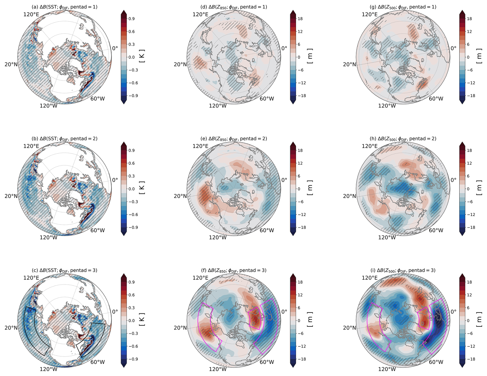
Figure 1 Bias changes ΔB of atmosphere quantities computed from Global Ensemble Forecast System (GEPS) version 5 (GEPS5) to GEPS version 6 (GEPS6) during December–January–February of the first three pentads in hindcast years 1998–2017. (a–c) ΔB of the sea surface temperature (SST) of pentad=1, 2, and 3. (d–f) Same as panels (a)–(c) but for 500 hPa geopotential height Z₈₅₀. (g–i) Same as panels (a)–(c) but for 500 hPa geopotential height Z₅₀₀. The hatched area passes the significance test of a p-value of 0.1. The black boxes in panel (c) define the Kuroshio Current Extension (150° E–130° W, 30–50° N) and Gulf Stream (75–15° W, 35–55° N) regions, and the magenta boxes in panels (f) and (i) define the Aleutian Low (140° E–130° W, 40–60° N), the Icelandic Low (30° W–20° E, 55–70° N), and the Atlantic Subtropical High (60° W–20° E, 20–50° N) regions.

The bias of the first pentad shows the impact of SST initialization (Fig. 1a) on the atmosphere (Fig. 1d and g). Over the North Pacific, the SST is colder in GEPS6, with the alternating signs around coastal Japan signifying errors in simulating the Kuroshio Current. The Z₈₅₀ shows that there is a weakening in the Aleutian Low in the middle of North Pacific, which is because of less upward latent heat flux due to a cold SST bias (Fig. 1a). In the North Atlantic, there is a similar cold bias and a northward shift of the Gulf Stream along 45° N. The impact of this shift extends northward to the edge of Arctic sea ice. The SST bias in the Gulf Stream produces a positive anomaly in Z₈₅₀ and Z₅₀₀. In the Northern Hemisphere, the difference in SST initialization strategy introduces a bias variance of about 0.05 K² (Fig. S2).

The weakening of the Aleutian Low continues in the next two pentads (Fig. 1e and f) and wanes afterward (not shown). The Atlantic basin is less straightforward. In pentad 2, the Atlantic Subtropical High starts to weaken. Meanwhile, a positive anomaly moves westward to the Atlantic (Fig. 1e and h). By pentad 3, there is a robust weakening of the Icelandic Low and the Atlantic Subtropical High (Fig. 1f and i).

The Aleutian Low weakening appears to be linked to a similar Icelandic Low weakening through a Rossby wave train (Hoskins and Karoly, 1981; Karoly, 1983). As shown in Fig. 1f and i, Z₈₅₀ and Z₅₀₀ reveal an alternating pattern of high and low centers, extending from the Aleutian Low through the Arctic to the Icelandic Low. This is consistent with Honda et al. (2001), a reanalysis study that links the influence of Aleutian Low on Icelandic Low on a subseasonal time scale, and is also widely noticed in seasonal and longer timescale (Li et al., 2024, and reference within).

The large northward shift of the Gulf Stream directly forces Z₈₅₀ and Z₅₀₀. Figure 1d and g show that there are positive geopotential anomalies at 45° N, 75° W. The anomalies persist throughout pentads 1–2.

3.2 Impacts of Coupling to a Dynamical Ocean Model on Integrated Vapor Transport (IVT)

Here, we define $\mathrm{IVT}=\left|g^{-\mathrm{1}}{\int }_{\mathrm{200}\mathrm{hPa}}^{\mathrm{1000}\mathrm{hPa}}q\mathit{v}\mathrm{d}p\right|$. Figure 2 shows the bias change ΔB of the IVT (shading) and Z₈₅₀ (contours) for pentad 3. Over the North Pacific, the IVT is reduced along the southeastern side of the weakened Aleutian Low toward the Gulf of Alaska. Over the North Atlantic, the reduced IVT lies between the weakened Icelandic Low and the Atlantic Subtropical High, with a more zonal orientation toward western Europe.

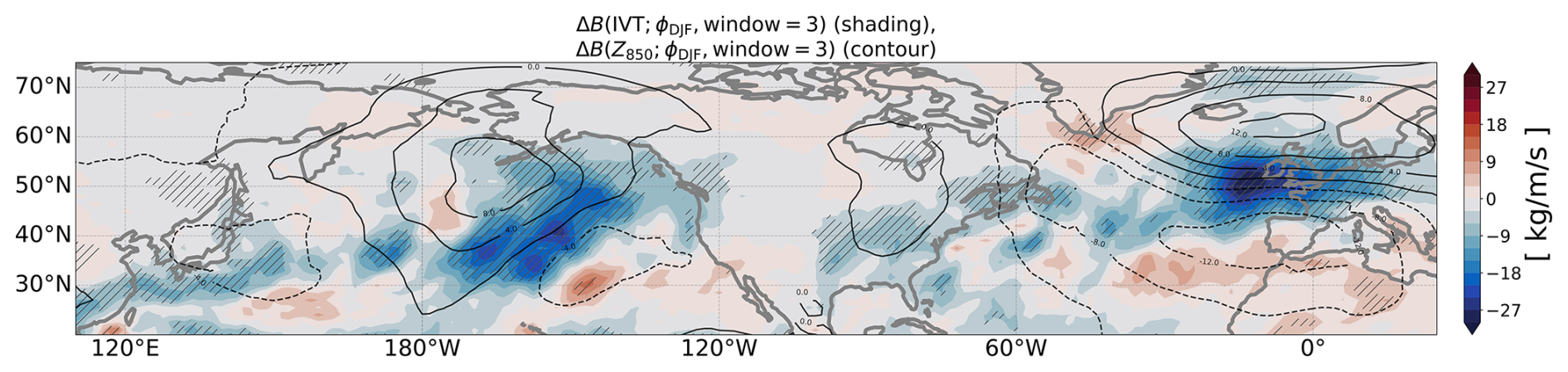
Figure 2 Bias changes ΔB of the integrated vapor transport (IVT, shading) and 850 hPa geopotential height Z₈₅₀ (contours, spacing is 2 m, and contours with negative values are dashed) computed from Global Ensemble Forecast System (GEPS) version 5 (GEPS5) to GEPS version 6 (GEPS6) during December–January–February of the first three pentads in hindcast years 1998–2017. The hatched area means the IVT anomalies pass the significance test of a p-value of 0.1.

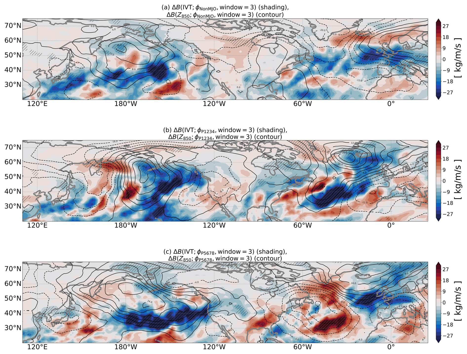
Figure 3 Bias changes ΔB of the integrated water vapor (IVT, shading) and 850 hPa geopotential height Z₈₅₀ (contours, spacing is 2 m, and contours with negative values are dashed) from Global Ensemble Forecast System (GEPS) version 5 (GEPS5) to GEPS version 6 (GEPS6) of the third pentad p=3 in different start time groups in hindcast years 1998–2017 during December–January–February. (a) Non-MJO group. (b) P1234 group. (c) P5678 group. The hatched area means the IVT bias change passes the significance test of a p-value of 0.1.

The shape of the IVT bias depends on the MJO. Figure 3a–c show the composite bias changes of IVT (shading) and Z₈₅₀ (contour) grouped by MJO-inactive, MJO phases 1–4, and MJO phases 5–8 as defined in Sect. 2.4. The weakened Aleutian Low remains in the middle of the North Pacific, such that the weakened Pacific IVT is consistently oriented southwest–northeast. In contrast, the Icelandic Low and Atlantic Subtropical High weakening is spatially more variable, such that the Atlantic IVT pattern is less consistent across MJO groups.

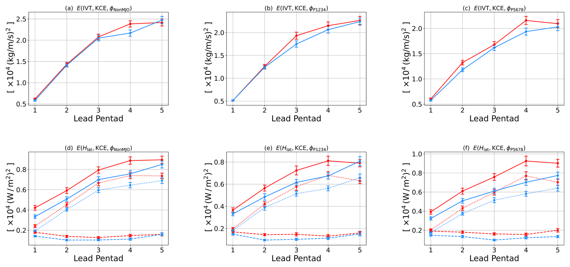
Figure 4 Bias variance E analysis of quantities as a function of pentads 1–5 computed from Global Ensemble Prediction System (GEPS) version 5 (GEPS5, red) to GEPS version 6 (GEPS6, blue) over the Kuroshio Current Extension (KCE) region for Non-MJO group (a, d), P1234 group (b, e), and P5678 group (c, f). (a–c) Integrated vapor transport (IVT). (d–f) Latent heat flux (H_lat). For H_lat (d–f), the decomposition of E into mean ($\stackrel{\mathrm{‾}}{E}$, dashed) and patterned ($\stackrel{\mathrm{̃}}{E}$, dotted) variances is added. The whiskers represent the standard error.

Over the North Pacific, the IVT forecast is improved when the MJO is active. Figure 4a–c show the composited bias variance of IVT over the Kuroshio Current region. The first 3 pentads of non-MJO cases do not show significant differences, while the MJO phases 1–4 and 5–8 show better IVT forecasts starting in pentads 3 and 2, respectively. The lag of the improvement in MJO phases 1–4 by one pentad is reasonable because MJO convection is located over the Indian Ocean during phases 1–4, and it takes some time for the MJO convection to propagate into the Pacific.

Examining the latent heat flux H_lat, we find that both the mean and patterned bias variances of H_lat are improved regardless of MJO phase (Fig. 4d–f). This does not mean latent heat flux is irrelevant. Rather, it shows that more accurate heat fluxes can positively impact the forecast during a certain window of opportunity, which in our case is MJO phases 5–8. We are also aware that, because using the dynamical ocean model also gives better MJO forecasts (Lin et al., 2019), the exact improvement due to local air–sea interaction will be more easily studied using a regional coupled model.

For the North Atlantic, we do not find a similar improvement that depends on MJO phase (not shown).

3.3 Coupling to a Dynamical Ocean Model Improves Latent Heat Fluxes

We use bias variances as functions of lead pentads over the Kuroshio Current Extension and Gulf Stream regions to assess the benefit of using a dynamical ocean model over persistent SST anomaly, as shown in Fig. 5a–j. In the Kuroshio Current Extension region, GEPS6 performs better than GEPS5 in terms of the mean SST variance, but has poorer performance in patterned SST variance (Fig. 5a). The patterned SST variance hindcast gradually reaches the mean ERA5 SST variance 0.60±0.16 K (zonally detrended and area weighted variance, years 1998–2017 DJF). By comparison, we find that the SST initialization choice in GEPS6 reduces the mean but increases the patterned bias variances of SST, which together increase about 0.05 K². In the Gulf Stream regions, the initialization in GEPS6 adds 0.5 K² of SST patterned bias variance, and the mean bias variance does not change significantly. The SST patterned bias variance introduced can be due to lack of eddies because GEPS6 initializes the ocean with the monthly mean ORAP5 dataset.

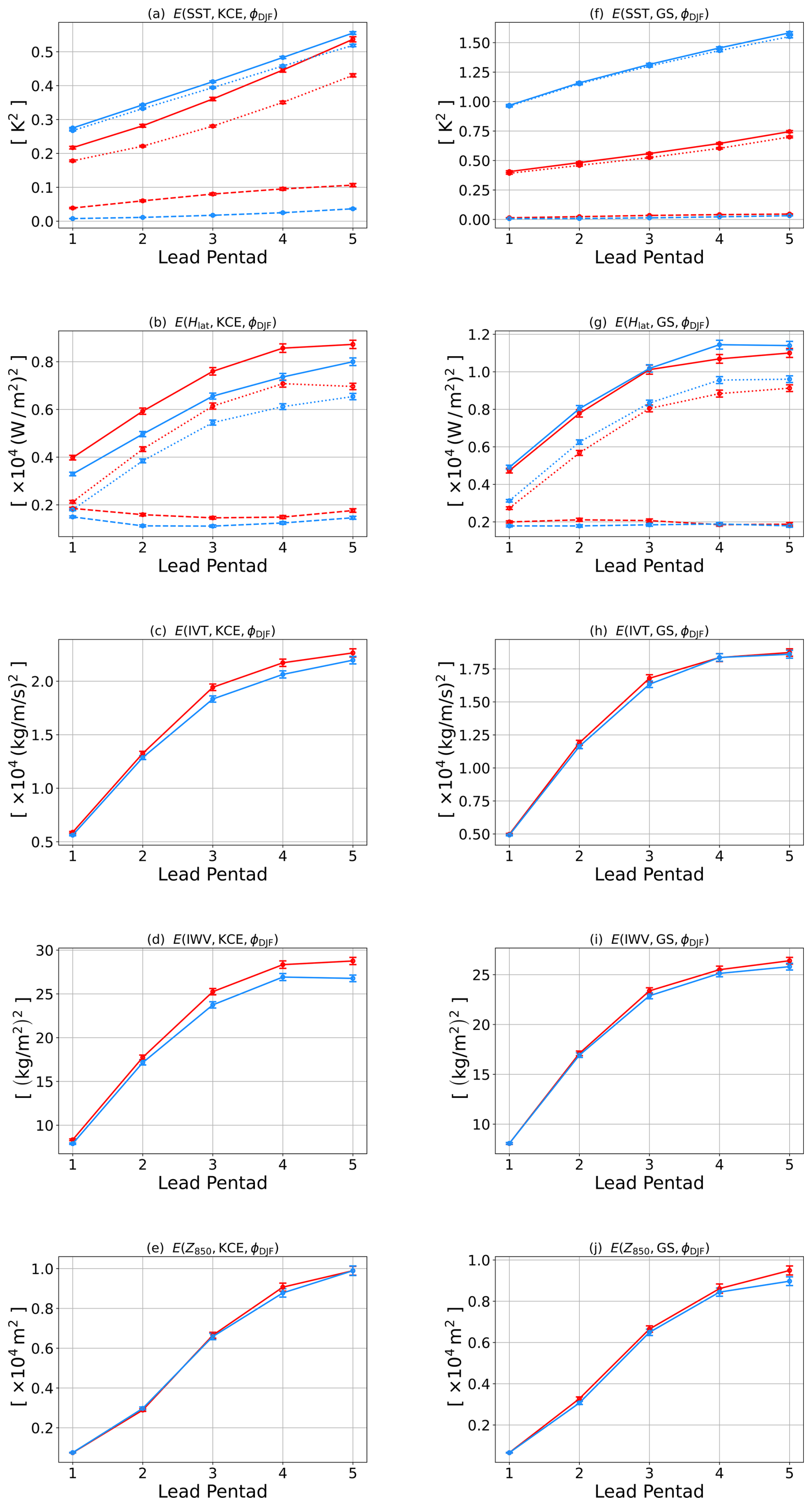
Figure 5 Bias variance E analysis of quantities as a function of pentads 1–5 computed from Global Ensemble Prediction System (GEPS) version 5 (GEPS5, red) to GEPS version 6 (GEPS6, blue) during December–January–February of the first three pentads in hindcast years 1998–2017. (a, f) Sea surface temperature (SST). (b, g) Latent heat flux (H_lat. (c, h) Integrated vapor transport (IVT). (d, i) Integrated water vapor (IWV). (e, j) 850 hPa geopotential height Z₈₅₀. For SST (a, f) and H_lat (b, g), the decomposition of E into mean ($\stackrel{\mathrm{‾}}{E}$, dashed) and patterned ($\stackrel{\mathrm{̃}}{E}$, dotted) variances are added. Panels (a)–(e) are for the Kuroshio Current Extension (KCE) region, and panels (f)–(j) are for Gulf Stream (GS) region. The whiskers represent the standard error.

Despite the initial SST error introduced, in the Kuroshio Current Extension region the latent heat flux H_lat, GEPS6 outperforms GEPS5 in both mean and patterned variances (Fig. 5b), and the bias variance E of GEPS6 is 10 %–20 % smaller than that of GEPS5, as noted in the previous section. Because GEPS6 produces a less accurate SST but a better latent heat flux, this contrast highlights the importance of two-way coupling in correctly predicting air–sea fluxes, especially those associated with extra-tropical cyclones (Kobashi et al., 2019; Hsu et al., 2024). The improvement of H_lat during MJO active phase, subsequently leads to a better integrated water vapor (IWV, defined as $\mathrm{IWV}=g^{-\mathrm{1}}{\int }_{\mathrm{200}\mathrm{hPa}}^{\mathrm{1000}\mathrm{hPa}}q\mathrm{d}p$) and therefore better IVT hindcast in GEPS6 (Fig. 5c–d). In contrast, GEPS6 does not produce a better Z₈₅₀ hindcast than GEPS5 (Fig. 5e).

In the Gulf Stream region, GEPS6 simulates a lower mean variance of SST bias in the first three pentads. However, because GEPS6 simulates a northward-shifted Gulf Stream, there is a strong patterned variance of SST bias (Fig. 5f). This signal propagates into patterned variance of H_lat bias (Fig. 5g), resulting in little or no improvement in IWV and IVT (Fig. 5h–i). Moreover, similar to the Kuroshio Current Extension region, we do not see a notable difference in Z₈₅₀ (Fig. 5j).

3.4 What Causes the Continuation of Aleutian Low Weakening?

In this section, the goal is to understand the physical mechanisms that cause changes in the Aleutian Low. From Fig. 3a–c, we know that the weakening bias is first triggered by less than 0.3 K colder SST over the North Pacific in GEPS6 relative to GEPS5, and the weakening continues regardless of MJO phases. This is an indication that local air–sea coupling is an important driver for the Aleutian Low weakening.

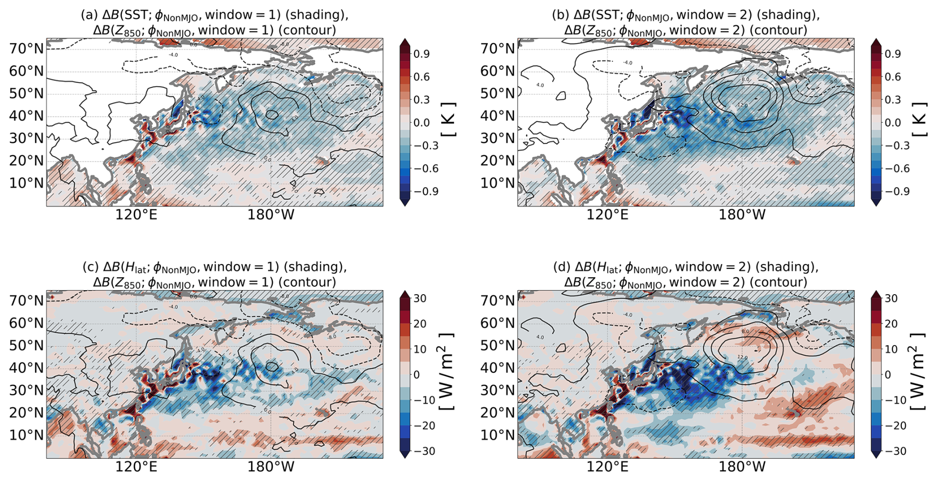
Figure 6 Bias change ΔB of the sea surface temperature (SST), upward latent heat flux (H_lat), and the 850 hPa geopotential height Z₈₅₀ from Global Ensemble Forecast System (GEPS) version 5 (GEPS5) to GEPS version 6 (GEPS6) during Madden–Julian–Oscillation (MJO) inactive start time (ϕ_NonMJO) of the first two p=1, 2 in hindcast years 1998–2017. (a) The shading is the $\mathrm{\Delta }{B}_{\mathrm{SST}}({\mathit{\varphi }}_{\mathrm{NonMJO}},p=\mathrm{1})$. The contours are the $\mathrm{\Delta }{B}_{Z_{\mathrm{850}}}({\mathit{\varphi }}_{\mathrm{NonMJO}},p=\mathrm{1})$. The hatched areas are the location where $\mathrm{\Delta }{B}_{H_{\mathrm{SST}}}$ passes the significance test of a p-value of 0.15. (b) Same as panel (a) but for p=2. (c) Same as panel (a) but the shading and dotted-hatch are for the $\mathrm{\Delta }{B}_{H_{\mathrm{lat}}}({\mathit{\varphi }}_{\mathrm{NonMJO}},p=\mathrm{1})$. (d) Same as panel (c) but for p=2.

To remove the MJO influence, we examine the response of Z₈₅₀ and latent heat fluxes H_lat composited with non-MJO groups. In the absence of MJO, the Aleutian Low weakens in GEPS6 relative to GEPS5 during pentads 1–2 (contours in Fig. 6a–d). The SST bias change between 30–60° N is −0.2 K in the first pentad due to difference in SST initialization strategy, and potential issues in model resolution (see Sect. 4). This results in a reduction in H_lat (Fig. 6c shading), causing a weaker cyclogenesis such that the Z₈₅₀ is positively biased.

The Aleutian Low experiences a positive feedback loop where its initial weakening leads to further intensification of this weakening, primarily through interactions between circulation and H_lat. In particular, notice that the magnitude of the reduction in H_lat is larger at the southern flank of the Z₈₅₀ anomaly because its anomalous circulation blows against the mean westerlies (Fig. 6c). As previously demonstrated, the reduction of H_lat leads to a weaker Aleutian Low, resulting in stronger anomalous circulation in the next pentad (Fig. 6d). This mechanism is a positive feedback.

Given differences in the initial SST and the use of a global model, further isolation of this feedback is beyond the ability of the present framework. Nonetheless, the results underscore the potential of future regional modeling studies to more directly quantify the strength of the feedback.

4 Discussion: The Role of Kuroshio Current Extension and the Gulf Stream

Both the Kuroshio Current Extension and the Gulf Stream are eddy-rich regions where mesoscale (200 km and less) SST fronts modify the near-surface atmospheric convergence, curl, and thus air–sea fluxes in the marine atmosphere boundary layer (MABL) (Masunaga et al., 2015; Bishop et al., 2017; Seo et al., 2023; Renault et al., 2024). In addition to modulating air–sea interaction, the resolution of the ocean model also impacts western boundary currents. While the resolution of the 0.25° ocean model used in GEPS6 is sufficient to resolve mesoscale eddies (0.5–2° or 50–200 km) (An et al., 2023), Chassignet and Xu (2017) suggest that much finer resolution (less than $\mathrm{1}/\mathrm{12}$° or 8 km) is required to resolve the smaller eddies to obtain the observed magnitude of eddy kinetic energy in boundary currents, and therefore adequately resolve the positions of boundary separation and eastward turns for both the Kuroshio and Gulf Stream currents.

Our results show that the SST bias over the Kuroshio Current Extension leads to an Aleutian Low positive feedback response, implying that better Aleutian Low prediction can be achieved through optimizing the initialization. Improving these factors will lead to better forecasts of the North Pacific jet and IVT, both of which are indicators for AR activities (Winters, 2021; Higgins et al., 2024).

The role of the Gulf Stream is less clear. While its persistent impact on Z₈₅₀ is visible (Fig. 1d–f), and the major atmospheric response over the Atlantic Ocean is immediately downstream of the Gulf Stream, the response does not emerge until the second pentad. This aligns with the reanalysis studies showing that the Gulf Stream variability leads the North Atlantic Oscillation (NAO) by a month through its strong temperature gradient that impacts the boundary processes during cyclogenesis (Parfitt and Kwon, 2020; Chakravorty et al., 2024; Alsepan and Parfitt, 2025). Given its strong bias but ambiguous downstream influence, regional modeling with various domain sizes, or global modeling experiments that vary configuration only in the Gulf Stream, is needed to isolate the impact.

5 Conclusion

This study, using 20 years of hindcast data from ECCC's GEPS5 and GEPS6 alongside ERA5 reanalysis, demonstrates the impact of using a dynamical ocean model on medium-range wintertime forecasts over the North Pacific and North Atlantic.

The analysis of hindcast bias shows that the air–sea coupling results in a weaker Aleutian Low, Icelandic Low, and Atlantic Subtropical High within 15 d, leading to a weaker IVT over the northeastern Pacific and Atlantic. We also notice how the biased Aleutian Low due to difference in SST initial conditions can subsequently impact the Icelandic Low via teleconnection, as is consistent with reanalysis studies (Honda et al., 2001; Li et al., 2024). Furthermore, the MJO phase can influence the resulting spatial distribution of IVT difference, suggesting its importance in tropical–extratropical interactions.

We investigated the cause of the continuation of Aleutian Low weakening after the first pentad. The initialization and dynamical ocean coupling simulates a colder SST centered on the Kuroshio Current Extension within the first pentad, which reduces the latent heat flux. This leads to weaker cyclogenesis and thus a weaker Aleutian Low. The anomalous circulation that blows against the westerlies over the Kuroshio Current Extension further reduces the latent fluxes, creating a positive feedback loop that reinforces the initial bias.

When evaluating the bias variance, we find that the coupled model produces a slight degradation in SST hindcast, but a significant reduction of 10 %–20 % in latent heat flux bias variance over the Kuroshio Current Extension compared to the uncoupled model, likely associated with the frontal activities that are spatially inhomogeneous. The improvement in latent heat flux explains the better IWV and thus the IVT hindcast. The IVT improvement is also more significant when the MJO is active. In the Gulf Stream, the northward shift bias is too strong such that the latent heat fluxes, and thus IWV and IVT, are not improved. This basin-dependent behavior implies different limiting factors in the North Pacific and Gulf Stream regions. In the North Pacific, the quality of the initial SST is high enough that the improvement can be made through better air–sea interactions, such as higher-order turbulent mixing schemes or the inclusion of a wave model (Sauvage et al., 2023). In the North Atlantic, the initial Gulf Stream SST bias remains large such that improving the air–sea interaction will not yield significantly improved forecasts, unless better air–sea interaction leads to a higher quality of initial assimilated SST.

Finally, this research highlights two potential future directions. First, regional simulations over the North Atlantic can be performed to isolate the influence of the Atlantic from the Pacific (Cassou, 2008). Second, there is a need for more physical understanding of how two-way coupling produces better air–sea fluxes, in which case the simple stochastic model such as Barsugli and Battisti (1998) can be inspirational.

This potentially can mitigate the SST error along the Kuroshio Current Extension and the Gulf Stream that can tangibly force the atmosphere through modifying air–sea fluxes (Seo et al., 2023).