A spread-versus-error framework to reliably quantify the potential for subseasonal windows of forecast opportunity

Mid-latitude forecast skill at subseasonal timescales often depends on “windows of opportunity” that may be opened by slowly varying modes such as ENSO, the MJO or stratospheric variability. Most previous work has focused on the predictability of ensemble-mean states, with less attention paid to the reliability of such forecasts and how it relates to ensemble spread, which directly reflects intrinsic forecast uncertainty. Here, we introduce a spread-versus-error framework based on the Spread-Reliability Slope (SRS) to quantify whether fluctuations in ensemble spread provide reliable information about variations in forecast error. Using ECMWF S2S forecasts and ERA5 reanalysis data, aided by idealised toy-model experiments, we show that spread reliability is controlled by at least three intertwined factors: (1) sampling error, (2) the magnitude of physically driven spread variability and (3) model fidelity in representing that variability. Regions such as northern Europe, the mid-east Pacific, and the tropical west Pacific exhibit robustly high SRS values (i.e. reliable spread fluctuations) for 50-member ensembles, consistent with robust spread modulation by slowly varying teleconnections. In contrast, areas like eastern Canada show very low SRS (little or no spread reliability), even for 100-member ensembles, reflecting limited low-frequency modulation of forecast uncertainty. We further demonstrate two practical implications: (i) a simple variance rescaling yields a post-processed “corrected spread” that enforces reliability and may help to bridge ensemble output with user needs; and (ii) time averaging effectively boosts ensemble size, allowing even 10-member ensembles to achieve reliability of spread fluctuations comparable to larger ensembles. Finally, we discuss possible links to the signal-to-noise paradox and emphasize that adequate representation of ensemble spread variability is crucial for exploiting subseasonal windows of opportunity.

1 Introduction

Atmospheric predictability at subseasonal timescales (about 2 weeks to 2 months) varies strongly with region and season. At these timescales probabilistic (i.e. ensemble) forecasts are vital as uncertainty is generally large and forecast skill may arise due to both an ensemble mean signature and reduced ensemble spread. Previous work has identified that during certain periods, and over particular regions, intrinsic forecast uncertainty can be anomalously low, indeed enabling higher forecast skill at these longer leadtimes (Mariotti et al., 2020). Such periods with reduced uncertainty are often referred to as “windows of forecast opportunity”. These windows typically arise due to the influence of slowly varying atmospheric modes (Vitart and Robertson, 2018) that can be considered to exert a quasi-external influence on the region of interest. For northern hemispheric mid-latitude forecasts these slowly varying modes include those of tropical origin such as the El Nino-Southern Oscillation (ENSO;  Johnson et al., 2014) and the Madden-Julian Oscillation (MJO;  Baggett et al., 2017), and of upper atmospheric origin such as stratospheric polar vortex variability (Baldwin et al., 2003). Importantly, windows of opportunity can only occur if intrinsic forecast uncertainty varies substantially across different forecast situations. Regions with little variability in forecast uncertainty cannot exhibit such windows, because uncertainty remains close to its climatological value at all times. We refer to such situations as a low potential to exhibit windows of opportunity. The “potential for windows of opportunity” therefore refers to the variability of ensemble spread, that is, the capacity of the atmosphere to occasionally enter low-uncertainty states. Most studies investigating windows of opportunity analyse changes in the skill of the ensemble-mean forecast (e.g. Vitart and Robertson, 2018; Robertson et al., 2020). However, probabilistic forecasts aim to accurately capture not only the mean of the probability distribution (the prediction of the actual value), but also higher moments such as the ensemble spread (the prediction of the uncertainty). Quantitative analyses of this intrinsic forecast uncertainty, as measured explicitly by the ensemble spread or variance of a forecast, are comparatively rare, and our study attempts to help fill this gap.

Previous work established that this forecast uncertainty can be highly flow-dependent (Spaeth et al., 2024b). Hence, mid-latitude tropospheric forecast spread may indeed be substantially modulated by slowly varying tropical or stratospheric teleconnections. Specifically, Spaeth et al. (2024a) recently demonstrated that the northern European subseasonal forecast uncertainty of 1000 hPa geopotential height (z1000), as directly reflected in ensemble spread, is reduced after breakdowns of the stratospheric polar vortex due to equatorward shifts of the North Atlantic storm track. Such slowly varying teleconnections and associated intrinsic predictability changes can have significant non-local impacts on ensemble spread as well. For instance, Spaeth et al. (2024a) also showed how ENSO can modulate ensemble spread in the northern Pacific. Identifying and quantifying the potential of the atmosphere to exhibit windows of opportunity might therefore be beneficial for both improving forecasts and gaining insights into the underlying dynamics of the system.

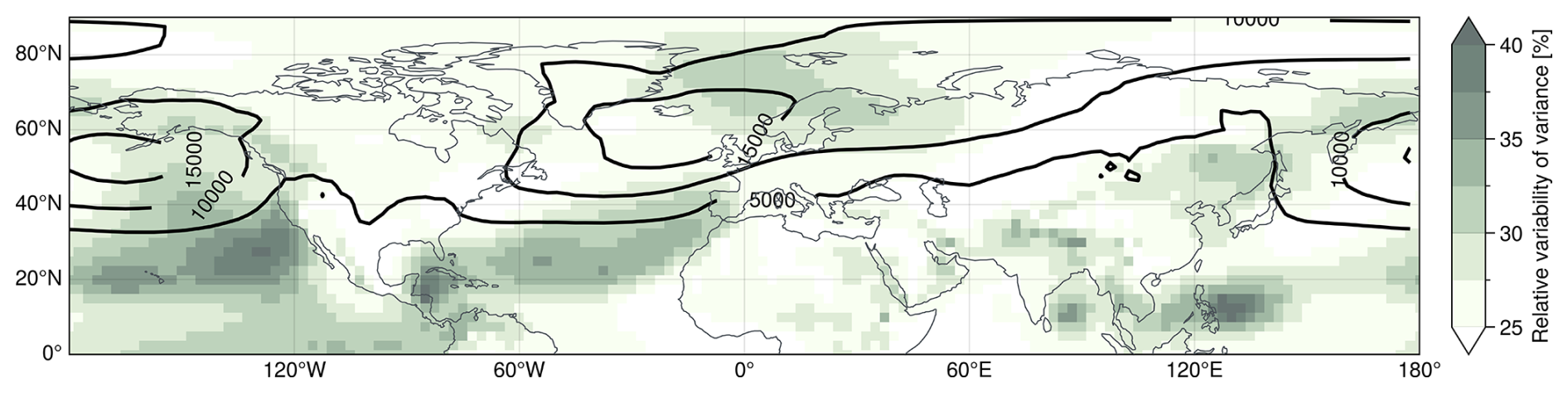
Figure 1 Intrinsic variability of subseasonal z1000 forecasts in the northern hemisphere for 50-member ensembles initialized in DJF (see Sect. 2 for information on the dataset). Contour lines show DJF climatological mean spread [in m²] computed from daily ensemble variance values averaged over subseasonal leadtimes (14 to 46 d). Note that computing the figure based on weekly averaged data leads to overall similar large-scale structures. The shading shows relative variability in subseasonal spread, measured as standard deviation of the ensemble variance across all DJF forecast initializations and subseasonal leadtimes, normalised by the climatological average variance. Areas with large relative spread variability suggest that spread computed from individual forecasts provide added value over a fixed spread climatology, potentially identifying windows of opportunity.

Figure 1 illustrates the climatology of ensemble spread in subseasonal winter-time forecasts of z1000 over the northern hemisphere. In addition to the spread itself, it highlights regions exhibiting substantial variability in spread (i.e., areas occasionally associated with relatively low or high spread). Such areas with large relative spread variability suggest that ensemble spread computed from individual forecasts provides added value over a fixed spread climatology. Only in such regions can forecast uncertainty occasionally be anomalously low, implying a potential for windows of forecast opportunity to exist. In contrast, regions with little spread variability lack this potential, as forecast uncertainty remains close to its climatological value. Prominent regions of high relative spread variability include the northern Euro-Atlantic sector, the subtropical Atlantic, and the tropical and subtropical Pacific.

In the extratropics, enhanced z1000 variability often appears on the flanks of the climatological maxima in spread over the North Pacific and North Atlantic. This pattern is consistent with meridional shifts of the storm tracks and associated jets, such that locations on the flanks alternately lie within or outside the high-spread belt, while the core persistently contains high-spread and therefore exhibits smaller relative variability. Such flank variability can be further amplified by remote influences via atmospheric teleconnections, for example through stratospheric downward influence or tropical-extratropical coupling. At the same time, several highlighted regions, particularly in the tropical Pacific, likely reflect more local signatures of slowly varying modes such as ENSO or the MJO. Some of these slow modes and teleconnections have been explicitly linked to enhanced forecast skill at subseasonal to seasonal timescales (e.g., Johnson et al., 2014; Baggett et al., 2017). Given this significant spatial and temporal variability in ensemble spread, an important question arises: Are these variations in ensemble spread within a model forecast reliable indicators of the uncertainty within the physical system?

Ensemble forecasting is a widely used approach to quantify forecast uncertainty and exploit windows of opportunity. The fundamental assumption of ensemble forecasting is that ensemble members and observations are statistically exchangeable, i.e., indistinguishable. From this assumption, it follows that the spread of the ensemble (i.e. the variability across members) reflects the intrinsic forecast uncertainty or, in other words, the expected error of the ensemble mean. Specifically, in an ideal, infinitely large, and statistically reliable ensemble system, the ensemble's variance across members should, on average, equal the squared error of the ensemble-mean forecast (Fortin et al., 2014). If this is the case, we would consider the spread to be a reliable estimate of the forecast error.

However, real-world ensemble systems rarely achieve perfect reliability. While comprehensive diagnostics of spread-reliability are limited at subseasonal lead times, ensemble spread has been shown to lack reliability at other lead times. At short to medium lead times (up to 2 weeks), model forecasts typically show under-dispersion, where the error exceeds the error predicted by the ensemble spread (e.g. Lakatos et al., 2023). At seasonal to decadal lead times, on the other hand, atmospheric ensemble forecasts seem to be, on average, relatively reliable in their prediction of uncertainty (Weisheimer et al., 2019). However, while the average ensemble spread might be a good indicator of forecast error, misrepresentations of short-term fluctuations in spread may still exist. In the following, we investigate whether such misrepresentations can limit the ability of ensembles to identify genuine windows of opportunity, since periods with low predicted uncertainty might underestimate actual errors. Ensuring that variability in ensemble spread realistically reflects variability in forecast error is therefore critical for reliable decision support.

Numerous studies have examined how the spread-error relationship varies regionally and among forecast variables, especially during Northern Hemisphere winter (DJF). Results indicate that regional variations in ensemble reliability are linked to the intrinsic variability of the ensemble spread itself. For example, Scherrer et al. (2004) analysed different uncertainty metrics for forecasts over Europe, finding generally reliable spread-error relationships. However, most previous analyses, including that of Scherrer et al. (2004), have been restricted to medium-range forecasts (up to approximately two weeks). At these shorter leadtimes, forecast dynamics strongly depend on specific synoptic conditions, with ensemble spread variations largely reflecting the error growth dynamics initiated by initial condition perturbations (Selz, 2019; Selz et al., 2022), rather than mostly describing the intrinsic predictability of the underlying physical system, which is the focus of this study.

Reliability diagrams have also been widely used in other contexts. One common approach involves comparing forecasted versus observed probabilities of specific weather events (Bröcker and Smith, 2007; Weisheimer and Palmer, 2014). Such reliability diagrams typically assess the overall calibration of ensemble predictions but do not explicitly focus on the spatio-temporal variability of ensemble spread as done in this study. Another frequent application is the evaluation of initial perturbation schemes during short to medium-range forecasts. These analyses typically use reliability diagrams of spread and error primarily to identify under- or over-dispersion at early forecast stages, subsequently guiding adjustments to initial perturbation magnitudes (Leutbecher and Palmer, 2008; Giggins and Gottwald, 2019). In contrast, the framework applied in this study emphasises the intrinsic atmospheric uncertainty and flow-dependent variations in ensemble spread and associated forecast error specifically at subseasonal lead times rather than the average or climatological level of forecast skill (although it can also highlight model errors in representing these processes).

Throughout this paper, we distinguish between windows of forecast opportunity and the potential for windows of forecast opportunity. A window of forecast opportunity refers to a specific forecast situation characterised by anomalously low intrinsic forecast uncertainty, as reflected by reduced ensemble spread. The potential for windows of opportunity refers to the variability of forecast uncertainty across different forecast situations. Only regions or variables with substantial spread variability can occasionally realise low-spread states and thus exhibit windows of opportunity. However, only if the ensemble spread of a forecast is a reliable measure of forecast error do these windows actually represent opportunities with reduced forecast error.

The structure of the present manuscript is as follows: Sect. 2 describes the datasets and ensemble configurations. Section 3 introduces the spread-error reliability metric and identifies potential processes modifying reliability. Section 4 uses an idealized toy model to isolate if and how these processes affect reliability curves. Section 5 then applies the reliability diagnostics to operational subseasonal forecasts and assesses regional spread forecast skill. Finally, Sect. 6 summarizes the main findings and their implications for atmospheric dynamics and model development.

2 Data and numerical models

2.1 Re-analysis data

We use the ERA5 re-analysis dataset (Hersbach et al., 2020) of the European Centre for Medium range Weather Forecasts (ECMWF) as the representation of the atmospheric state between 1 December 2015 and 30 April 2025. In particular, we use daily snapshots of geopotential height at 1000 hPa (z1000) at 00:00 UTC and daily mean 2-metre temperature (t2m) computed from 3-hourly data. All outputs are analysed on a 2.5° × 2.5° regular grid covering the entire northern hemisphere.

2.2 Subseasonal ensemble forecasts

This study uses ensemble forecasts provided by ECMWF as part of the S2S Prediction Project (Vitart et al., 2017). In particular, we use real-time forecasts initialised during boreal winter months December to February for the period from late 2015 to early 2025. The inherent horizontal model resolution is roughly 30 km, but we analyse outputs for z1000 and t2m on the same 2.5° grid as used for the re-analysis (see Sect. 2.1). Model output is given for 46 d after initialisation, although most of our analyses will focus on subseasonal leadtimes of 14 to 46 d. Consistent with the ERA5-data, we analyse daily instantaneous snapshots of z1000 and daily mean t2m.

Forecasts are initialised twice a week (Monday and Thursday) as 50-member ensembles before 27 June 2023 and daily as 100-member ensembles afterwards. Note that in this study we do not use the “unperturbed control member” of each forecast, as it is not strictly statistically indistinguishable from the perturbed members.

To study the effect of ensemble size and forecast uncertainty we create a set of smaller ensembles by subsampling the original 100-member and 50-member ensembles. The subsampling is done by simply splitting, for example, the 100-member ensembles into two 50-member ensembles (by taking members 1 to 50 and 51 to 100, respectively). We use the same approach to subsample the 100-member and 50-member ensembles into 10 and 5 ensembles with 10 members each, respectively. The combined set of original and subsampled ensembles gives us a total of 181 forecasts with 100 members, 568 forecasts with 50 members and 2840 forecasts with 10 members. Note hereby that these sets of forecasts combine different model versions, as the operationally used S2S model gets updated regularly. The subsampling approach mixes, for example, “original” 50-member ensembles using version CY47R2 with “subsampled” 50-member ensembles using version CY49R1. However, for the purposes of this study we assume the representation of atmospheric uncertainty to vary little between different model versions, as previous studies indicate that ensemble spread characteristics remain broadly consistent across model designs. For example, Leutbecher et al. (2024) reported only small changes (a few percent) in subseasonal forecast spread when changing the stochastic perturbation scheme in the IFS model. In addition, a qualitative comparison with an independent CNRM ensemble (see model details below) yields similar large-scale patterns in spread reliability, further supporting this assumption (see Sect. 6).

As representation of model spread in this study, we use the unbiased sample variance over ensemble members at a given time. Model errors are further given as squared error, i.e., the squared difference of the ensemble mean and the corresponding re-analysis value. The main focus of this study is then the relation of spread and squared error. Using sufficiently large sample averages, these two metrics should be equal to each other if the model accurately represents the inherent uncertainty of atmospheric evolution (as discussed in Sects. 1 and 4). Note that, in contrast to some other studies, we will not analyse the relationship of spread and mean squared error given by temporal averages, but rather as averages over different atmospheric states associated with a given uncertainty. We do so by averaging over groups of forecast ensembles and/or time steps with the same ensemble variance. Forecast situations with low spread are then expected to also show, on average, low squared error.

However, for finite ensemble sizes, sampling errors can lead to deviations between the estimated ensemble spread and the underlying forecast uncertainty. In individual forecast situations, this can result in cases where relatively low estimated spread is associated with comparatively large forecast error (or the other way round), not because spread is an inherently poor predictor, but because the spread is underestimated due to sampling variability. This will in general weaken the expected linear relationship of spread and error and reduce the slope of spread-error curves. What constitutes a “small” ensemble size in this context is relative and depends on the strength of flow-dependent variability and the number of available forecast cases; while 50-member ensembles are large by operational standards, sampling effects are nevertheless present and become increasingly important for smaller ensembles. These aspects are further discussed in Sects. 3 and 4.

In addition to the IFS ensemble forecasts, we use a second, independent ensemble dataset produced with the CNRM subseasonal forecast system for a qualitative comparison of spread reliability patterns (see Sect. 6). The CNRM data are used solely to assess the robustness of large-scale features identified in the IFS and are not analysed in the same level of detail. We analyse CNRM daily model data output on a 0.5° grid for DJF-initialisations between end of 2016 and early 2025, with one initialisation per week. For CNRM geopotential height is only available on the 925 hPa surface (z925), necessarily resulting in deviations from results based on the IFS z1000 data, which we assume to be sufficiently small for our comparisons. CNRM ensembles have 50 members before December 2020, and 24 members afterwards. The 50-member ensembles are sub-sampled, as explained above, to further obtain 24- and 10-member ensembles.

3 Methodology of reliability analyses

In the present study, we analyse fluctuations in the spread of subseasonal ensemble forecasts to investigate the flow-dependent variability of intrinsic forecast uncertainty. For a reliable model, those fluctuations in ensemble spread are expected to translate into corresponding fluctuations in mean squared error. We emphasise that our framework focuses on spread variability and the associated potential for windows of forecast opportunity, whereas other measures of forecast skill or accuracy may depend on additional factors beyond the scope of this study. In particular, we present a framework to investigate the potential of the atmosphere to develop prolonged periods of reduced spread, i.e., potential windows of opportunity. We then use this framework to quantify the ability of the model to accurately predict such periods given limited ensemble sizes, model misrepresentation and other common sources of errors. Note that, our framework can, in principle, also be used to identify periods with anomalously high ensemble spread (which one might analogously refer to as “walls of adversity”).

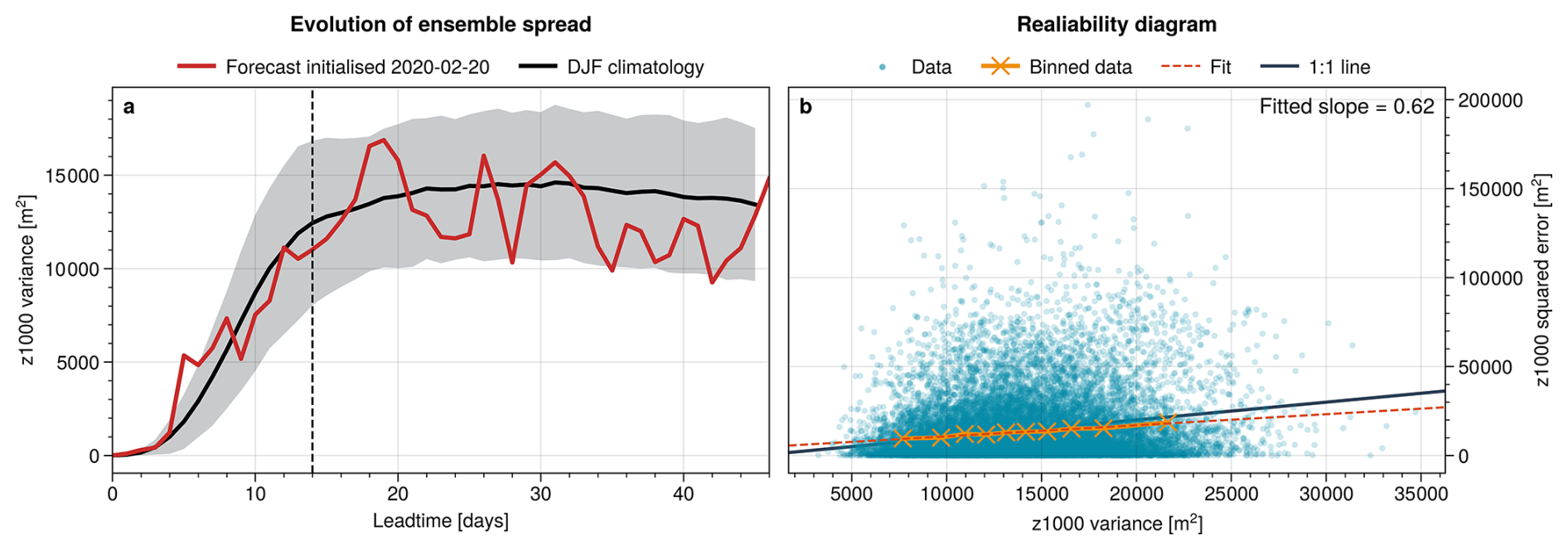
Figure 2 Visualisation of ensemble spread and spread-error relation at an example point in northern Europe (60° N/15° E) based on 50-member ensembles. (a) Evolution of spread in terms of ensemble variance as function of leadtime. Shown is the DJF climatological mean with shading indicating 1 standard deviation and an example forecast initialised on 20 February 2020. Vertical dashed line indicates 14 d of leadtime. (b) Spread-error relation with blue dots showing z1000 variance and squared error for every subseasonal leadtime (days 14–46) and all 568 ensembles in the dataset. Orange crosses show the means of 10 bins in variance direction, spaced to contain equal number of points each. The dashed line shows a linear fit through the bin means, with slope indicated in the top right. Black solid line shows the 1:1 line for reference.

Figure 2a illustrates how the ensemble spread evolves with leadtime in subseasonal z1000 forecasts for a selected point in northern Europe. Shown are the “climatological” spread evolution as averaged over all forecasts in DJF, as well as one specific example of the forecast initialised on 20 February 2020. For short leadtimes (up to about day 14), the climatological spread increases substantially until it converges to a roughly constant value at subseasonal leadtimes (after 14 d), marking the transition from the rapid initial error-growth phase to a quasi-saturated spread level. The spread of the example forecast essentially follows the climatological evolution, but shows a large degree of day-to-day variability around it. In the following, we therefore focus on leadtimes 14–46 d. Restricting the analysis to this window avoids a trivial spread-error relationship arising purely from their common dependence on lead time. A sensitivity analysis using leadtimes 28–46 showed overall consistent large-scale patterns in SRS (not shown), indicating that residual lead-time trends do not dominate our results.

In general, the spread of an ensemble forecast should be a measure of the forecast uncertainty (cf. Sect. 1). We can therefore assess the reliability of predicted fluctuations in spread by comparing them to the associated forecast errors. Note that, following Fortin et al. (2014), the expected squared error of the ensemble mean equals the ensemble variance only when scaled by a factor of $M/(M+\mathrm{1})$ for ensemble size M. This factor essentially results from a reduction in degrees of freedom when computing the error based on an empirically estimated ensemble mean. In this study we consistently apply this “unbiasing” correction when computing the error. However, for simplicity, we will refer to this unbiased error as error (without the prefix “unbiased”) throughout the paper.

Figure 2b shows how the z1000 squared error behaves in relation to the z1000 ensemble variance for the point in northern Europe. Plotted are the squared error and spread at every subseasonal leadtime (days 14–46) within all 50-member forecasts in our dataset (see Sect. 2.2), we hence capture fluctuations on daily to inter-annual time scales.

The forecast errors shown in Fig. 2 are computed based on a single observed evolution of the atmosphere and hence the resulting spread-error scatter plot shows a very disperse distribution. For a given value of ensemble variance, and under the assumption that the ensemble members are normally distributed and the model is perfect, the corresponding squared error follows a χ²-distribution (e.g. Wilks, 2011). For a reliable forecast, the mean of that error distribution should equal the associated variance value.

Indeed, when binning cases with similar spread in Fig. 2, the bin-means collapse onto an almost linear relationship in good agreement with the 1:1 curve. Here we divide the distribution into 10 bins with equal number of samples in each bin. To quantify the agreement with the 1:1 line, we fit a linear function through the bin-means and extract the slope of that fit. We refer to this slope as the Spread-Reliability Slope (SRS), which represents the reliability of fluctuations in the spread of a forecast at a given location. The spread-error relationship diagnosed here is inherently statistical and holds only on average, so substantial scatter between individual spread-error pairs is expected. In addition, extreme spread values are comparatively rare, so that the raw scatter may visually suggest relatively low errors at the highest spread values; this reflects sampling imbalance and the skewness of the error distribution rather than a breakdown of the monotonic increase of mean error with spread. If the spread was perfectly reliable, we would have SRS=1, as all bin-means would collapse onto the 1:1 line and the ensemble variance would perfectly represent the average forecast uncertainty. Any deviation of the SRS from 1 indicates a lack of reliability of the spread. In the case shown, we have SRS=0.62 and hence we consider the fluctuations in spread of the forecast fairly reliable (further comparison values will be discussed below).

The spread-error scatter in Fig. 2b is based on daily values. For subseasonal forecasting, time-averaged quantities such as weekly means are often more closely aligned with the low-frequency modes that provide predictability. However, daily ensemble spread is occasionally available and inspected in ensemble forecasts or operational products, for example in the form of spaghetti plots or ensemble evolution diagrams. Further, using daily values provides a useful baseline diagnostic: it allows us to assess whether day-to-day spread fluctuations in the ensemble output already contain meaningful information about forecast error. In addition, daily values provide substantially better sampling of the spread-error distribution than time-averaged quantities.

While daily values can exhibit substantial pointwise scatter, the SRS is derived from averages over many spread-error pairs and is therefore not sensitive to the noise of individual points. Daily spread and error values within a given forecast are temporally autocorrelated, which reduces the effective number of statistically independent samples. As discussed in Sect. 5, the SRS is primarily controlled by differences between forecasts rather than day-to-day fluctuations within a forecast, so temporal autocorrelation mainly affects sampling uncertainty rather than the existence of a systematic spread-error relationship.

Computing the SRS metric from long-term time-averaged data (e.g. weekly means) suppresses high-frequency, potentially spurious variability but reduces the number of available spread-error pairs. We therefore view daily and time-averaged analyses as complementary. As shown in Sect. 5, SRS patterns based on time-averaged spread remain qualitatively consistent and are often enhanced, indicating that the main conclusions are robust while also highlighting the benefit of temporal aggregation.

We can now apply the same methodology to analyse the reliability of different locations by extracting the SRS metric of the associated ensemble forecasts at these locations. Figure 3 shows that the reliability of subseasonal forecast spread varies substantially across the northern hemisphere. For example, northern Europe has SRS values robustly exceeding 0.6, while the SRS in parts of eastern Canada is statistically not different from zero. In fact, different pronounced regions of high SRS can clearly be identified, e.g., in the northern Atlantic, the mid-east Pacific, the tropical west Pacific or the Gulf of Mexico. Over the North Atlantic, the spatial structure exhibits a pronounced north-south contrast within the sector associated with the North Atlantic Oscillation (NAO), with comparatively higher SRS values over the northern centre of action than over the southern centre. As discussed in Sect. 6, the relatively high reliability of spread in these regions is likely due to a strong influence of slowly varying modes of atmospheric variability driven by different teleconnections.

Regions of high SRS mark locations where ensemble spread fluctuations reliably track fluctuations in intrinsic forecast uncertainty and associated forecast errors, indicating that slowly varying teleconnections can modulate forecast uncertainty and thereby create the potential for windows of forecast opportunity. Our framework is not designed to assess the average or climatological level of forecast skill in a given region. Instead, it diagnoses whether forecast error varies in a flow-dependent manner and whether such variations are reliably captured by ensemble spread. In such regions, periods of reduced spread correspond to reduced forecast error, while other periods exhibit increased error, implying a potential for both enhanced and degraded forecast skill rather than uniformly high skill.

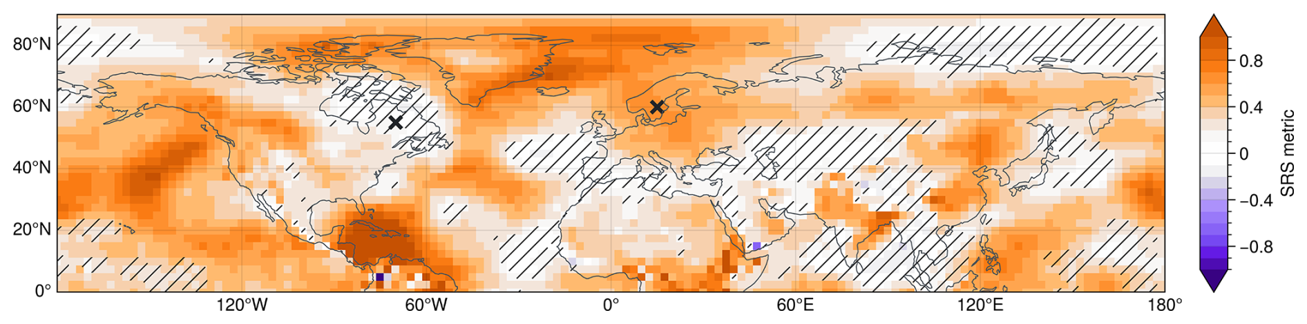
Figure 3 SRS metric computed as the slope of the linear fit to the z1000 spread-error curve at each point in the northern hemisphere. Shown are results for 50-member ensembles. Hatched areas indicate regions where the SRS metric (derived from the regression of bin-mean error on spread) is not statistically different from zero at the 99 % confidence level. Crosses indicate two example locations (eastern Canada at 55° N$/$70° W and northern Europe at 60° N$/$15° E) further analysed below.

For the remainder of this study, we investigate the mechanisms and processes that can lead to the pronounced spatial structures in SRS shown in Fig. 3. We use a combination of toy-model experiments and comprehensive perfect-model approaches to examine how intrinsic variability and sampling-related misrepresentation of ensemble spread influence the slope of the spread-error relationship.

Our framework does not require the ensemble mean to be perfectly represented. Instead, it focuses on how fluctuations in ensemble spread relate to fluctuations in forecast error when diagnostics are constructed from averages over many forecast cases. For finite ensemble sizes, individual forecasts can exhibit sampling uncertainty in both estimated spread and associated forecast error. However, because the SRS is derived from averages over many forecasts within variance bins, sampling-induced uncertainties in forecast error are largely random across cases and therefore mostly cancel out in the bin mean. Deviations of the SRS from unity instead arise when sampling effects and other limitations reduce the contrast between low- and high-uncertainty forecast situations. These mechanisms are further illustrated and discussed using toy-model experiments in Sect. 4.2. The potential role of ensemble-mean biases and other model deficiencies is discussed separately in Sect. 6.

We identified four major mechanisms that can modify the reliability of a spread forecast and lead to SRS≠1, although other mechanisms might exist:

• Sampling error: random misrepresentation of ensemble spread due to small ensemble sizes

• Natural variability: modification of the sampling error effect due to variability of spread in the physical system

• Model error: misrepresentation of the variability of spread in the model

• Under-representation of states: Insufficient sampling of initial conditions producing forecasts with a given spread value

In Sect. 4, we start by using a statistical toy model to isolate each of these four mechanisms and study their specific effects on spread-error curves and the SRS individually. We then analyse these mechanisms and their impacts on spread reliability in operational forecast systems in Sect. 5. This two-step approach enables us to develop an intuitive understanding of the individual processes before quantifying their effects in more complex, real-world forecast settings, where the mechanisms typically interact and are challenging to disentangle.

4 Reliability curves studied in a toy model

4.1 Details of the toy model

In this section, we seek to develop an intuitive understanding of different mechanisms that can modify the reliability of spread in a forecast in terms of the slope of associated spread-error curves (i.e., the SRS metric). To study how individual mechanisms can affect the SRS, we use a statistical toy model that generates synthetic forecast-observation pairs with controlled properties.

We start by generating C ensemble forecast cases, divided equally into five groups. Each forecast comprises M ensemble members. The forecast value $x_{\mathrm{F},\mathrm{m},\mathrm{c}}$ (the subscript F denotes “forecast”) for case “c” $\in \mathit{\{}\mathrm{1},\mathrm{\dots },C\mathit{\}}$ and ensemble member “m” $\in \mathit{\{}\mathrm{1},\mathrm{\dots },M\mathit{\}}$ is randomly sampled from a normal distribution with zero mean and a standard deviation σ_F,c, i.e., $x_{\mathrm{F},\mathrm{m},\mathrm{c}}\sim \mathcal{N}(\mathrm{0},{\mathit{\sigma }}_{\mathrm{F},\mathrm{c}}^{\mathrm{2}})$. Here, we can vary σ_F,c for different forecast cases, which allows us to mimic natural variability in the spread of the underlying physical system. Situations where σ_F,c is small, for example, then represent periods with low intrinsic uncertainty (i.e. windows of opportunity). By varying other parameters (like M, C or σ_F,c) we can sample other experimental setups that mimic different characteristics of the forecasting model or underlying physical system. The values used for the different parameters are given below.

For each forecast, we then generate an observation x_O,c (the subscript “O” denotes “observation”) by sampling from a normal distribution with zero mean and a standard deviation σ_O,c, i.e., $(x_{\mathrm{O},\mathrm{c}}\sim \mathcal{N}(\mathrm{0},{\mathit{\sigma }}_{\mathrm{O},\mathrm{c}}^{\mathrm{2}}\left)\right)$.

Given the ensemble members $x_{\mathrm{F},\mathrm{m},\mathrm{c}}$ and observations x_O,c corresponding to forecast case “c”, the ensemble mean is then computed as

$$\begin{array}{}\text{(1)}& {\stackrel{\mathrm{‾}}{x}}_{\mathrm{F},\mathrm{c}}={\displaystyle \frac{\mathrm{1}}{M}}\sum _{m=\mathrm{1}}^M{x}_{\mathrm{F},\mathrm{m},\mathrm{c}},\end{array}$$

the ensemble variance (spread) as

$$\begin{array}{}\text{(2)}& s_{\mathrm{F},\mathrm{c}}^{\mathrm{2}}={\displaystyle \frac{\mathrm{1}}{M-\mathrm{1}}}\sum _{m=\mathrm{1}}^M{\left(x_{\mathrm{F},\mathrm{m},\mathrm{c}}-{\stackrel{\mathrm{‾}}{x}}_{\mathrm{F},\mathrm{m}}\right)}^{\mathrm{2}},\end{array}$$

and the squared error (SE) with respect to the observation as

$$\begin{array}{}\text{(3)}& {\mathrm{SE}}_{\mathrm{c}}={\left({\stackrel{\mathrm{‾}}{x}}_{\mathrm{F},\mathrm{c}}-x_{\mathrm{O},\mathrm{c}}\right)}^{\mathrm{2}}.\end{array}$$

Note that for a given observation-forecast pair, the ensemble variance $s_{\mathrm{F},\mathrm{c}}^{\mathrm{2}}$ provides an unbiased estimate of the underlying forecast variance ${\mathit{\sigma }}_{\mathrm{F},\mathrm{c}}^{\mathrm{2}}$. However, the accuracy of this estimate improves with increasing ensemble size.

Our modelling strategy within the toy model includes a reference experiment and different perturbation experiments, where we vary individual parameters to simulate changes to the model and physical system and isolate their effect on the resulting spread error curve. The reference case is supposed to represent an “ideal case”, associated with a spread-error slope of exactly one (SRS=1). The parameter setup for this reference case is given in Table 1a.

Table 1 Overview of toy model experiment configurations, with the top row describing the reference experiment. Here, M denotes the ensemble size, C the number of forecast-observation pairs, σ_O the standard deviation of the observations, and σ_F the standard deviation of the forecast ensemble members. The two experiments mimicking few verification dates (g/h) are initialised with different random seeds, but use otherwise equal parameters. Parameters deviating from our “standard set-up” (labeled Ideal spread-error relationship) are shown in bold, for easier identification of the sensitivity studied in respective experiments.

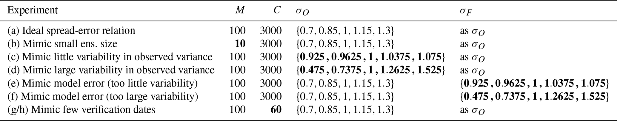
Here, we choose a large ensemble size of M=100, which corresponds to the ensemble size of the latest operational subseasonal forecast system at ECMWF. Lower values of M then model smaller ensembles. We further choose a case sample size of C=3000, considerably larger than the number of 100-member forecasts analysed in this study (which is 181 for 100-member ensembles; see Sect. 2.2). Modifying C allows us to model the effect of this reduced sample size of cases. Within the reference experiment, we then vary the variability of observed spread σ_O,c by choosing values from the set $S=\mathit{\{}\mathrm{0.7},\mathrm{0.85},\mathrm{1.0},\mathrm{1.15},\mathrm{1.3}\mathit{\}}$. Specifically, the first $C/\mathrm{5}$ forecasts use ${\mathit{\sigma }}_{\mathrm{O},\mathrm{c}}=\mathrm{0.7}$, the next $C/\mathrm{5}$ forecasts use ${\mathit{\sigma }}_{\mathrm{O},\mathrm{c}}=\mathrm{0.85}$, and so on, with the final $C/\mathrm{5}$ forecasts using ${\mathit{\sigma }}_{\mathrm{O},\mathrm{c}}=\mathrm{1.3}$. Our qualitative conclusions are not sensitive to the precise distribution of the set S, but it can modify some aspects of the shape of the spread-error curves. However, we run experiments with a reduced or increased range of values in S to mimic underlying physical systems with low or large variability in their intrinsic uncertainty, respectively. These different physical systems could represent different spatial locations or periods in different seasons. Additionally, we can choose the forecast distribution (i.e., σ_F,c) to exactly match the observed distribution σ_O,c (which simulates a perfect model), or follow different distributions (which simulates model error). A summary of the different experiments and their associated parameter combinations is given in Table 1.

4.2 Sensitivities of spread-error curves in the toy model

Figure 4a shows the spread-error curve for the reference toy model experiment. This reference experiment uses a large ensemble size (M=100) with good sampling (C=3000) and a correct model representation of the forecast distribution (${\mathit{\sigma }}_{\mathrm{O},\mathrm{c}}={\mathit{\sigma }}_{\mathrm{F},\mathrm{c}}$). Therefore, the spread-error curve lies almost exactly on the 1:1 line, as expected, with spread-reliability-slope of SRS=0.99.

If we reduce the ensemble size to 10 members (Fig. 4b), the spread-error curves becomes more shallow and hence the SRS reduces as random differences between the ensemble sample variance ($s_{\mathrm{F},\mathrm{c}}^{\mathrm{2}}$) and the underlying forecast population variance (${\mathit{\sigma }}_{\mathrm{F},\mathrm{c}}^{\mathrm{2}}$) become larger.

The reduction of the SRS in this case is not caused by changes in the underlying predictable signal, but by sampling uncertainty associated with the finite ensemble size. At the level of individual forecasts, sampling noise affects both the estimated ensemble spread and the associated forecast error, leading to substantial scatter in the spread-error relationship. However, the SRS is not diagnosed from individual spread-error pairs, but from averages over many forecasts grouped by similar estimated spread. Sampling-induced fluctuations in forecast error are largely random across cases and therefore mostly cancel out in the bin means, such that uncertainty in the error does not systematically bias the mean spread–error relationship within a bin.

A systematic effect instead arises from sampling noise in the spread estimate itself. For small ensemble sizes, random under- and overestimation of the ensemble sample variance $s_{\mathrm{F},\mathrm{c}}^{\mathrm{2}}$ leads to a redistribution of forecasts across variance bins. Consequently, bins with high estimated spread include some forecasts with lower true uncertainty, while bins with low estimated spread include some forecasts with higher true uncertainty. This misclassification systematically reduces the contrast between low- and high-spread bins, flattening the spread-error curve and leading to a reduced SRS.

Note that a similar argument applies if SRS is obtained from a linear regression of the full spread-error distribution, rather than via explicit variance binning, as the reduction in slope is likewise driven by sampling-induced distortion of the spread-error contrast. Random fluctuations in forecast error would, in this case, primarily increase the scatter around the regression and the associated uncertainty of the fit, while leaving the best-fit slope, and thus the inferred SRS, largely unchanged.

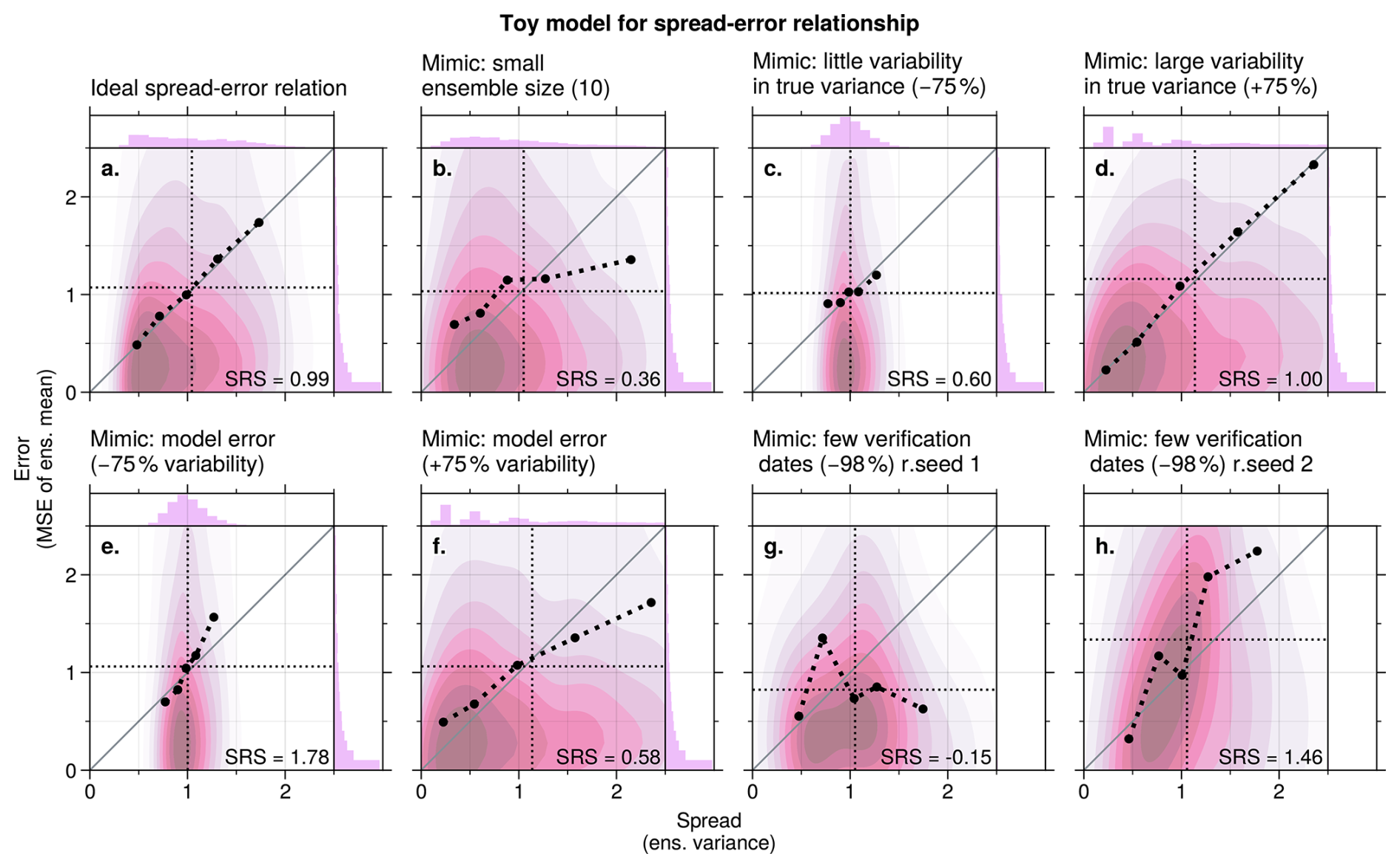
Figure 4 Toy model experiments illustrating the spread–error relationship (ensemble variance vs. mean squared error of the ensemble mean). Pink shading shows the 2D distribution of individual spread–error pairs. Black dots indicate the average spread and error within each bin. For visual guidance, these bin means are connected with thick dashed black lines. Note that the pink shading highlights where samples are most frequent, while the black dots show bin means and can therefore lie in low-density regions, particularly in the distribution tails. Thin black dotted lines indicate the overall mean spread (vertical) and error (horizontal). The solid grey diagonal line represents the 1:1 relationship. The spread-reliability-slope (SRS) is indicated for each case.

An equivalent geometric perspective on the SRS reduction is the following. Consider that in a system with perfectly reliable spread (in which ${\mathit{\sigma }}_{\mathrm{O},\mathrm{c}}^{\mathrm{2}}$ = ${\mathit{\sigma }}_{\mathrm{F},\mathrm{c}}^{\mathrm{2}}$), the forecasts with the largest true variance, ${\mathit{\sigma }}_{\mathrm{O},\mathrm{c}}^{\mathrm{2}}$, should lie on the 1:1 line when plotting variance against the case-averaged squared error. However, since neither ${\mathit{\sigma }}_{\mathrm{O},\mathrm{c}}^{\mathrm{2}}$ nor ${\mathit{\sigma }}_{\mathrm{F},\mathrm{c}}^{\mathrm{2}}$ are known in practice, we use the ensemble sample variance $s_{\mathrm{F},\mathrm{c}}^{\mathrm{2}}$ as an estimate. While this estimate is perfect in each single case in an infinitely large ensemble, it is subject to sampling noise when the ensemble size is finite. As a result, averages over cases with the highest spread values (i.e., those with the largest ensemble spread $s_{\mathrm{F},\mathrm{c}}^{\mathrm{2}}$) will not only include cases with genuinely large forecast variance ${\mathit{\sigma }}_{\mathrm{F},\mathrm{c}}^{\mathrm{2}}$, but also cases with smaller forecast variance that appear inflated due to sampling fluctuations. These forecasts misclassified as high-spread tend to underestimate their expected error compared to what their spread suggests, thus lowering the average error for that variance value and pulling it below the 1:1 line. The reverse happens for averages over cases with the lowest spread values: it may include forecasts with higher true variance that were misclassified due to sampling variability. These cases have overestimated errors compared to what the spread suggests and increase the average error in the bin, pulling it above the 1:1 line. The net effect is a systematic reduction of the SRS. Note that bins in the centre of the spread range will usually include forecasts with both over- and underestimated spread. For those bins the biases due to sampling effects mostly cancel out.

This behaviour is consistent with ensemble sampling theory, which provides insight into why forecasts with few members often misrepresent variability in spread. With small ensemble sizes M, the sample variance becomes noisy (high “variance of the variance”), and individual forecasts may, by chance, fail to sample extreme outcomes, causing the actual error to exceed the predicted spread. Increasing M reduces this sampling error, as the standard error of the spread estimate decreases proportional to $\mathrm{1}/\sqrt{M}$ (cf. Tempest et al., 2023). In general, larger ensembles are therefore required to obtain a stable spread–error relationship, especially for higher-order moments such as the ensemble variance.

The impact of sampling noise due to finite ensemble size also depends on the intrinsic variability of the true uncertainty, ${\mathit{\sigma }}_{\mathrm{O},\mathrm{c}}^{\mathrm{2}}$, which is determined by the characteristics of the underlying physical system. If ${\mathit{\sigma }}_{\mathrm{O},\mathrm{c}}^{\mathrm{2}}$ varies strongly across cases (i.e., if the range $\left[{min}_{\mathrm{c}}{\mathit{\sigma }}_{\mathrm{O},\mathrm{c}}^{\mathrm{2}},{max}_{\mathrm{c}}{\mathit{\sigma }}_{\mathrm{O},\mathrm{c}}^{\mathrm{2}}\right]$ is large) then the relative effect of sampling noise becomes less significant. In such cases, the differences between ${\mathit{\sigma }}_{\mathrm{F},\mathrm{c}}^{\mathrm{2}}$ and its noisy estimate $s_{\mathrm{F},\mathrm{c}}^{\mathrm{2}}$ are small compared to the variability in ${\mathit{\sigma }}_{\mathrm{F},\mathrm{c}}^{\mathrm{2}}$ itself. As a result, even with a finite ensemble size, the binning of forecasts by spread is more robust, and the spread-skill relationship appears less distorted. This effect is illustrated in Fig. 4c, d. In panel c, σ_F,c varies within a narrow range (0.925 to 1.075), while in Fig. 4d it spans a much broader range (0.475 to 1.525). The comparison shows that larger variability in spread of the physical system improves the clarity of the spread-skill relationship under finite ensemble conditions, mitigating the SRS reduction due to sampling error.

In addition to sampling error and natural variability in spread, model biases in how intrinsic uncertainty responds to physical drivers can also affect the spread-error relationship. For instance, anomalies in ensemble spread may be systematically too small if the model responds too weakly to teleconnection patterns. The opposite would be true if the model responds too strongly to teleconnections. In our toy model, such biases can be mimicked by choosing different values for the variance of observed (σ_F,c) and modelled (σ_O,c) distributions. Figure 4e and f show experiments where the model over- or underestimates the anomalies in spread. Such a misrepresentation of the spread leads to a stretching or compression of the distribution in variance-direction. Analogous to the effect discussed with regards to sampling error, this will affect the slope of the spread-error curve and alter the SRS. In general, an over-estimation of spread variability (so ${\mathit{\sigma }}_{\mathrm{F},\mathrm{c}}/{\mathit{\sigma }}_{\mathrm{O},\mathrm{c}}>\mathrm{1}$ and a stretching in variance direction) will lead to SRS<1, while an under-estimation of spread variability will do the opposite and lead to SRS>1. Note that here we are discussing over- and under-estimation of the variations in spread, and not an overall over- or under-estimation of the mean spread (which may or may not be accurate on average).

Next we analyse the effect of a limited number of cases, i.e., few forecast-observation pairs (small C). This will in general lead to a violation of the underlying equality between errors and spread (see Sect. 3) and introduce random deviations of the spread-error curve from the 1:1 line. Since these deviations are unsystematic, they can randomly lead to increases or decreases of the SRS. A system with an under-representation of cases can therefore, in principle, produce an SRS larger than 1 (see Fig. 4h), smaller than 1 or even smaller than 0 (see Fig. 4g). Note that in situations with small C the SRS could take very large or very small (or even negative) values despite the underlying ensemble forecast having many members and no model error.

The toy model presented in this section allowed us to study the effects of different mechanisms on the spread-error curves and the SRS in an isolated manner. While some of these effects are systematic and always increase or decrease the SRS (e.g. the ensemble size effect), others are unsystematic (e.g. associated with number of forecast cases). A forecasting system will typically suffer from multiple error sources. This can lead to a superposition of the corresponding effects and hence SRS values that either deviate strongly from one for multiple reasons, or SRS values close to 1 despite major error sources due to cancellation. The next section analyses the reliability of spread forecasts in subseasonal ensembles by trying to disentangle the different mechanisms and studying their potential importance individually.

5 Reliability of operational forecasts

5.1 Sampling error due to ensemble size

Various mechanisms can affect the reliability of spread forecasts and lead to deviations of the SRS from unity, as shown within the toy model in Sect. 4. This section goes through the list of individual mechanisms and analyses their importance within subseasonal ensemble forecasts of the real atmosphere.

We start by analysing the effect of sampling error on the SRS. Figure 5 shows the reliability of z1000 spread within the northern hemisphere for three different ensemble sizes. It can be seen that the SRS generally increases with ensemble size. While 10-member ensembles show poor spread reliability almost throughout the entire hemisphere (SRS close to zero), 50-member ensembles exhibit substantially more reliable spread in various regions (e.g. northern Europe, eastern Asia, western North America or around the Gulf of Mexico), with SRS closer to 1. We see further SRS improvements in many of these regions, when increasing the ensemble size to 100 members. However, for 100-member ensembles we find regions with SRS larger 1 or negative SRS. This is likely due to the limited number of 100-member ensembles available and reflects an under-representation of atmospheric evolutions in the system (cf. Fig. 4c).

Figure 5 SRS metric computed as the slope of the z1000 spread-error curve in the northern Hemisphere. As Fig. 3 but for forecast of different ensemble size (10, 50 and 100 members). Note that panel (b) is identical to Fig. 3.

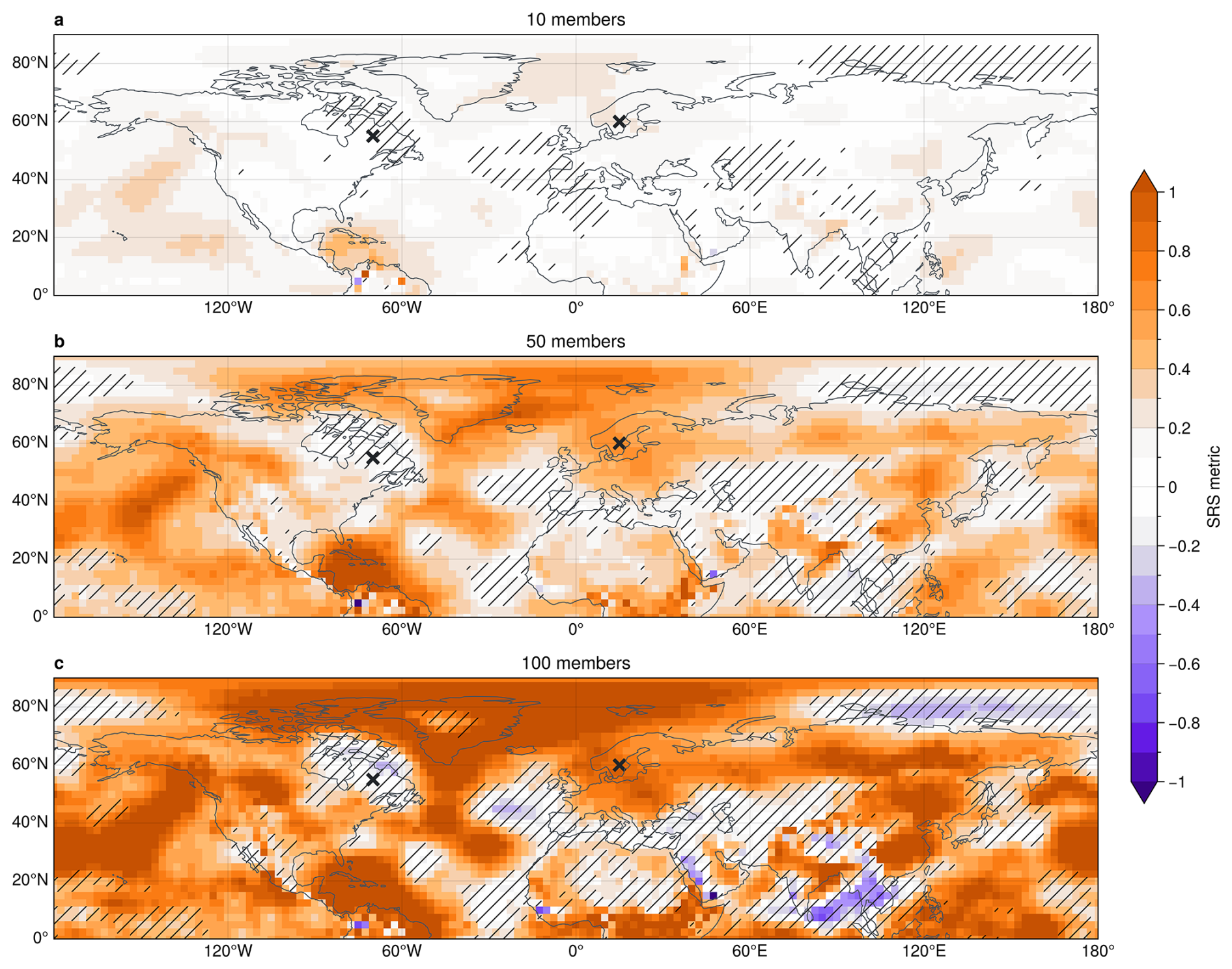
Although 50 and 100 member ensembles show generally reliable spread in many regions, other regions do not exhibit visible improvements with increasing ensemble size. A pronounced region in eastern Canada, for example, is associated with a slope robustly close to zero. Other effects therefore seem to play an important role here, reducing the reliability of spread fluctuations in the forecasts. In the next section, we show that a lack of variability within the physical system is a major contributor to the lack of reliability in these regions.

5.2 Intrinsic variability of the physical system

As shown within the toy model in Sect. 4, the intrinsic variability of spread within the underlying physical system can have a strong effect on the spread-error curve and the SRS, due to modification of the sampling error effect. To illustrate and further quantify the effect of variability in spread we contrast two example locations, one in eastern Canada (55° N$/$70° W) and one in northern Europe (60° N$/$15° E). While northern Europe shows strong improvement of SRS with increasing ensemble size and very reliable spread forecasts for 50- and 100-member ensembles, eastern Canada shows low SRS for all ensemble sizes (Fig. 5).

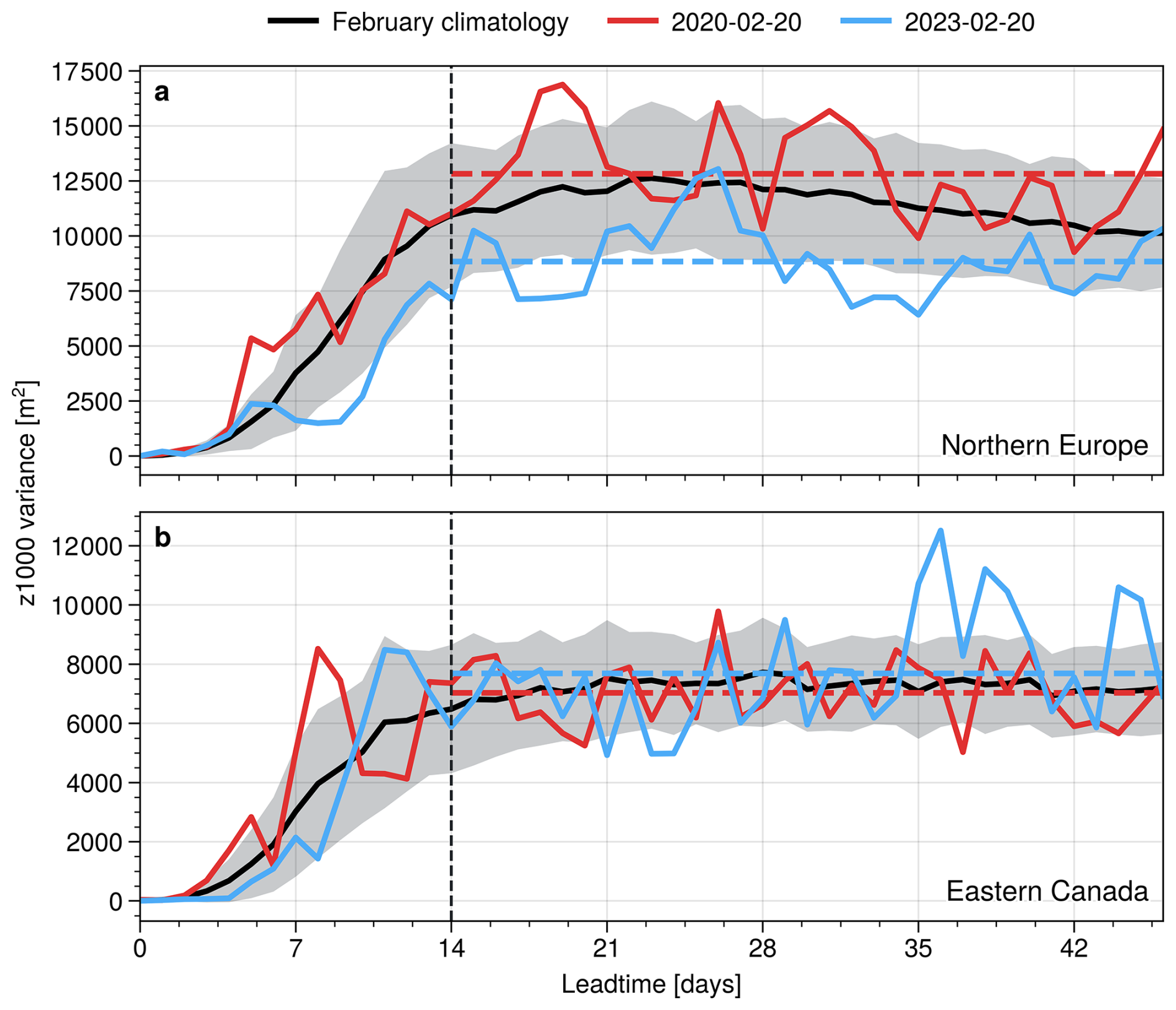
Figure 6 Evolution of leadtime-dependent ensemble variance in (a) Northern Europe at 60° N$/$15° E and (b) eastern Canada at 55° N$/$70° W. Thick black line shows the climatology for February as average over all February initialisations, with shading indicating one standard deviation around the mean. Red and blue lines show variance evolution of example forecasts with 50 members initialised on 20 February of the years 2020 and 2023, respectively. Dashed horizontal lines show the average over the respective variance between days 14 and 46. Vertical dashed line indicated day 14 as visual aid.

Figure 6 indicates the variability of ensemble spread at these two points. It can be seen that the climatological day-to-day variability in spread is generally larger in northern Europe (Fig. 5a) than eastern Canada (Fig. 5b). The difference in variability between two points in time and at a given location mostly comes from slowly varying modes of atmospheric variability that affect the spread, as discussed in the following. To distinguish between slow and fast modes of variability, we will decompose changes in spread within and across forecasts into two components. These components are defined formally below using the ensemble variance as a function of forecast case and lead time.

Let s²(c,t) denote the ensemble variance of forecast c at lead time t. We use the notation 〈⋅〉_t and 〈⋅〉_c to denote averages over lead times and forecasts, respectively. The specific lead-time range over which the temporal averages are taken can be chosen as appropriate for the application.

• Inter-variability: This quantifies differences in the mean spread between different forecasts and is defined as the variance across forecasts of the time-averaged ensemble variance, $s_{\mathrm{inter}}^{\mathrm{2}}=\frac{\mathrm{1}}{C-\mathrm{1}}{\sum }_{c=\mathrm{1}}^C{\left(\langle s^{\mathrm{2}}{\rangle }_t-{〈\langle s^{\mathrm{2}}{\rangle }_t〉}_c\right)}^{\mathrm{2}}$. It therefore characterises variability in spread associated with differences between forecast cases, for example due to slowly varying modes of variability.

• Intra-variability: This quantifies day-to-day fluctuations of the spread within individual forecasts and is defined as the forecast-mean of the temporal variance of the ensemble variance, $s_{\mathrm{intra}}^{\mathrm{2}}={〈\frac{\mathrm{1}}{N_t-\mathrm{1}}{\sum }_t{\left(s^{\mathrm{2}}-\langle s^{\mathrm{2}}{\rangle }_t\right)}^{\mathrm{2}}〉}_c$, where N_t denotes the number of lead times included in the temporal average. This quantity therefore captures the contribution of faster, intra-forecast variability to the evolution of ensemble spread.

The concept of inter- and intra-variability is visualised in Fig. 6 by two example forecasts. Both forecasts are initialised on 20 February, but in two different years: 2020 and 2023. It can be seen that in northern Europe, the two forecasts are associated with substantially different spread at subseasonal leadtimes, suggesting large inter-variability of the spread in this region. The inter-variability, i.e., the difference between subseasonally averaged variances of the two forecasts, is of the same order as the intra-variability, i.e., the day-to-day fluctuations in spread. In eastern Canada, on the other hand, the two example forecasts do not essentially differ in their subseasonal mean variance, and only show deviations from each other due to intra-variability (i.e., day-to-day variations).

Figure 7 displays the dependence of inter- and intra-variability on underlying ensemble size at the two points in eastern Canada and northern Europe. This allows us to study the two variability components more systematically. Figure 7 further shows how the two components should depend on sample size if variations were entirely due to sampling error and not due to physical drivers. Under this assumption, the theoretical sampling error scaling is taken to decrease with ensemble size M as $\mathrm{1}/\sqrt{M}$, with the reference value estimated from the corresponding variability obtained for 10-member ensembles. It can be seen that in northern Europe the inter-variability converges clearly to a value of about 3000 m² for large ensembles and does not follow the theoretical line of sampling errors. This suggests a pronounced inter-variability in the physical system, which is well-sampled with ensemble sizes exceeding about 50 members. Intra variability, however, follows almost perfectly the theoretical line of sampling errors, suggesting that day-to-day variability is entirely spurious. In general, this leads to a gradual increase of the ratio of inter- over intra-variability, which exceeds one at an ensemble size of about 50.

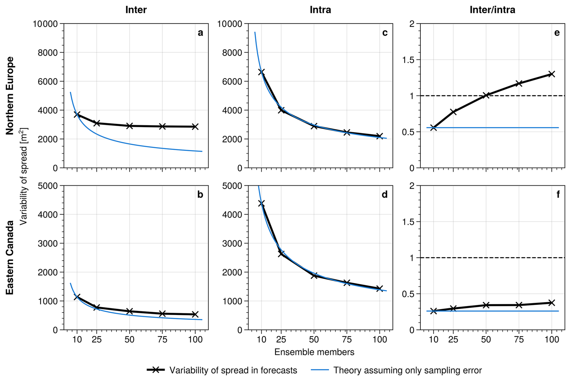
Figure 7 Average (a, b) inter and (c, d) intra variability at subseasonal leadtimes computed for forecasts with varying ensemble size. (e) and (f) show the ratio of inter-over-intra variability. Top row (a, c, e) shows a point in northern Europe at 60° N$/$15° E and bottom row (b, d, f) shows a point in eastern Canada at 55° N$/$70° W. Blue thin lines indicate theoretical dependency of variability components on ensemble size M, computed as value for 10 member ensembles divided by $\sqrt{M}$. Dashed horizontal lines in (e) and (f) indicate a ratio of 1.

For the point in eastern Canada, both inter- and intra-variability follow rather closely the line of sampling error theory. Even for 100 member ensembles the inter-variability has not converged yet and seems to be substantially affected by sampling errors. This leads to generally low inter-over-intra ratios. Figure 7 suggests that intra-variability is almost entirely spurious and a result of sampling error. The inter-over-intra ratio can therefore be interpreted as ratio of natural spread variability of the system compared to sampling error effects. The spatially resolved maps of inter- and intra-variability, as well as the ratio, are shown in Fig. S1 in the Supplement.

As discussed before and shown with the toy model in Fig. 4c and d, large intrinsic variability can reduce the effects of sampling error on the spread-error curve and hence provide reliability of the fluctuations in ensemble spread of a forecast (i.e., increased SRS). Figure 8a shows that, indeed, regions with large inter-over-intra ratio have generally large SRS. The regions gain their spread reliability from slowly varying modes of variability that affect the forecast uncertainty. In that sense, these are also regions that show the potential to develop windows of forecast opportunity. The ensemble spread in regions with low inter-over-intra ratio and corresponding low SRS (like eastern Canada) is dominated by spurious day-to-day variability but does not show robust and persistent changes in forecast uncertainty for the studied ensemble sizes. The pattern correlation between the SRS and the inter-over-intra ratio for the northern hemisphere is 0.44 based on 50-member ensembles. This correlation increases to 0.82 for the perfect model approach discussed below in Sect. 5.3. Further note that the regions with large inter-over-intra variability are roughly consistent with regions that show large relative variability in ensemble spread, as shown in Fig. 1.

Some of the spread reliability in subseasonal z1000 spread comes from seasonal evolution, which also gives a slowly varying mode of atmospheric variability. Figure 8b shows that the slope of spread-error curves generally decreases when computed for spread and error data that has been de-seasonalised. In particular, the north Atlantic and European regions have substantially reduced spread reliability when seasonal effects are removed. Reliability at the point in northern Europe (at 60° N$/$15° E) reduces from 0.63 to 0.41. However, we find that inter-variability of spread is still a major source of reliability in de-seasonalised data, with pattern correlation between SRS and inter-over-intra ratio even increasing from 0.44 to 0.51 for the northern hemisphere.

The separation into inter- and intra-variability also connects our framework to classical frequency-based analyses of atmospheric variance. For example, Blackmon et al. (1984) decomposed Northern Hemisphere 500 hPa height variability into long, intermediate, and short time-scale components, highlighting the dynamical importance of low-frequency planetary-scale fluctuations. In our terminology, inter-variability reflects changes in spread between forecasts and therefore captures modulation of intrinsic predictability on similarly low-frequency time scales. In contrast, intra-variability is dominated by higher-frequency fluctuations and sampling effects. A more explicit frequency decomposition of the underlying flow could help to attribute inter-variability to specific variability bands or teleconnection patterns, and could be subject to future research.

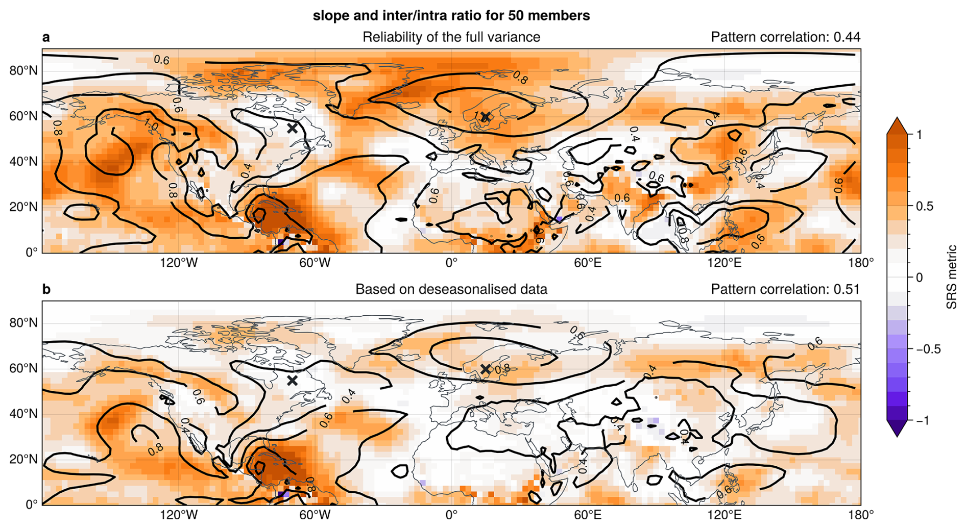
Figure 8 (shading) SRS showing the slope of z1000 spread-error curve (cf. Fig. 3) and (contours) inter-over-intra variability ratio [unitless] in the northern hemisphere for 50 member ensembles. (a) computed based on the full spread and error and (b) for de-seasonalised data, where anomalies in spread and error are computed by removing a time-dependent climatology. Crosses in both panels indicate the points in northern Europe and eastern Canada analysed in other figures. Top right title in each panel shows the area-weighted pattern correlation between the slope of spread-error curves and the inter-over-intra ratio.

5.3 Model error and under-representation of evolutions

In the previous sections we studied the effects of sampling error and natural intrinsic variability of uncertainty on the reliability of ensemble spread in subseasonal forecast models. However, forecast models may not always accurately represent all physical processes and can hence misrepresent the flow-dependence of the forecast uncertainty. In this section we assess model error effects in two complementary ways: by comparing different forecast systems and by using a perfect-model framework within a single system.

A comparison between the IFS model primarily analysed in this study and the CNRM model (Fig. S2) shows qualitatively similar large-scale spatial patterns of spread reliability and a comparable dependence on ensemble size, despite the much smaller CNRM sample. This consistency suggests that the large-scale geography of spread reliability is strongly influenced by flow-dependent variability in the underlying physical system of the atmosphere, while model-specific errors primarily modulate, rather than determine, these patterns. Nevertheless, quantitative differences between models indicate that model error may still affect the regional amplitude of reliability.

To quantify model-error effects more directly within a single forecast system, we performed an analysis using a perfect-model approach: instead of computing the errors of the prediction as difference between the ensemble mean and re-analysis data (which we regard as quasi-observations), we assumed the truth to be given by one of the ensemble members of the forecast. The prediction errors for an M member forecast are then given by the mean of the remaining M−1 ensemble members and that single selected member. The associated ensemble spread is also computed based on M−1 members. This approach ensures that the model spread is on average exactly equal to the prediction error, i.e., we have a perfectly reliable ensemble. However, this exact equality only holds if the approach is performed M times, i.e., once for each of the ensemble members of the original ensemble, and then averaged over these M sets. By only computing the perfect-model error and variance once for every given forecast (so based on a single “model truth”), we retain the same sampling as is given for the true errors computed based on re-analysis data.

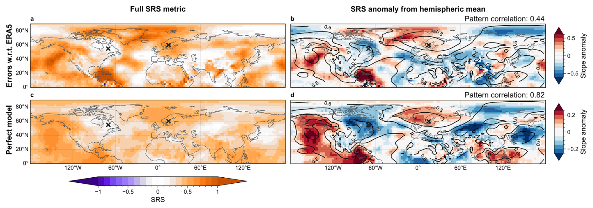
Figure 9 SRS describing the slope of z1000 spread-error curves with errors computed (a) with respect to re-analysis data and (c) based on the perfect model approach, i.e., with respect to a single ensemble member. (b) and (d) show the slope anomalies, computed as deviations from the hemispheric means, to highlight spatial structures. Contour lines in (b) and (d) show inter-over-intra ratio [unitless] with pattern correlations between slope and ratio over the northern hemisphere are indicated in the top right. All panels based on 50 member ensembles. Points in northern Europe (60° N$/$15° E) and eastern Canada (55° N$/$70° W) are indicated by crosses. Note that panels (b) and (d) use different colour scales to emphasise the similarity of spatial patterns; the smaller anomaly magnitudes in (d) are evident from the reduced colour-bar range.

Figure 9 shows the SRS in the northern hemisphere for 50-member ensembles computed from re-analysis data and using the perfect model approach, respectively. To highlight the spatial structures, Fig. 9b and d show the SRS anomaly from the hemispheric mean of each respective experiment. In general, the spatial patterns in reliability of the perfect model approach matches well with the reliability computed with respect to re-analysis. This agreement indicates that the spatial patterns seen in the SRS maps mostly result from spatial inhomogeneities in the physical system (see Sect. 5.2). The correlation between SRS and inter-over-intra ratio for the northern hemisphere in 50-member ensembles is 0.82, further supporting the interpretation that these spatial structures are largely governed by slowly evolving modes within the underlying physical system (Fig. 9d). At the same time, magnitudes of SRS anomalies are generally smaller for the perfect-model approach, indicating that model errors in representing spread variability modulate the regional amplitude of reliability.

This interpretation is reinforced by the hemispheric-mean values: the area-weighted mean SRS is 0.395 for the perfect-model framework and 0.391 when verified against re-analysis. This small difference shows that model-error effects only weakly modify the hemispheric-mean spread reliability. Taken together, these results suggest that the large-scale structure of spread reliability is primarily governed by slowly evolving large-scale modes of variability, including teleconnections, while model errors mainly redistribute reliability at regional or smaller spatial scales.

5.4 Post-processing and practical calibration of spread

One practical way to exploit our findings is to define a “corrected variance” that enforces an SRS value of one (Fig. 10). Such a correction could be constructed in various ways, with an intuitive way being the following: let $\stackrel{\mathrm{‾}}{s^{\mathrm{2}}}$ denote the climatological mean of the ensemble spread s² at a given grid point. A post-processed variance $\widehat{s^{\mathrm{2}}}$ could be obtained based on the SRS value computed from the associated spread-error curve via $\widehat{s^{\mathrm{2}}}=\stackrel{\mathrm{‾}}{s^{\mathrm{2}}}+SR{S}^{-\mathrm{1}}\left(s^{\mathrm{2}}-\stackrel{\mathrm{‾}}{s^{\mathrm{2}}}\right)$. This transformation effectively rescales deviations of the instantaneous spread from its climatological mean according to the inverse slope of the diagnosed spread–error relationship. Importantly, the climatological mean spread is not modified. The correction only adjusts the amplitude of flow-dependent spread fluctuations while preserving the underlying mean uncertainty level.

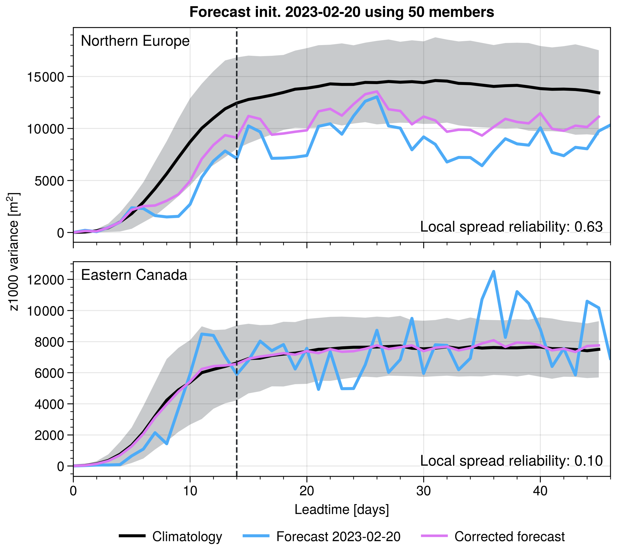
Figure 10 Evolution of z1000 ensemble variance as function leadtime at points in (a) northern Europe (60° N$/$15° E) and (b) eastern Canada (55° N$/$70° W). Black line shows climatological mean with shading indicating one standard deviation around the mean. Blue line shows variance of the example forecast initialised 20th February 2023. Pink line shows the corrected ensemble variance for that example forecast by post-processing to achieve perfect reliability.

By construction, this rescaling ensures that ensemble variance and squared error align on average. In regions where SRS≈1, the ensemble spread already provides a reliable estimate of forecast uncertainty and the correction is therefore negligible, preserving genuine flow-dependent information. In regions where SRS≪1, fluctuations in ensemble spread are not strongly linked to variations in forecast error. In such cases, the correction effectively reduces the influence of these unreliable fluctuations and shifts the variance estimate closer to its climatological baseline, leading to a more stable and statistically consistent measure of uncertainty. In areas with very small inter-variability, the corrected variance therefore remains close to the climatological mean, reflecting the limited intrinsic potential for windows of opportunity.

This adjustment can be applied in real time and provides a transparent bridge between ensemble output and user needs for calibrated risk estimates. We emphasise that the approach assumes an approximately linear and stationary spread–error relationship. More sophisticated implementations could allow the correction factor to depend on season or flow regime, although such refinements are beyond the scope of the present study.

The ideas described in this section follow closely suggestions proposed by Hopson (2014) based on ideal statistical models, where large case-to-case variability is necessary to obtain reliable and practically useful spread forecasts. The present results provide an empirical demonstration of this principle in operational subseasonal ensemble forecasts.

5.5 Effect of temporal averaging

Another practical way to improve the reliability of subseasonal uncertainty estimates that emerged from this study, in addition to a direct post-processing discussed in Sect. 5.4, is through additional time averaging. Starting from daily spread values, averaging the spread over subseasonal lead times suppresses spurious intra-forecast variability and increases the stability of the spread-error relationship, particularly when the relevant signal originates from slowly evolving large-scale modes. Such time-averaging approaches mimic the effect of a larger ensemble sizes and can enable even 10-member ensembles to outperform the daily reliability of larger ensembles based on the SRS, as shown in Fig. 11. This improvement arises because averaging reduces sampling-induced variability in the ensemble variance, analogous to increasing the effective ensemble size. Alternatively, one can first average the ensemble members in time and then compute spread and error from these weekly means, which acts as a low-pass filter and emphasises slow variability. Such weekly mean datasets are widely used at subseasonal leadtimes. Supplementary Fig. S3 compares these two strategies and supports the finding of enhanced reliability through time-averaging, with subtle regional differences: for example, over the polar Atlantic, averaging the daily spread yields higher reliability (larger SRS) than computing spread from averaged fields. This difference potentially suggests that flow-dependent reliability in this region is partly linked to faster synoptic variability rather than predominantly slow modes.

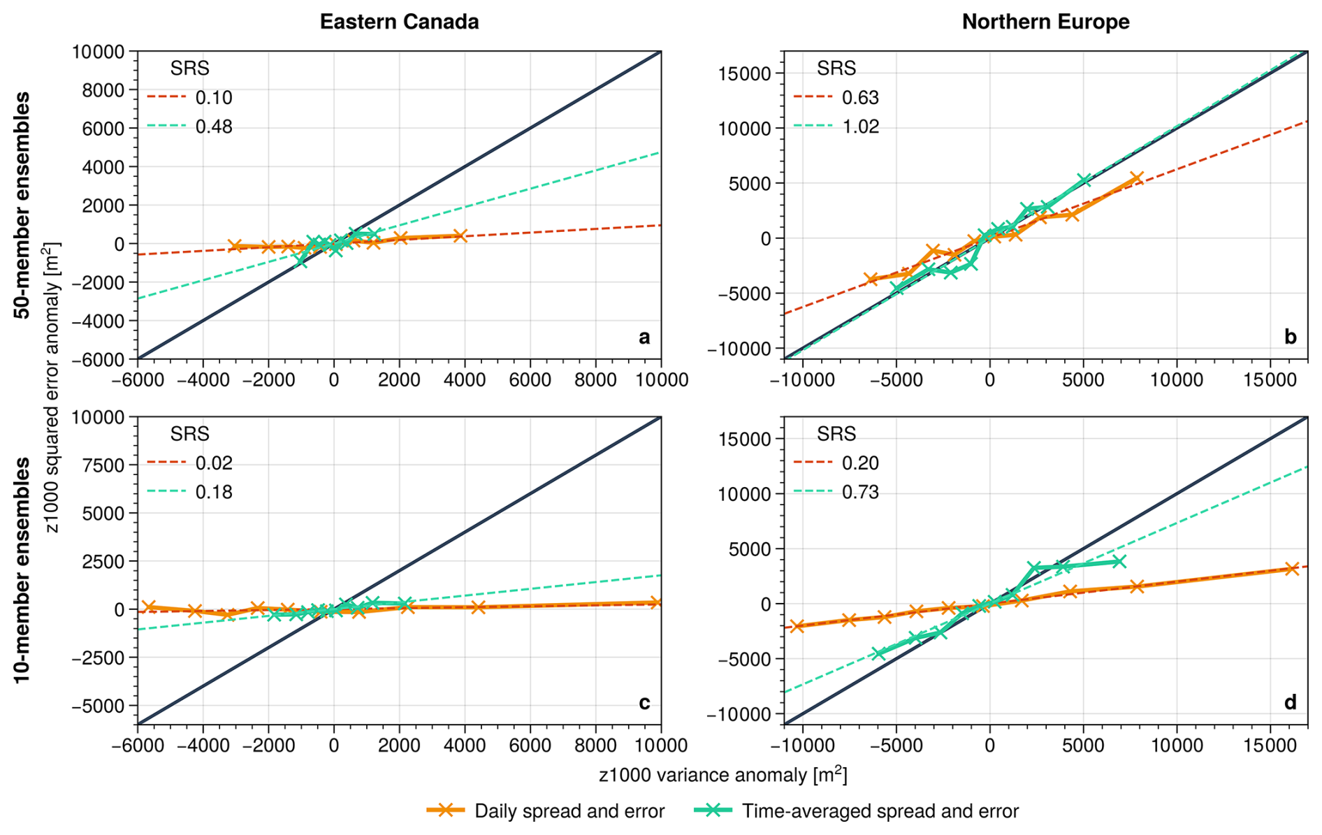
Figure 11 Comparison between reliability of daily spread values and spread averaged over subseasonal leadtimes (days 14–46) at points in (a, c) eastern Canada (55° N$/$70° W) and (b, d) northern Europe (60° N$/$15° E). Top row shows reliability in 50-member ensembles, bottom row in 10-member ensembles. Numbers in the top-left corner of each panel indicate the SRS, describing the slopes of linear fits through the reliability curve.

While time averaging can improve reliability, other factors such as systematic model biases also influence the spread-error relationship. A systematic displacement of the ensemble mean adds a constant contribution to the squared-error term, systematically shifting each point in a spread-error scatter plot (like Fig. 2b) while leaving its slope unchanged. On the other hand, ensemble mean biases can affect the ensemble spread when internal dynamics couple the mean flow to extreme behaviour. Rupp et al. (2024), for example, discuss how an anomalous position of the Atlantic storm track in the ensemble mean flow can lower the likelihood of storms over northern Europe, thereby reducing ensemble variance in that region. For our analysis framework, however, such cases can simply be considered as model errors in terms of spread itself and should be diagnosable thorough perfect model approaches as done in Sect. 5.3.

6 Conclusions and discussion

Our analysis of subseasonal winter-time forecasts, aided by an idealised toy model, shows that the reliability of ensemble spread depends on three intertwined factors: (1) sampling error (either related to a small ensemble size or to a small number of ensemble forecast), (2) the strength of the contribution of physically driven variability in intrinsic uncertainty and (3) how well the model captures this variability. Regions such as northern Europe, the mid-east Pacific and the tropical west Pacific exhibit consistently high SRS values (i.e., high spread reliability), often exceeding 0.6 for 50-member ensembles. Accordingly, our results should not be interpreted as identifying regions of uniformly high forecast skill, but rather regions where forecast uncertainty and error vary in a flow-dependent manner that is reliably captured by ensemble spread. These SRS hotspots coincide with areas influenced by slowly varying atmospheric modes that provide “windows of forecast opportunity”. In northern Europe, for instance, the downward influence of the polar stratosphere has been linked to multi-week periods of anomalously low spread, due to a reduction in storm-induced synoptic variability (Spaeth et al., 2024a; Rupp et al., 2024). This process seems to be well-captured in forecast models and hence leads to high values of SRS in northern Europe. The mid-east Pacific signal could reflect ENSO modulation of the jet, while tropical West Pacific reliability may arise from the MJO’s planetary wave response, though these connections remain speculative and warrant targeted process studies.

In contrast, eastern Canada displays almost no reliability even when 100 members are available, with SRS essentially zero. Consistently, the ensemble variance in eastern Canada is nearly constant through the subseasonal range, suggesting the atmosphere itself offers little low-frequency modulation of forecast uncertainty. Enlarging the ensemble further would therefore add computational cost without creating useful information in terms of forecast uncertainty because the intrinsic potential for windows of opportunity is vanishingly small.

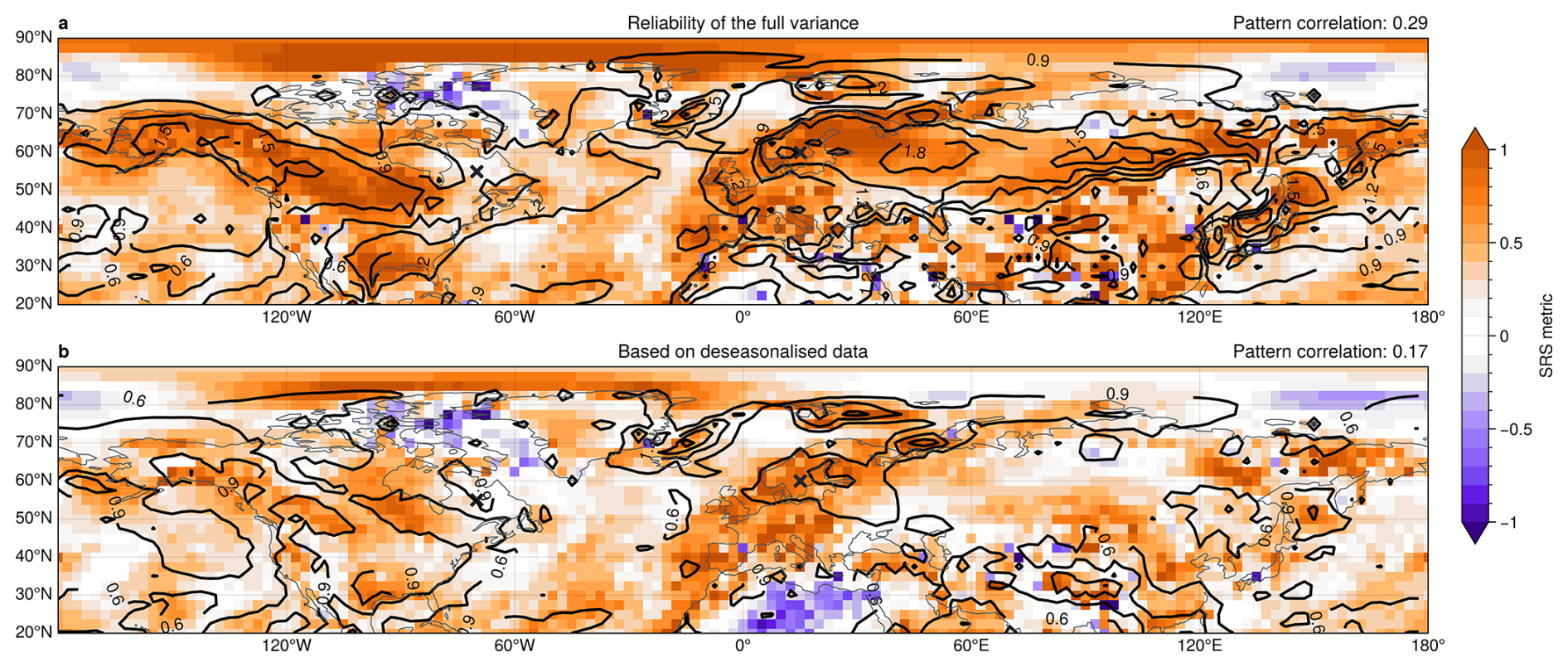
Figure 12 As Fig. 8 but for t2m rather than z1000.

Beyond the contrast between highly reliable regions such as northern Europe and nearly constant-spread regions such as eastern Canada, the North Atlantic sector itself exhibits additional structure (cf. Fig. 3). In particular, the higher reliability over the northern part of the basin compared to the southern centre of action suggests that mechanisms projecting onto the NAO may influence forecast uncertainty asymmetrically. This behaviour is consistent with the pronounced maximum in relative spread variability over the northern North Atlantic (Fig. 1). While enhanced variability is also present in the subtropical North Atlantic, it appears displaced further south (around 20–30° N), suggesting that distinct processes may contribute there. Previous work has shown that subseasonal spread anomalies linked to stratospheric variability can project more strongly onto northern NAO regions than onto the southern centre (Spaeth et al., 2024a). In addition, modulation of synoptic eddy activity has been identified as a key mechanism shaping subseasonal forecast spread over the North Atlantic (Rupp et al., 2024), suggesting that variability in eddy magnitude, rather than purely meridional shifts of storm tracks, may contribute to this asymmetric reliability pattern. Given the limited number of forecast initialisations, however, finer-scale spatial details should be interpreted with caution.

Generally, the reliability of spread forecasts can vary for different variables analysed. This dependence partly arises through different flow dependences of the ensemble spread on the basic state (as, e.g., shown in Spaeth et al., 2024b). Figure 12a shows the SRS metric for the 2-metre temperature (t2m) and compares it to the t2m inter-variability. Two pronounced regions of high SRS are clearly visible around 60° N, forming band-like structures across the two major northern-hemispheric landmasses. These regions also show high values of inter-over-intra variability, further suggesting that subseasonal reliability is mostly driven by slowly evolving modes, although the overall pattern correlation for the northern hemisphere is relatively small. Further, we find that the high SRS for the t2m field in these regions mostly arises from the seasonal winter-to-spring transition in surface temperatures, which is most pronounced in the mid-latitudes and over land. Correspondingly, the SRS strongly decreases in those regions when computing the reliability based on deseasonalised spread data (Fig. 12b).

The results presented here might also be relevant with regard to the so-called “signal-to-noise paradox” (SNP), described by Scaife and Smith (2018). The paradox refers to an apparent mismatch in climate and seasonal forecasting systems, in which forecasts correlate better with observed variability than with their own ensemble members. According to Scaife and Smith (2018), such a situation arises if the unpredictable component (noise) of the observed atmosphere is systematically smaller than the ensemble spread suggests, leading to forecasts being paradoxically under-confident.

Recent work by Roberts and Vitart (2024) investigates ensemble reliability and SNP in large-ensemble subseasonal forecasts, with particular emphasis on the role of ensemble size and sampling effects in diagnosing apparent under-confidence. Specifically, they demonstrate how reliability diagnostics and SNP metrics depend sensitively on ensemble size and highlights the role of large ensembles in reducing sampling artefacts when interpreting apparent under-confidence. While their focus is primarily on the amplitude of predictable signal relative to climatological ensemble spread and the overall reliability characteristics of the forecast system, rather than on flow-dependent variability of spread fluctuations, studies like Scaife and Smith (2018) or Roberts and Vitart (2024) underline the importance of carefully interpreting reliability measures in the subseasonal-to-seasonal regime. Similarly, Strommen et al. (2023) suggest that the occurrence of SNP is equivalent to reliability diagrams exhibiting slopes greater than unity, although their reliability metric differs from our spread-error slopes. Despite methodological differences, both the SNP framework and our spread-error analysis highlight the fundamental importance of accurately capturing atmospheric variability and ensemble spread characteristics in order to interpret forecast confidence in a dynamically consistent manner.

While our framework does not directly quantify the absolute level of ensemble spread (which is central to the SNP), it does address whether fluctuations in spread (e.g., departures from climatology) reliably represent variations in atmospheric uncertainty. Regions identified in our study as having low inter-over-intra variability ratios also exhibit correspondingly poor spread reliability and low SRS. Such conditions might indirectly reflect scenarios favourable for the paradox, potentially arising from systematic misrepresentations of ensemble spread variability. Indeed, Karpechko et al. (2025) demonstrate that teleconnections influencing the subseasonal skill are also associated with changes in the ensemble spread, further supporting a potential linkage between slowly varying atmospheric modes, ensemble spread representation, and the SNP. A more direct analysis of how precisely variability in spread connects to the paradox remains an open question and future research explicitly bridging these concepts could help clarify their relationship.

Although the present manuscript emphasises low-spread situations in the context of windows of opportunity, the SRS metric itself is symmetric with respect to the spread distribution and therefore reflects the reliability of spread fluctuations at both the low- and high-spread ends of the spectrum. Low-spread regimes (i.e. windows of opportunity) are dynamically as relevant as high-spread regimes, i.e., walls of adversity. High-spread states correspond to periods of enhanced intrinsic uncertainty and reduced predictability. For example, episodes of strong stratosphere-troposphere coupling during intense upward wave activity can lead to uncertainty in the evolution of the polar vortex, including whether it undergoes a sudden stratospheric warming or re-strengthening. If such uncertainty propagates downward, it may temporarily amplify tropospheric ensemble spread, representing a dynamically driven high-uncertainty regime. From a dynamical perspective, both ends of the spectrum arise from flow-dependent modulation of intrinsic forecast uncertainty by slowly evolving large-scale modes; the difference lies only in whether those modes temporarily suppress or amplify error growth.

In summary, the ability of an ensemble to convey reliable uncertainty forecasts depends on two questions: does the physical system provide a window of opportunity, and is the model accurate enough to detect it? Our spread-error framework shows that, over large areas of the Northern Hemisphere, slowly varying teleconnections modulate intrinsic forecast uncertainty, thereby creating the potential for flow-dependent reductions in intrinsic forecast uncertainty (windows of opportunity) that can be reliably detected with 50 to 100 members. On the other hand, regions lacking a strong influence of such slow modes remain unreliable in terms of spread-error relationship even when the ensemble size is large. While low-spread situations and associated improved forecast uncertainty may enable enhanced forecast skill, the existence of a potential for windows of opportunity does not by itself guarantee skillful forecasts, which depend on additional aspects of model performance and predictability.