Impacts of tropical forecast errors on two extreme precipitation events: insights from relaxation experiments using machine-learning weather prediction models

This study explores the use of relaxation experiments in 2 machine learning-based weather prediction (MLWP) models to identify sources of subseasonal predictability in comparison to a traditional numerical weather prediction (NWP) system. Tropical relaxation involves nudging specific tropical regions of a model toward reanalysis data to isolate their influence on forecast skill. We apply this technique to Pangu-Weather (fully data-driven) and NeuralGCM (hybrid) and compare the experiments to the Unified Forecast System (UFS). The focus is on the week 3–4 forecast of 2 major precipitation events in western North America in winter 2022/2023, both linked to Madden–Julian Oscillation (MJO) activity. For the 2 cases, MLWP models exhibit higher forecast skill than the UFS at subseasonal lead times. Though tropical relaxation improves the skill in all forecast systems, gains are greater for UFS, reflecting the MLWP models' stronger baseline performance. A Rossby wave source (RWS) analysis shows that tropical relaxation consistently improves the large-scale dynamic processes associated with the tropical–extratropical teleconnections leading to both events. These results highlight the potential of relaxation experiments as an effective diagnostic for understanding and improving subseasonal forecasts, especially in emerging MLWP systems.

1 Introduction

Subseasonal-to-seasonal (S2S) forecasts targeting lead times of 2 weeks to 2 months are critical for anticipating extreme weather events, supporting agriculture, and enhancing community resilience (White et al., 2022). Despite steady advances in numerical weather prediction (NWP), reliable predictions beyond 2 weeks remain limited by intrinsic predictability constraints and systematic model biases (Vitart et al., 2012). Leveraging known sources of subseasonal predictability, including those originating at low latitudes such as the Madden–Julian Oscillation (MJO; Madden and Julian, 1972), is essential for improving forecast skill (Cassou, 2008; Lin et al., 2009; Merryfield et al., 2020). As machine learning-based weather prediction (MLWP) progressively emerges as a powerful tool for predictions, this study aims to investigate tropical sources of subseasonal predictability in MLWP systems.

The growing number of studies demonstrating skillful medium-range MLWP forecasts suggests that these systems also offer a promising path for advancing S2S forecasting (Weyn et al., 2021; Chen et al., 2024), even as several important challenges remain. For instance, data-driven models like Pangu-Weather (Bi et al., 2022) and hybrid approaches such as NeuralGCM (Kochkov et al., 2024) have demonstrated skill comparable to state-of-the-art NWP models in the medium range. However, MLWP models can be highly sensitive to initial condition perturbations (Vonich and Hakim, 2024; Tian et al., 2024), raising questions about their robustness for longer lead times. Though MLWP performance on subseasonal timescales including their sensitivity to teleconnection patterns remain less well understood, recent results highlight their potential also for this time-scale (e.g. Diao and Barnes, 2025). Moreover, their relatively low computational costs enable systematic studies of potential sources of predictability.

A common diagnostic for assessing sources of predictability in NWP models is the relaxation technique, which nudges forecasts toward a reference dataset over specific regions (Jung et al., 2010; Magnusson, 2017). This method has successfully illuminated the role of tropical forecast errors in extratropical forecast skill and the potential to improve the representation of MJO-related teleconnections (Dias et al., 2021; Vitart and Balmaseda, 2024). Though such experiments can be computationally demanding, they provide valuable insight into error propagation and regional influence on forecast skill. The application of relaxation techniques to MLWP models has not been widely tested. Evaluating whether tropical relaxation improves mid-latitude subseasonal forecasts in MLWP models could inform both efforts related to their physical consistency and future model development (Perkan and Zaplotnik, 2025). Here, we investigate relaxation in MLWP forecasts for 2 high-impact precipitation events in western North America during winter 2022–2023 that were influenced by MJO activity and La Niña conditions. These events occurred from late December to mid January and late February to early March, respectively, and involved contrasting large-scale circulation patterns. We compare the prediction skill of ensemble forecasts from Pangu-Weather, NeuralGCM, and an experimental version of the Unified Forecast System (UFS) under different relaxation configurations, complementing analyses by Moore et al. (2026).

The primary objectives of this study are threefold. First, we test the general feasibility of applying the relaxation technique to both a fully MLWP-based and a hybrid weather prediction model. Second, we evaluate the impact of relaxation in these models in comparison to an NWP model, specifically in the context of subseasonal forecasts. Finally, we assess whether correcting tropical forecast errors through relaxation leads to improved mid-latitude forecast skill in the 2 models. The data, models, nudging technique and Rossby wave source diagnostic are introduced in Sect. 2. Results are presented in Sect. 3. The study ends with a concluding discussion in Sect. 4.

2 Data and methodology

2.1 Ensemble design and initialization approach

Pangu-Weather, NeuralGCM, and UFS forecasts are all initialized from the same ensemble of data assimilations (EDA) from the ERA5 reanalysis data set (Hersbach et al., 2020). The EDA includes 10 ensemble members that account for uncertainties in the observations and the underlying model by perturbing model physical tendencies in the short forecasts that link subsequent analysis windows. It contains all atmospheric variables to initialize the models of this study and is available on a regular latitude–longitude grid with 0.5° × 0.5° grid spacing. The EDA data is regridded with bilinear interpolation to match each model's grid spacing.

The subseasonal forecasts for the 2 cases are initialized on 15 December 2022 and 2 February 2023, respectively. The initialization of the subseasonal forecasts is achieved through a time-lagged combination of ensemble members from EDA following the approach of Moore et al. (2026). For example, the forecast initialized on 15 December 2022, 00:00 UTC incorporates ensemble members from forecasts issued on 14 December 2022, 12:00 UTC, 15 December 2022, 00:00 UTC and 15 December 2022, 12:00 UTC. With 10 ensemble members at each time, this yields a 30 member time-lagged ensemble. This methodology is applied consistently for the February case study.

2.2 MLWP and NWP forecast models

This study evaluates subseasonal prediction skill using 3 distinct modeling approaches: (1) an experimental version of the National Oceanic and Atmospheric Administration (NOAA) UFS, a state-of-the-art NWP model (Jacobs, 2021), (2) NeuralGCM, a hybrid neural network-based general circulation model (Kochkov et al., 2024), and (3) Pangu-Weather, a purely data-driven MLWP model (Bi et al., 2022).

2.2.1 UFS

The UFS is the Earth system modeling framework for current operational NOAA prediction systems, including the Global Forecast System (GFS) and Global Ensemble Forecast System. Experiments were performed with a prototype UFS version (labeled “HR1”). This coupled ocean–atmosphere–ice–wave prediction system employs the Finite-Volume Cubed-Sphere Dynamical Core (Zhou et al., 2019) and was run globally at C96 resolution (approximately 1° latitude/longitude) with 6 h forecast outputs. The HR1 prototype includes updated GFDL microphysics and other physics packages, and its performance has been shown to be comparable to the operational GFS for large-scale forecasts while improving the representation of precipitation and mesoscale processes. In this study, the UFS model is used as a benchmark to compare the prediction skill of Pangu-Weather and NeuralGCM for the 2 cases.

2.2.2 NeuralGCM

NeuralGCM is a hybrid machine learning-enhanced general circulation model (Kochkov et al., 2024). The model leverages a differentiable dynamical core for solving the discretized governing dynamical equations as in NWP models and an ML-based physics module that parameterizes per vertical column the effect of unresolved physical processes with a neural network. In this study, subseasonal forecasts and relaxation experiments utilize the 1.4° resolution auto-agressive model, which provides output on 37 vertical sigma levels. On seasonal to climate timescales, the NeuralGCM models exhibit robust and stable performance when integrating the 1.4° deterministic configuration for periods of up to approximately 2 years (Kochkov et al., 2024). The deterministic model setting is used such that ensemble members only diverge because of different initial conditions taken from the EDA of ERA5. Sea surface temperature (SST) and sea ice concentration are prescribed daily from ERA5. The use of prescribed SST compared to a coupled system as in UFS reduces 1 source of forecast uncertainty. To assess the potential advantage of NeuralGCM over UFS, we conduct additional experiments with NeuralGCM using fixed SST taken at initialization time from ERA5 (Fig. A1). We find that the difference between runs with fixed and prescribed SST does not explain the different skill between NeuralGCM and UFS for these 2 events (see Sect. 3). Accordingly, all results with NeuralGCM shown in this study are based on experiments with prescribed SST.

2.2.3 Pangu-Weather

Unlike UFS and NeuralGCM, which integrate a full GCM dynamical core and numerically solve the governing equations of atmospheric motion, Pangu-Weather is a fully data-driven deep learning model trained on 39 years (1979–2017) of ERA5 reanalysis data (Bi et al., 2022). Pangu-Weather operates at a regular latitude–longitude grid of 0.25° with 13 pressure levels. As Pangu-Weather is only based on atmospheric fields, SST and sea ice concentration are not accounted for. It is trained separately for 1, 3, 6, 24 h lead times. Longer lead times can be reached through autoregressive inference. Avoiding explicit time-stepping of the primitive equations, reduces computational cost substantially. In this study, we only use the Pangu-Weather model with a 24 h time step for generating subseasonal forecasts and relaxation experiments. Pangu-Weather ensemble members are generated using perturbations from the EDA described in Sect. 2.1.

2.3 Verification and climatology data

All forecasts are relaxed and evaluated against ERA5 reanalysis data (Hersbach et al., 2020). This dataset provides analyses of atmospheric conditions at 0.25° grid spacing (Hersbach et al., 2020). ERA5 data are remapped using bilinear interpolation to each model's native resolution. Daily climatological means from the ERA5 for 1990–2019 were used to compute anomalies of all atmospheric variables. A sliding window is applied around each day-of-year and time-of-day combination, with weights that decrease linearly from the center to zero. This approach smooths the climatology by reducing sample noise, though it slightly diminishes the seasonal amplitude. These climatological means, obtained from the WeatherBench2 dataset, are calculated following the method of Rasp et al. (2020). All models generate 30 d ensemble forecast using the method mentioned in the Sect. 2. For each case, we examine the subseasonal prediction of the large-scale circulation over the North Pacific and western North America at 3–4 weeks lead time. Forecasts are averaged daily during the validation periods ranging from 30 December 2022–13 January 2023 and 17 February–3 March 2023, respectively.

2.4 Setup of relaxation experiments

2.4.1 Setup in MLWP models

Relaxation, also referred to as nudging, is an established method in NWP models and has been used in many contexts including the assessment of the role of specific regions for subseasonal predictability (Jung et al., 2010). This approach normally incorporates an additional term into the NWP model's prognostic equations to steer the model state toward reference data thereby constraining the model's evolution within the relaxation domain (Jung et al., 2010; Magnusson, 2017). In this study, we apply the relaxation to the three-dimensional model state vector x_t at leadtime t in NWP and MLWP models using the following equation

$$\begin{array}{}\text{(1)}& {\widehat{\mathit{x}}}_t={\mathit{x}}_t+\mathit{\lambda }({\mathit{x}}_{\text{ref},t}-{\mathit{x}}_t),\end{array}$$

where x_ref,t is the reference data (ERA5 reanalysis) and λ is the relaxation coefficient that determines the strength of the relaxation. After applying the relaxation function, we provide the corrected state vector ${\widehat{\mathit{x}}}_t$ to the model and continue the forecast to the next lead time.

To prevent discontinuities at the boundaries of the relaxed region, we apply a hyperbolic tangent function similar to Magnusson (2017) to create a tapering region (Fig. A2). This function modulates the relaxation coefficient λ near the edges, ensuring a gradual change from the nudged to the free-running model areas. The transition function can be formulated as

$$\begin{array}{}\text{(2)}& \mathit{\lambda }\left(\mathit{\varphi }\right)={\mathit{\lambda }}_{\mathrm{0}}\left[\mathrm{0.5}-\mathrm{0.5}\tanh \left({\displaystyle \frac{\mathit{\varphi }-a}{b}}\right)\right],\end{array}$$

where λ₀ is the maximum relaxation coefficient. We take λ₀=1.0, which means that each forecast in the relaxed region is corrected by 100 % at each time step. Parallel experiments with λ₀=0.33 (Magnusson, 2017) yield qualitatively similar results (not shown). ϕ denotes the latitude, a is the central point of the transition, and b controls the latitudinal width of the tapering region. This formulation ensures a gradual transition of λ(ϕ) from λ₀ to 0 at the boundaries.

Table 1 Description of experimental setups and their abbreviations.

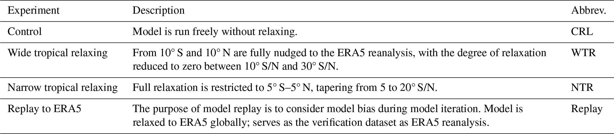
Table 2 Variables used for relaxation in UFS, NeuralGCM, and Pangu models. In addition, the UFS model applies relaxation to pressure, which is not available in MLWP models.

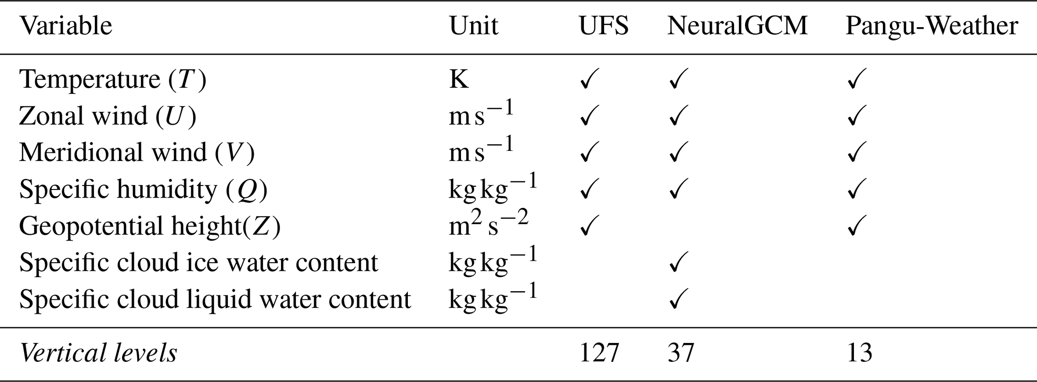
Note: “✓” indicates the variable is used for relaxation in the given model.

The sensitivity to the width of the transition is tested in this study by conducting 3 types of relaxation experiments. These are Control (CRL), narrow tropical relaxation (NTR, relaxing from 20° S to 20° N including the tapering region) and wide tropical relaxation (WTR, relaxing from 30° S to 30° N including the tapering region). WTR is designed to assess the overall impact of the entire tropics, whereas NTR focuses more strictly on the deep tropics. An additional experiment is a replay experiment during which relaxation is applied globally (Replay). The Replay experiment allows to assess the effect of potential model biases and serves as a verification dataset when calculating the anomaly correlation coefficient (ACC; Wilks, 2011) and mean absolute error (MAE) in the later analysis. More detailed information are available in Table 1 and MLWP model replays are in the supplementary Fig. A3.

In UFS, horizontal wind components, geopotential, specific humidity, and temperature are nudged (Table 2). To ensure a consistent comparison across models, we relax variables that are common among the model configurations whenever possible and follow the UFS nudging configuration as a reference. However, the prognostic variable sets differ between the MLWP models. For example, NeuralGCM includes cloud liquid and ice water content that are not available in Pangu-Weather. As a result, the set of relaxed variables cannot be made identical across all models.

In Pangu-Weather, variables at all 13 pressure levels are nudged during model integration, while surface variables (e.g., 2 m temperature) are excluded from relaxation. In NeuralGCM, variables between the lower troposphere and the tropopause are relaxed, including cloud ice and liquid water content. Sensitivity tests indicate that relaxing geopotential in NeuralGCM introduces large negative forecast errors, likely due to its strong dynamical coupling with the model state. Therefore, geopotential relaxation is not applied in NeuralGCM. The relaxation is applied every 24 h in both MLWP models.

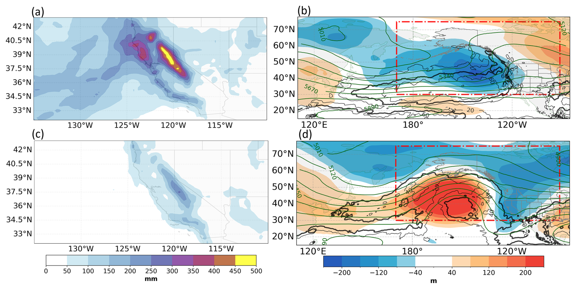
Figure 1 ERA5-based accumulated precipitation (shading in mm) 3–4 weeks after forecast initialization for (a) case study 1 and (c) case study 2 (30 December–13 January for case 1, and 17 February–3 March for case 2). Mean 500 hPa geopotential height anomaly relative to 1990–2019 daily climatology (shading in m), 500 hPa geopotential height (green solid lines in m), and 850 hPa water vapour flux (black contours in $\mathrm{g}{\mathrm{kg}}^{-\mathrm{1}}\mathrm{m}{\mathrm{s}}^{-\mathrm{1}}$; 40 and 20$\mathrm{g}{\mathrm{kg}}^{-\mathrm{1}}\mathrm{m}{\mathrm{s}}^{-\mathrm{1}}$ is highlighted in b and d separately) 3–4 weeks after initialization for (b) case study 1 and (d) case study 2. Red rectangle marks the area for calculating latitude-weighted centered ACCs and MAEs.

Forecasts are evaluated in terms of atmospheric quantities that describe the large-scale flow favouring the 2 precipitation events. Precipitation itself is not analysed as the MLWP models used here do not directly predict precipitation. Instead, we analyse the representation of horizontal water vapour transport which has been linked to heavy precipitation events (e.g., Lavers et al., 2017). Here, the horizontal water vapour transport is computed as the product of specific humidity and horizontal wind components at 850 hPa (F=qV). The magnitude of this vector quantity is shown in the figures. It should still be noted that moisture transport represents only the dynamical supply of water vapour and does not directly account for microphysical processes that control precipitation formation, which constitutes a limitation of this diagnostic.

2.4.2 Setup in UFS

Relaxation experiments in UFS follow the approach of Dias et al. (2021). An Incremental Analysis Update (IAU) is used to reduce shocks by nudging the model toward ERA5 reanalysis. Increments are calculated as differences between 3 h forecasts and reanalysis data, then applied over a 6 h forecast window in a repeated “replay” cycle. In the UFS experiments, the λ₀ relaxation coefficient of 1 is used in the specified latitude bands for WTR and NTR experiments.

2.4.3 Rossbywave source analysis

Following Sardeshmukh and Hoskins (1988), the Rossby wave source (RWS) represents the vorticity tendency through divergent outflow in the upper troposphere, primarily driven by tropical convection. The full RWS is defined as the negative divergence of the product of the divergent wind vector and the absolute vorticity, i.e.,

$$\begin{array}{}\text{(3)}& \mathrm{RWS}=-\mathrm{\nabla }\cdot \left({\mathbf{V}}_{\mathit{\chi }}\mathit{\zeta }\right),\end{array}$$

where ${\mathbf{V}}_{\mathit{\chi }}=(u_{\mathit{\chi }},v_{\mathit{\chi }})$ is the divergent wind and ζ is the absolute vorticity. Expanding Eq. (3) gives

$$\begin{array}{}\text{(4)}& \mathrm{RWS}=-\left(u_{\mathit{\chi }}{\displaystyle \frac{\partial \mathit{\zeta }}{\partial x}}+v_{\mathit{\chi }}{\displaystyle \frac{\partial \mathit{\zeta }}{\partial y}}+\mathit{\zeta }\mathrm{\nabla }\cdot {\mathbf{V}}_{\mathit{\chi }}\right).\end{array}$$

This diagnostic has been widely used to identify tropical sources of Rossby waves and their downstream propagation patterns (e.g., Hoskins and Karoly, 1996; Seo and Son, 2016; Moore et al., 2026).

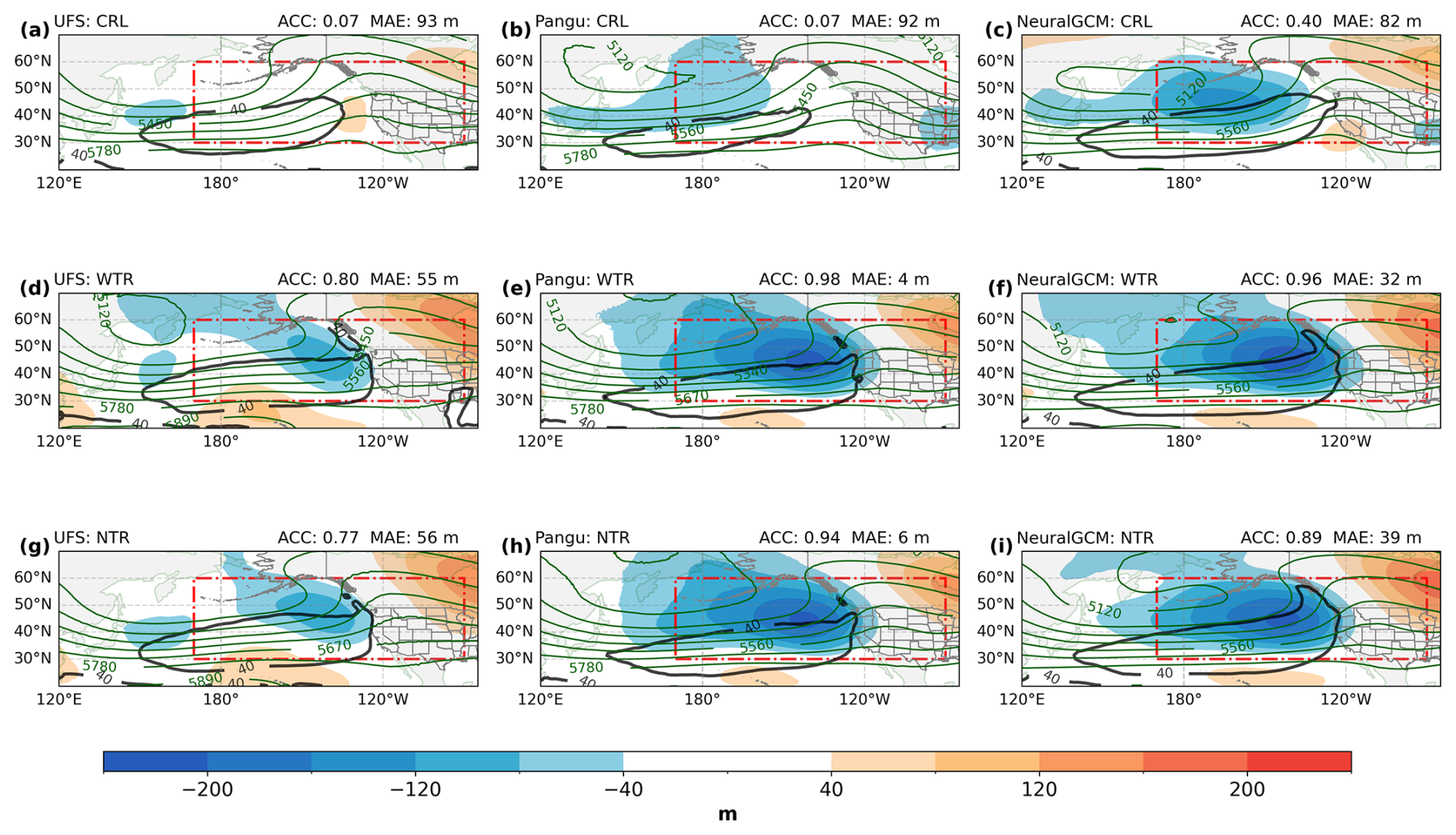
Figure 2 Week 3–4 ensemble mean of forecasts initialized on 15 December 2022 showing 500 hPa geopotential height anomaly relative to daily climatology (shading in m), 500 hPa geopotential height (green contours in m), and 850 hPa moisture transport (black solid line at magnitude of 40 $\mathrm{g}{\mathrm{kg}}^{-\mathrm{1}}\mathrm{m}{\mathrm{s}}^{-\mathrm{1}}$ is in bold). The columns show forecasts by (a, d, g) UFS, (b, e, h) Pangu-Weather and (c, f, i) NeuralGCM. The rows show experiments (a–c) CRL (d–f) WTR and (g–i) NTR. Red rectangle denotes the area for calculating the latitude-weighted ACC and MAE from the ensemble mean.

3 Tropical relaxation experiment results: 2 case studies

The 2 precipitation events considered in this study occurred outside the training period of both MLWP models. Building on the findings of Moore et al. (2026), we evaluate the MLWP forecast skill using the latitude-weighted centered ACC and the MAE of 500 hPa geopotential height over the eastern North Pacific and western North America (30–60° N, 170° E–90° W). The ACC can be interpreted as the pattern correlation between the verification anomaly in Fig. 1 and forecast anomalies shown in Figs. 2 and 5 in this region.

3.1 Case study 1: December 2022 to January 2023

For the first event, lasting from 26 December 2022 to mid-January 2023, the total rainfall accumulation of ERA5 exceeds 450 mm in California (Fig. 1a). In some regions, the observed accumulated precipitation even reached values up to 1000 mm (DeFlorio et al., 2024). This extreme precipitation event led to at least 21 fatalities and caused property damage estimated between USD 5–7 billion (Schubert et al., 2024). Additionally, operational forecasts from both NOAA and ECMWF exhibited relatively large forecast errors during this event (Moore et al., 2026).

The synoptic situation during this 2-week period was characterized by a Rossby wave pattern featuring a positive geopotential height anomaly over the subtropical North Pacific, a negative height anomaly over the eastern North Pacific and a positive height anomaly over eastern North America. The anomalous, quasi-stationary upper-level trough over the northeastern Pacific (Fig. 1b) created a prolonged southwesterly flow along the US West Coast. It was associated with enhanced cyclone and atmospheric river (AR) activity that impacted an area extending from California to British Columbia (not shown). During the 2-week period, the mean water vapour flux (Sect. 2.4) at 850 hPa reached values of 40 $\mathrm{g}{\mathrm{kg}}^{-\mathrm{1}}\mathrm{m}{\mathrm{s}}^{-\mathrm{1}}$ at the coastline (black contours in Fig. 1b) favouring the enormous rainfall amounts in California and Oregon. From 21 to 28 December 2022, the MJO progressed through phases 4–5 in the real-time multivariate MJO (RMM; Wheeler and Hendon, 2004) phase space. This earlier MJO activity may have influenced the midlatitude circulation pattern linked to the precipitation event. The 2-week period of the event itself co-occurred with an active MJO phase 6–7 from 29 December 2022 to 9 January 2023. Though MJO phases 6–7 are on average followed by a positive geopotential height anomaly over western North America, this event featured a negative geopotential height anomaly illustrating the enormous variability in the extratropical response to the MJO as also documented by Quinting et al. (2024). Recent studies suggest that the Rossby wave pattern was enhanced by the active MJO with convection over the western Pacific, promoting the ridge-trough-ridge tripole extending from the subtropical North Pacific to eastern North America (DeFlorio et al., 2024; Moore et al., 2026).

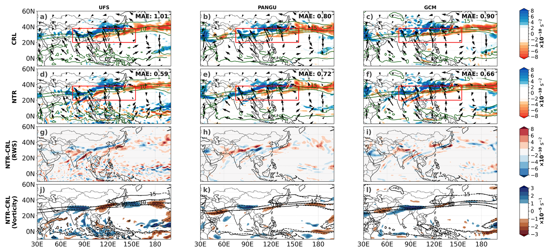
Figure 3 Comparison of ensemble-mean forecasts from CRL (a–c) and NTR (d–f) averaged for 23–30 December 2022 for UFS (a, d), Pangu-Weather (b, e), NeuralGCM (c, f). The 200 hPa RWS (10⁻¹⁰ s⁻², shading), 200 hPa ζ (green contours every 5 × 10⁻⁵ s⁻¹), 200 hPa divergent wind (arrows, m s⁻¹); RWS difference in shading between NTR and CRL in (g–i) for each model. NTR − CTL differences (j–i) in the 200 hPa ζ (10⁻⁵ s⁻¹, shading) overlaid by ζ (contours every 5 × 10⁻⁵ s⁻¹) for NTR (solid) and CRL (dashed) for UFS, Pangu-Weather and NeuralGCM.

Forecasts initialized on 15 December 2022 and valid during weeks 3–4 (30 December–13 January) are shown in Fig. 2. The CRL experiments across all models fail to adequately capture the dipole pattern of negative and positive geopotential height anomalies extending from the northern Pacific to eastern North America (Fig. 2a–c). Notably, the UFS model exhibits the lowest prediction skill for 500 hPa geopotential height, with a regional mean ACC of 0.07 and the highest MAE of 93 m (Fig. 2a). Pangu-Weather shows a similar prediction skill with an ACC of 0.07 and MAE of 92 m in the target region (Fig. 2b). The low forecast skill from CRL in Pangu-Weather might be associated with a systematic negative temperature bias (Ben Bouallègue et al., 2024), likely stemming from limitations in its model architecture and training procedure (Ennis et al., 2025). In contrast, NeuralGCM demonstrates a comparative better representation of the large-scale circulation (Fig. 2c). The 500 hPa trough extends further east and a weak positive geopotential height anomaly exists over eastern North America. This contributes to a higher subseasonal forecast skill for this case – not only in terms of geopotential height, but also regarding the representation of 850 hPa water vapour flux.

The WTR (Fig. 2d–f) and NTR (Fig. 2g–i) experiments show marked improvements in reproducing the anomalous 500 hPa geopotential height pattern over the Pacific in all 3 models. All models better represent the positive geopotential height anomaly over the subtropical North Pacific. Pangu-Weather and NeuralGCM improve the representation of the deep trough over the eastern North Pacific leading to higher ACC values. The presence of this trough is the key distinguishing feature compared to CRL in all 3 models.

The associated enhanced westerly flow leads to a band of strong 850 hPa water vapour flux exceeding 40 $\mathrm{g}{\mathrm{kg}}^{-\mathrm{1}}\mathrm{m}{\mathrm{s}}^{-\mathrm{1}}$ (the magnitude highlighted by the bold black solid line in Fig. 2). This moisture transport extends closer to the west coast of North America in the WTR and NTR experiments compared to the CRL configuration. Its proximity to the coast also better matches the verification data (Fig. 1b), indicating an improved representation of the precipitation event.

The similarity between the WTR and NTR forecasts for all models suggests that a better representation of the tropics would have improved the subseasonal forecast skill for this event. Peings et al. (2026) came to a similar conclusion based on forecast experiments with altered initial conditions in the tropics using a fully data-driven MLWP model. Note that Peings et al. examined impacts of the tropics for experiments initialized later, on 26 December, and thus focused on shorter forecast lead times.

To further understand how the relaxation in the tropics impacts the extratropical Rossby wave forcing, we analyze the RWS (Sect. 2.4.3) at 200 hPa averaged from 23–30 December 2022 (during week 2; Fig. 3), which is 1 week earlier than the validation period (week 3–4). The focus here is to analyze the establishment of the large-scale flow pattern associated with this extreme precipitation in December in the forecast. Noting that MAEs of RWS are calculated between forecasts and ERA5 in the red box (20–38° N, 75–155°E) ranging from the Maritime Continent to the western Pacific.

UFS CRL predictions consistently overestimate the divergent outflow and the resulting negative vorticity advection to the north of the MJO-related convection over the Maritime Continent and western Pacific, in the days preceding the precipitation events (Moore et al., 2026). Here, results are only shown for the NTR experiments because WTR experiments are qualitatively similar. In NTR and CRL, all models represent the band of negative RWS values over eastern Asia and an area of positive RWS over the western Pacific (Fig. 3a–f). This indicates that the 2 MLWP models of this study are physically consistent with the UFS model in representing tropical–extratropical teleconnections.

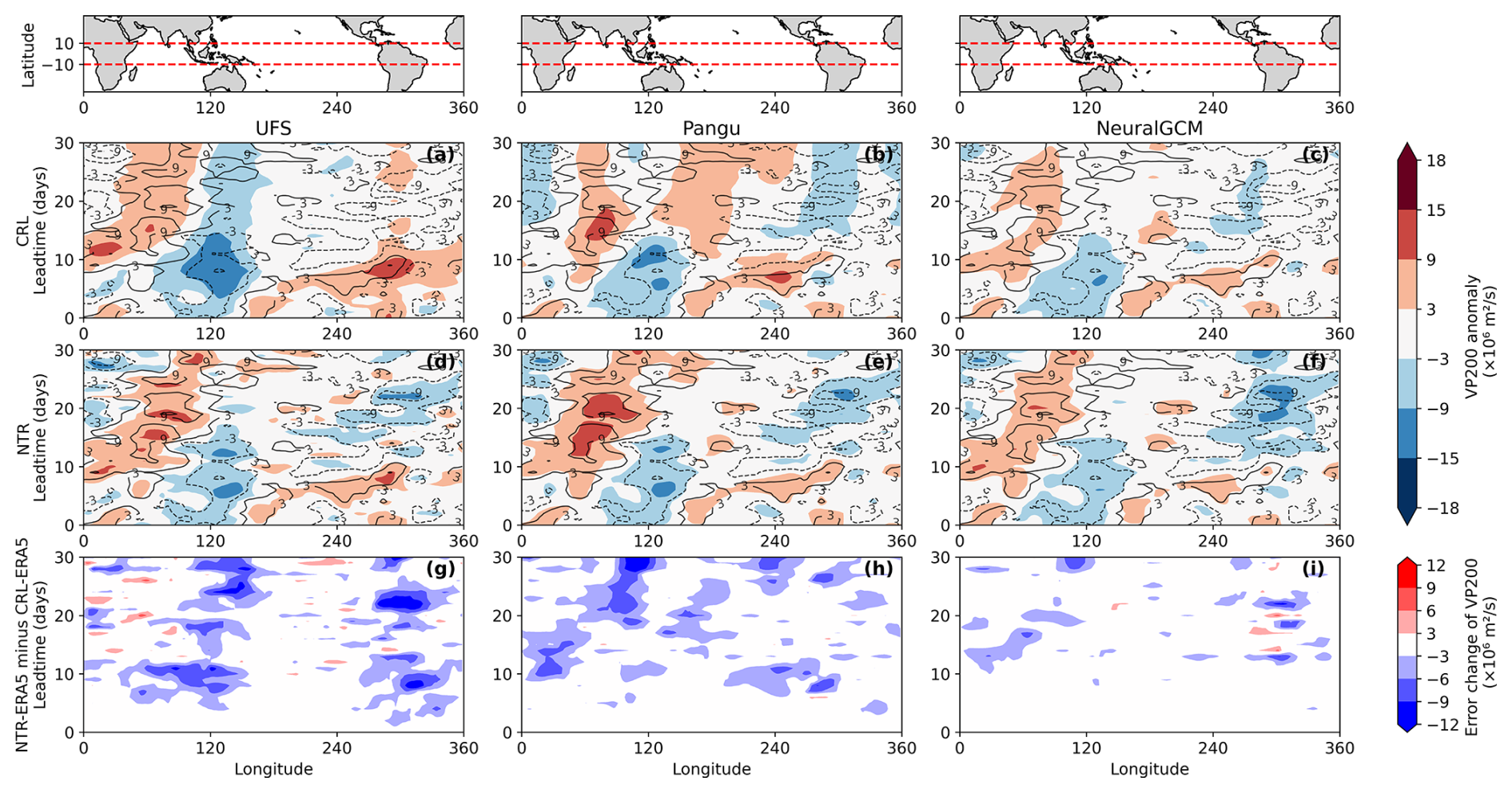
Figure 4 Time-longitude diagrams of ensemble-mean 200 hPa velocity potential anomaly (10⁶ m² s⁻¹ in shading) from CRL (a–c) and NTR (d–f) initialized on 15 December 2022 for UFS (a, d), Pangu-Weather (b, e), NeuralGCM (c, f). The ERA5 velocity potential anomaly is shown in black contours (at −9, −3, 3, 9 × 10⁶ m² s⁻¹, positive in solid, negative in dashed) from (a) to (f). $\mathrm{|}\mathrm{NTR}-\mathrm{ERA}\mathrm{5}\mathrm{|}-\mathrm{|}\mathrm{CTL}-\mathrm{ERA}\mathrm{5}\mathrm{|}$ (shading) for UFS (g), Pangu-Weather (h) and NeuralGCM (i).

The NTR experiments in UFS exhibits large differences in terms of RWS relative to CRL (Fig. 3a, d, and g) over eastern Asia and the western Pacific. UFS NTR shows an improved RWS with a smaller forecast error (MAE: 0.59). The differences in Rossby wave source emerge as a negative–positive couplet in 200 hPa relative vorticity in this region indicating a slight eastward shift of the broad trough–ridge pattern over eastern Asia and the western Pacific (Fig. 3j, Moore et al., 2026).

Pangu-Weather and NeuralGCM CRL exhibit a better prediction of the RWS associated with the divergent outflow with an MAE of 0.80 and 0.90, respectively (Fig. 3b and c). In NTR, RWS is strengthened in the northeastern Indian ocean for both MLWP models (Fig. 3e and f). Overall, the reduction of the MAE through tropical relaxation is considerably smaller than in UFS (Fig. 3d, e, and f). The differences in RWS manifest as dipoles of vorticity differences along the strongest vorticity gradient (Fig. 3k and l). However, the dipoles are considerably weaker than between CRL and NTR in UFS.

To further understand the role of the tropical forcing for the predictability of the event, we specifically focus on the representation of the velocity potential (VP) associated with the MJO. As outgoing long-wave radiation (OLR) is not available from the models used here, we use 200 hPa VP anomalies as a proxy for the convective activity associated with the MJO. Time–longitude Hovmöller diagrams averaged between 10° S–10° N are shown in Fig. 4.

Starting with ERA5 (black contours in Fig. 4), the period is characterized by suppressed convection over the Indian Ocean after day 10 and slightly enhanced convection over the Maritime continent most noteworthy between 5 to 15 d lead time. Though the suppressed convection and its eastward propagation can be seen in the CRL experiment with UFS, the convective activity is substantially overestimated over the Maritime Continent (Fig. 4a) which is consistent with the too strong RWS. Pangu-Weather and NeuralGCM are both characterized by a weaker dipole pattern in 200 hPa VP with the magnitude of the negative VP over the Maritime Continent being closer to that in ERA5 (Fig. 4b and c).

All NTR experiments clearly represent the suppressed convective activity over the Indian Ocean from day 10 onwards (Fig. 4d–f). Likewise, all 3 models show error reduction and better represent the 200 hPa VP anomaly over the Maritime Continent (Fig. 4g–i). Most notable is the reduced magnitude of the VP in UFS between 5 and 30 d forecast lead time. For Pangu-Weather and NeuralGCM, the negative 200 hPa VP is of similar magnitude as in CRL, but the representation of the occurrence of local and temporal maxima is improved after relaxation. Overall, the changes in 200 hPa VP indicate an improved representation of the MJO envelope, which likely contributes to a better representation of the tropical–extratropical teleconnection.

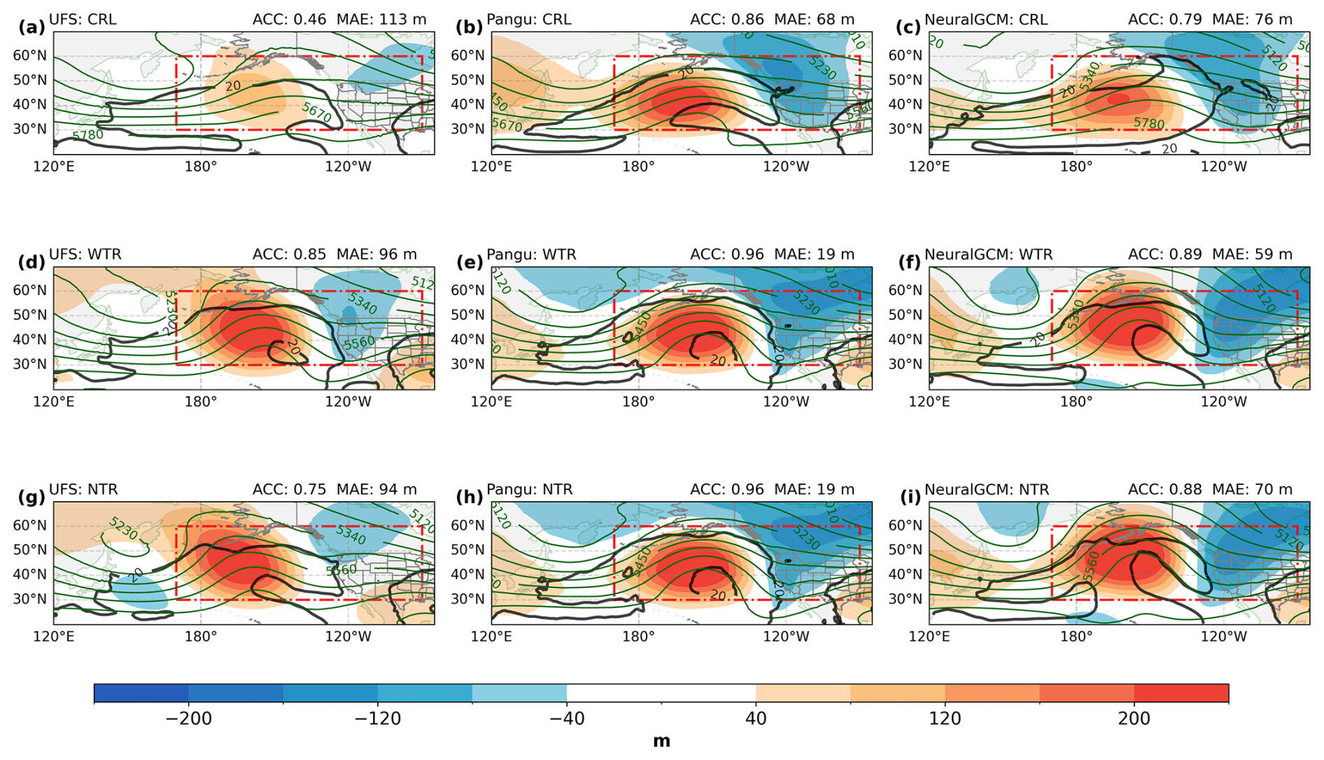
Figure 5 Same as Fig. 2, but for forecasts initialized on 2 February 2023. The 20 $\mathrm{g}{\mathrm{kg}}^{-\mathrm{1}}\mathrm{m}{\mathrm{s}}^{-\mathrm{1}}$ isoline for moisture transport is shown in bold black.

3.2 Case study 2: February to March 2023

For the second event from mid February to the beginning of March 2023, the ERA5 accumulated precipitation over California reaches approximately 200 mm (Fig. 1c). Though the MJO entered simultaneously its active phases 6–7, the midlatitude geopotential height anomalies are very different from case 1. For case 2 (valid from 17 February–3 March), a persistent positive geopotential height anomaly is located over the eastern North Pacific (Fig. 1d). ARs are deflected around the associated high pressure anomaly and reach the west coast of North America in a northwesterly flow. There, the precipitation is connected to the passage of several upper-level troughs (as manifested by a negative geopotential height anomaly in Fig. 5) associated with Rossby wave breaking on the eastern flank of the Pacific ridge.

All 3 models exhibit greater subseasonal forecast skill in the CRL experiment (Fig. 5a–c) with higher ACCs and lower MAEs than for Case 1. Pangu-Weather especially depicts the positive geopotential height anomaly over the eastern North Pacific and the surrounding moisture transport, whereas UFS and NeuralGCM underestimate the anomaly amplitude, resulting in lower ACC and higher MAE.

In the UFS model, both the WTR (Fig. 5d) and NTR (Fig. 5g) experiments yield a substantially stronger ridge over the eastern North Pacific, resulting in a considerably improved representation of the large-scale circulation compared to the CRL experiment (Fig. 5a). This finding is consistent with Moore et al. (2026). Pangu-Weather shows modest improvements for the WTR (Fig. 5e) and NTR (Fig. 5h) experiments, particularly in capturing the positive and negative geopotential height anomaly patterns. NeuralGCM predicts a pattern similar to the UFS model, yet with overall higher forecast skill than UFS in this case (cf. Fig. 5a, d, and g vs. Fig. 5c, f, and i). The bands of highest moisture transport around the ridge over the eastern North Pacific, with magnitudes around 40 $\mathrm{g}{\mathrm{kg}}^{-\mathrm{1}}\mathrm{m}{\mathrm{s}}^{-\mathrm{1}}$, are consistently well represented. Independent of the relaxation configuration, the forecasts for Pangu-Weather and NeuralGCM with relaxation yield significantly improved representation of the location, amplitude and positive tilt of the trough near the west coast of North America, which may affect precipitation. The UFS forecasts only show a modest improvement regarding the location of the trough.

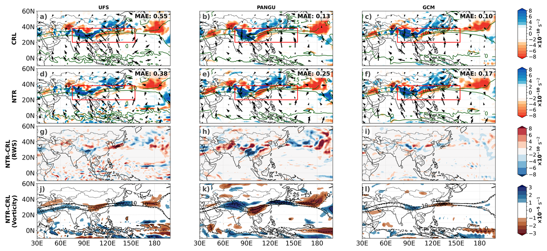
Figure 6 Comparison of ensemble-mean forecasts from CRL (a–c) and NTR (d–f) averaged for 9–15 February 2023, same as Fig. 3.

The improvements in large positive geopotential height anomalies in the UFS for both WTR and NTR indicate that tropical forecast errors in this model exert a strong influence on predicting the blocking ridge over the eastern North Pacific, even if they did not strongly constrain predictions of downstream wave breaking and trough amplification near the west coast of North America. In the UFS WTR experiment, positive height anomalies are well captured, but negative anomalies near the west coast of North America remain misrepresented. Interestingly, MLWP models better capture the positive geopotential height anomaly over the eastern North Pacific in the CRL without relaxation, possibly due to superior representation of tropical conditions and Rossby wave forcing even without nudging.

Overall, the differences in forecast skill between the WTR and NTR experiments are remarkably small across all 3 models (cf. Fig. 5d–f and 5g–i). This similarity suggests that forecast skill is not highly sensitive to the width of the tropical nudging region. In other words, extending the nudging region beyond the core tropics does not substantially influence the forecast evolution, implying that forecast errors originating in the deep tropics likely play the dominant role in this event. However, this result does not imply that subtropical or extratropical processes are unimportant, but rather that constraining the large-scale tropical state appears sufficient to capture the key sources of predictability in this case.

We also examine the RWS to assess the impact of the tropical relaxation during week 2 on the forcing of the extratropical wave response. The UFS overestimates the RWS over eastern Asia and the western Pacific in CRL (Fig. 6a; Moore et al., 2026) relative to NTR (Fig. 6d), reflecting an overprediction of the divergent outflow and negative vorticity advection in that region. The error in the RWS is reduced when NTR is applied, with the MAE decreasing from 0.55 to 0.38.

Results of Moore et al. (2026) suggest that an improved representation of the RWS in NTR relative to CRL led to a better representation of the extratropical pattern over the North Pacific in this case. Pangu-Weather and NeuralGCM exhibit a dipole pattern in terms of RWS over Eastern Asia in the CRL experiment with lower MAEs (Fig. 6b and c). Meanwhile, in the NTR experiments, the RWS in both MLWP models is even slightly deteriorating (Fig. 6e and f). Higher MAEs in NTR than in CRL are aligned with the hypothesis above that the divergent outflow from the tropics in Case 2 is likely better represented in the MLWP models than in UFS. Finally, there is a noteworthy area of intense positive RWS and divergent winds over the eastern Pacific, which is possibly linked to enhanced warm conveyor belt activity in this mid-latitude region following MJO phases 6 and 7 (Quinting et al., 2024).

NeuralGCM reaches the lowest RWS MAE in the CRL experiment (0.10). This indicates that the model already captures most of the contributing RWS during the early stage without any nudging. Moreover, the differences in RWS and ζ between the CRL and NTR are comparably small (Fig. 6i and l), indicating that NeuralGCM's representation of the relevant dynamical fields is less sensitive to the relaxation procedure.

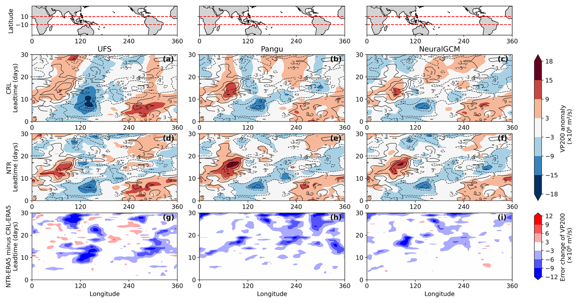
Figure 7 Time-longitude diagrams of ensemble-mean 200 hPa velocity potential anomalies, initialized on 2 February 2023. Same as Fig. 4.

To investigate potential changes in the tropics through the relaxation, we analyze anomalies of the 200 hPa VP (Fig. 7). As for Case 1, the situation is characterized by a dipole of VP anomalies over the Indian Ocean and the Maritime Continent (black contours). The negative 200 hPa VP anomaly (Fig. 7a) is overestimated and longer lived in the UFS CRL relative to ERA5. The magnitude and timing of the negative 200 hPa VP anomaly are considerably better represented in Pangu-Weather and NeuralGCM already in the CRL (Fig. 7b and c). Accordingly, the improvements of the negative 200 hPa velocity potential anomalies in NTR in Pangu-Weather and NeuralGCM are rather small (Fig. 7e, h, f, and i). In contrast, relatively large improvements are found in the NTR experiments of UFS near the western and eastern Pacific (Fig. 7d and g). This is consistent with the large improvements in the representation of 200 hPa RWS and geopotential height anomalies when tropical relaxation is applied in UFS.

3.3 Synthesis of both cases: forecast uncertainty

Given the different impacts of relaxation in the 2 cases and the varying contribution of individual members to the ensemble mean, we further examine forecast skill per ensemble member. This provides a more detailed view of forecast performance and model uncertainty across the ensemble for each case.

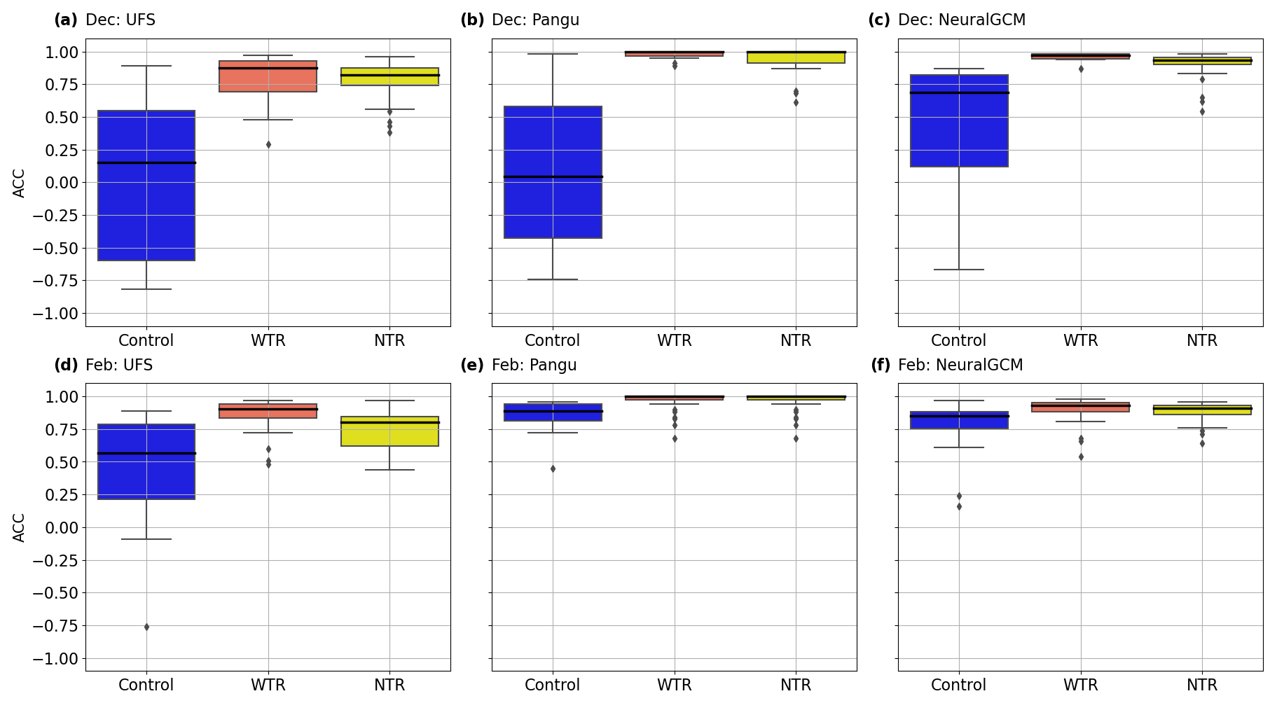
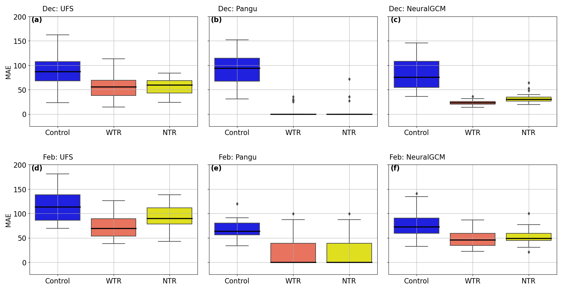
Figure 8 Distribution of the 500 hPa geopotential height latitude-weighted centered ACC values for all 30 ensemble members in different relaxation experiments for weeks 3–4. The horizontal line denotes the median, boxes give the 25th to 75th percentile range, whiskers denote the smallest and largest values within 1.5 times the interquartile range, and outliers are given by black dots. Results are shown for the (a, d) UFS, (b, e) Pangu-Weather, and (c, f) NeuralGCM for (top) the December case and (bottom) the February case.

Both MLWP models demonstrate on average a higher forecast skill in the CRL experiment for the December case compared to UFS (Figs. 8a–c; A4). Still, individual ensemble members in Pangu-Weather and NeuralGCM show negative ACC and thus no forecast skill for this particular event. The application of tropical relaxation (WTR) in December leads to a clear improvement over the control experiment, suggesting a strong influence of tropical forecast errors in all 3 models on the mid-latitude prediction skill. The substantially reduced range of ACC values between the different ensemble members can be attributed to the reduced variability in the tropics through tropical relaxation.

In contrast to the December case, the February case shows less sensitivity to tropical relaxation (Fig. 8d–f) and is better captured by all 3 models in CRL, especially for the MLWP models. Though a large improvement in terms of ACC can be seen for UFS, the median ACC of Pangu-Weather and NeuralGCM increases only marginally when tropical relaxation is applied. Also, the smaller range of ACC values between the different ensemble members suggest a higher confidence in the predictions of the 2 MLWP models. The rather small improvement through tropical relaxation compared to the December case further suggests that tropical forecast errors in MLWP models are less critical for the predictability of the February precipitation event, especially during weeks 1–2 (Fig. 7). Errors in the tropics in UFS seem relatively large and might be associated with parameterization of physical processes that affect the representation of tropical convection.

Another possible explanation for the weaker impact of the relaxation in the February event is the different state of tropical variability at initialization. In the December case, the MJO is not active at initialization, whereas in the February case the MJO is already active in phase 3 (Moore et al., 2026). An active MJO provides a coherent large-scale tropical signal that can enhance subseasonal predictability and may already be reasonably represented in the initial conditions. As a result, the February forecasts may contain higher intrinsic predictability in the tropics, reducing the additional benefit from relaxation. Overall, our result indicates that other regions provided predictability for the February case, which could be further investigated with additional nudging experiments in a future study.

4 Conclusion

This study evaluates the impact of tropical relaxation in UFS, Pangu-Weather and NeuralGCM for 2 case studies of long-duration precipitation events in United States West Coast following MJO activity over the Maritime Continent and the western Pacific. Our 3 central findings are the following.

• For 500 hPa geopotential height, the forecast skill of the CRL experiment with Pangu-Weather and NeuralGCM exceeds that of the UFS. These findings underscore the promise of data-driven models in subseasonal forecasting, particularly given their lower computational costs. Recent work by Peings et al. (2026) has also provided a systematic evaluation of S2S forecast skill over the North Pacific/Western North America region, showing that 2 MLWP models (SFNO-HENS and NeuralGCM) exhibit skill comparable to ECMWF for MJO-related and North Pacific atmospheric teleconnection patterns during the October–March season. A limitation of this study is its focus on only 2 events with substantially different dynamics and predictability. Thus, further systematic evaluations across multiple years and a broader range of events are still needed to fully assess the generalizability of these results.

• Relaxation experiments on the subseasonal timescale can be stably conducted in MLWP models, at considerably reduced computational costs in comparison to NWP models. The reference experiments with an NWP model prove useful to establish the necessary confidence in the MLWP relaxation approach at subseasonal scales. Relaxing tropical fields improves forecast skill in MLWP models as in the NWP model. For example, in the December case, tropical relaxation corrects the moisture transport towards western North America in all 3 models. This suggests that a better representation of the tropical atmospheric state in the models would have improved the prediction of this particular event. Further consistent behaviors are the reduction of the range of ACC values between the different ensemble members and a better representation of Rossby wave source one week earlier. This suggests that the MLWP models used here follow a physically consistent way in generating the Rossby wave.

• The impact of tropical relaxation on mid-latitude forecasts varies between cases. In the December case, forecasts improve substantially in all 3 models, suggesting that key tropical processes driving the teleconnection are poorly captured. In the February case, improvements are smaller, particularly for the MLWP models, likely due to a combination of better tropical representation in the control runs and a reduced tropical influence on the event, as also noted by Moore et al. (2026). Additional experiments with relaxation of the stratosphere or high latitudes would be necessary to reveal the importance of other regions for the predictability of the event.

In general, the higher forecast skill in NeuralGCM and Pangu-Weather compared to UFS suggests that the NWP model does not fully exploit the predictability inherent in these 2 events. Identifying which relaxation configurations most strongly affect forecast skill will help understand these mechanisms, ultimately guiding targeted improvements in future forecasting systems. Improving the representation of the tropics will likely enhance extratropical prediction skill for similar cases, although a systematic analysis is needed in specific regions to identify where tropical improvements yield the greatest benefit. To translate this insight into improved forecast skill, future research should diagnose the origin of large-scale anomalies, particularly, the pathways through which tropical variability influences the extratropical circulation, and assess how predictable these processes are in MLWP models. Such targeted relaxation experiments could also guide MLWP and NWP development by revealing which regions or processes affect forecast skill most significantly.

To conclude, our results suggest that improving the representation of the tropical atmospheric state can enhance subseasonal-to-seasonal (S2S) forecast skill. While first-generation machine learning weather prediction (MLWP) models are typically trained using a mean-squared error (MSE) loss function, this approach tends to penalize large deviations and favour smooth solutions, which can lead to an underestimation of variability – often referred to as the “loss of activity” problem (Bouallègue, 2024). As a result, important features of tropical variability, such as convective activity and wave dynamics, may be insufficiently represented. More recent developments in loss function design aim to better capture variability and extremes. Such advancements could lead to improvements in MLWP model representation of variability in the tropics and, in turn, improved predictions in the midlatitudes.

Although intrinsic limits of tropical predictability exist (Judt, 2020), the tropics exhibit a substantially longer predictability horizon than the extratropics, suggesting considerable scope for improvement. In this context, recent studies indicate that MLWP systems may more effectively exploit this intrinsic predictability and can even extend the forecast skill of numerical weather prediction (NWP) models when used in a coupled or nudged framework (Polichtchouk et al., 2026). These developments highlight the potential of MLWP systems to complement traditional NWP models and further advance S2S forecasting skill.

Appendix A

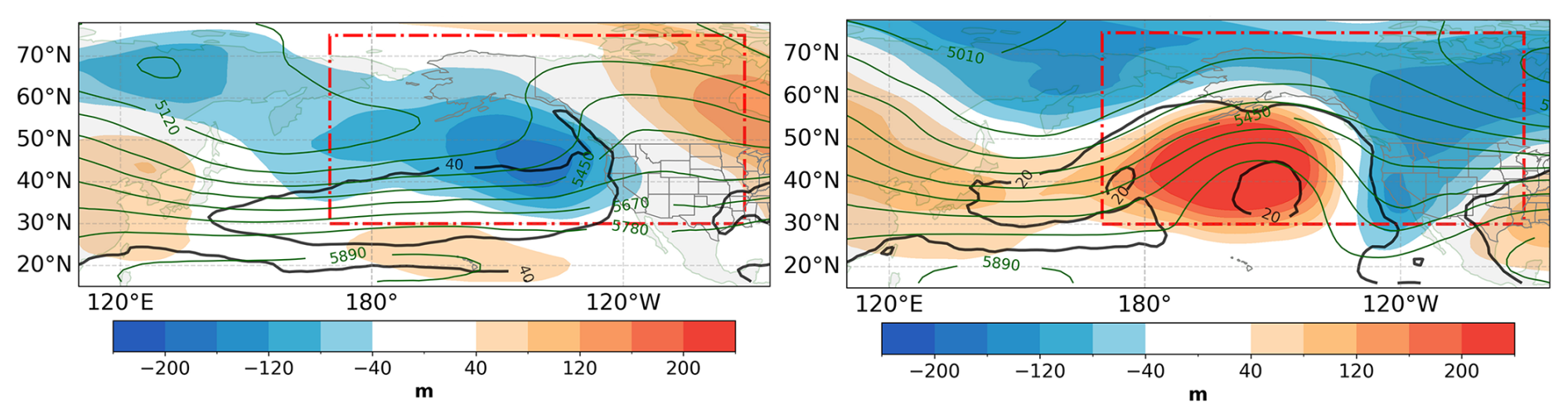
Figure A1 Same as Fig. 1 b and d, but showing NeuralGCM replay with the fixed SST forcing for Case 1 (Left) and Case 2 (Right).

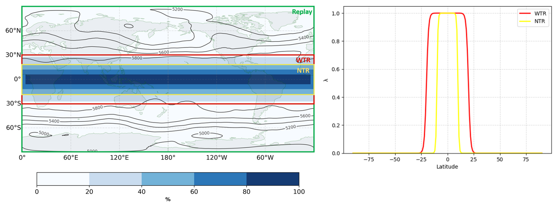
Figure A2 Visualization of relaxing regions during the forecasts for different experiments (Left) and λ as a function of latitude for WTR and NTR (Right). Shading in the right panel showing relaxation area in the WTR experiment as an example.

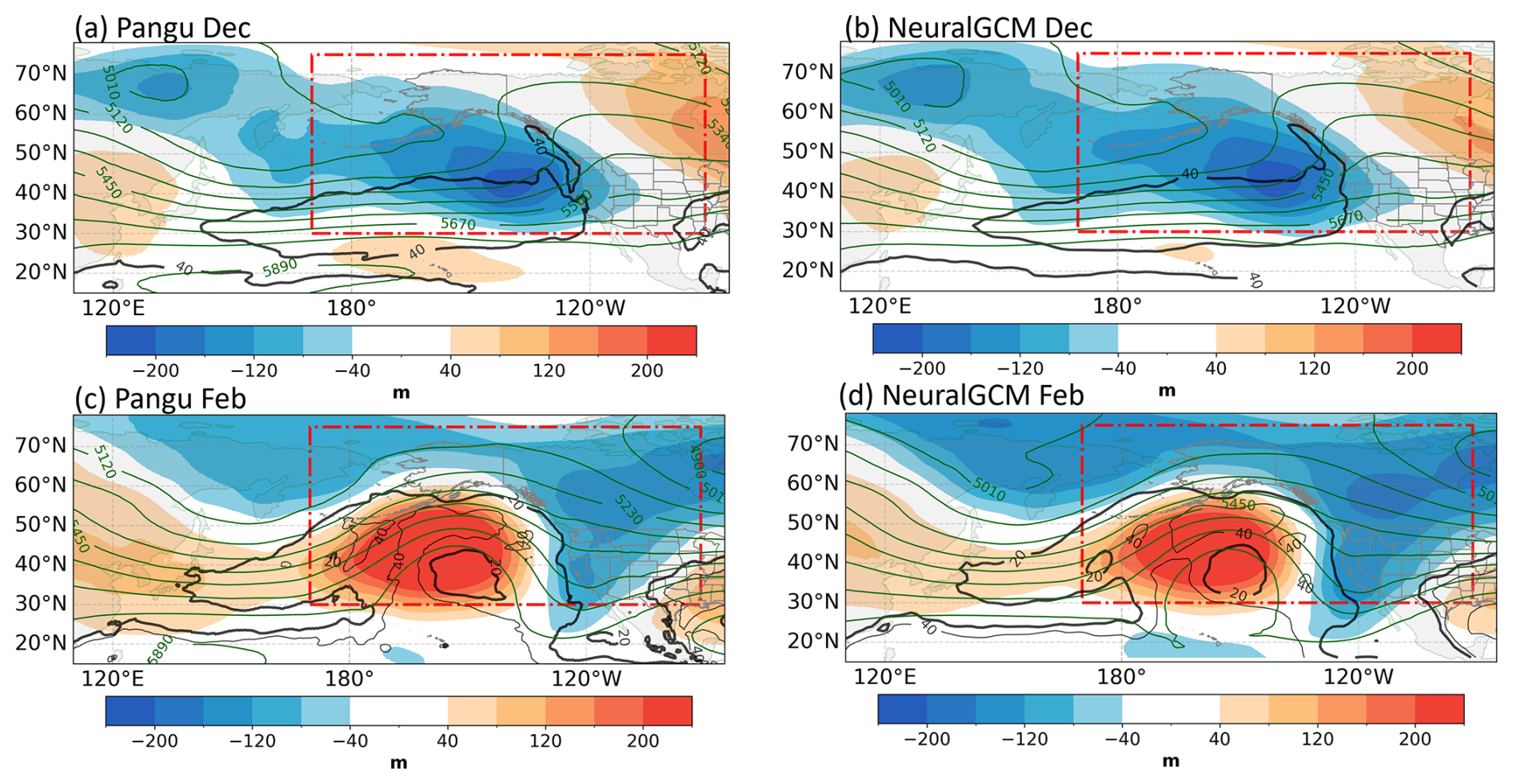
Figure A3 Same as Fig. 1b and d, but showing model replay with (a, c) Pangu-Weather and (b, d) NeuralGCM.

Figure A4 Same as Fig. 8, but showing MAEs in units of m.