Cold spells induced by slow-moving and amplified large-scale ridge and trough

Cold spells in the Northern Hemisphere mid-latitudes have been linked to Rossby waves. Yet the mechanisms by which these large-scale waves impact cold-spell formation remain unclear. Here we develop novel metrics to separately determine the amplitude and speed of large-scale ridges and troughs, derived from the first five zonal Fourier decompositions of the geopotential height field. This approach allows us to examine the behavior of large-scale ridges and troughs during winter cold spells. These ridges and troughs mainly represent climatological features, which can be regarded as wobbling around their climatological positions due to interactions with background flow. Our findings indicate that while ridges and troughs across the entire mid-latitudes experience significant changes during cold spells, the local ridge and trough near the cold spell's location play a major role in the development of these events. The nearest upstream ridge and downstream trough of the cold-spell region are located in a way that facilitates development of the extreme cold anomaly. This ridge and trough amplify and slow down, enhancing and prolonging southward advection of cold air from the Arctic into the cold-spell region. The slow and amplified upstream ridge and downstream trough occur several days before the region’s minimum temperature, suggesting these local wave anomalies induce cold-spell formation.

1 Introduction

High-amplitude quasi-stationary Rossby waves may generate extreme weather events (e.g., Hoskins and Woollings, 2015; Fragkoulidis and Wirth, 2020; White et al., 2022), and an increase in temperature extremes in the mid-latitudes is argued to be linked to increased upper-atmosphere waviness (e.g., Fragkoulidis et al., 2018). An increase in meridional amplitude of Rossby waves may enhance the meridional exchange of warm and cold air, leading to the advection of cold air to the south and warm air to the north (Zschenderlein et al., 2018; Jolly et al., 2021). Some studies linked extreme temperatures to a significant amplified circumglobal waviness based on wave amplitudes of individual wave numbers (Petoukhov et al., 2013; Screen and Simmonds, 2014), while others asserted a robust correlation between local waviness and temperature extremes (Röthlisberger et al., 2016; Fragkoulidis et al., 2018; Fragkoulidis and Wirth, 2020). Studies based on the amplified circumglobal waviness argued that free-traveling synoptic waves of some specific wave numbers (6, 7, or 8) may be trapped within the midlatitude waveguide, leading to extreme temperature events (Petoukhov et al., 2013; Kornhuber et al., 2017), whereas others caution against overemphasizing the significance of circumglobal waviness, suggesting that local climatic factors may play a more critical role in influencing temperature extremes (Teng and Branstator, 2019).

Slow movement of Rossby waves may also lead to weather persistence, for instance, in terms of blocking, which may develop into extreme weather events, such as floods, droughts, heat waves, and cold spells (Francis and Vavrus, 2012; Pfleiderer and Coumou, 2018; Riboldi et al., 2020; Jolly et al., 2021; Wicker et al., 2024). Extreme rainfall over Eastern Australia has been linked to slow-moving upper-level low-pressure systems (Barnes et al., 2023; Reid et al., 2025; Vries et al., 2025), and it is argued that slow propagation of atmospheric blocking, identified using a blocking cell-tracking algorithm, leads to significant surface temperature anomalies (van Mourik et al., 2025). The propagation speed of atmospheric blocking can impact the upstream and downstream of the block in the way that rapidly westward-moving blocks lead to less persistent cold events in the upstream of the block, while slower westward-moving blocks lead to strong cold anomalies in the downstream of the block (Chen and Luo, 2017; Yao et al., 2017).

The frequency of extreme events has risen in recent decades due to anthropogenic warming (IPCC; Seneviratne et al., 2021), and these events are likely to become more intense and break the previous extreme records by a large margin in the following decades (Fischer et al., 2021). Despite the warming Earth, cold spells in some regions of the Northern Hemisphere have recently increased (e.g., Cohen et al., 2021, 2024), although, in general, cold spells are projected to become less frequent by the end of the century (IPCC; Seneviratne et al., 2021), and the likelihood of experiencing the strongest historical extreme cold spell events is expected to diminish (Ribes et al., 2025).

Increases in extreme event frequency, specifically cold spells, have been linked to Arctic amplification (AA), a phenomenon by which the Arctic warms faster than the mid-latitudes (e.g., Francis and Vavrus, 2012; Cohen et al., 2014; Graversen et al., 2025): the AA is weakening the jet stream, making the large-scale atmospheric waves more wavy (Francis and Vavrus, 2012; Coumou et al., 2015; Stendel et al., 2021); in addition, AA causes Rossby waves to become more stationary, resulting in an increase in the frequency of extreme weather (Francis and Vavrus, 2012). This hypothesis, however, has been questioned by several studies (e.g., Barnes, 2013; Screen and Simmonds, 2013; Hassanzadeh et al., 2014; Blackport et al., 2022, 2024). In addition, a recent study suggests that the poleward expansion of the tropics can reduce the frequency of persistent mid-latitude heat waves by shifting storm tracks and increasing phase speeds (Wicker et al., 2025).

The dispute about the influence of the AA on planetary waves might stem from the sensitivity of waviness assessments to the applied metric (Geen et al., 2023), which emphasizes the importance of evaluating a broader range of wave metrics. However, existing wave amplitude metrics, such as Rossby wave packets (e.g., Fragkoulidis et al., 2018; Röthlisberger et al., 2019), local jet waviness (e.g., Röthlisberger et al., 2016), and hemispheric variability (e.g., Petoukhov et al., 2013; Kornhuber et al., 2019), do not capture the role of the amplitude of each ridge and trough in temperature events. In addition, as far as the authors know, the speed of local ridges and troughs and their role in extreme events have not earlier been quantified. Some studies estimate atmospheric phase propagation by following grid points using lag-correlation in different bandpass-filtered geopotential height maps, tracking the maximum positive correlation center (e.g., Blackmon et al., 1984; Takaya and Nakamura, 2001). Others derive phase-speed spectra for each zonal wavenumber by performing a space–time spectral decomposition of upper-tropospheric winds along latitude circles (e.g., Randel and Held, 1991; Domeisen et al., 2018; Riboldi et al., 2020). A local approach has also been applied to estimate the speed of Rossby wave packets (e.g., Fragkoulidis and Wirth, 2020; Fragkoulidis, 2022). Here, we aim to explore the linkage between cold spells, in particular those that are associated with the advection of cold air from the Arctic, and the amplitude and speed of large-scale ridges and troughs in the vicinity of cold spells. Cold spells are particularly of interest in the context of Rossby waves because these cold extremes are argued to be primarily driven by the large-scale advection of cold air from higher latitudes (Bieli et al., 2015; Harnik et al., 2016; Tuel and Martius, 2024; Mayer, 2025). However, in some regions, especially near the Arctic and Antarctic, diabatic processes are considered to play the dominant role in driving cold extremes (Röthlisberger and Papritz, 2023).

This article is organized as follows. Section 2 describes the study regions, the data used, and the definition of cold spells. Section 3 introduces the newly developed wave metrics. Section 4 presents the application of the wave metric to cold spells, demonstrating its effectiveness. Finally, Sect. 5 provides the conclusions and discusses the implications of the findings.

2 Study regions, data, and cold-spell definition

In this study, we used the European Centre for Medium-Range Weather Forecasts (ECMWF) analysis 5th Generation (ERA5) dataset with a horizontal resolution of 0.25° × 0.25° (Hersbach et al., 2020) for the period 1978–2024. The study is for the winter season (December–January–February) and the satellite era. Minimum daily temperature and daily average temperature are obtained based on hourly ERA5 data. Additionally, 3-hourly geopotential height (gph) data at 300, 500, and 850 hPa are utilized.

2.1 Cold spells

To identify cold spells and their magnitudes, the cold wave magnitude index daily (CWMId; Morlot et al., 2023) is applied at each horizontal grid point. The daily cold spells index is based on at least 3 consecutive days below a daily threshold, defined as the 10th percentile of anomalies relative to the climatology of minimum daily air temperature smoothed with a 31 d running mean filter. The climatology is based on the reference period 1981–2020. The background trend is small relative to the daily anomalies, and we have verified that it does not affect the overall conclusions drawn in the paper (not shown).

2.2 Study regions selection

To select cold spell regions, we first identified historical winter extreme 2 m temperature days on the hemispheric scale. To do so, a non-standardized version of the mid-latitude extreme (MEX; Riboldi et al., 2020) index is applied for land in four latitude bands (35–45, 45–55, 55–65° N, and the entire mid-latitudes: 35–65° N). Dividing the mid-latitudes into three sub-bands enables an identification of extreme cold days in the southern, central, and northern sections of the mid-latitudes. The MEX provides an overall measure of mid-latitude temperature daily variance by averaging over each grid point in the mid-latitudes the squared anomaly of the temperature. Here, “non-standardized” means the MEX index is used without subtracting its time-averaged mean and dividing by its standard deviation, as done in Coumou et al. (2014). The top 1 % of daily MEX values – a criteria to classify cold extreme days – within all the winters during the period 1978–2024 yields 125, 117, 119, and 141 d for the bands 35–45, 45–55, 55–65, and 35–65° N, respectively. To identify the areas providing the largest cold anomaly contribution to the top 1 % MEX days of each latitude band, the CWMId (Fig. 1) and temperature anomaly (Fig. S1 in the Supplement) of the extreme temperature days are calculated at each grid point in the mid-latitudes. Since these two diagnostics yield similar results, we focus on CWMId in the analysis.

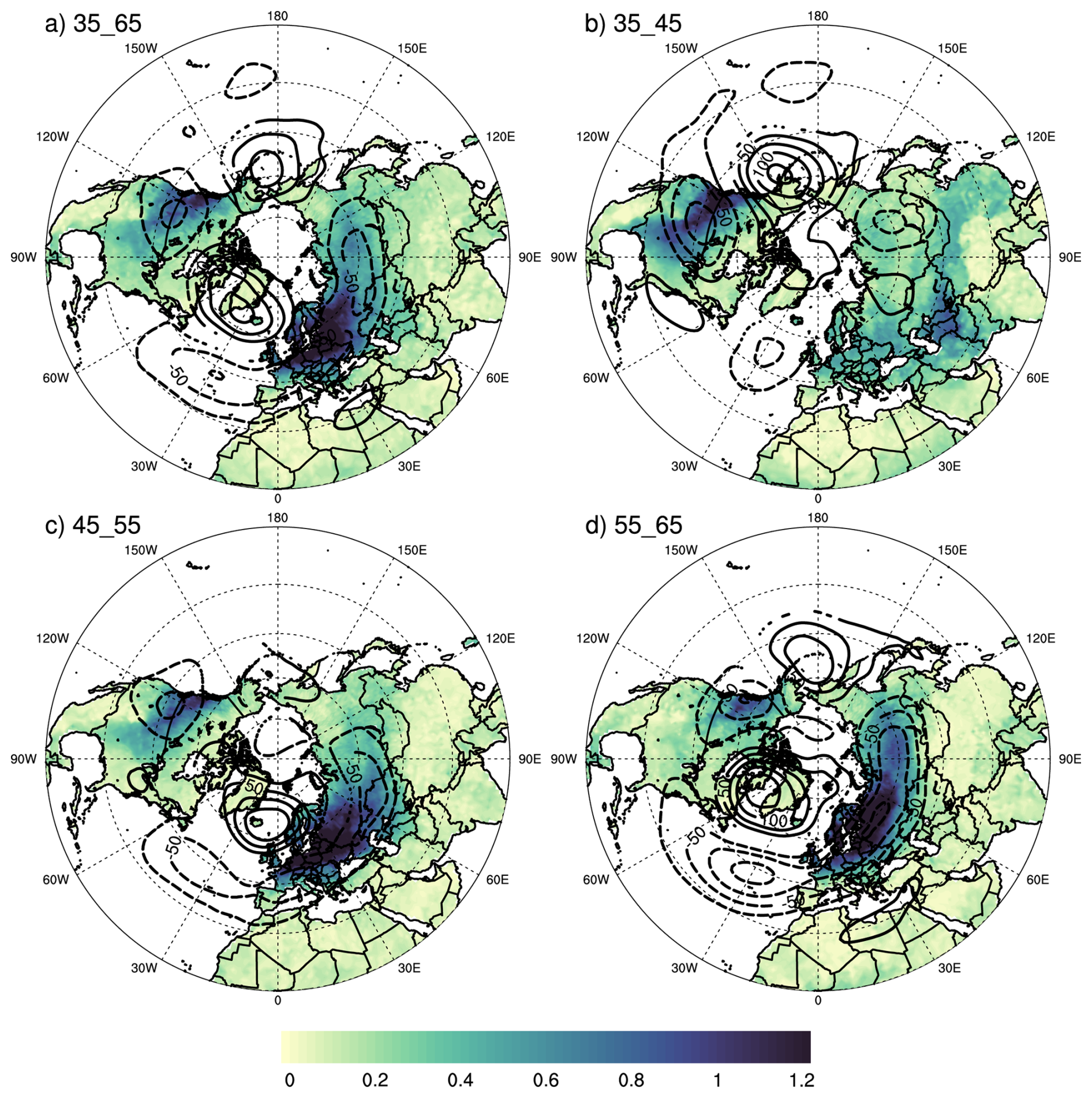
Figure 1 The composite of the geopotential height anomaly relative to climatology (m) at 500 hPa (lines; only significant at the 95 % confidence level) and the cold wave magnitude index daily (CWMID; colors) for cold extreme days given by the top 1 % of the MEX over land at the latitude band of (a) 35–65° N, (b) 35–45° N, (c) 45–55° N, and (d) 55–65° N.

Figure 1 shows the composite of the gph anomaly at 500 hPa and the cold-wave magnitude index for cold extreme days for each latitude band. For the top 1 % MEX days over the whole midlatitude (35–65° N; Fig. 1a), cold spells are more intense in the northwestern part of North America and northwestern Eurasia. The intensity decreases toward the south and east in both continents. The gph anomaly is positive over Greenland and the North Pacific Ocean, the two primary blocking regions (Barriopedro et al., 2006). Over the North Atlantic Ocean, a negative gph anomaly is encountered that may indicate the negative phase of the North Atlantic Oscillation during these cold events, a phenomenon that promotes European winter cold spells (e.g., Hanna and Cropper, 2017; Vihma et al., 2020).

For the top 1 % MEX days over 35–45° N, little or no positive gph anomaly is encountered over Greenland, which is consistently associated with a weak intensity of CWMId over Europe (Fig. 1b). The main gph anomaly consists of a positive height anomaly over Alaska and a negative height anomaly downstream over West North America. Consistently, in this latitude band, CWMId is more pronounced over northwest North America, the central US, and Central Asia. Intense CWMId over Central Asia appears to differ from that of the central US, as it is likely not linked with higher latitudes, leading us to speculate that the cold spells in this region do not originate from Arctic cold air. Therefore, this region is not included in our study.

For the top 1 % MEX days over 45–55° N, in contrast to 35–45° N, there is a strong positive gph anomaly upstream of Europe, centered over Iceland, while the positive gph anomaly is weak upstream of North America (Fig. 1c). For this latitude band, the CWMId is strong over the middle and east of Europe and over the west of Canada. For the top 1 % MEX days over 55–65° N, CWMId is stronger at higher latitudes, encompassing Scandinavia, the west of Canada, and Northern Siberia (Fig. 1d). For this latitude band, there are two strong positive gph anomaly centers over Baffin Bay and the Bering Sea. The top 1 % MEX over the 45–55 and 55–65° N, similar to MEX across the entire midlatitude, exhibits a negative gph anomaly over the North Atlantic Ocean.

Based on the results of the composite of days with the top 1 % MEX over these four latitude bands, 9 regions are selected for the study of the impact of large-scale upper atmospheric circulation on cold spells, shown as hatched areas in Fig. 2. The regions include Northwest Canada (R01), Northwest US and Southwest Canada (R02), Central US (R03), British Isles (R04), Scandinavia (R05), Europe (R06), Northwest Russia (R07), Southwest Russia (R08), and Northern Siberia (R09). If 50 % or more of the grid points within each region experience cold spells on a given day, it is considered a cold spell day in that region. Applying grid-point thresholds between 20 % and 70 % are also tested to ensure that the drawn overall conclusions remain unchanged for an altered threshold. The number of days with 50 % or more of the grid points experiencing cold spells in each region, as based on the CWMId, is 239, 184, 164, 157, 170, 171, 195, 150, and 152, respectively, for R01 to R09.

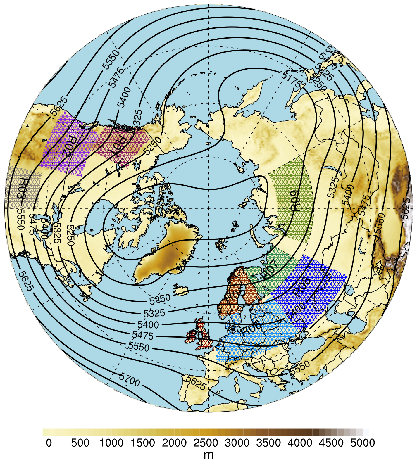
Figure 2 The chosen study regions (hatches). The winter climatology mean geopotential height field (m) and the elevation above mean sea level (m) are shown by contours and shading, respectively.

The MEX metric may be somewhat biased because it accounts for both warm and cold anomalies. The simultaneous occurrence of cold anomalies in Eurasia and Northwest America, alongside warm anomalies in Greenland and Beringia, might have contributed to a higher MEX value for the selected days (see Fig. S1). Nevertheless, our selected regions cover all of Europe and the western part of North America, with the only significant area not included in our analysis being the eastern part of North America, which could be addressed in future research.

2.3 Significant test

To test the null hypothesis that anomalies associated with the cold spells are zero, a Monte Carlo simulation with random samples is employed. Specifically, the average number of cold spell days across each region is compared with the average of an equivalent number of randomly selected days. Instead of selecting random days from the entire winter season, the selection is weighted based on the frequency distribution through the season of cold spell days, since cold spells appear to occur more frequently in some parts of winter. This Monte Carlo test is repeated at least 2000 times to ensure a sufficient sample size, and significant differences from zero are identified at the 95 % confidence level.

3 Wave metrics

3.1 Trough and ridge speed

To enhance the trackability of atmospheric waves, a zonal Fourier decomposition of the gph field is employed to separate it into distinct harmonic waves based on the zonal wave number. The combination of the first five waves captures the large-scale ridges and troughs of atmospheric waves (Z1–5; see the solid line in Fig. 3a for an example). These ridges and troughs represent planetary waves in low latitudes and both planetary and synoptic-scale waves in high latitudes. The longitude position of these ridges and troughs at high latitudes aligns with the location of unfiltered gph data (Fig. 3a). However, in lower latitudes, the locations may not accurately represent the true positions of ridges and troughs in the unfiltered gph data. Nevertheless, since the main focus of this study is on high latitudes, where the wave structures are more accurately captured, the overall conclusions remain robust. In addition, the intention here is not to detect all ridges and troughs, but just those associated with the longest waves (Z1–5).

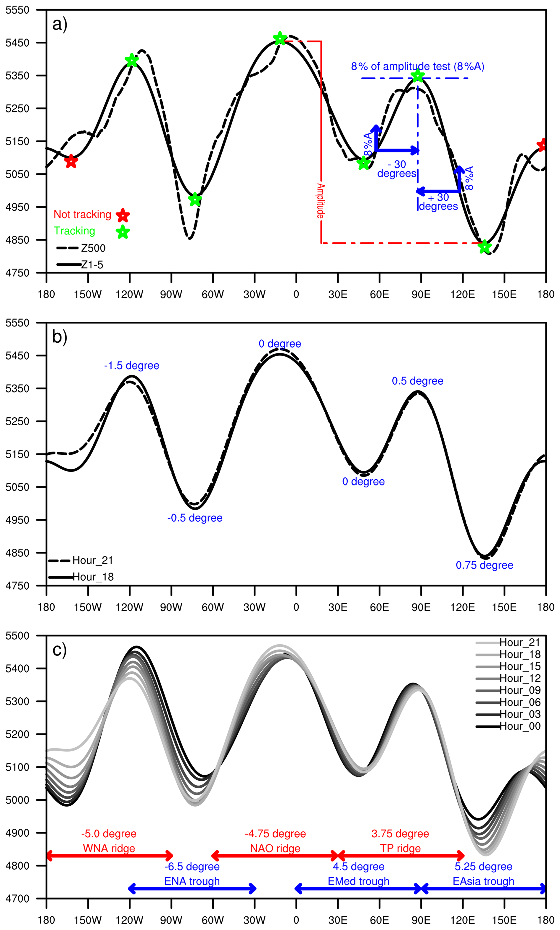
Figure 3 (a) The 500 hPa geopotential height field (Z500; dashed, black line) and the sum of the first five zonal Fourier-decomposed waves of Z500 (Z1–5; solid, black line) for 7 January 2003, at 60° N. The blue text and arrows are associated with a threshold metric that identifies the strength of the ridges and troughs (see method for more information). Based on this threshold, three ridges and three troughs (green stars) are high and deep enough, respectively, to be detected by the tracking algorithm. In this time step, the tracking algorithm will ignore one ridge and one trough (red stars) that do not meet this threshold. (b) The Z1–5 for two consecutive time steps (3 h) and the changes in the ridges' and troughs' longitudinal location between these time steps (positive eastward). (c) The Z1–5 for 1 d (8 time steps) and the calculated longitudinal shifts of each ridge and trough over the entire day.

We estimate the speed of atmospheric wave zonal propagation by utilizing a ridge and trough tracking algorithm (Fig. 3a). Small amplitude ridges and troughs are ignored since they are often short lived (red stars in Fig. 3a). This is accomplished by considering a threshold for the gph at each local maximum (ridge) and local minimum (trough): at each time step (3-hourly) and latitude, the gph at the ridge (trough) position must be greater (less) than the gph at 30° to the west and east of the ridge (trough) position by at least 8 % of the Z1–5 amplitude (see blue texts and arrows in Fig. 3a). The Z1–5 amplitude is defined as the difference between the highest ridge and the lowest trough at all longitudes around a latitude circle at each time step and latitude. These criteria were carefully chosen after multiple experiments to ensure that all large waves are tracked while minor waves are neglected. Nonetheless, in all the experiments, as long as the thresholds do not suppress large waves, the drawn overall conclusions regarding wave speed changes remain unchanged for other parameter settings. We track each local ridge and trough in time over longitudes to find the ridge and trough speed, respectively. Also, we save all local ridge latitude and longitude (RLL) and trough (TLL) positions. At each latitude, ridges and troughs are labeled according to their positions (longitude) and are tracked to the next time step by searching for the nearest ridge or trough within a 12° limit both to the west and east of their location (Fig. 3b). If no corresponding feature is detected within this range, the ridge or trough is considered to have decayed. Conversely, if a new ridge or trough appears without a corresponding feature in the previous time step, it is considered to have formed.

Figure 4 displays the probability of the winter climatological positions of ridges and troughs, as well as the decay and formation of these features. Throughout winter, ridges and troughs tend to appear with greater frequency in certain areas compared to others (Figs. 4 and S4). This study focuses on three primary locations for ridges and three for troughs, assigning specific names to the ridges and troughs that occur in these regions. The three main ridges are located over the west coast of North America (hereafter, WNA ridge), the western flank of the Tibetan Plateau (hereafter, TP ridge), and the North Atlantic Ocean (hereafter, NaO ridge, at low latitude over the middle part and at high latitude over the eastern part of the ocean). The three main troughs are located over Eastern North America (hereafter, ENA trough), the eastern Mediterranean (hereafter, EMed trough), and East Asia (hereafter, EAsia trough). The daily speed of these six major ridges and troughs is determined by summing their 3-hourly values across their respective longitudinal ranges (Fig. 3c). The speeds of the ridges over 180–90° W, 60° W–30° E, and 30–120° E are added to calculate the daily speeds of the WNA ridge, the NaO ridge, and the TP ridge, respectively. The daily speeds of the ENA trough, EMed trough, and EAsia trough are also found by taking the sum of the speeds of the troughs over 120–30° W, 0–90° E, and 90–180° E, respectively (Fig. 3c).

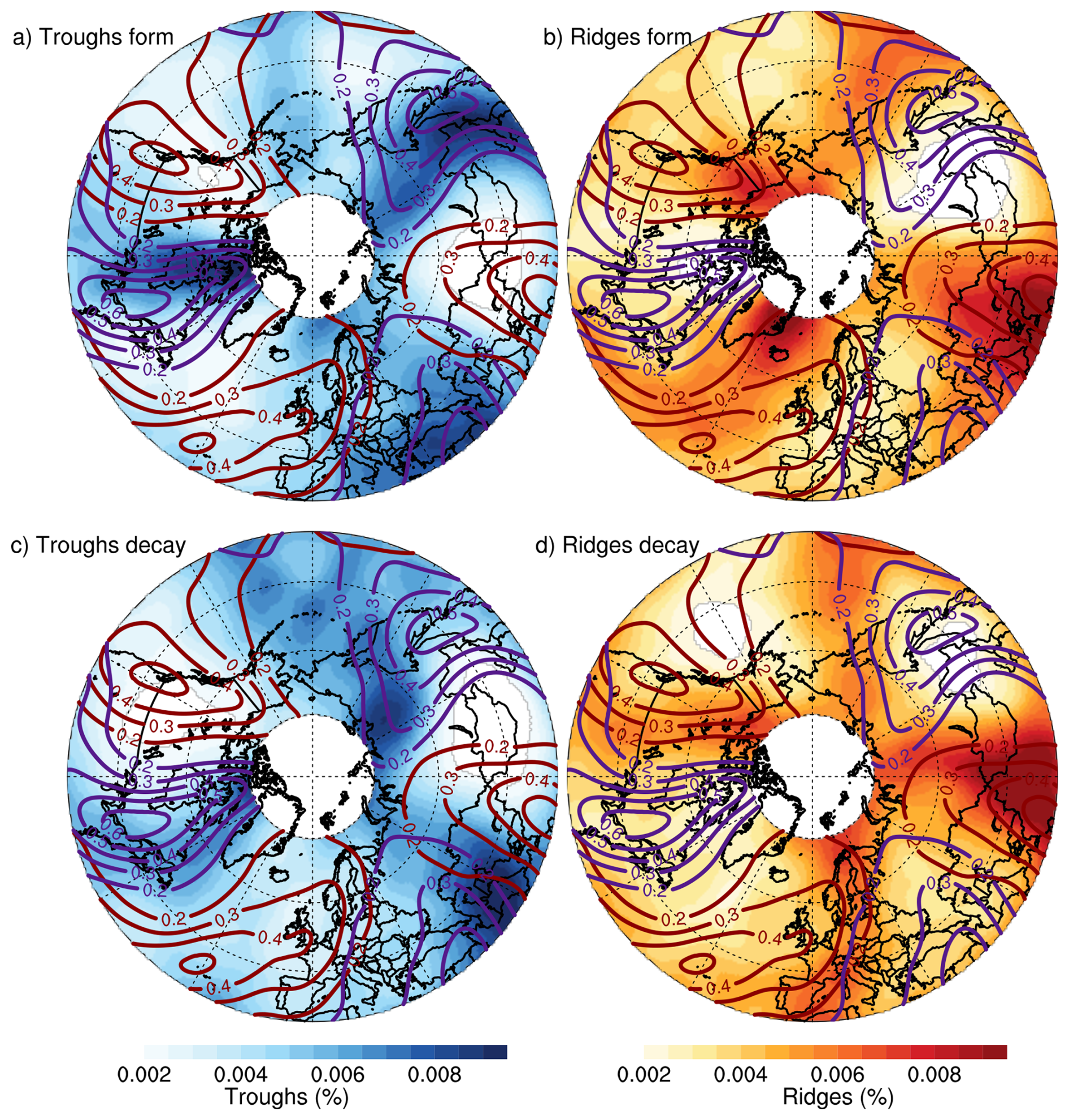
Figure 4 The probability of ridges and troughs and their formation and decay as a function of location. Shown with contours are the probabilities (in percentage) of 300 hPa ridges (brown) and troughs (purple) during winter climatology as a function of location. The blue shading indicates the climatological probability of (a) formation and (c) decay of troughs as a function of location. The red shading indicates the climatological probability of (b) formation and (d) decay of ridges as a function of location. A Gaussian function, using a weighted running average over eight degrees in latitude and over an equal distance in longitude, is used to smooth the probabilities.

Ridges and troughs typically form upstream of their climatological positions, sometimes wobble around these locations for several time steps (or days), and subsequently decay downstream (Fig. 4). The WNA ridge, NaO ridge, and ENA trough exhibit stronger formation and decay at high latitudes compared to mid-latitudes, indicating that these ridges and troughs tend to persist longer in the midlatitudes. The TP ridge and EMed trough show large formation and decay at mid-latitudes, likely due to their interaction with the complex orography. Nonetheless, the likelihood of their decay and formation remains significantly lower than their climatological existence, indicating persistency of the ridges and troughs (Fig. 4). The EAsia trough forms more strongly at midlatitudes, while its decay is more pronounced at higher latitudes. Over the Pacific Ocean, there is one ridge and one trough formation center, both of which decay downstream from their formation center. As can be seen from the climatological position of ridges and troughs, there is no strong ridge or trough in these locations, suggesting that these features are short-lived.

The probabilities of climatological ridge and trough positions here differ significantly from those in Schemm et al. (2020), mainly due to differing detection methods. Schemm et al. (2020) identify ridges and troughs by comparing nearby grid points, while our method compares values across all longitudes at each latitude. Consequently, their probabilities are higher at high latitudes, where ridges and troughs are more distinct, but lower at low latitudes due to local gph flattening. Our method, however, still indicates ridges and troughs at subtropical and tropical latitudes, but these could rather be assigned to patterns such as subtropical highs than Rossby waves. Additionally, the probabilities estimated by our method represent the likelihood of ridges or troughs occurring at a specific location, rather than over an area defined by exceeding a curvature threshold of the gph field as in Schemm et al. (2020); hence, the probabilities in our study are naturally much lower than those reported by Schemm et al. (2020).

3.2 Trough and ridge amplitude

Several metrics have been developed to study the waviness of the atmosphere (e.g., Francis and Vavrus, 2012; Barnes, 2013; Hassanzadeh et al., 2014; Chen et al., 2015; Cattiaux et al., 2016; Geen et al., 2023), many of which rely on the meandering of the 500 hPa isohypses (lines of constant gph) as a proxy. Considering the variations of wave amplitude with different isohypses – e.g., associated with the seasonal variability and poleward shift due to global warming (Barnes, 2013) – selecting an appropriate isohypses is critical. To address these challenges, Cattiaux et al. (2016) derived isohypses from the daily average of the gph at 500 hPa between 30 and 70° N, hereby varying in time. They regarded the meandering of these isohypses as an indicator of the waviness of the atmospheric flow at 50° N.

Here we focus on identifying changes in waviness at each latitude and at 300, 500, and 850 hPa, which requires some modification of the Cattiaux et al. (2016) approach: For a given study region, the most common isohypse at each time step and latitude is taken as the zonal average of the gph over half of the hemisphere centered on the center longitude of each study region. Then, the meridional wave extent for that latitude is defined as the meridional extent of the associated isohypse determined by calculating the difference between the maximum latitudinal location and the minimum location of that isohypse (total gph isohypse extent; TIE). By focusing on half of the hemisphere, it is ensured that at least one full ridge and trough are included within the region. In a similar way, the meridional extent of the first five Fourier decomposition wave numbers of gph (Z1–5) is calculated (planetary isohypse extent; PIE). During cold spells in the defined regions, both TIE and PIE demonstrate the same significant pattern of changes (not shown). This shows the modest impact of small waves on the wave amplitude changes during cold spells. Therefore, we only consider the results of the meridional extent of Z1–5.

Some isohypses have unconnected subparts (see Fig. 5a), referred to as cut-off low and cut-off high, which might lead to interpretation errors in the wave amplitude. For instance, in Fig. 5a, at high latitudes (around 85° N), the most common isohypse is 8300 m, and at these latitudes, the waviness of this isohypse is small. But, due to a cut-off low of this isohypse at midlatitudes, the estimated wave amplitude at 85° N is large. Moreover, the PIE does not specify the separate contribution to the wave amplitude from ridges and troughs. Understanding these contributions is critical, especially during cold spells, as it helps determine which parts of the wave – ridge or trough – have the greater impact.

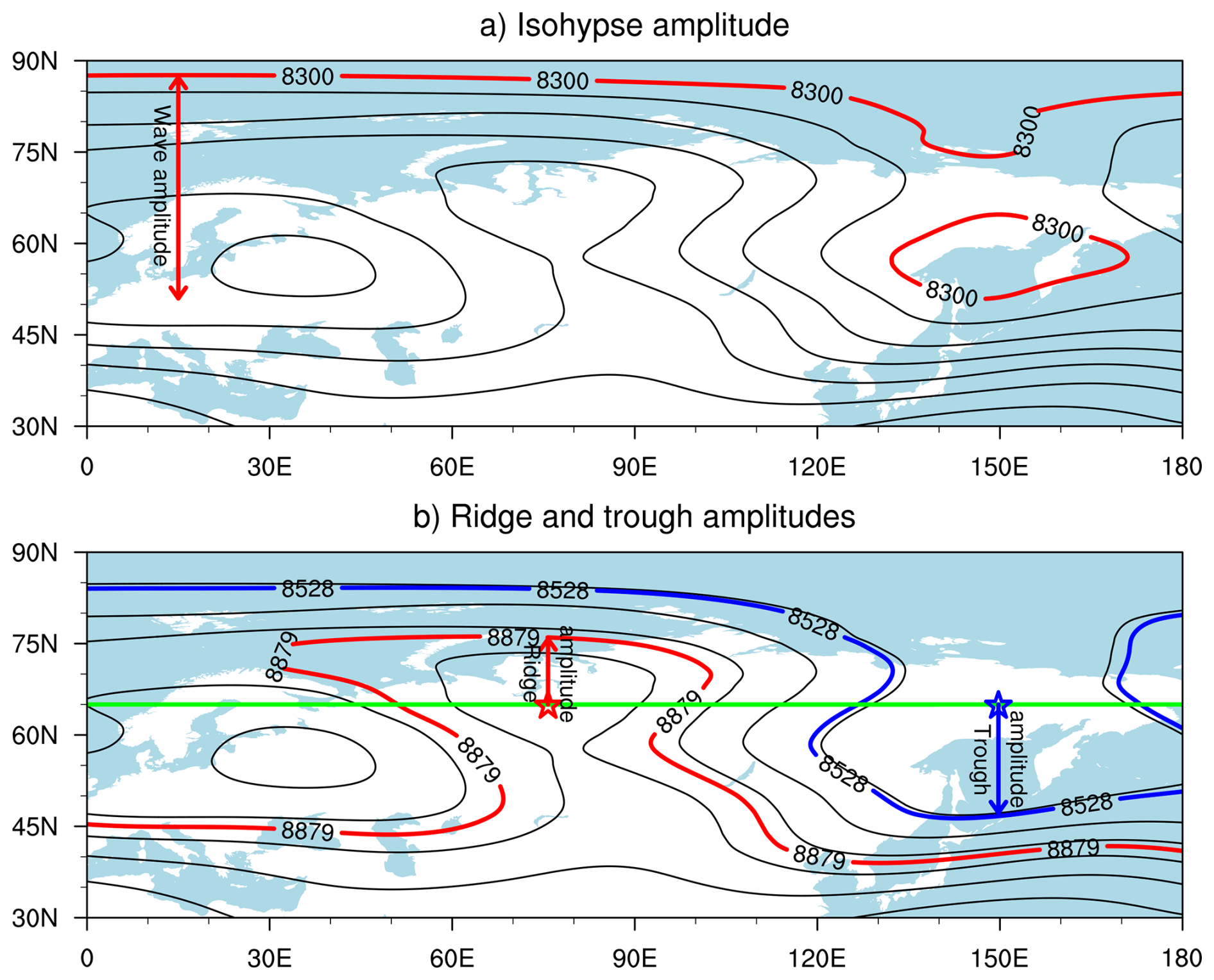
Figure 5 The sum of the first five zonal Fourier-decomposed waves of the 300 hPa geopotential height field (Z1–5) for 4 January 2016, at 18:00 UTC. (a) The 8300 isohypse and its amplitude are highlighted; (b) the ridge (red arrow) and trough (blue arrow) meridional amplitudes at the ridge (red star) and trough (blue star) center at latitude 65° N (green line). The 8879 isohypse (red line) and the 8528 isohypse (blue line) are determined by the zonal average of the Z1–5 over a 90° longitude range centered at the ridge and trough positions, respectively, at 65° N.

Hence, we here propose an alternative metric where the meridional extent of the Z1–5 ridges and troughs are measured separately (Fig. 5b). The meridional extent of the ridge is given as the latitudinal difference between the RLL and the isohypse determined by the zonal average of the Z1–5 over a 90° longitude range centered at the RLL (Fig. 5b, red line); hence, the meridional extent of a ridge at a given latitude is obtained as the difference between that latitude and the latitude of the first cross of the isohypse when moving northward along the longitude of the RLL. The employed method does not take into account the possible meridional tilting of waves. To address this, at 300 hPa, the wave amplitude is calculated for all longitudes within the 90° longitude range. The highest value obtained is then considered the meridional amplitude of the ridge. While the highest value often yields slightly larger wave amplitudes than that obtained at the RLL, the overall conclusions regarding changes in wave amplitude during cold spells remain the same for both approaches (not shown). Therefore, to reduce computational usage, we used the amplitude at the ridge position. The meridional extent of troughs is obtained in a similar way but moving southward from TLL.

The estimated meridional amplitudes of a given ridge (trough) are highly influenced by the longitudinal range over which the zonal average of the Z1–5 is taken for determining the isohypse. Using a smaller longitude range yields an isohypse value closer to the value of Z1–5 at RLL (TLL), which leads to small amplitudes. Using a large longitude range might yield an isohypse that cannot be found near the RLL (TLL), resulting in a missing value for the amplitude. Therefore, after conducting multiple experiments, the 90° threshold is chosen. Nonetheless, despite the arbitrariness of the meridional wave amplitude when defined this way, its magnitude exhibits a consistent latitude-dependent pattern and comparable bands of significance in both the climatology and cold-spell cases, which is important and sufficient for this study.

To compare the results of the refined method with PIE, considering the total wave amplitude, the average of the amplitude of the ridges plus those of the troughs over half of the hemisphere centered at each study region is calculated (ridge-trough isohypse extent; RTIE). For climatology, the RTIE amplitude (Fig. S2, gold lines) is nearly half of the PIE amplitude. During cold spells, there are likewise many similarities between the RTIE and the PIE, yet they have some important differences. During cold spells, the PIE amplifies over a wider latitude range compared to the RTIE. This could be attributed to the influence of cut-off lows or cut-off highs on the amplitude of distant locations.

4 Application of the wave metric to cold spells

4.1 Wave location

To investigate the impact of atmospheric waves on the formation of winter cold spells, nine regions with a high likelihood of cold spells are selected (Fig. 2). These regions are chosen based on their significant contribution to the historical extreme 2 m temperature days on a hemispheric scale (see Sect. 2.2). During cold spells over North America (R01, R02, and R03), large-scale gph anomaly patterns show an anticyclonic gph anomaly over the North Pacific and a cyclonic gph anomaly over North America (Fig. S3a, b, and c), similar to the findings of other studies (e.g., Xie et al., 2017). During cold spells, the WNA ridge and the ENA trough are located to the west of their corresponding climatological positions (Fig. 6a, b, and c). This repositioning is more pronounced for R02 and R03 than for R01. The NaO ridge extends from northwest Africa to northwest Europe, specifically exhibiting an eastward relocation at lower latitudes. For cold spells over western regions of Europe (R04, R05, and R06), the gph anomaly at 500 hPa shows a positive anomaly located north of a negative anomaly (Fig. S3d, e, and f). This anomaly resembles a high-over-low North Atlantic blocking situation, which is similar to the findings of other studies (e.g., Trigo et al., 2004; Buehler et al., 2011; Pfahl, 2014). For R04 and R05, at high latitudes, the locations of the NaO ridge and EMed trough tend to be to the west of their respective climatological centers (Fig. 6d and e). During cold spells over Eastern Europe (R08), the EMed trough and the TP ridge at high latitudes are located to the east of their respective climatological locations (Fig. 6h). The cold spell over Northern Siberia (R09) primarily aligns with a deep trough downstream over northwest Asia, as depicted in Figs. S3i and 6i. Despite the high latitude of this region, it is sufficiently far from the pole to be affected by cold advection from higher latitudes during cold spells (Tuel and Martius, 2024). For R09 (Fig. 6i), ridges form over the western flank of the Ural Mountains, and the EAsia trough at high latitudes is located in the west of its climatological location. These findings indicate that a distinct positioning pattern of ridges and troughs on a hemispheric scale occurs during cold spells over each region. These patterns can also be observed at 500 hPa (not shown) and 850 hPa (not shown), indicating that during cold spells the entire troposphere is located in a rather barotropic manner. These findings suggest an interaction between atmospheric dynamics and surface temperatures.

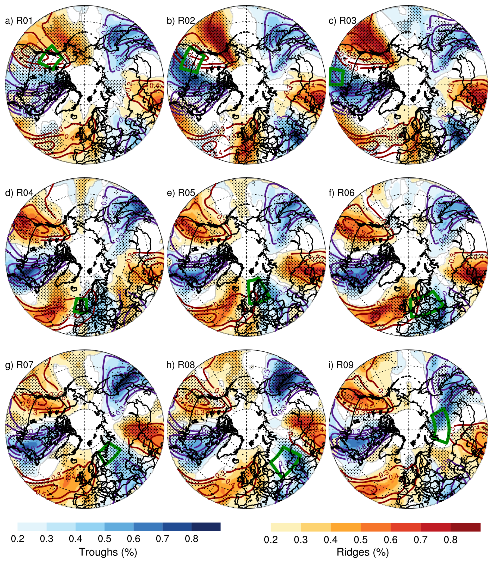
Figure 6 The probability of ridges and troughs at 300 hPa as a function of latitude and longitude. The shading (based on all-time steps of the cold spells) and contours (climatology) indicate probabilities of ridges and troughs in percentage. Solid brown (purple) contours represent the climatological probability of ridges (troughs). Red (blue) shading represents the probability of ridges (troughs) during cold spells over each region. As the probabilities of ridges and troughs are computed individually, shading and contours of the two fields are shown for values greater than 0.2 % to minimize overlap in the plot. Dots indicate regions where cold spells and climatology are significantly different at the 95 % confidence level. The green box in each plot shows the location of cold spells. A Gaussian function, using a weighted running average over eight degrees in latitude and over an equal distance in longitude, is used to smooth the probabilities. (a) Northwest Canada; (b) Northwest US and Southwest Canada; (c) Central US; (d) British Isles; (e) Scandinavia; (f) Europe; (g) Northwest Russia; (h) Southwest Russia; and (i) Northern Siberia.

Figure 7 shows the time-development of ridges and troughs before and during cold spells for the composites of regions in North America and Europe. This choice is based on the similarity of the upstream ridge and downstream trough in the selected regions for each composite. In North America, cold spell regions are predominantly located in the vicinity of the WNA ridge. In North America, before cold spells occur, the ridge encompasses a broad area, including the cold-spell regions (Fig. 7a). At the start of cold spells, the upstream ridge becomes more localized in the western side of the cold-spell regions (Fig. 7e). This pattern provides northerly wind flow from the Arctic toward the cold-spell area (Fig. S4). In Europe, most of the cold spell regions are primarily located in the vicinity of the EMed trough. Similar to North America, before cold spells occur, the ridge encompasses a wide area (Fig. 7b), indicating that cold or warm anomalies are not concentrated to specific locations. However, with the onset of cold spells (Fig. 7f), ridges and troughs become more concentrated, with a ridge positioned upstream and a trough located within the cold-spell regions (Fig. 7f). Hence, associated with cold spells, roughly the same type of regional-scale circulation pattern is found in both North America and Europe. These findings highlight the critical role of the nearest upstream ridge and downstream trough in the formation of cold spells.

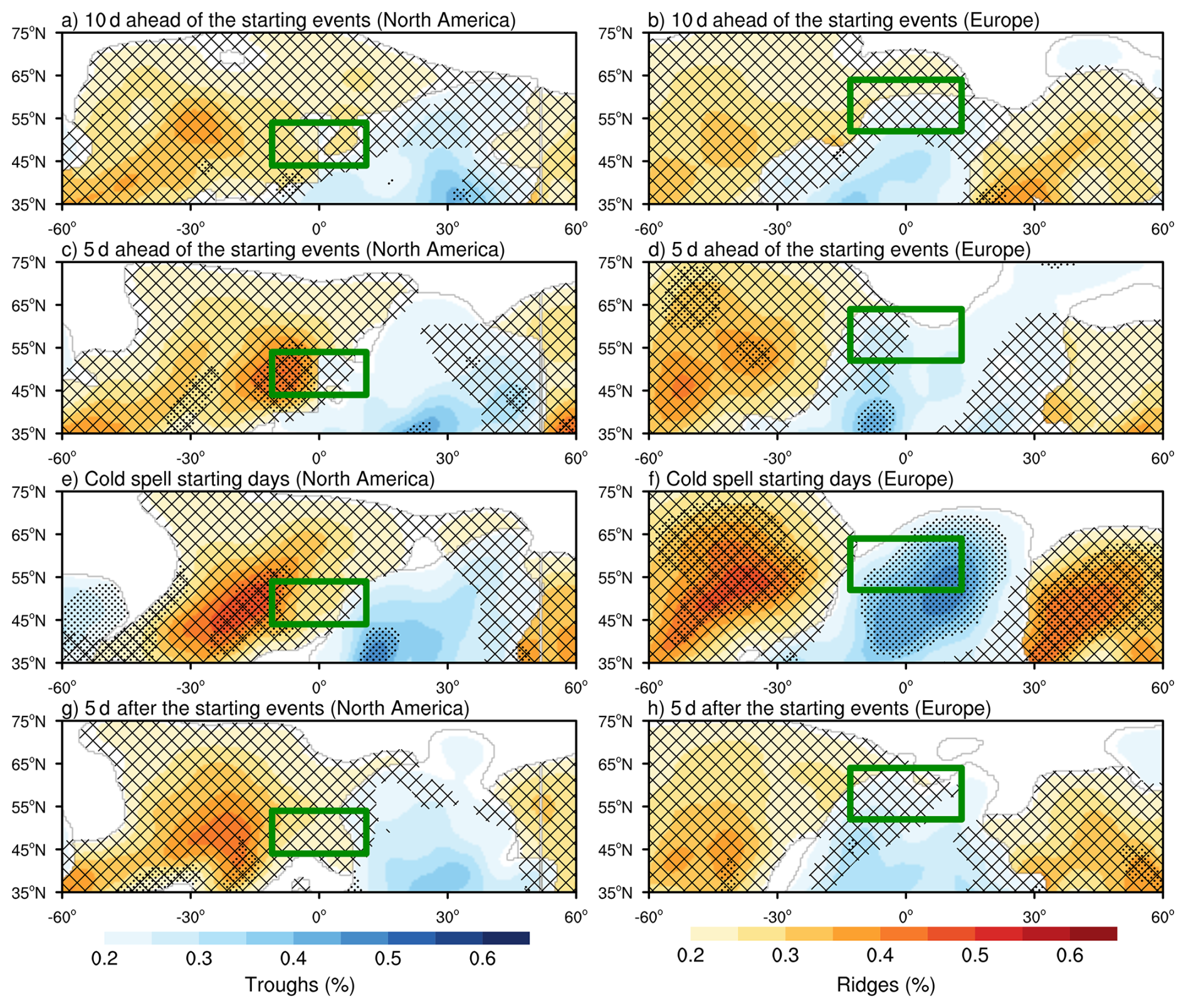
Figure 7 The probability of ridges and troughs at 300 hPa as a function of location and time relative to the start of the cold-spell events. Shown with shading are probabilities (in percentage) of ridges (red) and troughs (blue) for different time lags averaged over all cold spells in the study regions relative to the center of the cold-spell region. The panels on the left correspond to the composite of cold spells in North America (R01, R02, and R03), and the panels on the right correspond to the composite of cold spells in Europe (R04, R05, R06, R07, and R08). To show both ridges and troughs in a single plot, priority is given to the stronger feature. The hatched areas represent grid points where ridges are occurring, and dots indicate regions where ridges and troughs during cold spells are significantly different from the climatology at the 95 % confidence level. The green box shows the average latitude and longitude span of the cold spell regions. A Gaussian function, using a weighted running average over eight degrees in latitude and over an equal distance in longitude, is used to smooth the probabilities. (a, b) 10 d ahead of the starting cold spells; (c, d) 5 d ahead of the starting cold spells; (e, f) cold spell starting days; and (g, h) 5 d after the start of cold spells.

4.2 Trough and ridge amplitude and speed

For cold spells, the largest ridge and trough amplitude and speed differences relative to climatology occur for the local upstream ridge and downstream trough (Figs. S5 and S6). Generally, the amplitude and speed differences of ridges and troughs decay as their distance increases from the location of the cold spell. A composite over all cold spells and regions of the upstream ridges and downstream troughs provides a general overview of the local wave behavior during cold spells (Fig. 8). The following refers to changes in ridges or troughs (such as amplification or slowing down), indicating significant alterations in their behavior during cold spells compared to the climatological average behavior of these features within their respective longitude bands. The upstream ridge significantly amplifies (Figs. 8a and S5), facilitating the transfer of Arctic cold air to the cold spell region. During cold spells, the northward winds entering the Arctic are increasing west of the upstream ridge, while the southward winds exiting the Arctic are increasing east of the upstream ridge (Fig. S4). The upstream ridge also significantly slows down (Figs. 8b and S6), implying an increase in the persistence of the warm northward wind to the Arctic and the cold southward wind to the cold spell location. The persistent warm northward wind to the Arctic might be the reason behind the correlation between cold events and a warmer Arctic found in other studies (e.g., Cohen et al., 2018); yet more research is needed to discover the impact of the amplified ridge on Arctic temperatures. At low latitudes, the upstream ridge moves faster during cold spells, which are mainly associated with North America and northern Siberia (Fig. S6). The underlying reasons for this pattern are not clear and are left for future research.

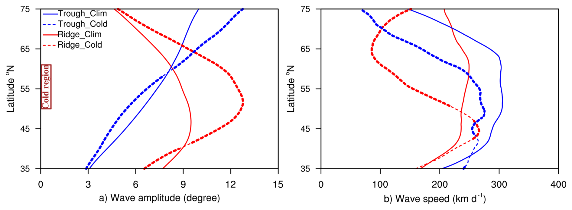
Figure 8 Climatology (solid lines) and composite of cold spells over all study regions (dashed lines) for (a) wave amplitude (°) and (b) wave speed (km d⁻¹) at 300 hPa. Red and blue lines are showing the average of the upstream ridge and the downstream trough, respectively, in the vicinity of each cold spell region. Bold dashed lines indicate a significant difference between the cold spell and climatology at the 95 % confidence level. The brown box on the left side shows the average latitude span of all cold spell regions. A 4° running average is applied to smooth the lines.

The downstream trough amplifies (deepens) at latitudes north of the cold spell location, while it weakens at southerly latitudes (Figs. 8a and S5). For the cold-spell regions in the southern as compared to the northern mid-latitudes, the increase in trough amplitude develops more to the south (Fig. S5). Amplification of this trough contributes to enhancing the southward cold wind from the Arctic into the cold spell region (Fig. S4). Similar to the upstream ridge, the downstream trough significantly slows down (Figs. 8b and S6), hereby increasing the persistency of the cold southward winds into the cold spell region.

4.3 Lead-lag analysis

In the previous section, it was shown that cold spells are associated with higher-amplitude and slowing ridges and troughs in the vicinity of the cold spells. This raises the question of the timing of these changes in relation to the occurrence of cold spells. Previous research has shown that upper-atmospheric changes – such as amplified planetary waves (Screen and Simmonds, 2014), blocking (Kautz et al., 2022), and the stratospheric polar vortex (Tomassini et al., 2012) – can lead to surface extreme events. Here, a day-lag analysis of composites over cold spells is provided to shed light on the causal relationship between upper-level waves and surface temperature (Figs. 9 and S7). Since the largest wave amplitude and speed differences relative to climatology belong to the upstream ridge and the downstream trough, their time series are plotted here.

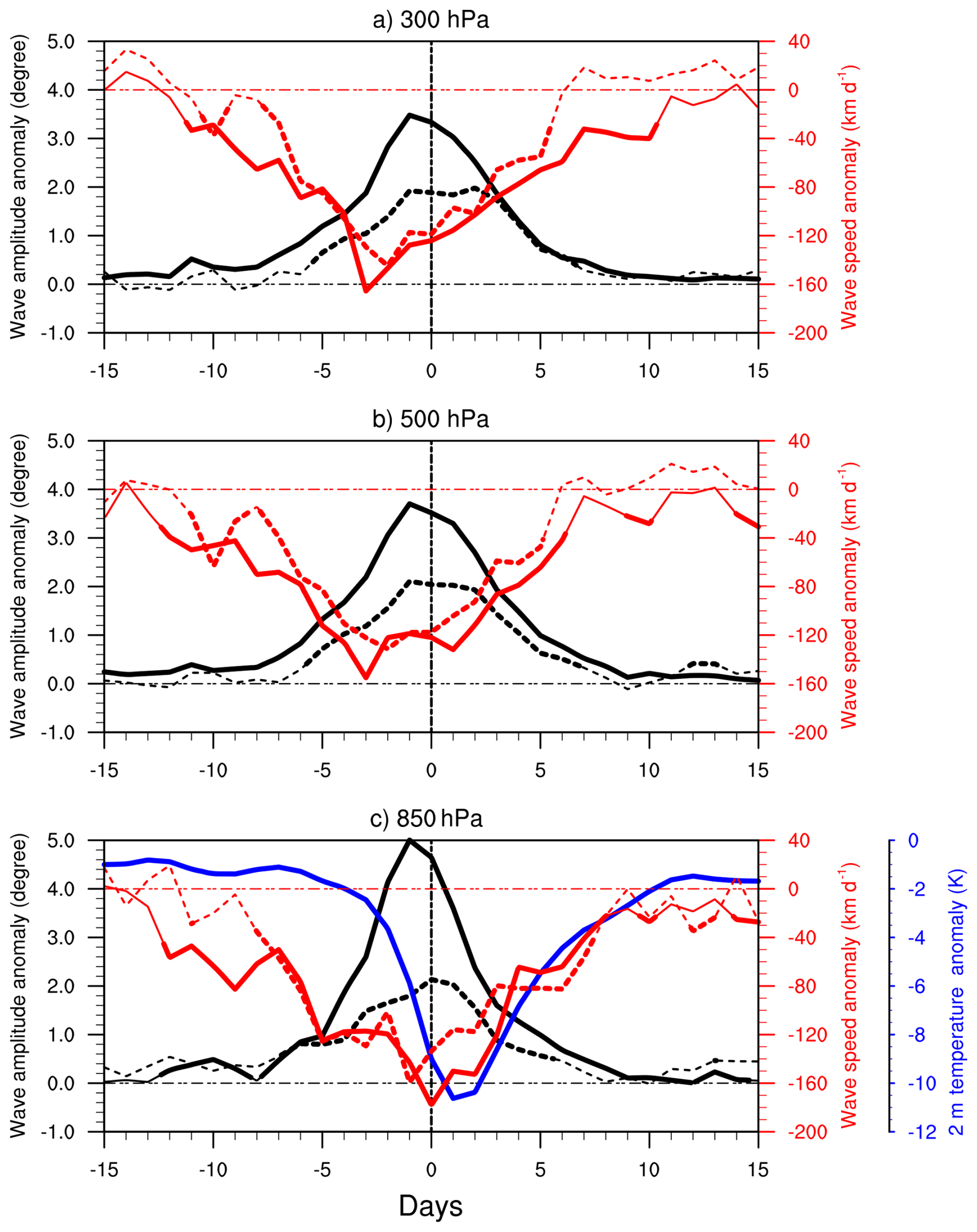
Figure 9 Composites of anomalies relative to climatology of 2 m temperature, and ridge and trough speed and amplitude during all cold spells as a function of time lag for all study regions. The lag zero (zero on the x axis) is the day that 30 % of the land in a given region experiences a cold spell. Blue line is the composite of temperature anomalies averaged over the whole study region. Black and red lines are the composites of ridge and trough amplitude and speed anomalies, respectively. The upstream ridge and the downstream trough in the vicinity of the cold-spell location are shown by solid and dashed lines, respectively. The latitude bands with a significant positive wave amplitude anomaly and a negative wave speed anomaly are averaged for each cold spell region (indicated by the vertical solid lines on the right-hand side of Figs. S5 and S6). Bolded solid and bolded dashed lines indicate the difference to climatology significant on a 95 % level. Shown are patterns of (a) 300 hPa, (b) 500 hPa, and (c) 850 hPa.

The minimum speeds of the upstream ridge and downstream trough occur at a negative time lag several days prior to the onset of the cold spell, which is taken as 30 % of grid points in the region experiencing a cold spell and indicated by the lag zero. Both amplified ridge and trough are also encountered prior to the cold spell, but the speed reduction precedes the amplitude increase (Fig. 9a and b). This could potentially be attributed to the breaking of waves associated with exceeding the wave for the wave activity flux (Nakamura and Huang, 2018). In addition, this pattern can also be explained by the poleward excursion of low-potential vorticity subtropical air ahead of a slowly moving elongated trough (Hoskins et al., 1985). The preceding of the upstream ridge and the downstream trough amplification relative to the cold spell suggests that cold spells arise as a result of slow and amplified local upper-atmospheric waves. For Northern Siberia, the downstream trough amplifies at a positive time lag several days after the cold spells (Fig. S7i), indicating that the amplified trough cannot be responsible for the cold spell in this region. This is consistent with the formation of cold spells in Northern Siberia being due to diabatic processes (Röthlisberger and Papritz, 2023). Nonetheless, the upstream ridge amplifies and slows down prior to the onset of cold spells in this region (Fig. S7i). The wave speed anomaly shows almost the same pattern for both 500 and 300 hPa (Fig. 9a and b), which suggests an almost barotropic wave signal through the troposphere during cold spell events. However, the wave-speed reduction occurs somewhat later at 850 hPa, indicating a downward propagation of the wave-speed signal.

The lead-lag behavior of other significant and non-significant changes in the upstream ridge and downstream trough (Figs. S5 and S6) is also analyzed. Their time lag either shows no significant changes or occurs after the upstream ridge and downstream trough's significantly positive amplitude and negative speed anomalies (not shown). However, there are some exceptions: During cold spells over North America (R01, R02, and R03), the lead-lag behavior of the upstream ridge anomaly at the lower midlatitudes (35–50° N) indicates that this ridge slows down at these latitudes before it does at other latitudes (Fig. S8a). For both Eastern European regions (R07 and R08), latitudes with a reduction in the upstream ridge amplitude (35–40° N; Fig. S7g and h) show strong negative amplitude anomalies weeks before the onset of the cold spell (Fig. S8b). This indicates that the ridge at lower latitudes tends to move zonally, which may weaken the mixing of warm tropical air with colder midlatitude air long in advance of the cold spell formation.

5 Conclusions

The present study provides a comprehensive perspective on the formation of cold spells in the midlatitudes, demonstrating that increased wave amplitude and decreased speed are fundamental drivers of cold-spell development. Here, the focus is on the role of large-scale Rossby waves in these cold spells. We utilized a novel ridge/trough tracking method that identifies large-scale ridges and troughs derived from the first five zonal Fourier decompositions of the gph field. Because our detection targets the large-scale (Z1–5) components, it primarily captures the slow wobbling of climatologically preferred ridges and troughs and may under-detect weaker, transient synoptic features, particularly at lower latitudes.

Across all midlatitude regions, locally amplified and slowing ridges and troughs near cold spells appear important for the formation of these. Through a daily lag analysis, a cause-and-effect relationship between upper-level waves and extreme cold surface temperatures is revealed, indicating that upper-level waves are preceding cold spells and hence important for the development of these. Our findings support previous research conducted in a specific region, indicating that slow (e.g., Fragkoulidis and Wirth, 2020) and amplified (e.g., Jolly et al., 2021; Fragkoulidis and Wirth, 2020) Rossby waves contribute to cold spells in Europe. Moreover, we demonstrate the importance of ridge and trough development at each latitude within the mid-latitudes, whereas others (e.g., Fragkoulidis and Wirth, 2020) discuss daily averages of speed and amplitude over an area encompassing the cold-spell region. By focusing on latitude rather than averaging over a broader region, we determine that the slow and amplified waves are mostly in the vicinity or north of the cold spell regions.

Additionally, we discuss the importance of wave location in cold spell development, as different configurations of ridges and troughs, compared to their typical winter climatological positions, can result in a cold air advection from the north to the cold-spell region. Our findings highlight the critical importance of large-scale wave location (Z1–5), emphasizing the need to consider potential shifts in these wave positions in a warming world. Such shifts could result in more frequent extreme events in certain areas, impacting local climates.

It is important to note that this research primarily focuses on the nearest ridge and trough relative to the location of cold spells. However, an upper-level anomaly can propagate both downstream and upstream (e.g., Simmons and Hoskins, 1979). Consequently, the anomaly that ultimately triggers the formation of cold spells may initially originate from a remote ridge or trough, and further investigation is required to explore each region in greater depth.

Considering the increasing frequency of heat waves, floods, and droughts due to climate change (IPCC; Seneviratne et al., 2021), there is a need to understand their dynamical drivers (Xu et al., 2024). In this context, we have developed two tools designed to identify the amplitude and speed of large-scale atmospheric waves, which can be utilized in future research to unravel the dynamical drivers of various types of extreme events. Furthermore, these metrics may help clarify the impact of Arctic amplification on the waviness and speed of Rossby waves. Our meridional wave amplitude metric provides a unique methodology compared to other metrics (Geen et al., 2023), as it could evaluate changes in ridge and trough independently in a warming world.