Quantifying the tropospheric response to individual sudden stratospheric warmings revealed by an ensemble simulation strategy

Stratospheric extreme events during Northern winter and spring have been shown to sometimes enhance the sub-seasonal predictability of large-scale tropospheric circulation patterns such as the North Atlantic oscillation (NAO) and Greenland/European blocking. However, it remains unclear whether event-to-event differences in the observed tropospheric evolution after individual sudden stratospheric warmings (SSWs) represent a robust difference in the tropospheric response to the events, or whether such differences in tropospheric evolutions are simply caused by tropospheric variability. To make progress on this question, we robustly quantify the tropospheric response with an ensemble simulation strategy in a controlled model environment. We construct a model climatology using the ICON global numerical weather prediction (NWP) model, representing a wide range of realistic stratosphere–troposphere evolutions during winter months, but under controlled boundary conditions to exclude confounding factors like teleconnections of tropical origin. The simulations reproduce key aspects of observed stratosphere-troposphere coupling, providing a consistent framework to assess event-specific tropospheric responses. We produce spin-off ensembles for selected SSW events; the corresponding ensemble means help robustly quantify the tropospheric response to these SSWs. We find pronounced and robust event-to-event differences in the tropospheric response to SSWs. We further show that the flow anomalies in the lower stratosphere during the second week are well correlated with the surface response 3–7 weeks after the SSW. Moreover, our results indicate that the formation of wave reflection surfaces within the lower stratosphere may prevent the establishment of persistent lower-stratospheric anomalies. Overall, our controlled model simulations show that individual SSWs may differ significantly in their likelihood to induce a tropospheric response and that this likelihood is mainly determined by the post-SSW flow evolution within the stratosphere. These results may be relevant for sub-seasonal predictability of surface weather, especially given that the stratospheric part of the response to SSWs is highly predictable.

1 Introduction

Sudden stratospheric warmings (SSWs) are a prominent feature of the Earth's atmospheric dynamics and are known to have a significant impact on tropospheric weather. These changes in the tropospheric circulation are typically (i.e., on average over many SSWs) characterised by negative anomalies in the North Atlantic Oscillation (NAO) and Arctic Oscillation (AO), resulting in an equatorward shift of the jet stream and storm tracks in the Northern Hemisphere (further details in Domeisen et al., 2020a). Stratospheric and tropospheric dynamics mostly evolve on substantially different timescales, the former typically within weeks, and the latter typically within several days. This separation of timescales implies that stratospheric anomalies associated with SSWs can introduce a degree of persistence into the coupled system, such that the correlation between tropospheric and stratospheric variability is particularly important for forecasts running longer than 2 weeks (sub-seasonal and longer). Accurately simulating the fundamental principles governing troposphere-stratosphere interactions can enhance the accuracy of sub-seasonal forecasts, as well as extend the corresponding time ranges of predictability.

Despite the well-documented average influence of SSWs on tropospheric circulation patterns (see e.g., Baldwin and Dunkerton, 2001), attributing a given tropospheric post-SSW evolution to an individual SSW is not straightforward. This is because any stratospherically induced response is small compared to internal tropospheric variability (see e.g., Oehrlein et al., 2021). As a consequence, a given single-event post-SSW anomaly near the surface, even if it strongly resembles the canonical SSW response (e.g., obtained from composite means) does not by itself demonstrate a genuine downward coupling response – the troposphere may have fortuitously produced such a canonical response-like signal independently of the stratospheric evolution (more akin to an apparent response), as shown in e.g., Davis et al. (2022). Likewise, the lack of a single-event post-SSW canonical surface anomaly does not by itself demonstrate a lack of downward coupling – in this case, the full tropospheric evolution may have overwhelmed the (small) actual SSW response (see e.g., Domeisen et al., 2020b). In other words, for individual observed SSWs one cannot distinguish apparent from genuine surface responses to SSWs (or a lack thereof). As we argue below, ensemble simulations offer a powerful tool to attribute anomalous surface signatures to SSWs.

One powerful approach to attribute anomalous post-SSW surface signatures to that SSW for single events is based on ensemble simulations. Specifically, the ensemble mean for sufficiently large ensembles offers a possibility to average out intrinsic tropospheric variability, thereby providing a proxy for the SSW-induced surface response. By effectively isolating the mean signal, this approach may be applied to multiple individual SSWs, which then also allows one to determine whether the magnitude and structure of the responses vary substantially between individual stratospheric events. Such an ensemble-based approach has previously been applied to characterise the response to SSWs (see e.g., Kautz et al., 2020; Hitchcock and Simpson, 2014). A more recent and comprehensive application is provided by the SNAPSI project, within which ensemble re-forecasts were conducted by multiple model centres, initialised around three different observed SSWs (two in the Northern, one in the Southern Hemisphere) to assess their contribution to surface predictability on sub-seasonal timescales (Hitchcock et al., 2022). Using these ensemble re-forecasts, it was demonstrated that averaging across forecast members enables the isolation of a robust tropospheric signal following SSWs (see e.g., Dai et al., 2025; Hitchcock et al., 2022). The sub-seasonal-to-seasonal (S2S) database also offers the possibility of studying the tropospheric response to observed SSWs with ensemble simulations from multiple modelling centres (see e.g., Karpechko et al., 2018; Rao et al., 2020, 2021; Butler et al., 2020). In a more recent study, Nebel et al. (2024) analysed the tropospheric response to 16 observed SSWs in S2S ensemble re-forecasts and found a varying mid-tropospheric response between events.

However, these approaches are constrained by the limited number of observed SSWs for which sufficiently large ensemble simulations are available (in some cases requiring the combination of ensembles from different forecasting models, which introduces model uncertainty). More importantly, during observed episodes it is hard to disentangle the purely stratospheric influence from confounding factors arising from other teleconnections such as El Niño and the Southern Oscillation (ENSO), the state of the Quasi-biennial Oscillation (QBO) or Madden-Julian Oscillation (MJO) (see e.g., Ma et al., 2024; Elsbury et al., 2024; Yadav et al., 2024; Cagnazzo and Manzini, 2009). Therefore, it is exceedingly hard to fully disentangle the extent to which differences in the ensemble-mean response to individual observed SSWs arise from intrinsic event-to-event variability versus confounding modulating factors.

Several theoretical pathways have been proposed to explain how SSWs can influence surface weather, including remote effects of stratospheric wave driving, planetary wave absorption and reflection, and direct effects on baroclinicity and eddies; but the exact mechanistic pathway of downward coupling remains elusive (Baldwin et al., 2021). A robust result across multiple studies has been that SSWs which penetrate down to lower stratospheric levels on average persist longer and show stronger tropospheric flow anomalies (e.g., Hitchcock et al., 2013; Gerber et al., 2009; Runde et al., 2016; Karpechko et al., 2017). However, most of these studies have been based on composite averages over many events, rather than ensemble simulations of individual events. Thus, it is not evident whether the lower stratosphere-to-troposphere relation stems from event-to-event differences (i.e., certain SSWs develop lower stratospheric anomalies, while others do not), or whether it is a result of internal post-SSW atmospheric variability (i.e., varies across different realizations of post-SSW evolution for a specific event). Again, this question can only be clarified with ensemble simulations.

Overall, the presence of substantial intrinsic tropospheric variability, combined with the presence of confounding factors in observed events, motivates the statistical analysis of SSWs using large-ensemble simulations in a controlled model environment with prescribed boundary conditions. Such controlled ensemble simulations provide an effective framework for isolating ensemble-mean tropospheric signals following individual SSWs, and for investigating their relation to the (lower) stratospheric evolution of flow anomalies.

Motivated by these considerations, we employ the state-of-the-art ICON global numerical weather prediction (NWP) model to generate a comprehensive set of potential wintertime evolutions of the coupled troposphere-stratosphere system and spin-off ensembles based on selected SSWs, as described in Sect. 2. We present our analyses of the SSW composite mean downward coupling in Sect. 3. We use the spin-off ensembles to investigate the variability in downward coupling for separate, individual SSWs (Sect. 4) and its influence on the tropospheric circulation (Sect. 5). In particular, we examine whether individual events consistently shift the probability distribution of subsequent tropospheric large-scale circulation patterns, or whether this impact varies substantially from one event to another. Additionally, we evaluate the extent to which SSWs modify the regional tropospheric flow (Sect. 6) and discuss possible underlying factors responsible for differences in these responses (Sect. 7) before concluding our findings in Sect. 9.

2 Model and data set

2.1 Simulation setup

We use the ICOsahedral Nonhydrostatic (ICON; version 2.5.0) model of the German weather service (DWD) which runs on a triangular grid at a horizontal resolution of roughly 40 km. Vertically the model is discretised into 90 terrain-following hybrid-height levels, with a model top at about 75 km. The output is provided on a 1° × 1° regular grid on 52 pressure levels at 6-hourly temporal resolutions. More details on the dynamical core are given by Zängl et al. (2015).

The model runs are structured into two types: We create an “Event Generating Ensemble” (EGE) to construct a model climatology, use for statistical analysis, and to generate a range of SSWs. We identify 57 SSWs occurring in the EGE between December–February. In a second step, we perform a number of “spin-off ensembles”, each of which constitutes a distinct initial condition experiment initialised on the day of the onset of a specific SSW generated within the EGE, re-forecasting the evolution associated with that event. Our approach, based on the construction of the set of SSWs obtained from the EGE's internal variability and on the analysis of event-specific ensemble distributions under identical boundary conditions, allows us to extract the actual stratospheric impact against internal tropospheric variability. The following describes in detail how the EGE and spin-off ensembles are designed.

The EGE is created as a free-running 120-member ensemble simulation continuously covering a time period of 8 months from October to May. We constructed the EGE as a set of three time-lagged 40-member ensembles initialised with realistic atmospheric conditions taken from 1, 2 and 3 October 2020 and run through to 31 May 2021. Initial conditions were taken from operational ICON analysis products provided by DWD as individual sets of initial conditions for 40 slightly perturbed ensemble members. After the first month, the simulations no longer retain sensitivity to their specific initialisation dates (see Fig. 1), allowing all ensemble members to be analysed as a single ensemble; the use of three initialisation dates is therefore primarily a technical approach to increase ensemble size. Since we did not aim to model the specific conditions of the winter period 2020/21 but rather winter periods under average conditions, we used a climatological sea surface temperature (SST) distribution computed based on reanalysis data (ERA5, see below), rather than the SST distribution provided in the initial conditions. The SSTs are varied daily following a climatological profile. The model further uses a climatological ozone distribution, provided as part of the ICON setup. Since the boundary conditions (e.g. SSTs and Ozone) of the EGE run are given as climatological fields, the model will lose all skill for long lead times and the specific year of initialisation becomes irrelevant. This occurs after about 1 month lead time (see Sect. 3, Fig. 1). We can therefore interpret each ensemble member as an alternative realisation of the atmospheric evolution in a winter with fixed boundary conditions. Furthermore, the removal of inter-annual variability between ensemble members in the boundary conditions provides a more robust basis for analysing case-to-case differences between individual SSWs and their associated tropospheric responses than would be possible with a (limited) reanalysis dataset. Identical large-scale initial conditions ensure that each winter in the ensemble experiences the same QBO phase (all members drift consistently from a slight westerly into an easterly phase, as measured at 30 hPa – see Fig. S1 in the Supplement). Furthermore, the model does not internally generate an MJO, thus known sources for teleconnections from the tropics are missing or are identical between ensemble members. Consequently, any differences in the surface response between SSWs in our EGE must arise from differences in the internal dynamical evolution of the system, rather than from differences in external or slowly varying forcings outside the mid-latitudes (e.g. ENSO or the QBO).

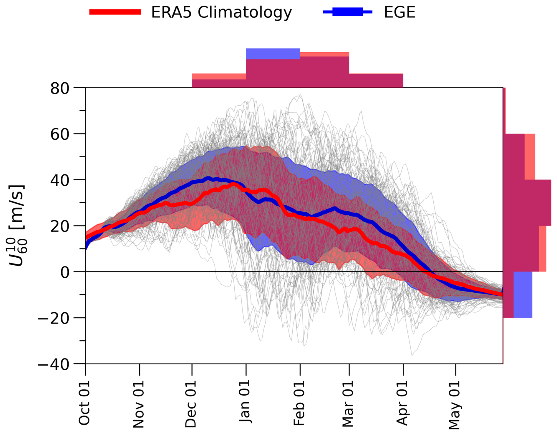
Figure 1 Evolution of the zonal-mean zonal wind at 10 hPa, 60° N in ensemble simulations and reanalysis data. Grey thin lines show the evolution of individual EGE ensemble members, with the EGE ensemble mean shown in blue (thick line). The ERA5 reanalysis climatology for 1980–2019 is shown in red (thick line). Shaded regions indicate climatological variability (±1 standard deviation) for the EGE (blue) and ERA5 (red). Histograms represent winter (December–March) values only, with EGE shown in blue and ERA5 in red. The top panel shows the SSW frequency per month, allocated according to the SSW start date. The right panel shows the distribution of the zonal-mean zonal wind at 10 hPa, 60° N. All histograms are normalized by the respective dataset size (EGE: 120; ERA5: 40).

A set of spin-off ensemble simulations is then performed for 18 selected SSWs identified in the individual members of the EGE. These are initialised with perturbed initial conditions of the corresponding EGE member at the SSW onset or the day before – to minimise resource usage we only store the full atmospheric state every other day – and run for 60 d. Here, d₀ denotes the onset date of the SSW, defined as the first day on which the zonal-mean zonal wind at 10 hPa and 60° N becomes negative (see Sect. 2.2 for details).

Each spin-off ensemble consists of 40 members, with initial ensemble perturbations constructed following the random field perturbation approach described by Magnusson et al. (2009). The random field perturbations use the naturally occurring variability patterns within the climatological dataset of our EGE. To perturb a spin-off ensemble member for a given SSW with onset date d₀, identified in a given EGE member, we compute the difference between the atmospheric states on two randomly drawn days, d₁ and d₂. Here, d₁ and d₂ are drawn from two distinct EGE members other than the member containing the SSW and have to be within a ±15 d window around d₀ to reduce seasonal signals. The difference in atmospheric states at those days is then scaled by a tuning factor adjusted to provide adequate error growth over the first few weeks of the model run. The method for determining this factor is outlined in Magnusson et al. (2009). Each perturbation pattern then creates two members of the spin-off ensemble by adding and subtracting it from the unperturbed initial conditions field, leading to an unchanged ensemble mean. As a result, each spin-off ensemble samples the range of plausible tropospheric evolutions conditional on the same stratospheric event.

This approach of generating spin-off ensembles guarantees that each ensemble member captures the chosen SSW identically, primarily because the ensemble is initialised on the day of the SSW (such that the dynamical event has already occurred), and because the stratosphere exhibits relatively high intrinsic predictability on timescales of up to about two weeks (see e.g., Garny, 2025; Rupp et al., 2023). As a result, the initial (≥ 2 weeks) stratospheric evolution remains very similar across ensemble members. This setup furthermore provides the basis for an improved statistical characterisation of the possible tropospheric evolutions following a stratospheric event, and crucially, enables a direct comparison of conditional tropospheric response distributions across different SSWs. The key advantage of this spin-off ensemble setup can be distilled to the following: While the constructed EGE setup rules out external confounding factors, we cannot deduce from the EGE alone whether the case-to-case variability in the tropospheric evolution following SSWs is driven by the tropospheric variability, or by how strongly an SSW couples downward. This is where the spin-off simulations play a pivotal role, as they allow for the quantification and inter-comparison of event-specific response distributions through the ensemble framework.

We use the ERA5 reanalysis dataset (Hersbach et al., 2020) from the European Centre for Medium range Weather Forecasts (ECMWF) as an observational climatological reference for evaluating our ICON-generated set of possible wintertime evolutions of the coupled troposphere-stratosphere system (i.e., the EGE) in Sect. 3. The climatology is calculated as the average spanning the years 1980–2019. The ERA5 dataset was obtained as output of the reanalysis on a 1° × 1° regular horizontal grid following pressure surfaces and has a 6-hourly temporal resolution.

2.2 Definition of metrics

We identify SSWs as the reversal of the zonal-mean zonal wind at 10 hPa and 60° N ($U_{\mathrm{60}}^{\mathrm{10}}$) and define the SSW onset as the first day the reversal to an easterly wind occurs, following the criteria introduced in Charlton and Polvani (2007). Although all events are conditioned on SSW onset and occur within the winter season, weak residual seasonality in radiative vortex recovery may still modulate post-onset zonal winds. However, SSW identification based on absolute wind reversal ($U_{\mathrm{60}}^{\mathrm{10}}<\mathrm{0}$) constitutes a more stringent criterion earlier in winter. We use the $U_{\mathrm{60}}^{\mathrm{10}}$ index to encapsulate the strength of an SSW and require the zonal-mean zonal wind between two events to recover and remain westerly for 20 consecutive days or more for these to be considered separate SSWs (e.g. Butler et al., 2017). Final warming events (Butler et al., 2015) are excluded from our analyses. We further restrict SSWs to December-February, excluding March events to avoid late-season vortex breakdowns associated with final warmings.

The SSW intensity metric $U_{\mathrm{60}}^{\mathrm{10}}$ is defined as the two-week mean zonal-mean zonal wind at 10 hPa and 60° N following the event onset. As such, it reflects both the magnitude and persistence of the wind reversal rather than an instantaneous amplitude. Absolute values are used, as the zero-wind threshold represents a physically meaningful reference for SSW conditions, largely independent of the timing within the season. Using $U_{\mathrm{60}}^{\mathrm{10}}$ anomalies instead of absolute values yields qualitatively similar results (not shown), indicating that our conclusions are not sensitive to this choice of metric.

We use standardized geopotential height (GPH) anomalies averaged over the polar cap (60–90° N) as a measure of the large-scale zonal circulation in the stratosphere and troposphere when investigating possible stratosphere-troposphere coupling. This metric captures the progression and evolution of downward propagating signals both within the stratosphere and from the stratosphere to the surface. GPH anomalies are standardised with respect to the 120-member EGE, unless stated otherwise. We define the surface response metric as the 1000 hPa GPH anomaly averaged over weeks 3–7 following SSW onset, and the lower stratospheric response metric as the GPH anomaly at 100 hPa. An SSW is classified as exhibiting a lower stratospheric response if the 100 hPa GPH anomaly exceeds 1.5σ for at least 10 consecutive days within the first six weeks after SSW onset. These time ranges are motivated by the timescales typically associated with the downward propagation of stratospheric mean-flow anomalies, spanning days to approximately two months (see e.g., Ding et al., 2023; Scaife et al., 2022; Sigmond et al., 2013), and are further supported by the composite results of this study (e.g., Figs. 3 and 8). We tested the sensitivity to the exact definition of these time ranges, and results are generally robust with respect to variations of a few weeks (not shown). The weeks 3–7 period is therefore chosen to capture the delayed sub-seasonal surface response following SSW onset, while allowing for event-to-event differences in response timing.

To quantify large-scale atmospheric circulation variability we also employ the $\stackrel{\mathrm{̃}}{\mathrm{AO}}$ index, which is calculated as the difference in the zonal-mean GPH at 1000 hPa between the meridional means over 30–50° N and 60–90° N. As detailed in Rupp et al. (2022), this index serves as a proxy for the strength, latitudinal position, and offers the advantage of being computable directly from model output without requiring a long-term climatological baseline for EOF analysis.

To diagnose wave–mean flow interactions in the stratospheric zonal-mean circulation, we employ the Transformed Eulerian Mean (TEM) formulation (Andrews and McIntyre, 1976):

$$\begin{array}{}\text{(1)}& {\displaystyle \frac{\partial \stackrel{\mathrm{‾}}{u}}{\partial t}}=f_{\mathrm{0}}{\stackrel{\mathrm{‾}}{v}}^{\star }+{\displaystyle \frac{\mathrm{1}}{{\mathit{\rho }}_{\mathrm{0}}}}\mathrm{\nabla }\cdot \mathit{F}+\stackrel{\mathrm{‾}}{\mathit{X}}\end{array}$$

The Eliassen-Palm (EP) flux F is defined in terms of eddy momentum and heat fluxes, and provides a way to portray the origin and impact of waves on the zonal mean flow. In Eq. (1), the EP-flux divergence appears as an explicit wave-induced forcing term, quantifying the net momentum transfer from propagating waves to the mean flow. Physically, EP-flux convergence corresponds to a westward (decelerating) force on the mean zonal wind due to breaking and dissipation of planetary waves. In Eq. (1), this corresponds to negative ∇⋅F, which contributes to decelerating the stratospheric westerly jet. This formalism elucidates the fact that the stratospheric momentum balance is fundamentally controlled by wave drag: stratospheric conditions, such as the strength of the polar vortex, are strongly coupled to planetary wave activity in the lower stratosphere, consistent with previous findings (see also, e.g. Birner and Albers, 2017; Dunn-Sigouin and Shaw, 2015).

Blocking detection is done for a latitude band of 60 to 75° N around the Northern Hemisphere using the two dimensional blocking index by Scherrer et al. (2006), resulting in a binary gridpoint-wise blocking occurrence. The index is calculated for every central latitude (Φ₀) between 45 and 75° N using the southern and northern GPH gradient at 500 hPa:

$$\begin{array}{}\text{(2)}& {\displaystyle }\mathrm{GHGS}={\displaystyle \frac{Z\left({\mathrm{\Phi }}_{\mathrm{0}}\right)-Z\left({\mathrm{\Phi }}_{\mathrm{s}}\right)}{{\mathrm{\Phi }}_{\mathrm{0}}-{\mathrm{\Phi }}_{\mathrm{s}}}}\text{(3)}& {\displaystyle }\mathrm{GHGN}={\displaystyle \frac{Z\left({\mathrm{\Phi }}_{\mathrm{n}}\right)-Z\left({\mathrm{\Phi }}_{\mathrm{0}}\right)}{{\mathrm{\Phi }}_{\mathrm{n}}-{\mathrm{\Phi }}_{\mathrm{0}}}}\end{array}$$

with ${\mathrm{\Phi }}_{\mathrm{n}}={\mathrm{\Phi }}_{\mathrm{0}}+\mathrm{15}$° N and ${\mathrm{\Phi }}_{\mathrm{s}}={\mathrm{\Phi }}_{\mathrm{0}}-\mathrm{15}$° N. A given latitude-longitude grid-point is defined as blocked when the following conditions are satisfied: GHGS>0 and $\mathrm{GHGN}<-\mathrm{10}$ m per degree lat. In this paper we show the blocking frequency anomalies (with respect to climatology) averaged over weeks 3–7 after the onset of the SSW.

The statistical significance of the difference in means is determined using the one-sided two-sample Student's t-test on a 95 % confidence level. We compare the variances of ERA5 and the EGE using a sample-size adjusted Fisher's F-test. To measure the strength of the linear association between metrics presented in this paper we use the standard Pearson correlation coefficient, denoted by r.

3 Composite mean downward impact of SSWs in the Event-Generating Ensemble

As detailed in Sect. 2, the 120-member ensemble simulation provides a large set of possible evolutions of the coupled troposphere-stratosphere system during winter months (see Fig. 1). The ICON climatology of stratospheric polar vortices follows that of ERA5 well (Fig. 1), and the number of SSWs produced by the EGE is similar to that of the ERA5 climatology (Butler et al., 2017): Out of the 120 members, 57 developed SSWs in December-February; the majority of which occur in January and February (Fig. 1). The EGE controlled conditions suppress differences between ensemble members in terms of interannual variability (e.g. QBO, MJO, ENSO) despite the independent stratosphere-troposphere evolution. We expect a smaller variability in the EGE dataset. However, the interannual variability becomes indistinguishable from that of ERA5 after the first month, suggesting an important role of internal variability for the polar vortex. This also indicates that initial condition memory has subsided from November onwards, such that individual ICON ensemble members can be treated as independent winter evolutions.

The distinct evolution of the stratospheric warming events compared to the modelled climatological progression (Fig. 2a) allows the potential downward influence of SSWs to be examined: Fig. 2b highlights the significant anomaly in the composite mean tropospheric zonal-mean circulation beginning two weeks after SSW onset, consistent with observations and previous work (see e.g., Baldwin and Dunkerton, 2001; Lee et al., 2019; Spaeth and Birner, 2022). This tropospheric signal of negative $\stackrel{\mathrm{̃}}{\mathrm{AO}}$ index anomalies remains statistically significant for up to five to six weeks following the SSW onset. For the climatological reference shown in Fig. 2a, day 0 corresponds to randomly selected winter dates (January–February) within each EGE member, such that the time axis represents lag days relative to a random reference date. Figure 3 shows the downward progression of the anomalies after SSWs in terms of average polar cap GPH. Selecting only events with a lower stratospheric anomaly highlights that the state of an anomalous lower stratosphere influences the strength of the surface response following an SSW event, consistent with previous work (see e.g. Hitchcock et al., 2013 and others in Sect. 1). The lower stratospheric anomalies were classified as anomalously strong if the GPH anomalies at 100 hPa exceeded values of 1.5σ for at least 10 d within the 6-week period after SSW onset (see Sect. 2.2). As shown in Fig. 3b, the SSWs displaying this lower stratospheric signal show a clear increase in the large-scale tropospheric surface anomaly in the weeks following the SSW. Furthermore, the increased surface anomalies differ significantly from the remaining SSW members not satisfying the lower stratospheric threshold (see Fig. S2 in the Supplement).

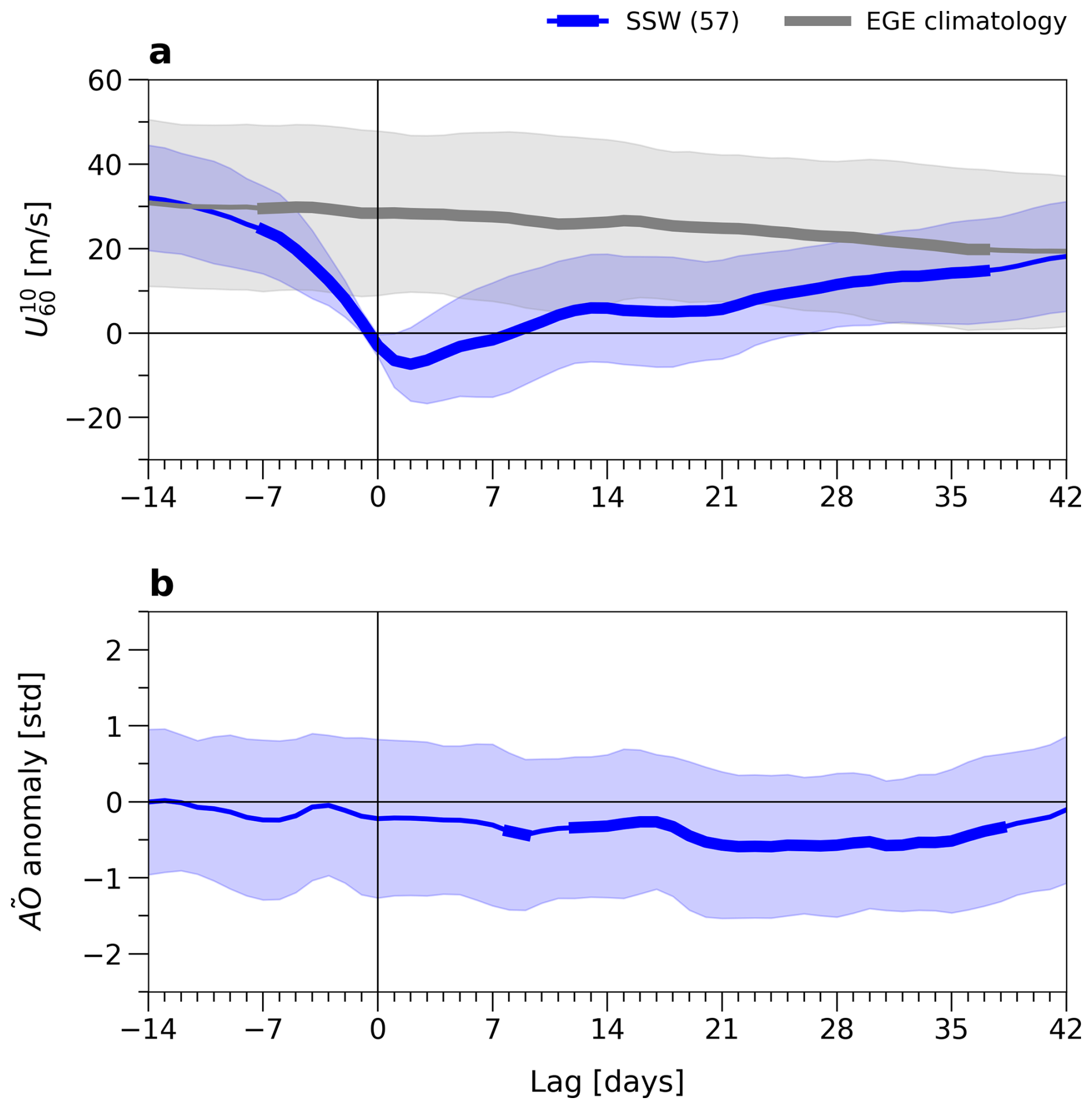
Figure 2 Lagged time series of (a) the zonal-mean zonal wind at 10 hPa, 60° N for the EGE climatology (grey) and SSW composite (blue), and (b) $\stackrel{\mathrm{̃}}{\mathrm{AO}}$ anomalies for the SSW composite (blue). The climatology is calculated as the EGE ensemble mean. For the climatological reference, day 0 corresponds to randomly selected winter dates (January–February) within each EGE member, such that the time axis represents lag days relative to a random reference date. For the SSW composite, day 0 corresponds to the SSW onset and is marked by the thin black vertical line. Thickened line segments indicate periods during which the difference in means between the SSW composite and climatology is statistically significant at the 95 % confidence level, with shaded envelopes indicating the ensemble spread (±1 standard deviation). $\stackrel{\mathrm{̃}}{\mathrm{AO}}$ anomalies for the climatology are not shown, as their climatological mean is zero. The number of EGE members included in the SSW composite is indicated in brackets.

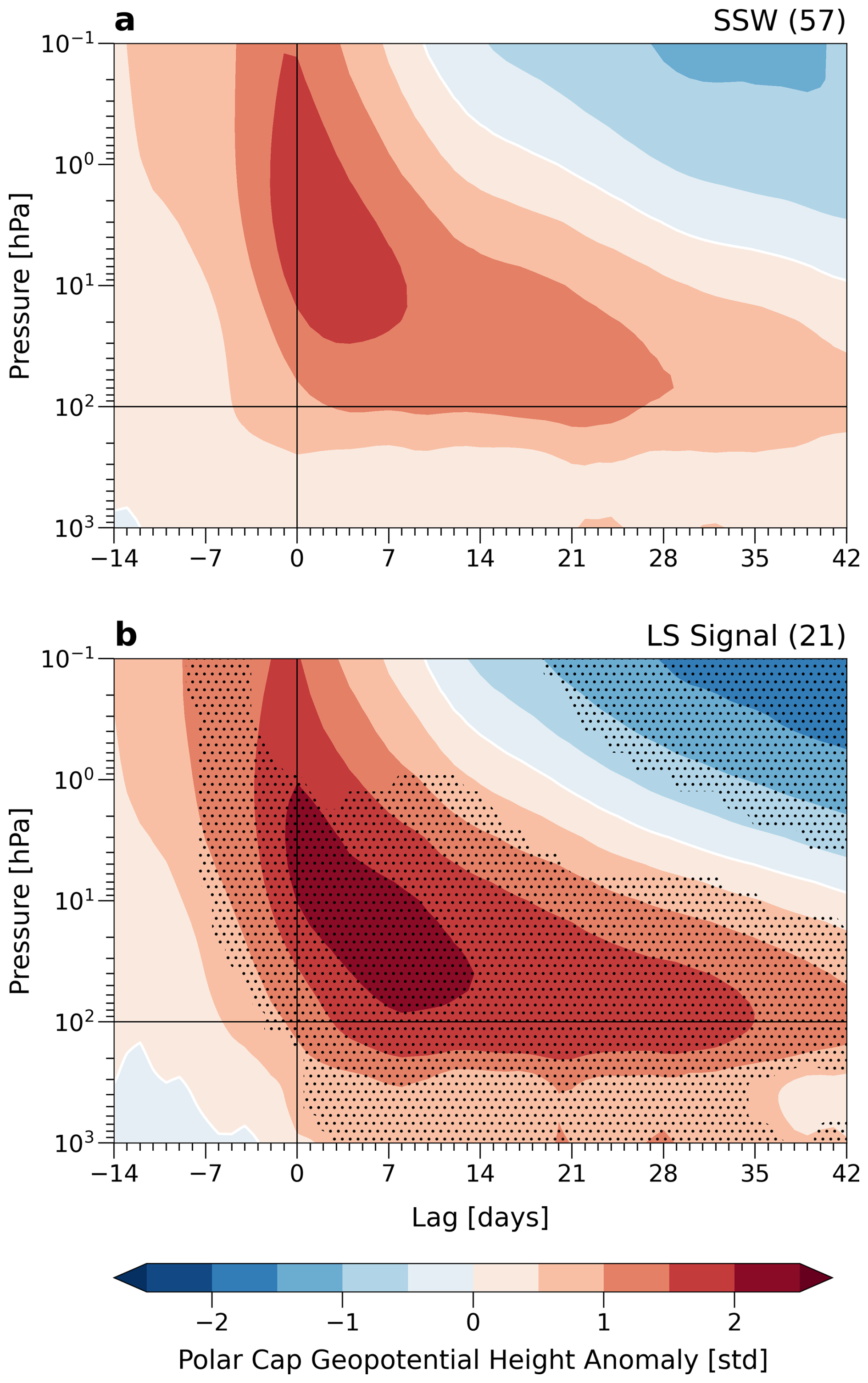
Figure 3 Event-based composite of GPH anomalies of (a) all SSWs identified in the EGE and (b) events with a strong LS signal following the SSW. Numbers in the panel headings represent group sizes. Stippling indicates significant differences at the 95 % confidence level in cluster means between events with an LS signal and those without (not shown, see Fig. S1). Thin black lines in the vertical and horizontal directions mark the start of the SSW and the 100 hPa pressure level, respectively.

With the aim of quantifying shifts in the probability of anomalous tropospheric zonal-mean circulation patterns, probability density functions (PDFs) and distributions of daily GPH anomalies are compared in Fig. 4 for weeks 3–7 following the stratospheric event. Consistent with the findings of Baldwin and Dunkerton (2001), pronounced differences in tropospheric anomalies are evident between the composite means of the SSW group (“SSW”) and EGE members without SSWs (“No SSW”). The mean tropospheric GPH anomaly for the SSW group is 0.36±0.97 [standardised], compared to $-\mathrm{0.2}\pm \mathrm{0.97}$ for the No-SSW group. Differences in the shapes of the PDFs further highlight changes in the likelihood of anomalous tropospheric circulation regimes. Values exceeding +2 standard deviations at 1000 hPa are at least twice as likely for the “SSW”-group, consistent with estimates of attributable risk reported by Spaeth and Birner (2022). Conversely, values below −2 standard deviations at 1000 hPa are more than twice as likely to occur for the “No-SSW”-group. The enhanced tropospheric anomalies associated with the LS-signal cluster, previously shown in Fig. 3b, are also clearly visible in Fig. 4a, both as a rightward shift of the PDF (upper panel) and in the box-and-whisker plots (lower panel). This shift peaks approximately four weeks after SSW onset (not shown). Surface anomalies exceeding +2 standard deviations are more than four times as likely in the LS-signal group than in the “No SSW”-regime, while SSWs without a lower stratospheric signal are at least twice as likely (green). The latter group behaves similarly to the modelled climatology in terms of both composite means and the tails of the PDFs. In the lower stratosphere, positive anomalies are likewise more likely following SSWs, as indicated by the distributional shift shown in Fig. 4b.

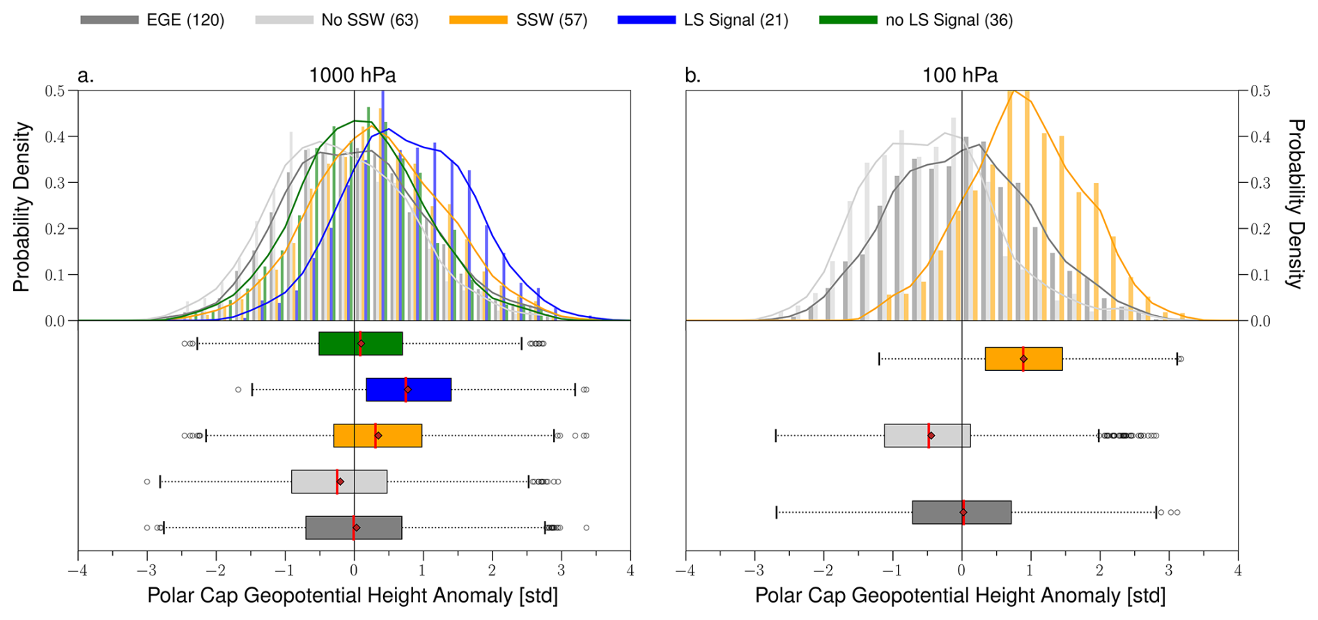
Figure 4 Probability density functions (top panels) and distributions (bottom panels) of standardised GPH anomalies for weeks 3–7 following the event date at (a) 1000 hPa and (b) 100 hPa from the EGE simulation. Dark grey shows the climatology, light grey members without SSWs, and yellow members with SSWs. Among SSWs, events with and without a lower-stratospheric signal are shown in blue (LS) and green (noLS), respectively. Red diamonds and vertical lines indicate the mean and median, respectively, with sample sizes given in brackets. Anomalies are defined relative to the EGE climatology (120-member ensemble mean). For the climatology and No-SSW groups, the event date corresponds to a randomly selected January–February day. Boxplots show the interquartile range (25th–75th percentiles), with whiskers extending to 1.5 times the interquartile range; values beyond this range are shown as outliers.

Overall, our analyses of the EGE show a downward influence of SSWs on the tropospheric flow in the composite mean, in agreement with the well-known signal first described in Baldwin and Dunkerton (2001). Our analyses further confirm that the EGE ensemble successfully captures the important role of the lower stratosphere for downward coupling, in agreement with previous studies (see Sect. 1), pointing towards the lower stratosphere acting as a mediator between the upper/mid-stratosphere (SSW) and the troposphere. Based on our findings from the composites of SSWs, we utilize the spin-off ensembles in the next Section to examine whether the development of a lower stratospheric anomaly is more or less likely to develop for individual SSWs, and whether this determines the likelihood for a tropospheric response to develop.

4 Selecting SSW events for Spin-off Ensembles

The selected SSWs for which we conducted spin-off ensemble simulations, cover the range of possible stratospheric SSW evolutions in terms of extremity and timing throughout the winter months from December to February. For each spin-off, Fig. 5 shows the stratospheric conditions post-SSW in terms of the $U_{\mathrm{60}}^{\mathrm{10}}$ index averaged over the first two weeks of the selected event.

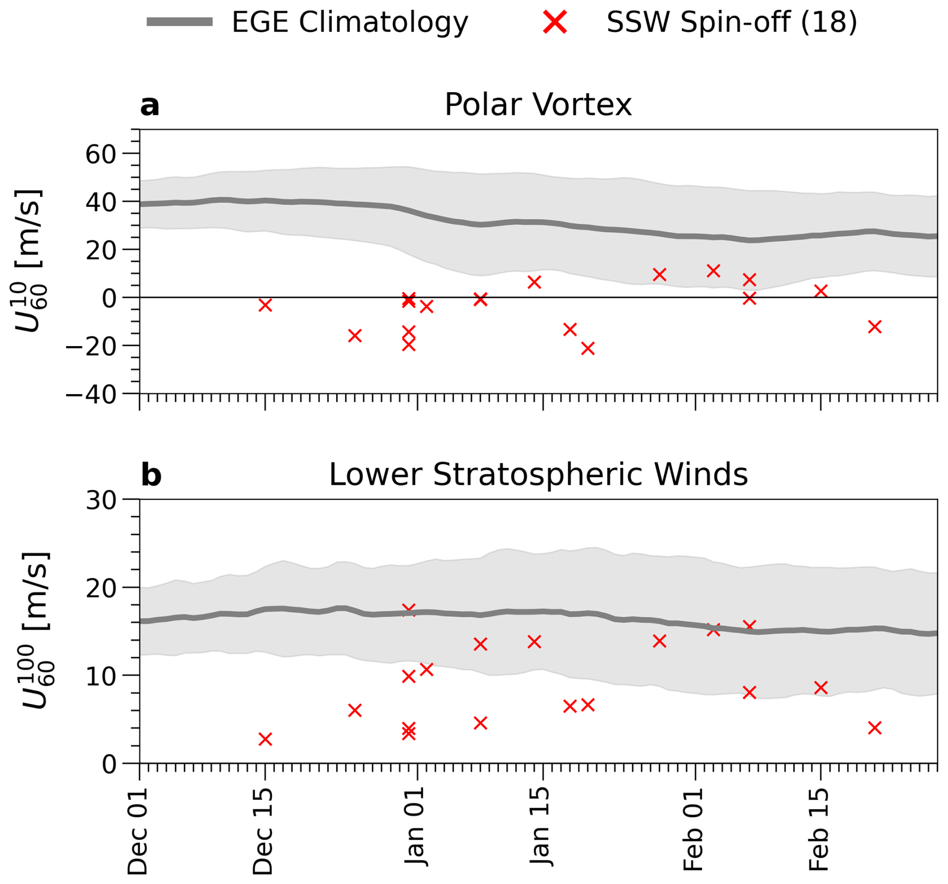
Figure 5 Overview of post-SSW stratospheric conditions in terms of (a) polar vortex strength, defined as the zonal-mean zonal wind at 10 hPa and 60° N, and (b) lower stratospheric winds, defined as the zonal-mean zonal wind at 100 hPa and 60° N, both averaged over the first two weeks after SSW onset, for the spin-off ensemble simulations based on SSWs (red crosses) during the winter months from December to the end of February. The thick line represents the EGE ensemble mean, with ±1 standard deviation shown as shading.

In addition to covering a broad range of post-SSW states in the stratosphere, the SSW spin-off simulations also capture the range of possible coupled stratosphere-troposphere evolutions (Fig. 6). As expected, the majority lie in the lower right quadrant, as observational data has shown that SSWs are linked to increased surface GPH anomalies (i.e. negative anomalies on the y-axis and positive anomalies on the x-axis in Fig. 6; see e.g. Kautz et al., 2020). The upper left and right quadrants capture brief or weak warming events that are followed by negative or positive (i.e. weak to strong) tropospheric signals, respectively. Figure 6 further contrasts the selected EGE members with the ensemble mean over the 40 spin-off ensemble members (coloured crosses and dots). Note that for each selected event, the selected EGE member represents one of the 40 members of the spin-off and the stratospheric state is very similar: The deterministic state lasts up to 10 d and the state is shown here averaged over the first 14 d. We see a greater difference in the values from the selected SSW of the EGE and the spin-off ensemble mean in terms of the tropospheric surface response index, as this index captures the surface state several weeks after initialisation once all members have evolved separately, which again emphasises the key advantage of the spin-off ensemble simulation setup.

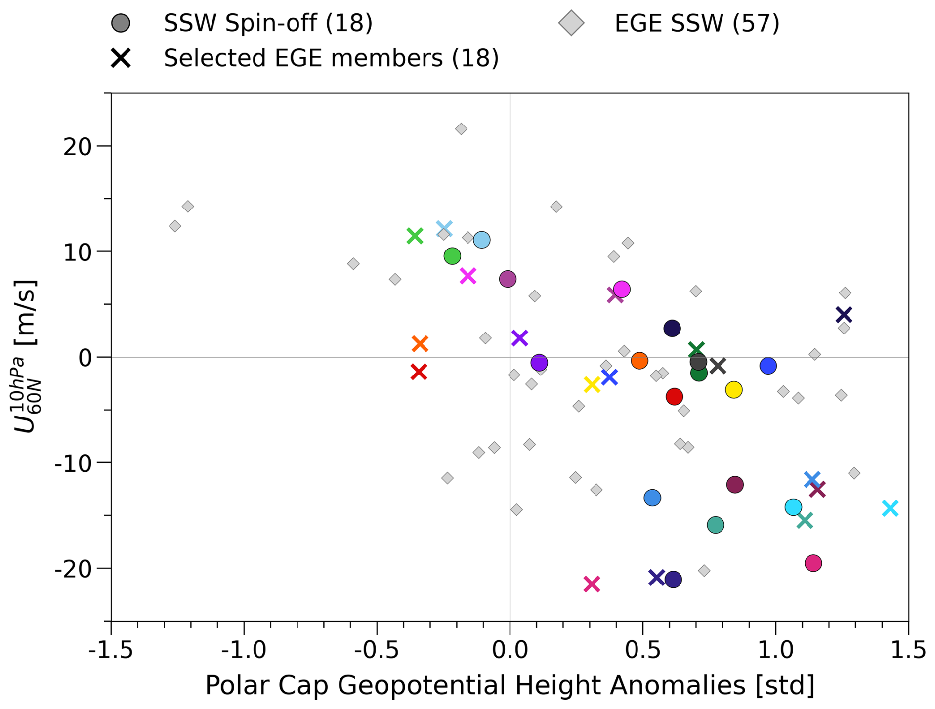
Figure 6 Overview of selection of SSW spin-offs (circles, different colours) in terms of the zonal-mean zonal wind at 10 hPa, 60° N averaged over the first two weeks and the tropospheric surface response index in the weeks after SSW onset. The 57 SSWs from the event-generating EGE are shown as diamonds. Of these, the EGE members selected for the initialisations of the spin-offs are marked separately with crosses and are shown in the corresponding spin-off colour. The number of members per group is shown in the brackets. Note that zonal-mean zonal winds are shown as two-week averages following SSW onset; positive values reflect the beginning of post-SSW recovery in some events.

5 Differences in downward coupling in selected SSW events

In Sect. 3 we showed that our ICON EGE simulations reproduce the known downward influence of SSWs on the tropospheric flow and established that on average across events, a persistent weakening of the zonal circulation in the lowermost stratosphere following the SSWs increases the likelihood for tropospheric flow anomalies to occur. In this section we analyse if the forced SSW impact onto the troposphere is strongly related with the 100 hPa stratospheric anomaly, and whether it is case dependent.

Figure 7 presents the ensemble distribution of standardised GPH anomalies averaged over 3 to 7 weeks after SSW onset at the surface (Fig. 7a.) and lower stratosphere (Fig. 7b.) for all SSW spin-offs. The results at 1000 hPa illustrate the varyingly positive surface responses in the ensemble mean for the SSWs, in line with Fig. 6. For this reason, we can conclude that across individual SSWs, some are more likely than others to develop a tropospheric response in the aftermath of the stratospheric event. This is an important result because it suggests that the differing tropospheric evolutions observed following SSWs – where some events exhibit the canonical response while others do not – may not be attributable solely to internal tropospheric variability (i.e. chance). Instead, there is predictive information available at the time of SSW onset regarding the likelihood of a given SSW developing a tropospheric response. At the same time, the broad distributions of the ensemble response confirm that the tropospheric response to an individual SSW cannot be inferred from a single observed realisation: even for SSWs with a strong ensemble-mean response, some individual members exhibit negative time-averaged tropospheric anomalies.

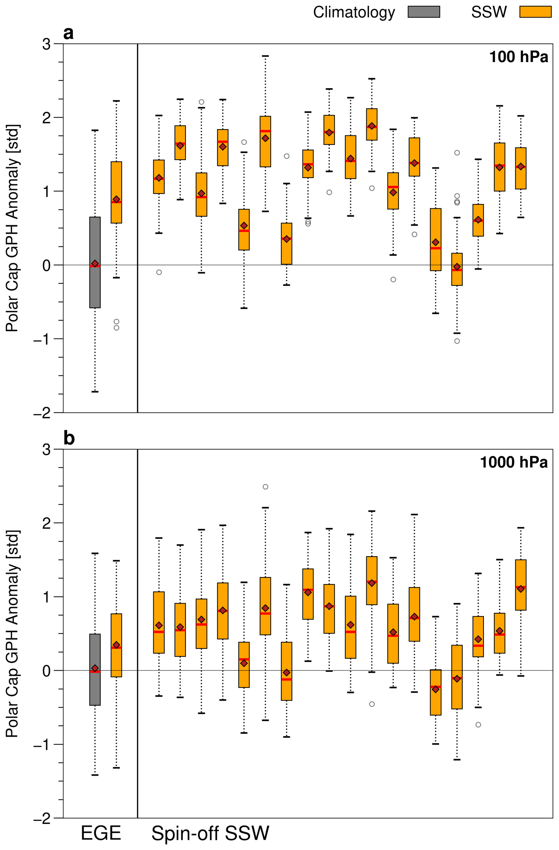
Figure 7 Distribution of standardised GPH anomalies at (a) 100 hPa and (b) 1000 hPa, averaged over weeks 3–7 post-event. In each panel, the left side shows values for the EGE (as in Fig. 4), while the right side shows all spin-off simulations. Colours follow Fig. 4: the EGE ensemble mean is shown in dark grey, and yellow denotes the composite mean of the EGE SSWs (left) and the spin-off ensemble mean (right). Red diamonds indicate the mean and vertical lines the median. Boxplots show the interquartile range (25th–75th percentiles); whiskers extend to 1.5 times the interquartile range, with points beyond classified as outliers.

One might suspect that stronger wind reversal events in the stratosphere have stronger surface impacts, and vice versa, but this is not generally the case as illustrated in Fig. 8 for three example events. While the spin-off ensemble simulation “SSW 1” captured both a strong warming event as well as a strong surface response in the ensemble mean (Fig. 8a and d, respectively), the correspondingly weak event in spin-off “SSW 3” (Fig. 8, third column) shows no evidence of downward coupling in the ensemble mean. Another equally weak SSW in terms of a stratospheric reversal of winds (“SSW 2”, middle column) develops positive surface anomalies of comparable magnitude with those of the strong event “SSW 1”. While one could first assume this difference relates to the strength of the SSW, a clear link between the event strength and surface response is visible only to a limited extent (see also e.g. Fig. 10b). However, the evolution of the lower stratosphere points towards the importance of an anomalous state at 100 hPa for a surface signal to develop (compare “SSW2” to “SSW3”). Moving beyond these three examples in Fig. 8 and considering the full set of spin-off ensemble simulations, we indeed observe that the ensemble mean response in the lower stratosphere does differ substantially between the SSWs, cf. Fig. 7b. We corroborate this with Fig. 9, in which the ensemble mean GPH anomaly at different times and heights is correlated against the ensemble mean surface response (averaged over week 3–7) across the 18 spin-offs. Here, a weaker correlation of the surface response with GPH anomalies at 10 hPa than with those at 100 hPa is found. Most notably, the surface response can be considered highly correlated with the GPH anomaly at 100 hPa from week 2 onwards, as the composite correlation coefficient exceeds 0.8 and approaches maximum values. This correlation peak in the lower stratosphere appears before the surface signal develops, and notably is stronger compared to the correlation of the surface signal with anomalies in the upper troposphere (around 400 hPa).

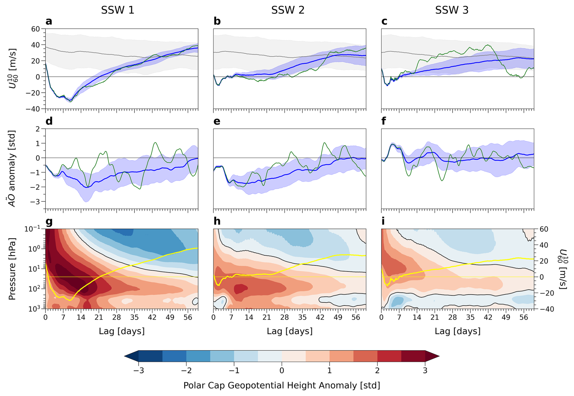
Figure 8 Time series of the zonal-mean zonal wind at 60° N and 10 hPa (a–c), AO anomalies (d–f), and standardised GPH anomalies (g–i) for selected spin-off simulations. Each column corresponds to a distinct SSW. In panels (a)–(f), spin-off simulations (blue) are based on selected SSWs from the EGE (green). The EGE climatology (120-ensemble mean) and standard deviation are shown by the grey line and shading, respectively. In panels (g)–(i), the ensemble mean zonal-mean zonal-wind at 60° N and 10 hPa is overlaid as a yellow line. Day 0 denotes the onset of the SSW.

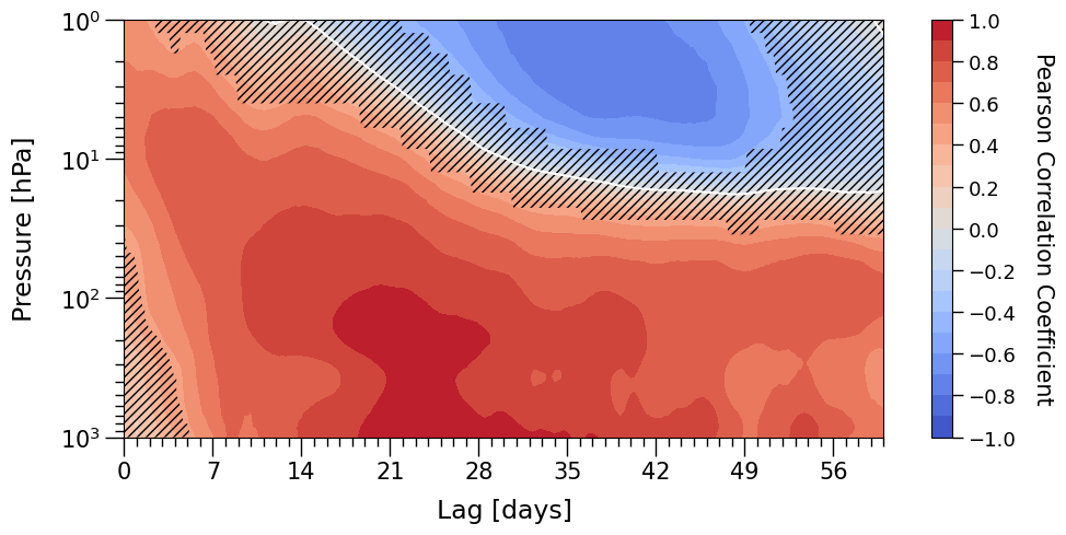
Figure 9 “Dripping paint” plot of the spin-off ensemble composite Pearson correlation between GPH anomalies and the week-3–7 averaged 1000 hPa GPH anomalies. Stippling denotes non-significant correlations (p>0.05).

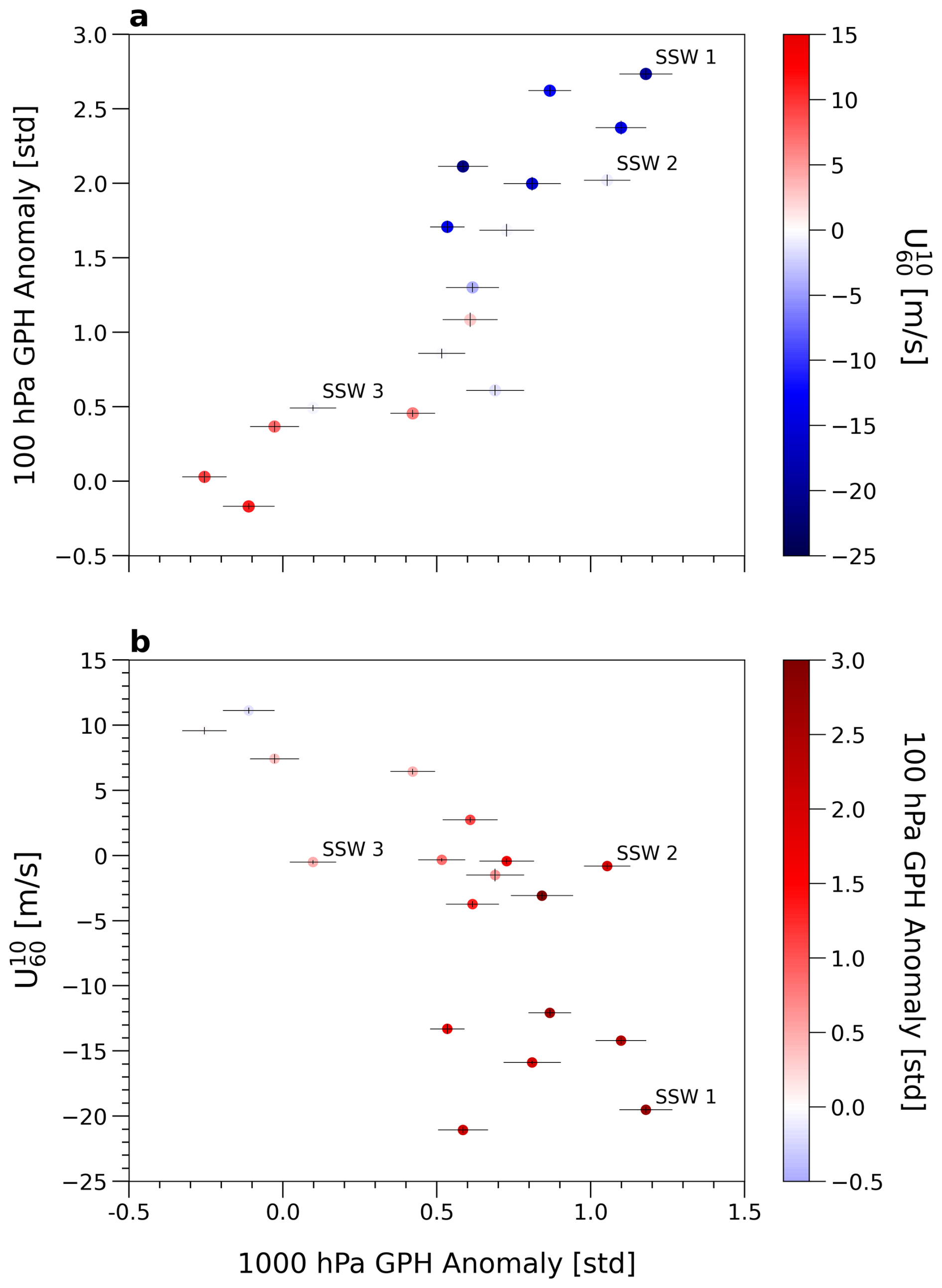
Figure 10 Scatter plot showing the relationship between 1000 hPa GPH anomalies and (a) week-2 mean 100 hPa GPH anomalies and (b) the post-SSW vortex strength, quantified by the two-week mean $U_{\mathrm{60}}^{\mathrm{10}}$, across the ensemble means of all 18 spin-off ensembles. Each ensemble mean point is coloured according to (a) the two-week mean $U_{\mathrm{60}}^{\mathrm{10}}$ or (b) the 100 hPa GPH anomaly, as indicated by the colour bars. Error bars depict the standard error of the ensemble mean. The corresponding correlation coefficients are: (a) r=0.85 (p<0.001) and (b) $r=-\mathrm{0.71}$ (p<0.01).

Previously we established that the occurrence of a 100 hPa anomaly plays a key role in whether we see downward coupling across the SSW-composite mean (see Fig. 4). Figure 10 now summarizes and underlines the relationship between the state of the lower stratosphere and the strength of the tropospheric surface signal across events. The lower stratospheric GPH anomalies in the second week after SSW onset display a particularly strong relationship with the surface anomalies averaged over weeks 3 to 7, with a Pearson correlation coefficient of 0.85 (Fig. 10a), which is statistically significant (p<0.01). In comparison, the relationship between the surface anomalies and post-SSW vortex strength, quantified by the two-week mean zonal-mean zonal wind at 10 hPa and 60° N, is also substantial, with a negative correlation coefficient of −0.71 (Fig. 10b) and statistically significant (p<0.01). This metric reflects the magnitude and persistence of the post-SSW vortex rather than an instantaneous amplitude. While both metrics are clearly related to the surface response, the lower-stratospheric state exhibits a stronger relationship across events. This correlation with lower stratospheric anomalies is strong for an extended period post-SSW (see Fig. 9), but becomes strong already in week two after the event (Fig. 10). The anomaly in the lower stratosphere in week two is distinct between individual events, and can be predicted quasi-deterministically at the SSW onset (small spread across ensembles, see Figs. 10 and 7a). Thus, overall we can conclude that individual SSWs are distinct and predictable in their development of a lower stratosphere anomaly, and that this anomaly is closely correlated with the likelihood to develop a zonal-mean tropospheric response thereafter.

Given that the strength of the lower stratospheric anomaly is of critical importance, but not uniquely linked to the SSW strength itself, the question arises which dynamical mechanisms lead to (or prevent) the development of the lower stratospheric anomaly. While we do not intend to fully answer this question, we explore possible mechanisms in Sect. 7. Before, we turn to the question whether the distinct zonal-mean tropospheric response also transfers to distinct regional impacts.

6 Differences in the regional tropospheric impact in selected SSW events

Subsequent to the analysis of the zonal-mean, regional effects are examined to assess whether the differences in zonal-mean downward coupling between events are reflected in variations in regional impact. Both the EGE and spin-off ensemble simulations produce a surface response pattern consistent with the well-documented general surface response to SSWs (Baldwin et al., 2021). This is evident in Fig. 11b–e, showing close to zonally symmetric, positive mean sea level pressure anomalies (MSLP) over the polar cap in weeks 3–7 after SSW onset. The EGE composite signal (Fig. 11b) compares generally well with the composite constructed based on ERA5 (Fig. 11a, see also Fig. S3 in the Supplement). Notably, the composite of SSWs from the spin-off ensemble simulations (Fig. 11c) not only exhibits slightly stronger anomalies over the polar cap but also shows enhanced statistical significance compared to the EGE composite. This key advantage of the spin-off ensemble approach presented in this study becomes evident when comparing overall statistically significant regions: the spin-off composite (18 events) covers a broader area and exhibits stronger signals than the composite derived from an equal number of selected EGE events. The 18 spin-off SSWs are further classified based on the anomalous state of the lower stratosphere two weeks after SSW onset, using the 100 hPa GPH anomaly threshold of 1.5σ (cf. Fig. 9 and Sect. 2). The surface signal intensifies for events associated with a stronger lower stratospheric state (Fig. 11d), both in terms of signal strength as well as the size of the region covered.

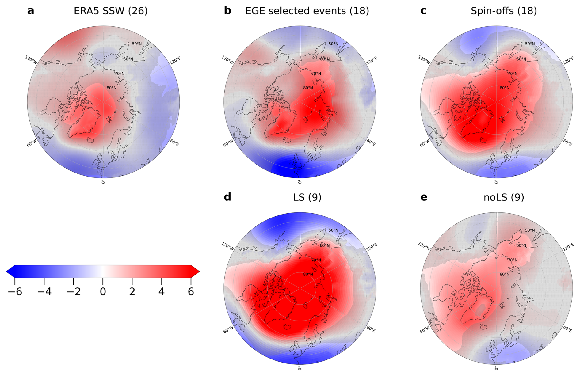
Figure 11 Mean sea level pressure anomalies averaged over weeks 3–7 after SSW onset for composites of: (a) ERA5 SSWs; (b) selected EGE SSWs (18); (c) spin-off SSWs (18), (d) spin-off SSWs with a lower-stratospheric anomaly (LS); and (e) spin-off SSWs without lower-stratospheric anomaly development (noLS) in week 2 after onset. Stippling indicates regions not statistically significant at the 95 % confidence level. Maps are shown in a North Polar Stereographic projection north of 45° N, centred at 90° N, with 10° graticule spacing.

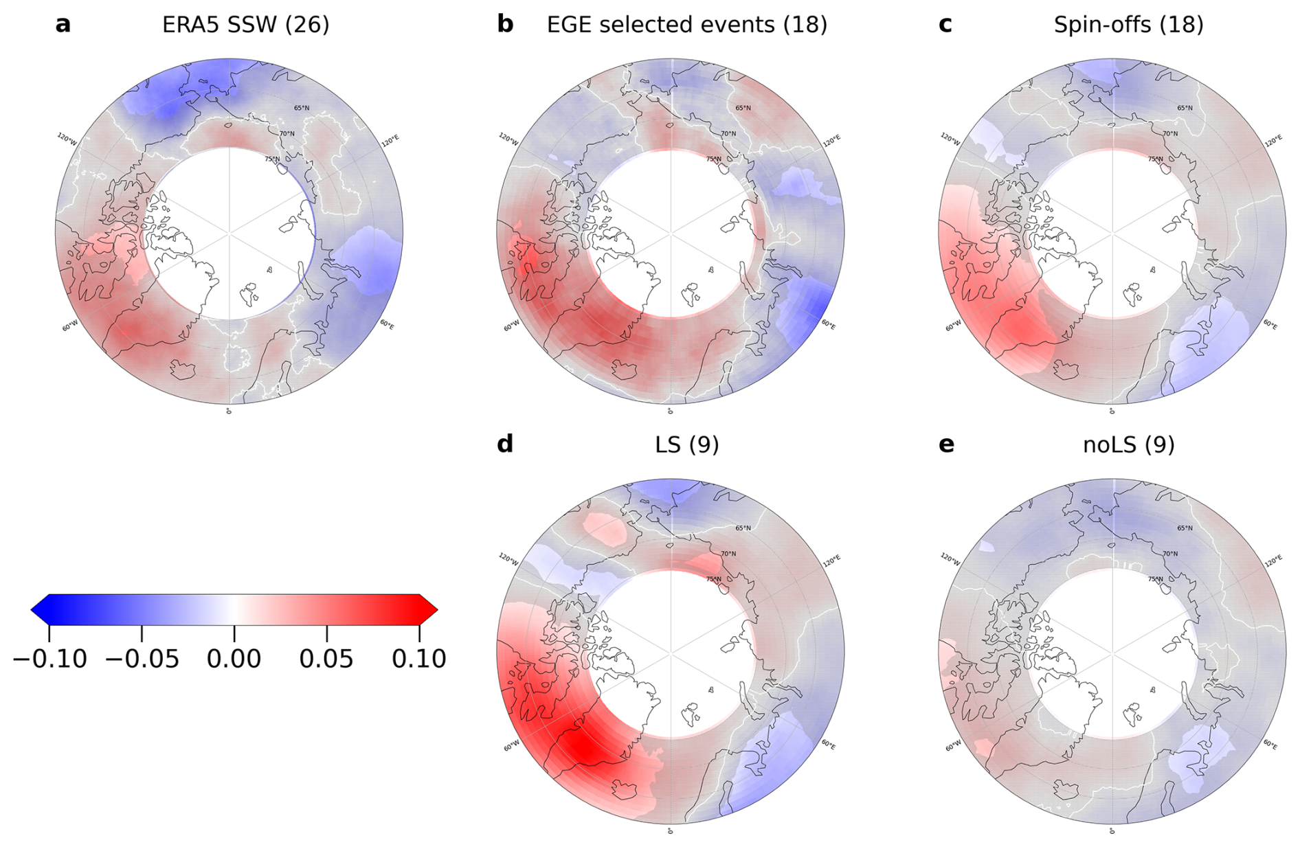
Figure 12 Blocking Frequency Anomalies, defined as the mean number of blocking days averaged over weeks 3–7 after SSW onset. Shown are composite anomalies for (a) ERA5 SSWs, (b) selected EGE events, (c) spin-off ensemble simulations, and spin-off members with (d; LS) and without (e; noLS) strong lower-stratospheric anomalies following the event. Numbers in parentheses indicate the number of members in each composite. Anomalies are calculated relative to the corresponding climatology for each group (e.g. ERA5 SSW composites relative to the ERA5 climatology). Stippling indicates regions not statistically significant at the 95 % confidence level.

In both ERA5 (Fig. 12a) and ICON (Fig. 12b–e), atmospheric blocking frequency in weeks 3–7 following SSW onset shows positive anomalies over Greenland and surrounding regions, consistent with previous work (Lu et al., 2021; Lee et al., 2019; Beerli and Grams, 2019). The spin-off simulations capture statistically significant increases in Greenland blocking, particularly around the Davis Strait, Greenland, and Baffin Island, with frequency values reaching 0.05 (approximately 4 d per season). The enhanced statistical significance in the spin-off SSW composite (Fig. 12c) further underscores the benefits of this simulation approach. Analogous to Fig. 11d, the blocking signal strengthens when selecting SSWs by lower stratospheric anomalies: cases with strong anomalies show a more than twofold increase in blocking frequency over Greenland compared to the spin-off composite, exceeding 0.1 (about 9 d per season) in Fig. 12d.

Given the statistically significant Greenland blocking signal, we compute the correlation between large-scale zonal-mean surface anomalies and regional Greenland blocking frequency, finding a strong correlation of 0.84 (Fig. 13). The correlation between lower stratospheric (100 hPa) anomalies and blocking frequency is slightly lower but remains distinct (0.71). Notably, spin-off events with weak lower stratospheric anomalies (<1.5σ, blue shading) and strong anomalies (>1.5σ, red shading) show an almost full separation (see Sect. 8 for more details). These results highlight the near-linear and strong connection between large-scale zonal mean flow anomalies and regional blocking occurrence, though causality remains uncertain. Individual realisations of post-SSW evolutions from the EGE do not produce any correlation across the SSWs (see Fig. S4 in the Supplement), which again emphasizes that an ensemble is needed to robustly quantify the response.

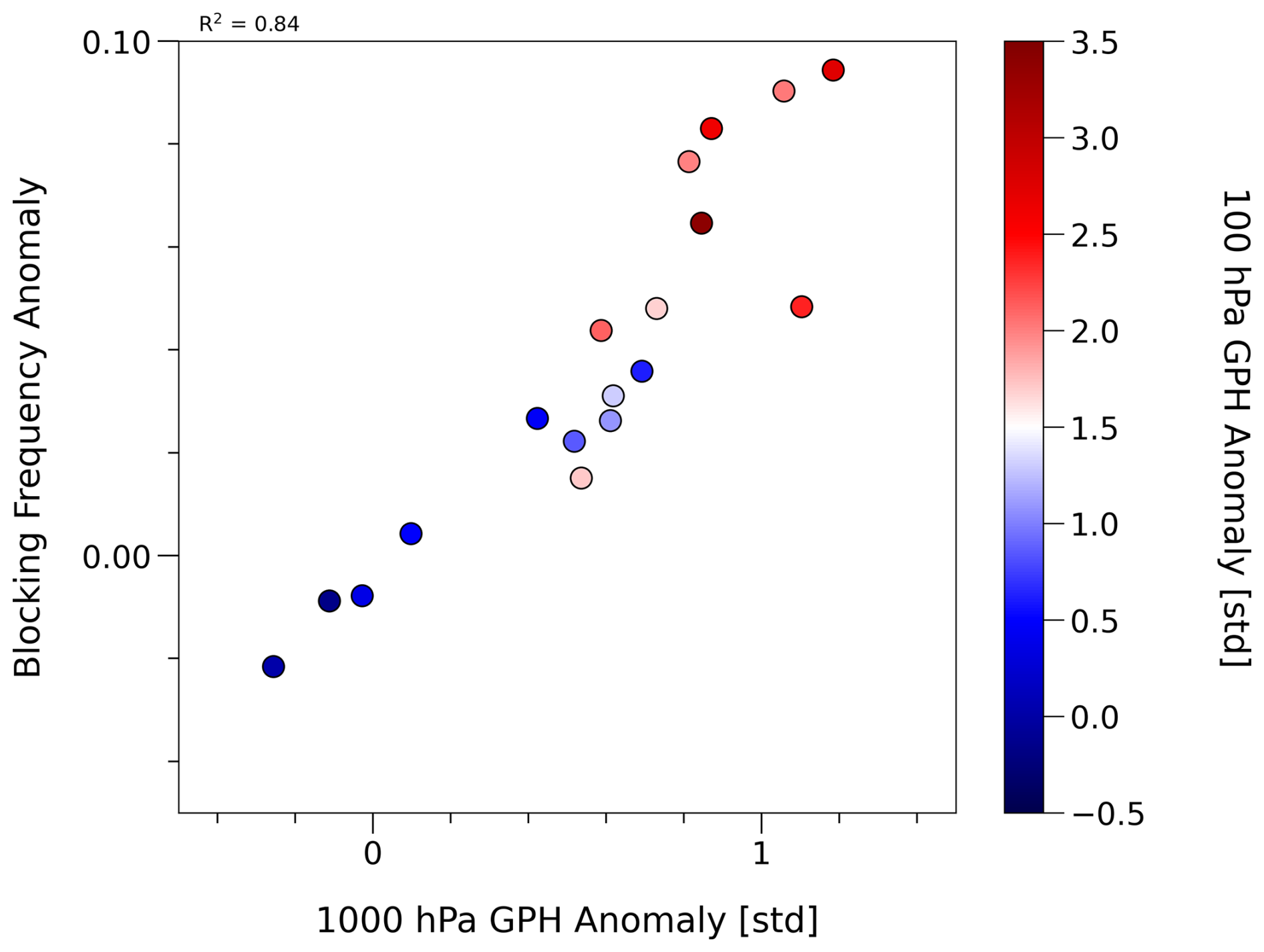
Figure 13 Scatter plot showing the correlation between ensemble-mean 1000 hPa GPH anomalies and the total number of blocking days for the 18 spin-offs over 60–75° N and −90–30° E. Points are coloured by the 100 hPa GPH anomaly in week 2 after SSW onset.

7 Toward a mechanistic understanding of why not all SSWs lead to lower stratospheric anomalies

As presented in Sect. 5, the evolution of an anomalous state in the lower stratosphere is instrumental in whether a surface signal develops, but the strength of the lower stratospheric anomaly is not necessarily linearly linked to the strength of the wind reversal at 10 hPa. In the following, we discuss possible mechanisms that might prevent the development of lower stratospheric anomalies on the example of three SSWs. While we have examined diagnostics related to wave reflection across a broader set of events, substantial case-to-case variability and strong temporal dependence make it difficult to define a single objective metric for a systematic classification; we therefore focus here on three representative cases to illustrate possible mechanisms.

Since the post-SSW stratospheric evolution is governed by interactions between planetary waves and the zonal mean flow, we use the transformed Eulerian mean (TEM) framework to interpret the evolution of lower stratospheric wind anomalies and to diagnose processes that may favour – or inhibit – the development of lower stratospheric flow anomalies. Consistent with the established understanding of polar vortex dynamics, we find that the lower stratospheric zonal-mean zonal wind is strongly correlated (r=−0.91) with GPH anomalies at the same level (not shown), indicating that both diagnostics provide a coherent measure of the evolving vortex state in our framework.

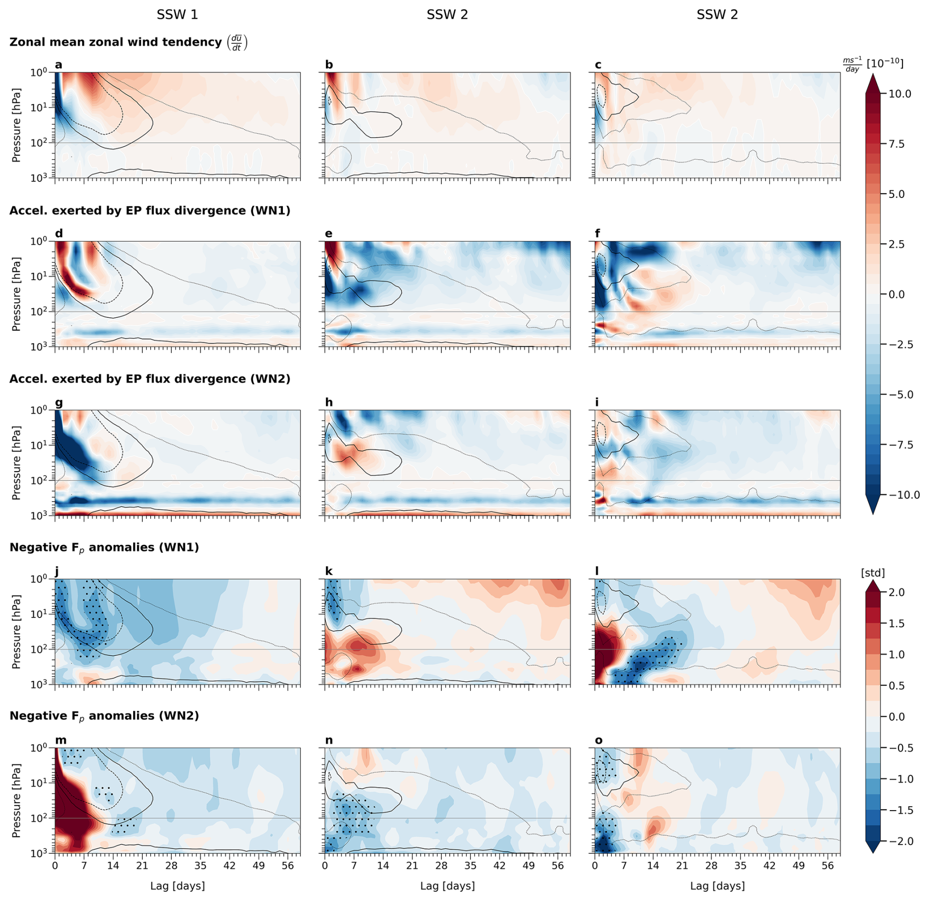
Figure 14 Major terms from the TEM momentum budget and EP-flux diagnostics for the three SSWs shown in Fig. 8. Zonal-mean zonal wind tendency is shown in panels (a)–(c), acceleration exerted by the EP-flux divergence in WN1 (d–f) and WN2 (g–i) (m s⁻¹ d⁻¹), and standardised negative EP-flux (−F_p) anomalies in WN1 (j–l) and WN2 (m–o). In panels (j)–(o), hatching denotes regions of persistent (≥ 5 consecutive days) downward EP-flux ($-F_p<\mathrm{0}$) in the ensemble mean (absolute values). Contours depict the zonal-mean zonal wind at 60° N: zero wind (solid), −10 m s⁻¹ (dashed), and 10 m s⁻¹ (dotted). For orientation, the thin grey line demarcates 100 hPa. All fields are averaged over 45–75° N and shown as daily means.

In Sect. 5, we presented three spin-off simulations: one with both a strong SSW and surface response in the ensemble-mean (SSW 1; Fig. 8), and two weak SSWs in terms of wind reversal, of which one showed evidence of downward coupling in the ensemble mean (SSW 2) and the other did not (SSW 3, Fig. 8). To provide insight into the stratosphere-troposphere evolution following an SSW, key terms from the TEM momentum budget and corresponding EP-flux diagnostics for these simulations are shown in Fig. 14. These include the temporal tendency of the background zonal mean flow and its forcing by large-scale waves, as well as anomalies of the WN1 and WN2 EP-flux components. While these −F_p anomalies highlight departures from the climatological state, the interpretation of reflection-like behaviour is based on the presence of persistent downward EP-flux in the absolute field. Specifically, hatched areas indicate regions where the ensemble mean exhibits downward EP-flux ($-F_p<\mathrm{0}$) in absolute terms for at least 5 consecutive days and is preceded by upward EP-flux, thereby distinguishing it from transient variability and indicating wave propagation consistent with wave reflection (e.g. Perlwitz and Harnik, 2003; Shaw et al., 2010; Harnik, 2009). While this diagnostic does not constitute a rigorous identification of wave reflection, it is consistent with established interpretations based on EP-flux behaviour (e.g. Perlwitz and Harnik, 2003; Shaw et al., 2010; Harnik, 2009). Additional analysis of the refractive index further indicates that the background conditions are favourable for reflection (not shown, see e.g., Hu and Tung, 2002; Harnik, 2009). The meridional residual circulation term in the TEM momentum budget ($f_{\mathrm{0}}{\stackrel{\mathrm{‾}}{v}}^{\star }$, see Eq. 1 in Sect. 2.2) is not shown, as it effectively balances the combined WN1 and WN2 EP-flux divergence contributions.

Focussing on the zonal-mean zonal wind tendencies shown in Fig. 14a–c, we find that for the strong event (SSW 1; Fig. 14a) the initial deceleration at 10 hPa propagates downward in typical manner, with a resulting flow anomaly developing at 100 hPa within the first two weeks. For SSW 2 (Fig. 14b), the zonal-mean zonal wind also decelerates at 100 hPa, albeit less pronounced. In contrast, for the other weak event (SSW 3; Fig. 14c), which exhibits only a weak surface response (cf. Fig. 8), the initial deceleration is interrupted a few days after SSW onset and is instead replaced by a relatively strong acceleration.

Turning to the interaction of planetary waves and the zonal mean flow (Fig. 14d–o), SSW 1 exhibits strong initial upward wave activity flux in WN2 (Fig. 14m), which matches the deceleration associated with EP-flux divergence in the upper stratosphere. This deceleration propagates downward and reaches the lower stratosphere (100 hPa) by the end of the first week (lag day 7; Fig. 14g). Downward EP-flux in WN1 is initially constrained to the upper stratosphere and only reaches the lower stratosphere (and below) by day 7 (Fig. 14j). While the corresponding acceleration in the upper stratosphere (Fig. 14d) broadly matches the pattern of wave reflection, the strengthening of winds does not extend below the 50 hPa level. As a result, the initially decelerated winds in the lower stratosphere recover only slowly, with weakly positive zonal-mean wind tendencies persisting at 100 hPa for the remainder of the integration (Fig. 14a). Lower stratospheric anomalies can therefore develop due to uninterrupted deceleration by downward-propagating planetary wave forcing, with a resulting increased likelihood of strong surface anomalies.

The spin-off capturing event SSW 2 – characterised by a weak wind reversal but a strong surface response comparable to that of SSW 1 (cf. Fig. 8g) – shows strong initial (and dominant) deceleration exerted by EP-flux divergence in WN1 (Fig. 14e), accompanied by pronounced positive anomalies in the upward WN1 EP-flux (Fig. 14k). Regions of downward EP-flux in WN1 are present but confined to the upper stratosphere during the initial week, corresponding to the period of wind reversal; during subsequent weeks, moderate anomalous upward wave activity dominates. In contrast, lower stratospheric wave activity in WN2 during the first two weeks is characterised by wave reflection spanning tropospheric and stratospheric levels up to 30 hPa (Fig. 14n). Correspondingly, the acceleration resulting from the reflective surface (Fig. 14h) is confined to levels around 30 hPa, while deceleration at 100 hPa remains dominated by WN1 forcing. As a result, lower stratospheric winds do not develop a remarkable acceleration despite persistent WN2 wave reflection, with a resulting persistence of WN1-forced anomalies in the lower stratosphere.

In contrast, the weak SSW 3 exhibits strongly anomalous upward EP-flux in WN1, exceeding 2σ during the initial phase (Fig. 14l), corresponding to the initial deceleration in the upper stratosphere (Fig. 14c). This WN1-induced deceleration propagates downward to the lower stratosphere (100 hPa) during the first week (lag day 7), but is followed by acceleration at lower stratospheric levels thereafter (Fig. 14f). This pursuing acceleration can be explained by persistent WN1 wave reflection, as indicated by hatched regions of positive EP-flux (i.e. $-F_p<\mathrm{0}$) in Fig. 14l. While initially confined to the troposphere from mid-week 1 onward, WN1 wave reflection extends into the lower stratosphere (particularly between 100 and 50 hPa) during the two weeks that follow. As a consequence, the lower stratosphere neither enters nor maintains an anomalous state (cf. Fig. 8i), with a resulting reduced likelihood of a surface response in the ensuing weeks. For WN2, the first two weeks also show acceleration of lower stratospheric winds resulting from WN2 EP-flux divergence (Fig. 14i), consistent with the wave reflection occurring during the first week in both the troposphere and lower stratosphere (Fig. 14o).

Based on the examples examined here, we hypothesise that the height of the wave reflection surface can modulate, or even inhibit, the development of anomalous states in the lower stratosphere. This key difference is illustrated by the two selected spin-off simulations with comparably weak SSWs: in SSW 3, the wave reflection surface occurs in the lower stratosphere (around 50 hPa and below), whereas in SSW 2 it develops much higher in the mid-to-upper stratosphere. The resulting differences in lower stratospheric wind acceleration subsequently determine whether anomalies can develop. While this mechanism is illustrated here using three exemplary spin-off simulations (out of 18), we find indications of similar relationships between lower stratospheric anomaly development and the occurrence and height of wave reflection surfaces in additional cases. However, substantial case-to-case differences in the coupled wave-mean-flow evolution suggest that there may not be a single universal mechanism. We therefore leave it to future studies to further investigate the role and generality of the wave reflection mechanism suggested by these examples.

8 Discussion

The results presented in the previous section indicate that the height of reflective surfaces (identified as regions of downward EP-flux) could play a role in the coupling mechanism by determining whether mean flow anomalies associated with an SSW can progress downward into the lower stratosphere. We further examined both WN1 and WN2 type of events and found no clear distinction in their behaviour in this context. Overall, and in contrast to some recent studies (e.g., Bett et al., 2023), we do not observe a consistent correlation between the type of initial event – whether a split or displacement – and the resulting surface impact (not shown), although it should be noted that the literature on this point is itself inconclusive (see e.g., Maycock and Hitchcock, 2015).

Interestingly, Rupp et al. (2022) found for the early 2020 event that the increase in polar vortex strength following the reflection event influenced the tropospheric flow and thus increased the likelihood of extreme surface values. In other words, the role of the wave reflection event was to modify the stratospheric mean flow in terms of the polar vortex recovery (and subsequent strengthening) after the initial sudden stratospheric deceleration event with subsequent downward coupling, rather than a direct influence of the wave reflection itself on the troposphere. This bears similar tones to our findings, namely that the wave reflection surfaces here play a determining role in the evolution of the (lower) stratospheric mean flow evolution, which in turn leads to a surface response. This is a different role of wave reflection in stratosphere-troposphere coupling compared to studies by e.g. Dunn-Sigouin and Shaw (2020), who discuss a direct downward impact of the wave reflection events themselves.

An inherent aspect of the spin-off ensemble setup used in this study is that the tropospheric initial conditions are only slightly perturbed across the ensemble members, leading to initial condition memory within the troposphere over the first 1 to 2 weeks. Consequently, disentangling the relative contributions of initial tropospheric variability and associated wave pulses to the lower stratospheric evolution outcome remains challenging. However, the absence of a strong correlation in Fig. 9 suggests that, within this experimental framework, large-scale initial tropospheric circulation anomalies, as defined here, are only weakly related to the subsequent surface response following an SSW. This is consistent with our experimental design, which effectively excludes externally forced tropospheric anomalies (e.g. SST-related signals), such that potential tropospheric precursor signals are absent by construction and the initial tropospheric state is therefore not a decisive factor for the subsequent stratosphere–troposphere evolution. One possible approach to further disentangle the role of tropospheric versus stratospheric initial condition memory in determining the development of the lower stratospheric response is to run forecasts with different scrambled initial states, an example of which can be seen in the work of Davis et al. (2022). They found that forecasts initialized with scrambled stratospheric initial conditions explained most of the observed surface temperature variability in the month after the SSW. Further analyses revealed that disturbed stratospheric states may be an important feedback on persistent tropospheric surface behaviour, rather than its proximate cause.

Examining the longitudinally resolved tropospheric circulation, we find a clear Greenland blocking signal in weeks 3–7 after SSW onset in the spin-off composite mean (Fig. 12), consistent with earlier case-study work (e.g., Kautz et al., 2022). Ensemble members that develop an anomalously strong lower stratosphere two weeks after the initial event show an amplified surface response, both in the full-field MSLP pattern (Fig. 11) and in blocking frequency (Fig. 12). A further key finding of our study is illustrated in Fig. 13, which reveals a strong correlation (r=0.84) between large-scale polar-cap surface GPH anomalies and regional blocking frequencies over Greenland. Combining the above results, the robust and near-linear relationship identified here implies a consistent sequence of linked signals: (i) an anomalous lower-stratospheric state modulates the zonal-mean tropospheric flow and favours a pronounced zonal-mean surface response, together with (ii) an increased likelihood and intensity of regional atmospheric blocking. For Central Europe this sequence implies a higher probability of cold-air outbreaks (due to the enhanced blocking occurrence over Greenland and the adjacent North Atlantic ocean). Thus, lower stratospheric anomalies act less as a direct trigger and more as a regulator that makes certain tropospheric states, such as Greenland blocking, statistically more likely across the 18 SSWs analysed. Determining the actual mechanism of how the lower stratosphere anomaly couples down to the troposphere will require future studies (see e.g., Baldwin et al., 2021, for an overview of studies on this topic).

Note that the ensemble-mean nature of the spin-off dataset makes this chain particularly evident; by contrast, the SSWs from the EGE control runs show essentially no correlation between blocking and large-scale surface signals (not shown), highlighting the added value and statistical robustness of our spin-off approach.

9 Summary and Conclusion

In this study, a dedicated simulation set-up is used to shed light on the question whether, and why, some SSWs are more likely than others to induce a tropospheric response. Firstly, an ensemble of winter simulations provide a set of SSWs under controlled boundary conditions, excluding external factors to cause differences between events. Secondly, spin-off ensembles centred around selected SSWs set the stage to ascertain whether the tropospheric response to individual events is distinct, or whether the different observed post-SSW tropospheric evolutions are primarily of random nature.

Constructing this simulation setup has two key benefits:

• i.

  Using the free-running large-ensemble simulation to generate a large set of realistic wintertime evolutions with SSWs in a controlled climate, while retaining independent stratosphere-troposphere evolution, rules out the possibility that differences in external confounding forcings (e.g. ENSO, QBO) lead to differences between SSWs in our EGE. In particular, this means that all differences have to result from differences in internal dynamical evolution.

• ii.

  The spin-off ensembles pave the way for a robust statistical characterisation of the tropospheric response following stratospheric warming events, via the quantification of the distribution of possible tropospheric evolutions facilitated through the ensemble setup. Since the simulations are centred around the start date of the SSW and hence all 40 members capture the initial event identically, we effectively “average out” the tropospheric internal variability in the post-event surface response, a key advantage of these spin-off ensembles.

In Sect. 3, we validated the suitability of this EGE for simulating realistic wintertime evolutions by comparing its performance against ERA5 reanalysis data from 1979–2019. Our evaluation showed that the EGE realistically captures enhanced lower-stratospheric and surface anomalies following major SSWs. Notably, the modelled stratosphere-troposphere coupling closely resembles the characteristics of previously observed events reported in observation-based studies (e.g. Baldwin and Dunkerton, 2001).

To further investigate the variability and predictability of surface responses following SSWs, we conducted spin-off ensemble simulations for 18 carefully selected events from the original EGE dataset. These spin-offs were specifically chosen to represent a realistic range of variability in initial event strengths, lower-stratospheric anomalies, surface responses, and occurrence times within the winter season. Our key findings are outlined in the following paragraphs.

Our analysis of the spin-off simulations revealed substantial event-to-event variability in the likelihood of downward coupling, i.e., some SSWs are more likely to lead to a tropospheric response than others. Crucially, we identified a strong correlation between the strength of lower-stratospheric anomalies shortly after the SSW onset and the magnitude of the ensemble average surface signals starting approximately three weeks later. Lower stratospheric anomalies shortly after the SSW tend to show a stronger relationship with subsequent surface anomalies than the intensity of the warming itself (based on correlations across the 18 event-wise ensemble-mean responses).

Examining the TEM momentum budget highlighted the potential importance of wave reflection events occurring post-SSW for the mean flow evolution. In particular, the height of the reflective surface can influence whether persistent lower-stratospheric anomalies are established: if the reflection occurs within the lower stratosphere, the associated acceleration of mean winds lead to a quick recovery from the SSW-related negative wind anomaly in the lower stratosphere. If the reflection occurs at higher levels, the lower stratospheric anomalies are less affected and might persist, creating conditions that favour coupling to the troposphere. By conducting our experiments with ensembles (averaging out the noise), we isolated this wave-reflection mechanism and its potential effects on stratosphere-troposphere coupling. However, the relative importance of this mechanism to inhibit the development of lower stratospheric anomalies after SSWs remains to be investigated.

Importantly, we found that individual SSWs exhibit considerable case-dependent differences in their likelihood of developing the canonical tropospheric response not only in terms of zonal-mean circulation, but also on a regional level. Specifically, stronger polar cap surface anomalies after the warming event translate almost linearly to increased blocking frequencies over key regions such as Hudson Bay, Greenland, and the North Atlantic Ocean. These differences in SSW response can be reliably predicted as early as the day of the SSW itself, with the magnitude of post-event lower-stratospheric anomalies being an effective predictor.