The effect of seasonally and spatially varying chlorophyll on Bay of Bengal surface ocean properties and the South Asian monsoon

Chlorophyll absorbs solar radiation in the upper ocean, increasing the mixed layer radiative heating and sea surface temperatures (SST). Although the influence of chlorophyll distributions in the Arabian Sea on the southwest monsoon has been demonstrated, there is a current knowledge gap regarding how chlorophyll distributions in the Bay of Bengal influence the southwest monsoon. The solar absorption caused by chlorophyll can be parameterized as an optical parameter, h₂, which expresses the scale depth of the absorption of blue light. Seasonally and spatially varying h₂ fields in the Bay of Bengal were imposed in a 30-year simulation using an atmospheric general circulation model coupled to a mixed layer thermodynamic ocean model in order to investigate the effect of chlorophyll distributions on regional SST, the southwest monsoon circulation, and precipitation. There are both direct local upper-ocean effects, through changes in solar radiation absorption, and indirect remote atmospheric responses. The depth of the mixed layer relative to the perturbed solar penetration depths modulates the response of the SST to chlorophyll. The largest SST response of 0.5 ^∘C to chlorophyll forcing occurs in coastal regions, where chlorophyll concentrations are high (> 1 mg m⁻³), and when climatological mixed layer depths shoal during the inter-monsoon periods. Precipitation increases significantly (by up to 3 mm d⁻¹) across coastal Myanmar during the southwest monsoon onset and over northeast India and Bangladesh during the Autumn inter-monsoon period, decreasing model biases.

1 Introduction

The strong coupling of the Indian Ocean to the atmosphere is a major factor in South Asian monsoon seasonal variability (Ju and Slingo, 1995). During the boreal summer, strong southwesterly winds transport heat and moisture from the Indian Ocean surface to sustain deep convection over the Indian subcontinent. The South Asian summer monsoon provides up to 90 % of the annual rainfall for the Indian subcontinent (Vecchi and Harrison, 2002), so it is important to accurately predict the seasonal variability of monsoon rainfall given its economic importance to agriculture and other water-intensive industries.

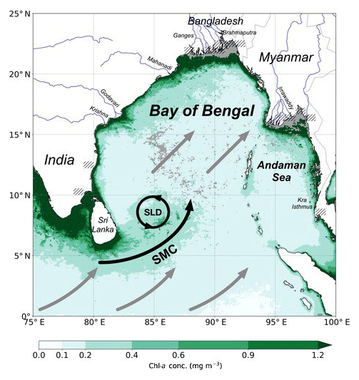
Figure 1 The Bay of Bengal (BoB) and the surrounding region of interest. The average JJAS chlorophyll-a concentration climatology measured from MODIS-Aqua at a 4 km horizontal resolution is shown. The locations of major rivers are represented as blue lines. The Sri Lanka dome (SLD) is shown as a cyclonic (anticlockwise) black circle, and the Southwest Monsoon Current (SMC) is shown using a solid black arrow. Southwesterly monsoon winds are shown using solid grey arrows. Missing chlorophyll concentration data are shown in grey. The locations of missing h₂ grid points in MC-KPP are shown using black hatching.

The South Asian monsoon is initiated when lower-tropospheric winds, transporting heat and moisture, begin to flow northward from the Equator to the Asian continent in response to increasing summer insolation and increasing land–sea thermal and pressure gradients (grey arrows in Fig. 1; Webster et al., 1998). Mid-tropospheric heating from the elevated Tibetan Plateau increases the land–sea thermal and pressure contrast, further regulating the seasonal reversal of the large-scale circulation (Li and Yanai, 1996). From June to September (June–July–August–September, JJAS), high climatological precipitation rates (> 20 mm d⁻¹), associated with the South Asian southwest monsoon, are anchored to three locations across the Indian subcontinent: the western Ghats of southwestern India, the Myanmar coast, and from Bangladesh north into the Himalayan foothills (Fig. 2f, g, h, i). Coupled ocean–atmosphere general circulation models (GCMs) have improved their representations of the seasonal variability and spatial distribution of South Asian southwest monsoon precipitation, but substantial biases remain. Lin et al. (2008) found that 12 out of 14 coupled GCMs from the Coupled Model Intercomparison Project Phase 3 (CMIP3) captured the South Asian southwest monsoon seasonal-mean precipitation rate reasonably well. However, most GCMs simulated excessive precipitation at the Equator and insufficient precipitation across the northern Bay of Bengal (BoB) and Bangladeshi region from May to October. Sperber et al. (2013) compared 25 CMIP5 models with 22 CMIP3 models. CMIP5 models have higher vertical and horizontal resolutions in the ocean and atmosphere and include additional Earth system processes compared with CMIP3 models. CMIP5 multi-model means have a better representation of precipitation rates over the western Ghats, Myanmar, and Bangladesh than CMIP3 multi-model means from June to September. However, both the CMIP5 and CMIP3 models underestimate precipitation over the BoB and India at 20^∘ N. There is also a consistent dry bias of up to 4 mm d⁻¹ over central India at 25–30^∘ N and a delay to the summer monsoon onset and peak over most of India in both CMIP5 and CMIP3 models. The significant biases from JJAS show that state-of-the-art coupled GCMs still struggle to capture the basic seasonality of summer monsoon precipitation across the BoB and the wider Indian subcontinent.

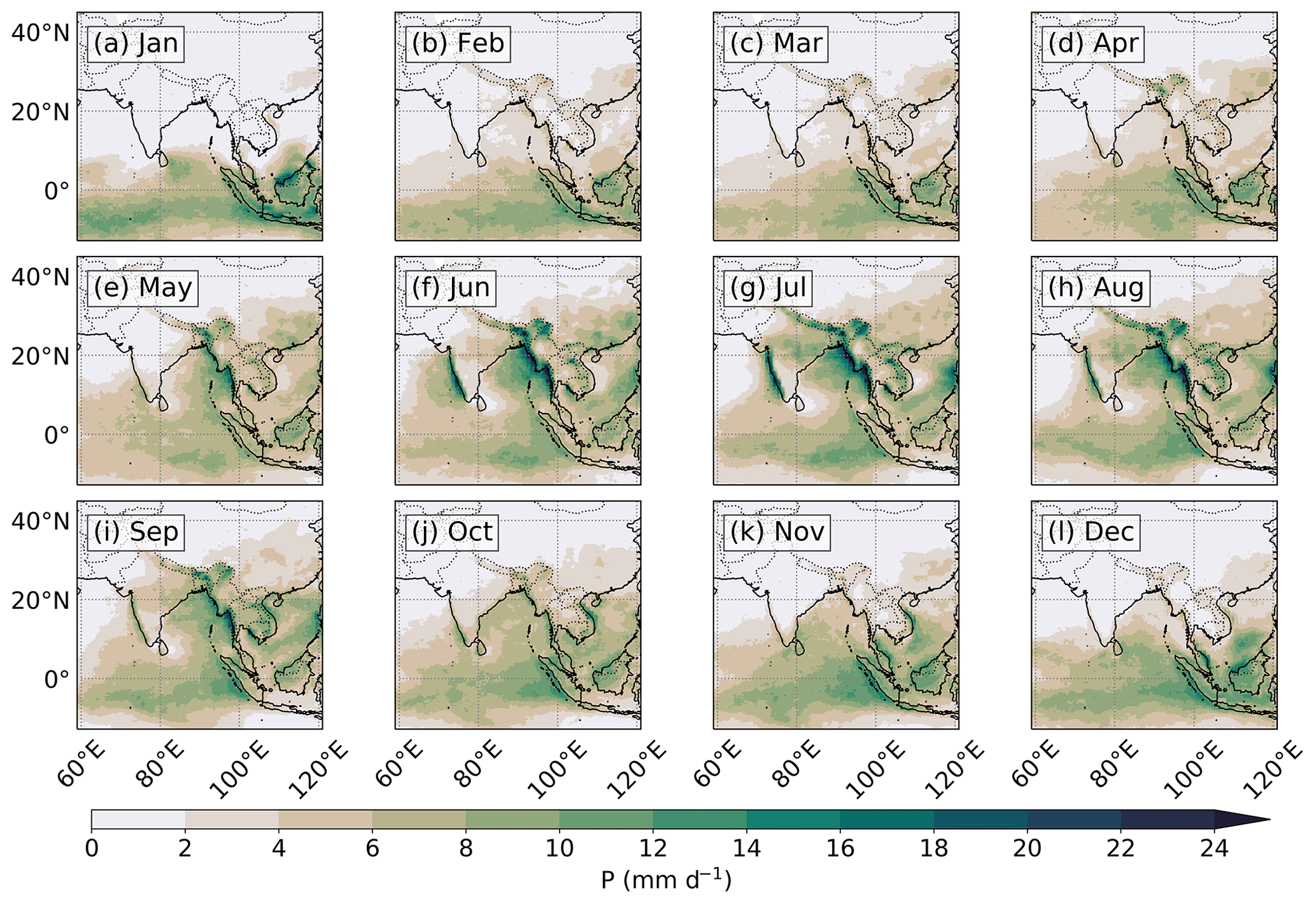
Figure 2 Monthly climatological precipitation rate measured from the Tropical Rainfall Measuring Mission (TRMM) 3B42 satellite product from January to December.

Chlorophyll significantly affects the Indian Ocean sea surface temperature (SST) and the South Asian monsoon through the absorption of sunlight (Nakamoto et al., 2000; Wetzel et al., 2006; Turner et al., 2012; Park and Kug, 2014). Nakamoto et al. (2000) used an ocean isopycnal GCM, with a two-band solar absorption scheme from Paulson and Simpson (1977), to investigate SST modulation in the Arabian Sea. Imposing a monthly climatology of chlorophyll concentrations, measured by the Coastal Zone Color Scanner (CZCS), decreased the mixed layer depth (MLD) and the solar radiation penetration depth during the inter-monsoon and increased the SST by 0.6 ^∘C. Wetzel et al. (2006) used a biogeochemistry model coupled to an ocean–atmosphere GCM to show that spring chlorophyll blooms in the western Arabian Sea increased the SST by 1 ^∘C at 20^∘ N; this led to a 3 mm d⁻¹ increase in rainfall over western India during the southwest monsoon onset. Turner et al. (2012) showed similar results when they imposed seasonally varying chlorophyll concentrations from SeaWiFS in a coupled ocean–atmosphere GCM. The spring chlorophyll blooms in the western Arabian Sea reduced the MLD biases by 50 %, increased the SST by 0.5–1.0 ^∘C, and increased rainfall by 2 mm d⁻¹ over southwestern India during the southwest monsoon onset. Park and Kug (2014) used a biogeochemistry model coupled to an ocean GCM to investigate the biological feedback on the Indian Ocean Dipole (IOD). The response to interactive biology enhanced both warming during a positive IOD (cooling in the eastern equatorial Indian Ocean) and cooling during a negative IOD (warming in the eastern equatorial Indian Ocean), thereby dampening the IOD magnitude, which could have a significant impact on the South Asian summer monsoon.

The thermal and saline surface properties of the Bay of Bengal (BoB; Fig. 1), in the northeastern Indian Ocean, are strongly forced by the monsoonal winds and large freshwater flux. In the northern BoB, the large freshwater flux from river discharge and precipitation leads to strong salinity stratification and barrier-layer formation above the thermocline and below the mixed layer (Vinayachandran et al., 2002; Jana et al., 2015; Sengupta et al., 2016). The barrier layer inhibits vertical mixing (Sprintall and Tomczak, 1992; Rao and Sivakumar, 2003) and isolates the mixed layer above from cooling by entrainment (Duncan and Han, 2009), modulating the seasonal MLD and its temperature (Girishkumar et al., 2011; Shee et al., 2019).

The BoB SST rapidly responds to variations in the net surface heat flux, which, in turn, are primarily controlled by variations in winds speed (Duncan and Han, 2009). Although the BoB SST decreases with increasing wind speed during the southwest monsoon (JJAS), the SST remains high enough (> 28 ^∘C) to sustain high precipitation rates across the Indian subcontinent, consequently strengthening the salinity stratification and further reinforcing convection across the basin (Shenoi et al., 2002). The salinity stratification is weaker in the southern BoB, allowing monsoonal winds to primarily control the upper-ocean thermal structure (Narvekar and Kumar, 2006). Hence, the southern BoB MLD and SST display larger seasonal variability compared with the northern BoB (Narvekar and Kumar, 2006).

The strong BoB salinity stratification reduces biological productivity by inhibiting the vertical transport of nutrients to the sunlit surface layers (Kumar et al., 2002; McCreary et al., 2009). Biological productivity during JJAS is also inhibited by cloud cover and by the infiltration of river sediments, which reduce the incoming solar radiation at the ocean surface and the in-water penetration depth of solar radiation respectively (Gomes et al., 2000; Kumar et al., 2010). However, in certain regions of the BoB, localized seasonal physical forcing breaks the strong stratification and increases the vertical transport of nutrients to the sunlit surface layers, increasing biological productivity. Chlorophyll concentrations in the coastal regions are high (> 1 mg m⁻³; Fig. 1), especially near large rivers such as the Ganges, Brahmaputra, Mahanadi, and Irrawaddy, due to the nutrients supplied by these rivers from June to October (Amol et al., 2019). Chlorophyll concentrations in the northern coastal region typically peak in October (Fig. 3j; Lévy et al., 2007), when river discharge and nutrients also peak (Rao and Sivakumar, 2003). High chlorophyll concentrations are then transported along the northeast coast of the BoB (Amol et al., 2019).

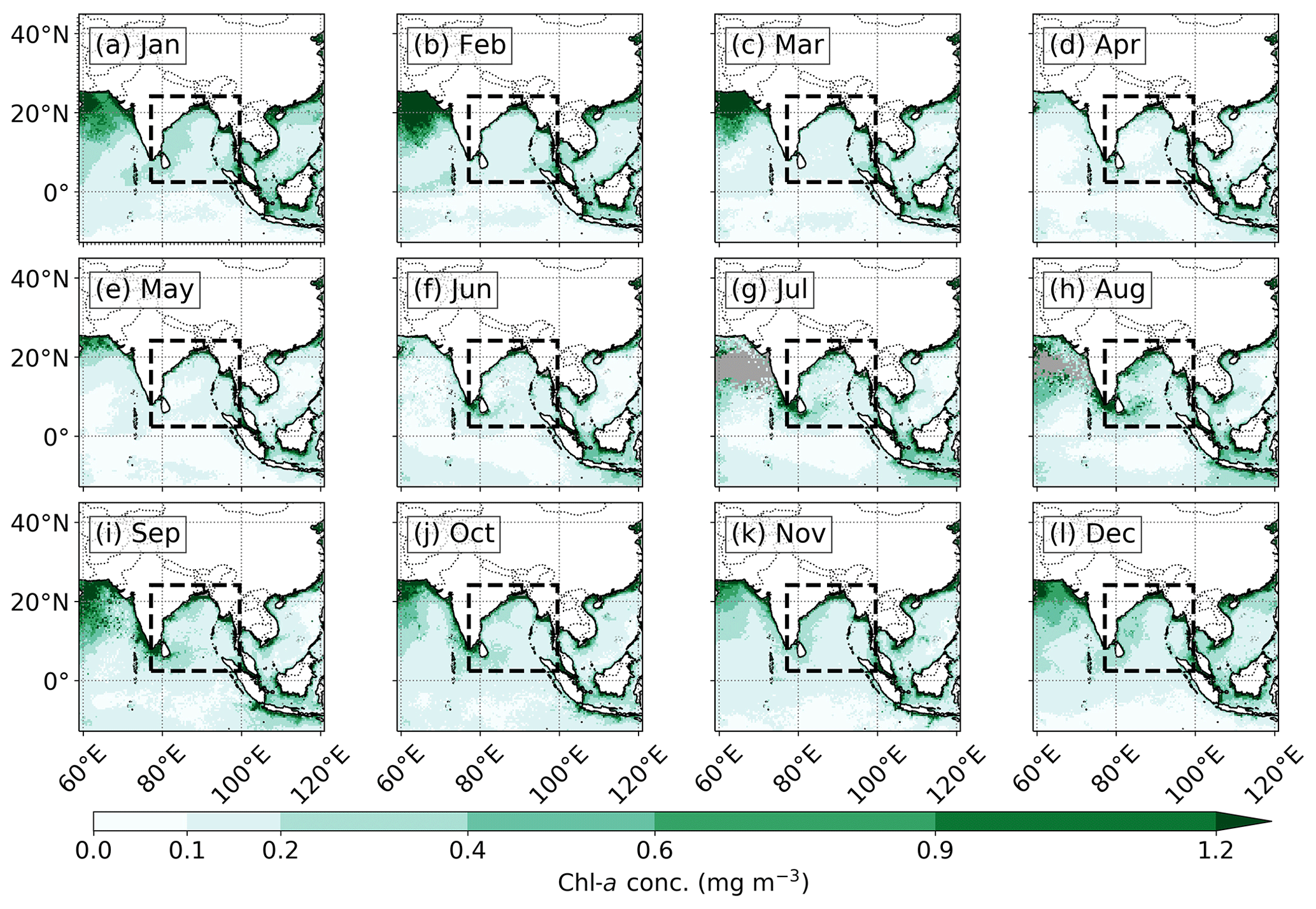
Figure 3 Monthly chlorophyll-a concentration climatology measured from MODIS-Aqua at a 4 km horizontal resolution from January to December. The BoB domain is outlined using a black dashed box (77–99.5^∘ E, 2.5–24^∘ N) that shows the location of the imposed annual cycle of chlorophyll concentrations for the perturbation simulation. Missing data are shown in grey.

In the southern BoB, strong southwesterly winds across the southernmost tip of India and Sri Lanka initiate coastal upwelling and, thus, biological productivity, leading to a maximum in the chlorophyll concentration there in August (Fig. 1; Lévy et al., 2007). The Southwest Monsoon Current (SMC), a shallow, fast current, advects these high chlorophyll concentrations to the southwestern BoB (Fig. 1; Vinayachandran et al., 2004). High chlorophyll concentrations are sustained east of Sri Lanka by the cyclonic (anticlockwise) eddy of the Sri Lanka dome (SLD), where open-ocean Ekman upwelling transfers nutrients to the near surface during JJAS (Fig. 1; Vinayachandran and Yamagata, 1998; Vinayachandran et al., 2004; Thushara et al., 2019). In the western and southwestern BoB in winter, northeasterly winds induce open-ocean Ekman upwelling, leading to increased chlorophyll concentrations peaking in December and January (Fig. 3l, a; Vinayachandran and Mathew, 2003; Lévy et al., 2007). Chlorophyll concentrations in the open BoB also show sub-seasonal and mesoscale variability. Surface chlorophyll concentrations are periodically enhanced by transient cold-core eddies and post-monsoon cyclones, where the strong salinity stratification is briefly eroded and nutrients are transported to the near surface in the western and central BoB (Vinayachandran and Mathew, 2003; Kumar et al., 2007; Patra et al., 2007).

A few studies have briefly analysed the effect of seasonally varying chlorophyll concentrations on the BoB upper-ocean dynamics and SST, whilst also speculating on how this may affect the South Asian monsoon (Murtugudde et al., 2002; Wetzel et al., 2006). Although the effect of chlorophyll on the BoB SST has been demonstrated by these previous studies, the effect of chlorophyll on monsoon rainfall remains a vital knowledge gap. Without this knowledge, missing biophysical interactions in the BoB could lead to inaccuracies in simulated air–sea interactions that are crucial for representing accurate monsoon behaviour and, thus, rainfall timing, location, and duration over the Indian subcontinent. This study analyses the direct effect of the BoB seasonally varying chlorophyll concentrations on the South Asian monsoon in an atmospheric GCM that is coupled to a mixed layer thermodynamic ocean model. A description of the experimental design, model, and observed datasets used in this study is presented in Sect. 2. Section 3 presents the results of the control and chlorophyll-perturbed model outputs. Section 4 discusses the results from the chlorophyll-perturbed experiment and provides conclusions.

2 Methods and data

2.1 MetUM-GOML

This study uses the Global Ocean Mixed Layer 3.0 configuration of the UK Met Office Unified Model (MetUM-GOML3.0), which comprises the Multi-Column K Profile Parameterization (MC-KPP version 1.2) ocean coupled to the MetUM Global Atmosphere 7.0 (Walters et al., 2019). The atmospheric and oceanic horizontal resolution is N216 (0.83^∘ longitude ×0.56^∘ latitude), which corresponds to a horizontal grid spacing of approximately 90 km. There are 85 vertical levels in the atmosphere, with approximately 50 vertical levels in the troposphere. MetUM-GOML3.0 is configured similarly to MetUM-GOML2.0 (Peatman and Klingaman, 2018) and MetUM-GOML1.0 (Hirons et al., 2015), except that the atmospheric model is updated to GA7.0 and the air–sea coupling routines are updated to couple the models via the Ocean–Atmosphere–Sea Ice–Soil (OASIS) Model Coupling Toolkit (Valcke, 2013).

MC-KPP consists of a grid of independent one-dimensional columns, with one column positioned under each atmospheric grid point at the same horizontal grid spacing as MetUM GA7.0. The ocean columns are 1000 m with 100 vertical points, with 70 points in the top 300 m; the near-surface resolution is approximately 1 m. This improves the representation of the MLD and SST, which has been shown to improve tropical convection and circulation on sub-seasonal scales when coupled to an atmospheric GCM (Bernie et al., 2005; Bernie et al., 2008; Klingaman et al., 2011). Each column is subject to surface forcing from freshwater, heat, and momentum fluxes; vertical mixing is parameterized using the KPP scheme from Large et al. (1994). The MLD is defined as the depth where the bulk Richardson number equals the critical Richardson number of 0.3 (Large et al., 1994). The coastal region in MC-KPP is represented with columns that are part ocean and part land. The surface properties for ocean and land are computed separately in MC-KPP, and the mean grid point temperatures are computed in the atmospheric model by combing the ocean and land surface temperatures from MC-KPP.

Solar radiation absorption is represented as a wavelength-dependent penetration depth, with blue wavelengths penetrating deeper than red wavelengths. The decay of solar irradiance through the water column is represented as a simple two-band double-exponential function (Paulson and Simpson, 1977):

$$\begin{array}{}\text{(1)}& {\displaystyle \frac{I\left(z\right)}{I_{\mathrm{0}}}}=R{e}^{-\frac{z}{h_{\mathrm{2}}}}+(\mathrm{1}-R)e^{-\frac{z}{h_{\mathrm{2}}}},\end{array}$$

where I(z) is the solar irradiance at depth z, I₀ is the solar irradiance at the ocean surface, R is the ratio of red light to the total visible spectrum, and h₁ and h₂ are the scale depths of red and blue light respectively. The scale depth, or e-folding depth, is defined as the depth where solar irradiance is approximately 63 % less than its surface value ($\mathrm{1}-e^{-\mathrm{1}})$. Paulson and Simpson (1977) determined the optical parameters based on each of the five Jerlov water types that categorize open-ocean turbidity (Jerlov, 1968). Water type IB represents the average open-ocean turbidity, where chlorophyll concentrations are ∼0.1 mg m⁻³ (Morel, 1988); h₁ and h₂ are 1 m and 17 m respectively. Increasing the upper-ocean turbidity to water type III, where chlorophyll concentrations exceed 1.5–2.0 mg m⁻³ (Morel, 1988), yields h₁ and h₂ of 1.4 and 7.9 m respectively. The scale depth for red light (h₁∼1–1.4 m) for all water types is much less than the typical MLD (> 10 m). Hence, all red light is absorbed at the top of the mixed layer. However, the scale depth for blue light (h₂∼8–17 m) is comparable to the typical MLD; a significant fraction of blue light will penetrate below the mixed layer. Hence, the reduction of h₂ with increasing turbidity controls the radiant heating of the mixed layer and, thus, the SST (Zaneveld et al., 1981; Lewis et al., 1990; Morel and Antoine, 1994).

MC-KPP uses the Paulson and Simpson (1977) scheme (Eq. 1) for the absorption of red and blue light with depth through the upper ocean. In this study, a h₂ of 17 m from Jerlov water type IB is used to represent the global average solar penetration depth in MC-KPP. Chlorophyll and biogeochemical processes are not included. The effect of chlorophyll on the ocean is modelled by specifying h₂.

MC-KPP does not represent horizontal or vertical advection. The ocean temperature and salinity correction method of Hirons et al. (2015) is used to constrain the MC-KPP mean state to account for missing advection and biases in atmospheric surface fluxes. The method uses a separate 10-year MetUM-GOML relaxation simulation in which temperature and salinity are relaxed with a 15 d timescale to an observed seasonal cycle, here the 1980–2009 climatology of Smith and Murphy (2007). A relaxation timescale of 15 d is optimal to produce temperature and salinity tendency terms that minimize biases in the free-running simulations (Hirons et al., 2015). A mean seasonal cycle of daily temperature and salinity tendencies that is computed from this relaxation simulation is applied to the 30-year chlorophyll perturbation simulations. The spin-up time is small (1 year), as the ocean is adjusted to a mean state after the relaxation simulation. The absence of ocean dynamics means that MetUM-GOML does not represent coupled modes of variability (e.g. ENSO or IOD) which rely on a dynamical ocean (Hirons et al., 2015). The benefit of not representing these modes of variability is that the signal from the chlorophyll perturbation experiment will not be obscured by the “noise” of these interannual climate variations. The absence of full ocean dynamics also reduces the computational cost and allows the model to be used for climate-length coupled simulations with shorter spin-up periods (Hirons et al., 2015).

We directly impose a seasonally varying h₂ value (representative of chlorophyll concentration) to selected columns within the BoB region, whilst the global ocean outside the BoB region has a constant h₂ value. This set-up enables us to investigate the direct impact of chlorophyll on BoB surface ocean properties, atmospheric surface fluxes, and the regional climate. Furthermore, the absence of biological and physical feedbacks on chlorophyll development means that a consistent seasonally varying h₂ value is directly imposed on columns within the BoB throughout the simulation.

2.2 Chlorophyll-a data

To produce a temporally and spatially varying field of h₂ for MC-KPP, a monthly climatology of chlorophyll-a concentration, measured from the Moderate Resolution Imaging Spectroradiometer (MODIS) on the Aqua satellite, was used. MODIS-Aqua chlorophyll-a concentration (available from NASA's Ocean Color database; https://oceancolor.gsfc.nasa.gov, last access: 9 August 2020) is available as a 17-year climatology (2002–2018) at a spatial resolution of 4 km. The backscattered solar radiation from the ocean surface (water-leaving radiance) in nine spectral bands between 412 and 869 nm measured by MODIS-Aqua were used to calculate the chlorophyll-a concentration (Hu et al., 2012b). Chlorophyll-a concentration retrievals below 0.25 mg m⁻³ were calculated using the “color index” (CI) three-band reflectance algorithm (Hu et al., 2012b). Chlorophyll-a retrievals above 0.3 mg m⁻³ were calculated using the “ocean color 3” (OC3) algorithm, which is a fourth-degree polynomial relating three wavelengths of water-leaving radiance (433, 490 and 550 nm) to the chlorophyll-a concentration (O'Reilly et al., 2000). Chlorophyll-a retrievals from 0.25 to 0.3 mg m⁻³ were calculated by merging the CI and OC3 algorithms to create the “ocean color index” (OCI) algorithm (Wang and Son, 2016; Hu et al., 2019). Chlorophyll-a concentration retrievals above 5 mg m⁻³ reduce the effectiveness of the OC3 algorithm (Morel et al., 2007). Organic and terrestrial material, introduced by rivers or mixed by tidal currents in coastal regions, change the scattering of visible light, affecting the water-leaving radiances (Boss et al., 2009) and leading to an overestimate of the chlorophyll-a concentration (Morel et al., 2007). Hence, remotely sensed chlorophyll-a concentrations were not determined in the eutrophic coastal regions of the Ganges and Irrawaddy river deltas due to the large amount of suspended organic and terrestrial material (grey shading in Fig. 1; Tilstone et al., 2011). MODIS sensor degradation on the Aqua satellite has been small (Franz et al., 2008), and all ocean colour products have since been corrected and improved after cross-calibration with the SeaWiFS climatology (Meister and Franz, 2014). Chlorophyll a will henceforth be referred to as “chlorophyll” for convenience.

2.3 Experiment set-up

To investigate the impact of the seasonal and spatial variability of chlorophyll-induced heating in the BoB, two 30-year simulations with differing prescribed h₂ (representative of chlorophyll concentrations) were completed: a control run using h₂=17 m globally and a perturbation run using an annual cycle of h₂ at a daily resolution for the BoB region (defined below) and h₂=17 m over the rest of the global ocean. In both simulations, R and h₁ were kept constant, at 0.67 and 1.0 m respectively, which are values representative of water type IB. The first year of both simulations was discarded due to spin up; the analysis was carried out on the remaining 29 years.

The control simulation used an effective constant global chlorophyll concentration of ∼0.15 mg m⁻³, which corresponds to h₂= 17 m (Jerlov water type IB; Morel, 1988). Some previous studies have used control simulations with zero chlorophyll concentrations to see the full impact of chlorophyll on physical and dynamical processes (e.g. Gnanadesikan and Anderson, 2009), whereas other studies have used constant scale depths determined from parameterizations of the lowest chlorophyll concentrations encountered (e.g. Shell et al., 2003; Turner et al., 2012). Satellite observations show that the global average chlorophyll concentration for oceans deeper than 1 km is 0.19 mg m⁻³ (Wang et al., 2005), similar to the value in our control simulation.

For the perturbation simulation, the BoB region was defined as the area from 77 to 99.5^∘ E and from 2.5 to 24^∘ N (black dashed box in Fig. 3). The region extends far enough south and west to incorporate the high surface chlorophyll around the southernmost tip of India and Sri Lanka, but it excludes the relatively low near-equatorial surface chlorophyll concentrations (Fig. 3f, g, h, i, j). The Kra Isthmus and Myanmar to the east and India and Bangladesh to the north and west form a natural boundary to the defined BoB region (Fig. 1). An annual cycle of daily chlorophyll concentration for MetUM-GOML was derived by linearly interpolating the monthly climatology to daily values and then re-gridding from the resolutions of the observations (4 km) to MetUM-GOML (∼90 km).

Satellite-derived chlorophyll concentrations were converted to h₂ using a fifth-order polynomial parameterization from Morel and Antoine (1994) (Fig. 4a, b, c). This high-order polynomial relationship relates blue light from a two-band solar absorption scheme to surface chlorophyll concentrations that are assumed to have a Gaussian vertical profile in the upper ocean. The relationship shows the scale depth varying as a power law function of the surface chlorophyll concentration with the largest variability in the scale depth (> 18 m) at the lowest concentrations (< 0.1 mg m⁻³).

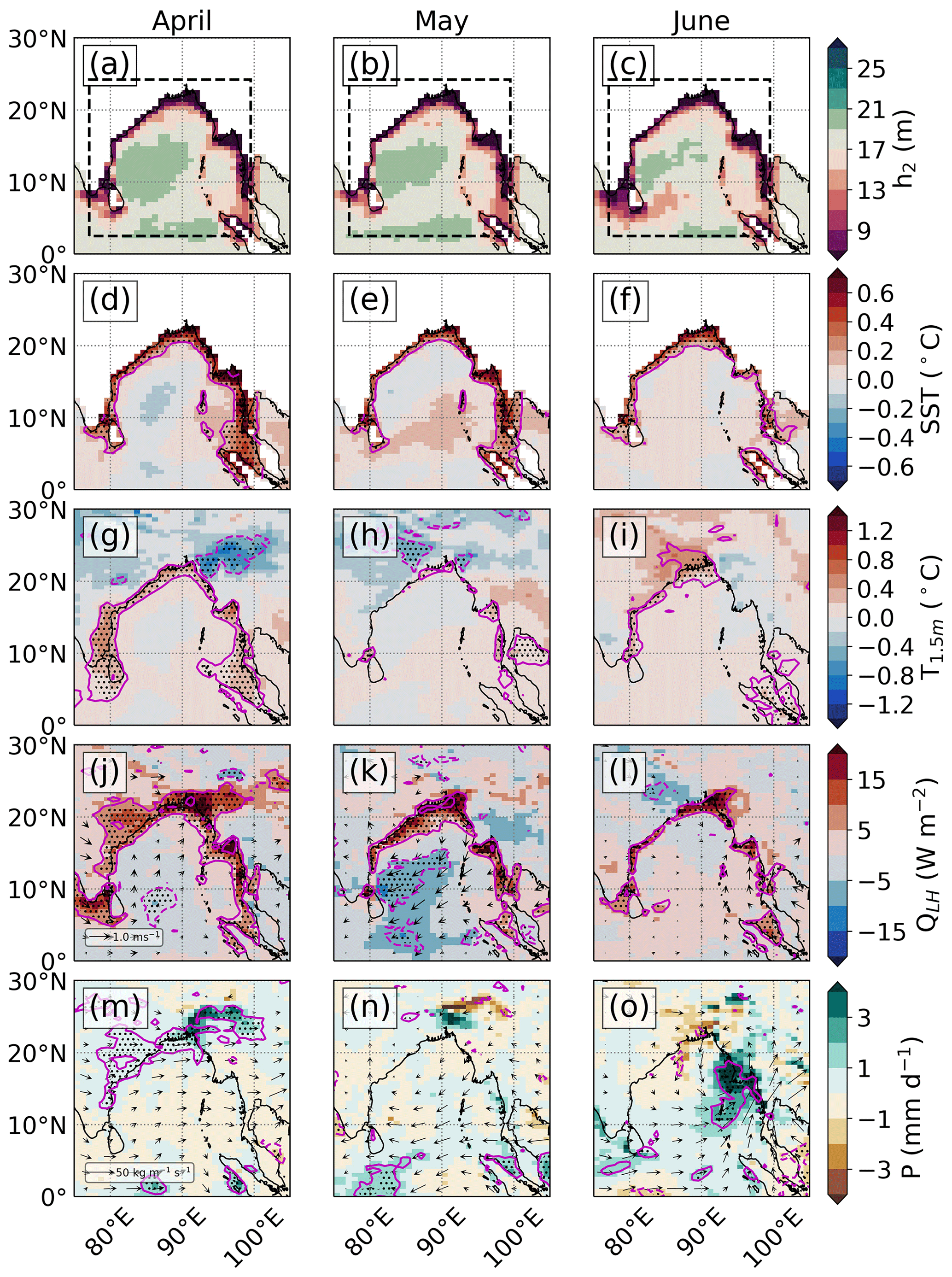
Figure 4 Monsoon onset season (April to June). (a–c) Monthly average h₂ (m) in the perturbation run. Monthly 29-year average difference (perturbation minus control) of (d–f) the SST (^∘C), (g–i) the 1.5 m air temperature (^∘C), (j–l) the upward latent heat flux (W m⁻²) and 10 m wind velocity (m s⁻¹), and (m–o) the precipitation rate (mm d⁻¹). The magenta line shows the 10 % significance level, and the black stippling shows the 5 % significance level.

Missing h₂ data were common in regions such as the Ganges River delta due to undetermined remotely sensed chlorophyll concentrations from highly turbid coastal waters. Missing h₂ data in this delta extend further out onto the continental shelf during JJAS as floodwaters drain into the BoB transporting finer silt and clay further offshore (Kuehl et al., 1997). The missing h₂ data were typically associated with regions where the land fraction was less than one, which includes the narrow Kra Isthmus and the low-lying land of the Ganges River delta (black hatching in Fig. 1). A minimum of two h₂ values from two neighbouring data points were required to find an average h₂ value to fill in the missing data point. To avoid sharp gradients at the boundary of the BoB domain, the seasonally varying h₂ values within the BoB domain were smoothly transitioned (linearly) to the constant h₂= 17 m outside the BoB domain, over a buffer region of three grid points.

Vertically integrated moisture fluxes (VIMF) were used to evaluate the water vapour transport sourced from the chlorophyll-forced BoB to the surrounding Indian subcontinent. The VIMF was calculated as follows:

$$\begin{array}{}\text{(2)}& \mathrm{VIMF}={\displaystyle \frac{\mathrm{1}}{g}}\int \mathit{u}q\mathrm{d}p,\end{array}$$

where u is the horizontal wind velocity, q is the specific humidity, g is the acceleration due to gravity, p is pressure, and the integration was between 1000 and 100 hPa. Note that uq was output directly by the model as monthly mean values. VIMF divergence was used to evaluate the precipitation rate changes that are due to changes in water vapour divergence. The VIMF divergence was calculated as follows:

$$\begin{array}{}\text{(3)}& \mathrm{VIMFD}={\displaystyle \frac{\mathrm{1}}{g}}\int {\displaystyle \frac{\partial \mathit{u}q}{\partial x}}+{\displaystyle \frac{\partial \mathit{v}q}{\partial y}}\mathrm{d}p,\end{array}$$

where the integration was between 1000 and 100 hPa.

The observed monthly 18-year (1998–2015) climatological precipitation rate measured from the Tropical Rainfall Measuring Mission (TRMM) 3B42 satellite product (Huffman et al., 2007) was used to diagnose the bias in the model precipitation rate. An area-weighted re-gridding scheme was used to reduce the 0.25^∘ horizontal resolution of the observed monthly climatological precipitation rate to match the horizontal resolution of MetUM-GOML.

3 Results

3.1 Southwest monsoon onset (April to June)

The BoB surface ocean responds to the imposed annual cycle of h₂ in the perturbation run during the onset of the southwest monsoon. In the central BoB, values of h₂ increase above the global constant of 17 m, as observed surface chlorophyll concentrations are low during the southwest monsoon onset (Fig. 4a, b, c). Along the northern BoB coast, values of h₂ are as low as 5 m, as observed surface chlorophyll concentrations in coastal areas are higher than those in the central BoB (Fig. 4a, b, c). During May and June, the values of h₂ decrease and mixed layer solar absorption increases in the northwestern BoB, as observed high coastal chlorophyll concentrations extend oceanward across the continental shelf (Fig. 4b, c). In the southwestern BoB, the imposed h₂ decreases to 14 m in May and June, as the strengthening SMC advects high chlorophyll concentrations from the southern coast of India and Sri Lanka (Fig. 4b, c).

The imposed annual cycle of h₂ directly affects coastal SST. During April, the increase in solar absorption by chlorophyll along the northern and western coastal regions significantly (at 5 % level) increases the monthly average SST by 0.5 ^∘C (Fig. 4d). Correspondingly, the monthly average 1.5 m air temperature increases by 0.5 ^∘C in the perturbation run (Fig. 4g). The strengthening alongshore wind over the warmer western coast results in a large increase of 20 W m⁻² in the upward latent heat flux (Fig. 4j). This increase in atmospheric moisture leads to an anomaly of 30 kg m⁻¹ s⁻¹ in the VIMF (Fig. 5a) that is in the same direction as the mean VIMF in the control run (Fig. 6a). The increase in the VIMF converges over northeast India and Bangladesh as shown by the negative VIMF divergence (Fig. 5a), supplying the extra moisture needed for the 2 mm d⁻¹ increase in the precipitation rate (significant at the 5 % level; Fig. 4m).

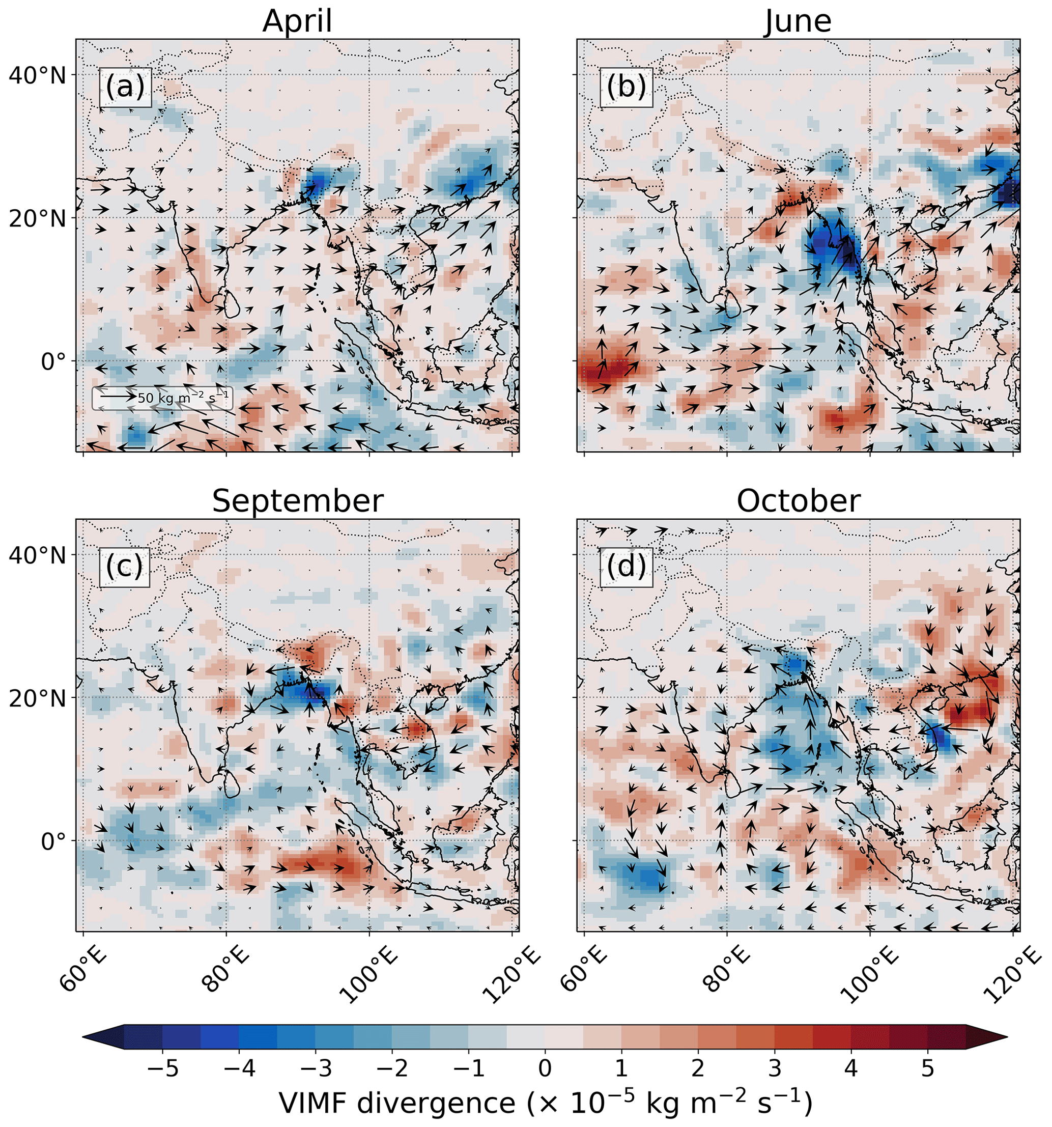
Figure 5 Monthly 29-year average difference (perturbation minus control) of VIMF (vector arrows) and VIMF divergence (shaded) for (a) April, (b) June, (c) September, and (d) October.

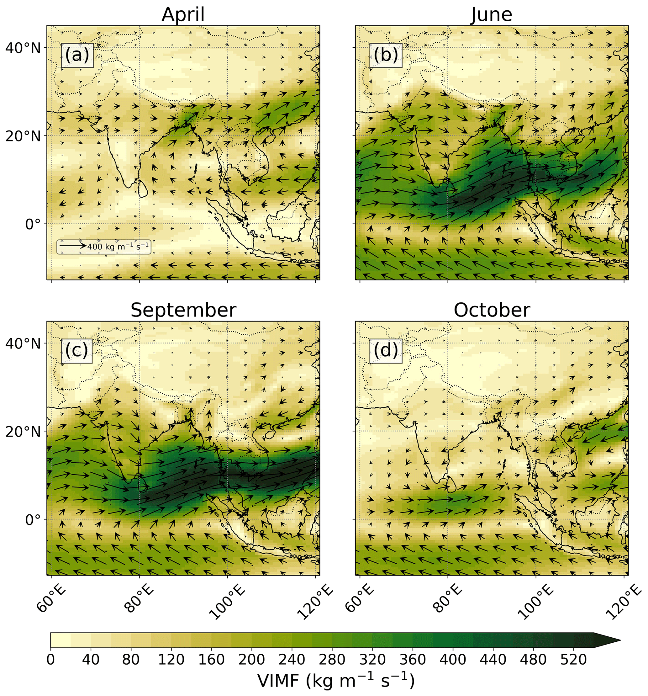
Figure 6 Monthly 29-year average VIMF from the control run for (a) April, (b) June, (c) September, and (d) October.

The increase in solar absorption in the mixed layer due to high chlorophyll concentrations persists during May and June along the coasts (Fig. 4b, c). Low h₂ along the northern and western BoB coastal regions acts to increase the monthly average SST by 0.5 ^∘C (Fig. 4e, f). The upward latent heat flux increases (Fig. 4k, l) due to an increase in the specific humidity at the surface, which is associated with the higher SST. Thus, this increase in SST is offset by the negative feedback from the latent heat flux increase.

In June, the precipitation rate over the Myanmar coast increases by 3 mm d⁻¹ (significant at the 5 % level; Fig. 4o). The monthly average 1.5 m air temperature increases by 0.4^∘C (Fig. 4i), which is caused by an increase in the SST (Fig. 4f) where h₂ along the western BoB is low (Fig. 4c). The upward latent heat flux increases by 10 W m⁻² (Fig. 4l) and the VIMF increases by 20 kg m⁻¹ s⁻¹ (Fig. 5b) in addition to a strengthening southwesterly moisture transport during the southwest monsoon onset (Fig. 6b). The enhanced convergence of the VIMF over the Myanmar coast (Fig. 5b) supplies the moisture for the increase in the precipitation rate (Fig. 4o). Thus, we have demonstrated that high coastal chlorophyll concentrations perturb the absorption of solar radiation that increases air temperature and SST, which, in turn, significantly increases spring inter-monsoon precipitation rates in the northern and eastern BoB.

3.2 Southwest monsoon (July to October)

The values of h₂ continue to decrease in the BoB open ocean into July and August (Fig. 7a, b), as high chlorophyll concentrations off the continental shelf and SMC encroach further into the central BoB. The lowest monthly average h₂ in the SMC region and the central BoB occurs in August with a value of 12 and 15 m respectively (Fig. 7b). During September and October, the SMC weakens and the observed high chlorophyll concentrations retreat back to the coast, increasing the average h₂ in the SMC region and the central BoB to around 16 m (Fig. 7c, d). Meanwhile, along the northwestern BoB during October, the monthly average h₂ decreases to 13 m, as observed high chlorophyll concentrations retreat back onto the continental shelf (Fig. 7d).

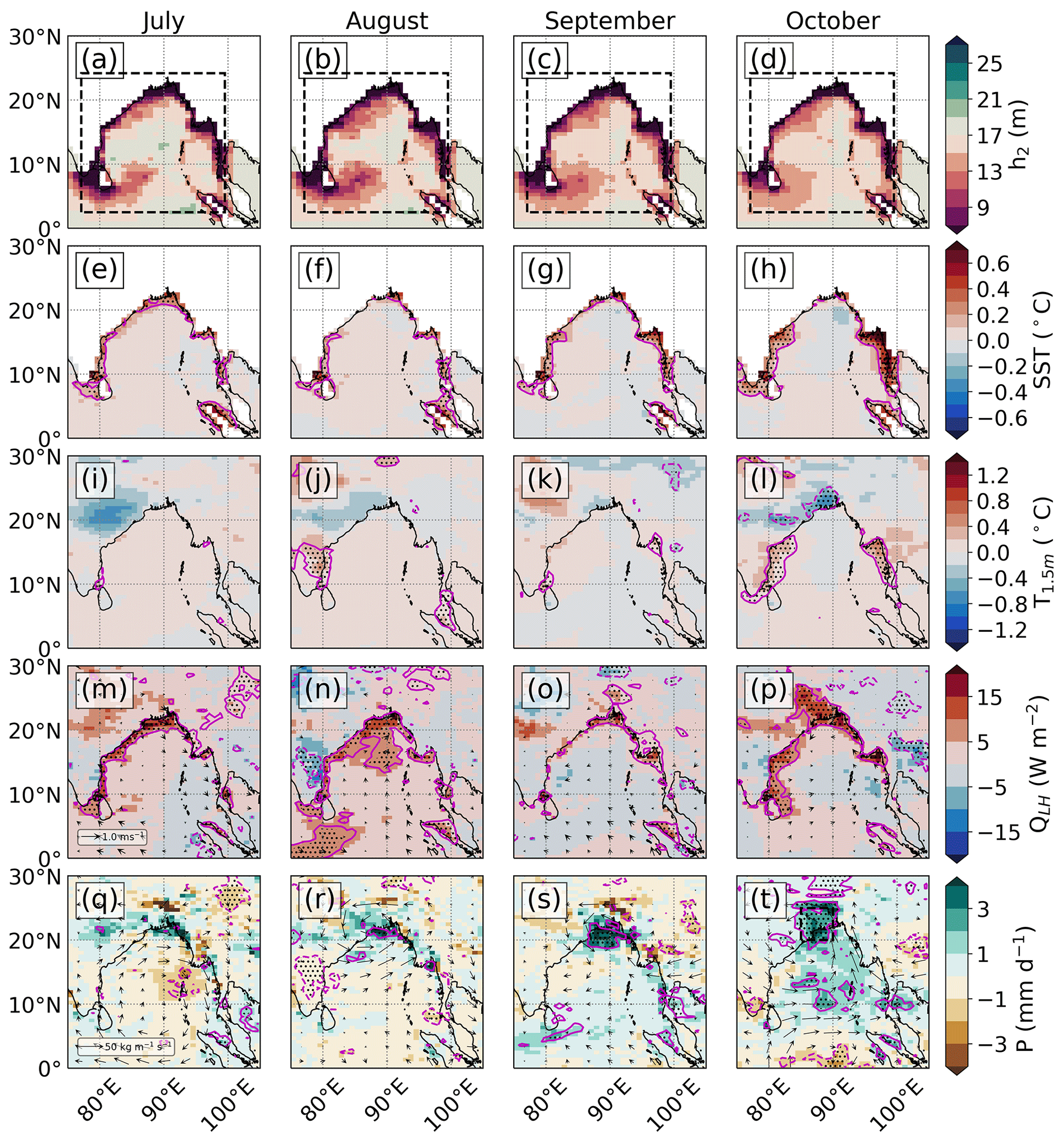
Figure 7 As in Fig. 4 but for the southwest monsoon season (July to October). Panel (t) displays the location of the monthly 29-year area-weighted average precipitation rate in Fig. 9 as a black dashed box (85–90^∘ E, 20–25^∘ N).

BoB surface ocean and regional climate respond to the above changes in h₂ during JJAS. Higher coastal SSTs (significant at the 10 % level) are co-located with the high coastal chlorophyll concentrations, whereas open-ocean SST is largely unchanged by BoB chlorophyll forcing (Fig. 7e, f, g). In July, an increase in the SST and a slight increase in the alongshore wind speed over the western BoB increase the upward latent heat flux (Fig. 7m), but this does not significantly change the precipitation rate (Fig. 7q). In August, a further increase in the alongshore wind speed increases the magnitude and spatial extent of the upward latent heat flux across the northern BoB (Fig. 7n). During September, an increase in wind speeds over the northern Myanmar coast increases surface ocean evaporation (Fig. 7o). The VIMF increases in magnitude and remains approximately in the same direction as the mean VIMF in the control run (Figs. 5c, 6c). The negative VIMF divergence over the northern Myanmar and Bangladeshi coast in the perturbation run (Fig. 5c) supplies moisture for the increase in the precipitation rate in this region (significant at the 5 % level; Fig. 7s).

By October the combined atmospheric moisture sourced from the warmer western BoB and Andaman Sea leads to an increase in the precipitation rate of up to 3 mm d⁻¹ over western Bangladesh and northeastern India (significant at the 5 % level; Fig. 7t). The spatial extent of the increased precipitation rate is considerably larger than in previous months, extending further west over the Indo-Gangetic Plain and encompassing megacities such as Kolkata and Dhaka. An area-weighted 29-year monthly average precipitation rate over western Bangladesh and northeastern India (20–25^∘ N, 85–90^∘ E; black dashed box in Fig. 7t) shows a rainfall maximum in August in both simulations (Fig. 8a). The precipitation rate differences gradually increase from July to August and peak in at 2 mm d⁻¹ October (Fig. 8b). Alongshore winds over the warmer Kra Isthmus and the coast of Myanmar further increase atmospheric moisture transport to the northern BoB (Fig. 6d). The upward latent heat flux increases by 13 W m⁻² (Fig. 7p) and the VIMF increases by 30 kg m⁻¹ s⁻¹ over the coast of Myanmar (Fig. 5d). The negative VIMF divergence over western Bangladesh and northeastern India supplies moisture for the increase in the precipitation rates in this region (Fig. 5d). As in the spring inter-monsoon, the increase in the precipitation rate during the autumn inter-monsoon in the northern BoB is primarily attributed to high coastal chlorophyll concentrations and an increased SST extending from the Andaman Sea to the Ganges River delta along the chlorophyll-perturbed BoB coastal region.

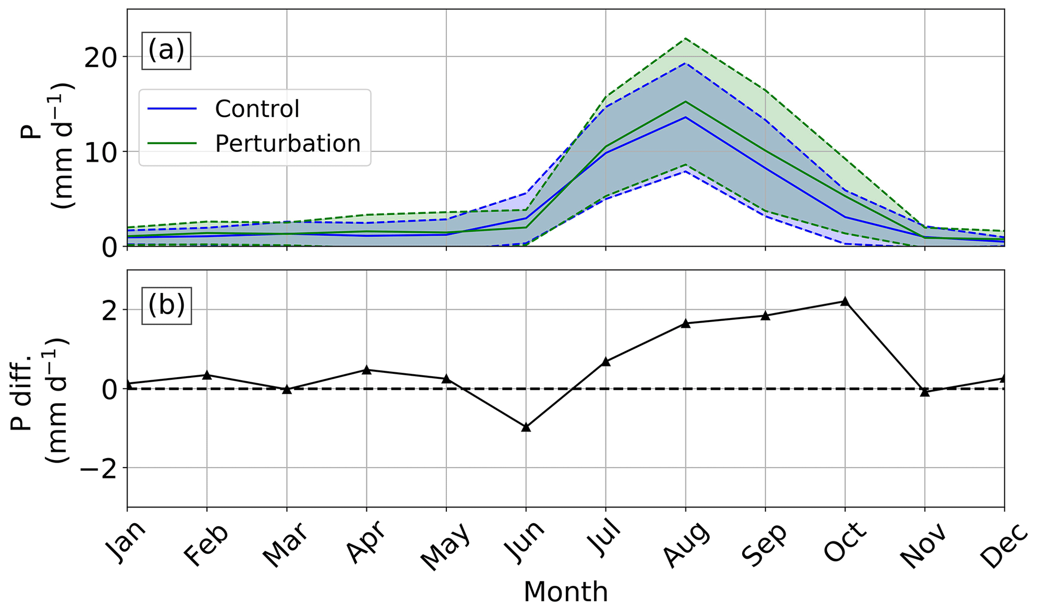
Figure 8 (a) Monthly 29-year area-weighted average precipitation rate for the control run (blue solid line) and the perturbation run (green solid line) for the 85–90^∘ E, 20–25^∘ N region. The shaded region between the dashed lines shows the 1 standard deviation variability. (b) The difference in the monthly 29-year area-weighted average precipitation rate between the control and perturbation run.

The enhanced convective activity over western Bangladesh and northeastern India during October is associated with an increase the vertical wind velocity at the 500 hPa pressure level (Fig. 9a). At the 200 hPa pressure level, enhanced westerly winds converge over eastern China (Fig. 9b), which leads to increased subsidence (Fig. 9a). This subsidence reduces precipitation and increases the surface temperature over eastern China (significant at the 5 % level; Fig. 9c, d). This indirect remote response resembles the effect of the “Silk Road” pattern; a stationary Eurasian–Pacific Rossby wave train that occurs during the Northern Hemisphere summer and produces significant air temperature and rainfall anomalies in East Asia (Ding and Wang, 2005).

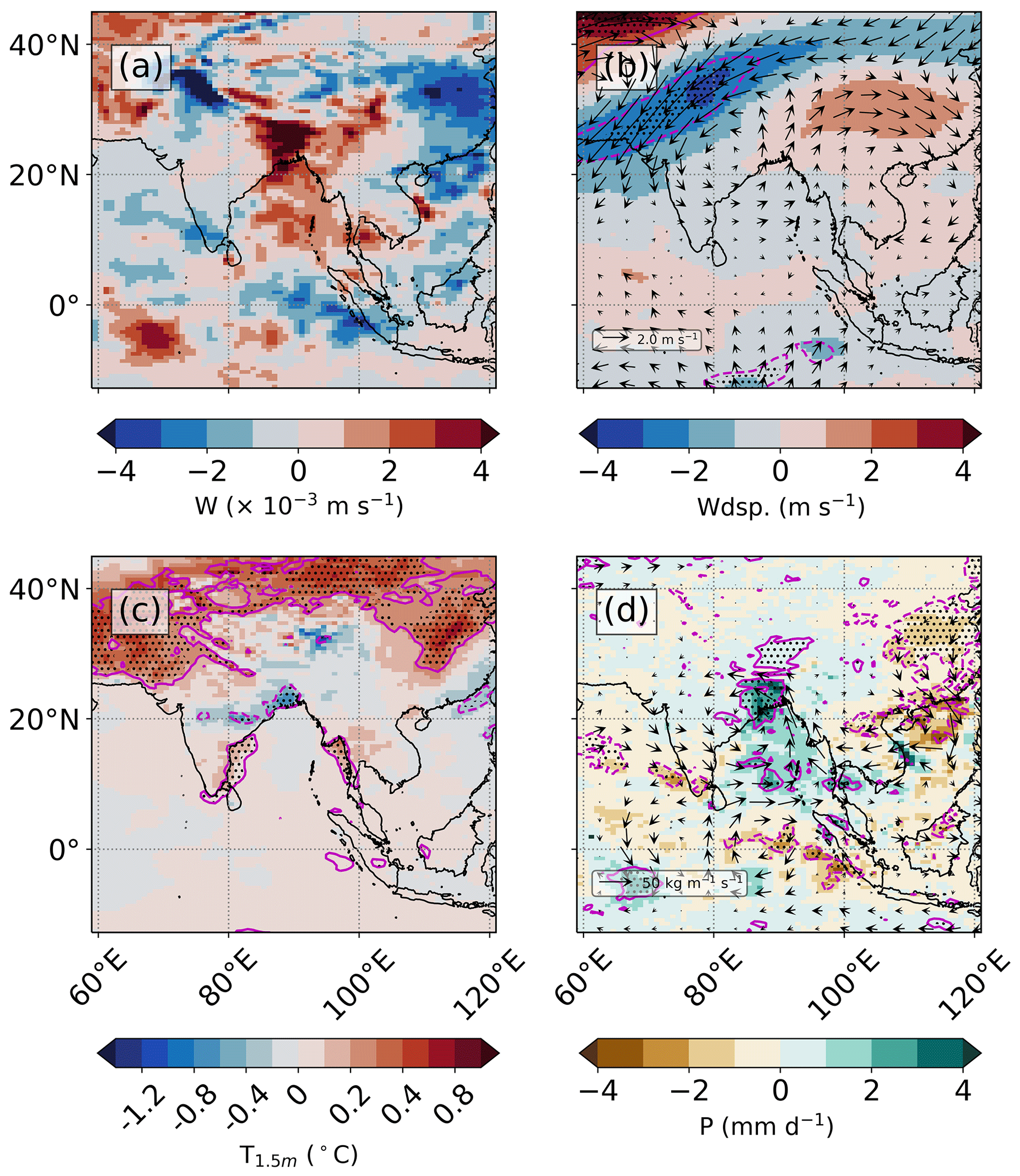
Figure 9 October 29-year average difference (perturbation minus control) of (a) the 500 hPa vertical velocity (m s⁻¹), (b) the 200 hPa horizontal vector wind (m s⁻¹), (c) the 1.5 m air temperature (^∘C), and (d) the precipitation rate (mm d⁻¹) and VIMF (kg m⁻¹ s⁻¹). The magenta line shows the 10 % significance level, and the black stippling shows the 5 % significance level.

3.3 Mixed layer radiant heating and SST modulation

The hypothesized direct link between a change in h₂ and a resultant change in SST is examined in more detail in this subsection. The radiant heating rate of the mixed layer and the resultant change in SST depend not only on h₂ but also on changes in the surface flux of shortwave radiation, which is dependent on cloud cover, and changes in the depth of the mixed layer. Here, we assess which of these three factors is primarily responsible for the changes in the radiant heating rate of the mixed layer.

We assume that the red-light radiative flux is absorbed within approximately the top 1 m and entirely within the mixed layer, and only the blue-light radiative flux can partially penetrate below the mixed layer. The radiant heating rate of the mixed layer is calculated as follows:

$$\begin{array}{}\text{(4)}& \mathrm{RHR}={\left.{\displaystyle \frac{\mathrm{d}T}{\mathrm{d}t}}\right|}_Q={\displaystyle \frac{Q_{\mathrm{sw}}\left(\mathrm{0}\right)-(\mathrm{1}-R)Q_{\mathrm{sw}}\left(\mathrm{0}\right)e^{-\frac{\mathrm{H}}{h_{\mathrm{2}}}}}{\mathit{\rho }{c}_{\mathrm{p}}\mathrm{H}}},\end{array}$$

where T is the temperature of the mixed layer, t is time, Q_sw(0) is the monthly 29-year average downward shortwave radiation flux incident at the ocean surface, ρ=1025 kg m⁻³ is the density of the mixed layer, c_p=3850 J kg⁻¹ K⁻¹ is the specific heat capacity of sea water, R=0.67 is the ratio of red light to total visible light for Jerlov water type IB, H is the monthly 29-year average MLD, and h₂ is the monthly average h₂ that was imposed in the control and perturbation run.

Within the BoB, the largest imposed change in h₂ is 13 m. Assuming that the other variables remain constant, a change in h₂ of 13 m changes radiant heating rates by 0.4 ^∘C per month. The largest model change in downward shortwave radiation is 14 W m⁻², which changes radiant heating rates by 0.3 ^∘C per month, comparable to the change from h₂ variations. The largest model MLD change is 3 m, which changes radiant heating rates by 0.4 ^∘C per month, also comparable to the change from h₂ variations.

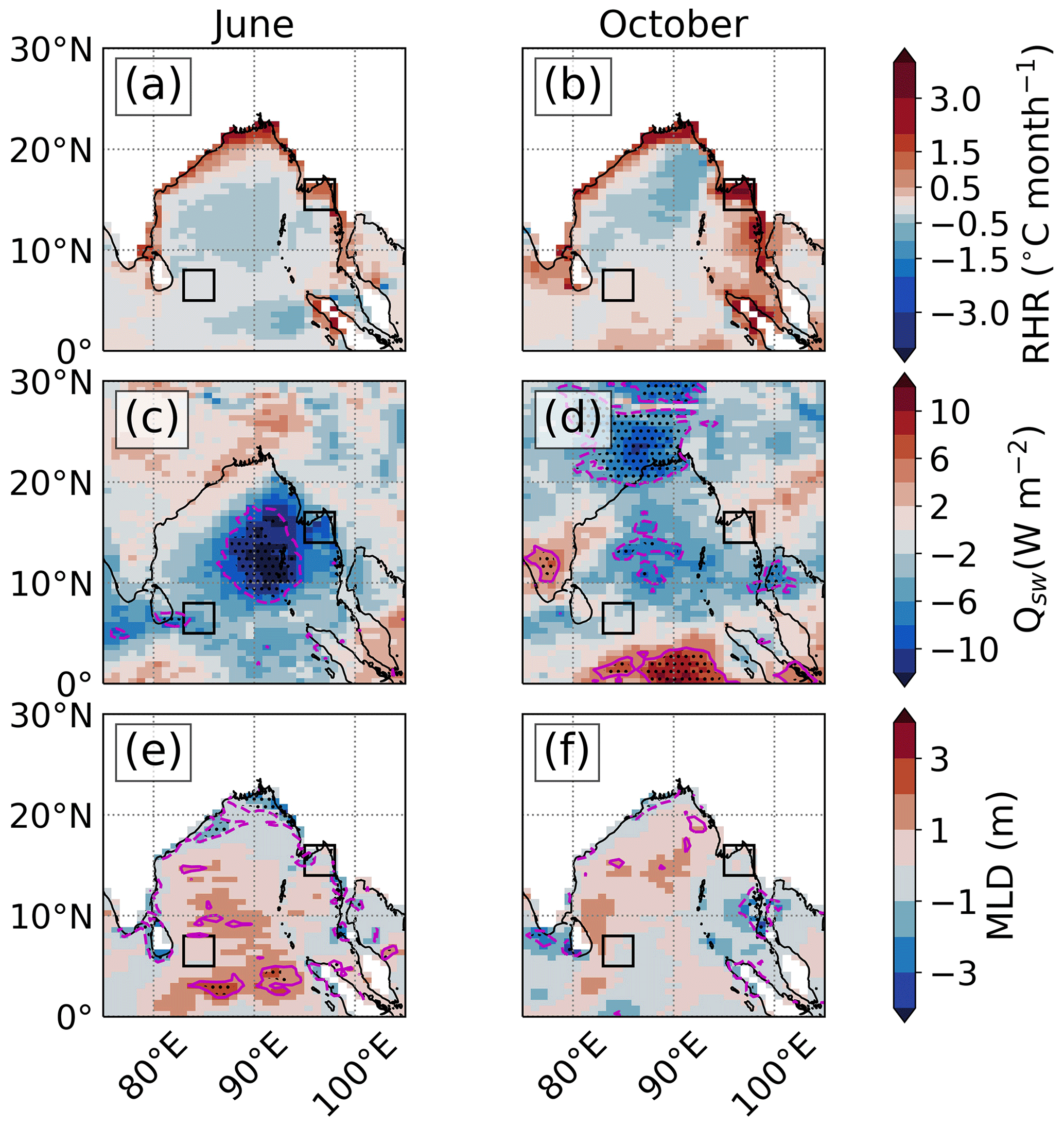
Figure 10 Monthly 29-year average difference (perturbation minus control) of (a, b) the radiant heating rate (^∘C per month), (c, d) the downward shortwave radiation flux (W m⁻²), and (e, f) the mixed layer depth (m) for June and October. The black boxes show the location of the open-ocean region of the SMC (southwestern BoB; 83–86^∘ E, 5–8^∘ N) and the coastal region of the Irrawaddy Delta (northeastern BoB; 95–98^∘ E, 14–17^∘ N). The magenta line shows the 10 % significance level, and the black stippling shows the 5 % significance level.

We compare the mixed layer radiant heating rates of the control and perturbation runs during June and October (Fig. 10a, b). We focus on two regions: the open-ocean region of the SMC (83–86^∘ E, 5–8^∘ N; black boxes in Fig. 10) and the coastal region of the Irrawaddy Delta (95–98^∘ E, 14–17^∘ N; black boxes in Fig. 10). These two regions are an important source of heat and moisture for the June and October precipitation rate perturbations and display distinctive chlorophyll regimes. The SMC is an open-ocean region that displays large seasonal changes in h₂, whereas the Irrawaddy Delta is a coastal region that displays continuously low h₂. In June and October, coastal regions have the highest radiant heating rate difference between the control and perturbation runs (Fig. 10a, b). In June, the area-weighted mean radiant heating rate in the coastal region of the Irrawaddy Delta increases by 0.4 ^∘C per month in the perturbation run (Fig. 10a). A h₂ decrease of 9 m has the largest contribution to the radiant heating rate increase of 0.7 ^∘C per month (Fig. 11a) compared with an MLD decrease of 0.2 m (Fig. 10e), which contributes to less than 0.1 ^∘C per month (Fig. 11e). A decrease in the downward shortwave radiation flux of 8 W m⁻² (Fig. 10c), associated with an increase in monsoon cloud cover, cools the region by 0.3 ^∘C per month (Fig. 11c). In October, the radiant heating rate difference in the Irrawaddy Delta increases by 1.5 ^∘C per month in the perturbation run (Fig. 10b). The radiant heating rate difference is larger than June because of an increase in the monthly average downward shortwave radiation flux and a shallower MLD in both the control and perturbation runs. A decrease in h₂ of 9 m has the largest contribution to the radiant heating rate increase of 1.4 ^∘C per month (Fig. 11a), whereas a decrease in the MLD of 0.1 m (Fig. 10f) and an increase in downward shortwave radiation flux of 1 W m⁻² (Fig. 10d) only contribute to less than 0.1 ^∘C per month of the increase in radiant heating rate respectively (Fig. 11d, f). The changes in h₂ are more influential on the mixed layer radiant heating rates and SSTs compared with small changes in MLD and downward shortwave radiation flux in the Irrawaddy Delta during June and October.

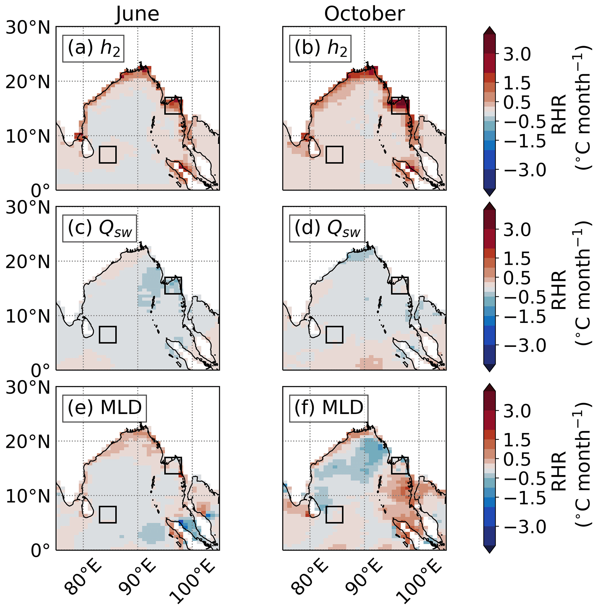
Figure 11 Monthly 29-year average difference (perturbation minus control) of the estimated relative contribution to changes in the radiant heating rate (^∘C month⁻¹) from (a, b) h₂, (c, d) the downward shortwave radiation flux, and (e, f) the MLD for June and October. As in Fig. 10, the black boxes show the location of the open-ocean SMC region and the coastal Irrawaddy Delta region.

In June, the area-weighted mean radiant heating rate difference in the SMC region decreases by 0.1^∘C per month in the perturbation run (Fig. 10a). A decrease in the downward shortwave radiation flux of 5 W m⁻² (Fig. 10c) has the largest contribution to the radiant heating rate decrease of 0.1 ^∘C per month (Fig. 11c), whereas a decrease in h₂ of 2 m and an increase in MLD of 0.4 m (Fig. 10e) contribute less than 0.1 ^∘C per month to the radiant heating rate (Fig. 11a, e). In October, the radiant heating rate difference of the SMC region shows an increase of 0.1 ^∘C per month (Fig. 10b). A decrease in h₂ of 3 m has the largest contribution to the radiant heating rate increase of 0.1 ^∘C per month (Fig. 11b), whereas a decrease in the downward shortwave radiation flux of 1 W m⁻² (Fig. 10d) and an increase in MLD of 0.2 m (Fig. 10f) contribute less than 0.1 ^∘C per month to the radiant heating rate (Fig. 11d, f). In the SMC region, changes in h₂ are smaller than those in coastal regions during June and October. Thus, changes in h₂ and indirect changes in MLD and downward shortwave radiation exert a comparable control on the open-ocean mixed layer radiant heating rate and SST.

The radiant heating rate of the mixed layer and the resultant change in the SST further depend on the seasonal changes in the depth of the mixed layer relative to the solar penetration depth (Turner et al., 2012). Here, we examine how the depth of the mixed layer relative to the solar penetration depth affects mixed layer radiant heating rates and SSTs for the open-ocean region of the SMC and the coastal region of the Irrawaddy Delta during June and October.

Figure 12 Panels (a) to (d) show vertical profiles of the downward shortwave radiation flux from 0 to 60 m for the control (black) and perturbation (green) run for the Irrawaddy Delta region and the SMC region during (a, c)  June and (b, d) October. Panels (e) to (h) show vertical profiles of the radiant heating rate difference from 0 to 60 m during (e, g) June and (f, h) October. Dashed lines show the area-weighted 29-year average mixed layer depth, and coloured dots show the area-weighted average scale depth.

In the Irrawaddy Delta region during October, the MLD shoals to 9 m (green dashed line in Fig. 12b), which is similar to the perturbed h₂ (green dot in Fig. 12b). When the mixed layer is shallow, the increased near-surface radiant heating from reducing h₂ is distributed to a shallower depth, increasing the average change in the radiant heating rate by 1.2^∘C per month (ΔdT ∕dt; Fig. 12f). Below a depth of 10 m, radiant heating rates decrease due to reduced h₂. There is also no change in the MLD in response to reduced h₂ in the perturbation run. The increase of 0.8 m s⁻¹ in the local wind speed is likely to have de-stratifying effects on the upper ocean that oppose the stratifying effects of increased mixed layer radiant heating. When the MLD deepens below 10 m, the biologically induced effects of the increased radiant heating rates above 10 m and the decreased radiant heating rates below 10 m are mixed, reducing the net effect of biological heating on the mixed layer temperature. In June, the MLD deepens to 16 m (Fig. 12a), resulting in a smaller average radiant heating rate change of 0.4 ^∘C per month (Fig. 12e). Consequently, the October SST increases by 0.5 ^∘C compared with the smaller increase of 0.2 ^∘C in June. Hence, shoaling the mixed layer to a depth comparable to the perturbed solar penetration depth in October limits the turbulent mixing processes to a depth where chlorophyll perturbs solar radiation absorption and makes the SST more sensitive to chlorophyll concentration changes.

In the SMC region during October, the MLD shoals to 28 m (Fig. 12d), approximately twice the depth of the perturbed h₂, resulting in an average change in the mixed layer radiant heating rate of 0.1 ^∘C per month (Fig. 12h). As in the Irrawaddy Delta region, there is no change in the MLD in response to biological warming in the SMC region due to the 0.8 m s⁻¹ increase in the local wind speed, which is likely to oppose the stratifying effects of increased mixed layer radiant heating. During June, the MLD extends to 36 m (Fig. 12c), resulting in an average change in the mixed layer radiant heating rate of less than 0.1 ^∘C per month (Fig. 12g). As in the Irrawaddy Delta region, the effect of chlorophyll on upper-ocean temperature depends on the MLD in the SMC region, with the shallowest MLD and largest change in radiant heating rate in October. With lower chlorophyll concentrations in the SMC region than the Irrawaddy Delta region, the resultant change in SMC regional average radiant heating rate in the top 10 m is considerably lower.

4 Discussion and conclusions

In this study, we have identified that the influence of biological warming on the South Asian monsoon strongly depends upon the seasonality of the chlorophyll concentration and the depth of the mixed layer, which is further dependent on the timing of the monsoon itself. The effect of chlorophyll on the SST is amplified during the inter-monsoon periods when shallow MLDs are comparable to the perturbed solar penetration depths. The MLD and its effect on the biological warming vary seasonally and spatially in the BoB. Coastal regions experience larger SST increases than open-ocean regions due to higher chlorophyll concentrations and shallower MLDs. The SST increase is larger during the autumn inter-monsoon (September–October) than during the spring inter-monsoon (April–May) and southwest monsoon onset (June). During the spring inter-monsoon, chlorophyll concentrations are low across the open ocean, but they remain high in coastal regions. During the southwest monsoon onset, chlorophyll concentrations are high when the MLD is relatively shallow (< 30 m) in the northern and western coastal BoB, leading to an increased SST. During the autumn inter-monsoon, high chlorophyll concentrations extend over the continental shelf in the northern BoB, the SMC region, and the eastern BoB, which is in contrast to the spring inter-monsoon when high chlorophyll concentrations are confined to the coasts. The chlorophyll concentrations in the southwestern and northwestern BoB peak in August and October respectively (Lévy et al., 2007), whilst the MLD is shallowest across the basin, which results in an increase in the mixed layer radiant heating rate and SST in the western BoB in autumn.

The direct changes in h₂ in coastal regions are large and, thus, more influential on the mixed layer radiant heating rate and SST. The resultant increase in the radiant heating rate of the coastal mixed layer and SST during the southwest monsoon onset and autumn inter-monsoon increases the latent heat flux and the transport of moisture to the Indian subcontinent. Precipitation rates over the Myanmar coast during the southwest monsoon onset increase by 3 mm d⁻¹. Comparing the monthly average precipitation rate difference (Fig. 4o) with the control simulation bias (Fig. 13a) shows that the model dry bias of 4 mm d⁻¹ over the Myanmar coast is partly removed in the perturbation run. Precipitation rates over western Bangladesh and northeastern India during the autumn inter-monsoon increase by 3 mm d⁻¹. Comparing the precipitation differences (Fig. 7t) with the model bias (Fig. 13b) shows that the model dry bias of up to 3 mm d⁻¹ over northeastern India is removed in the perturbation run. The reduced model biases after imposing a more accurate representation of chlorophyll further highlights the importance of including chlorophyll in coupled models.

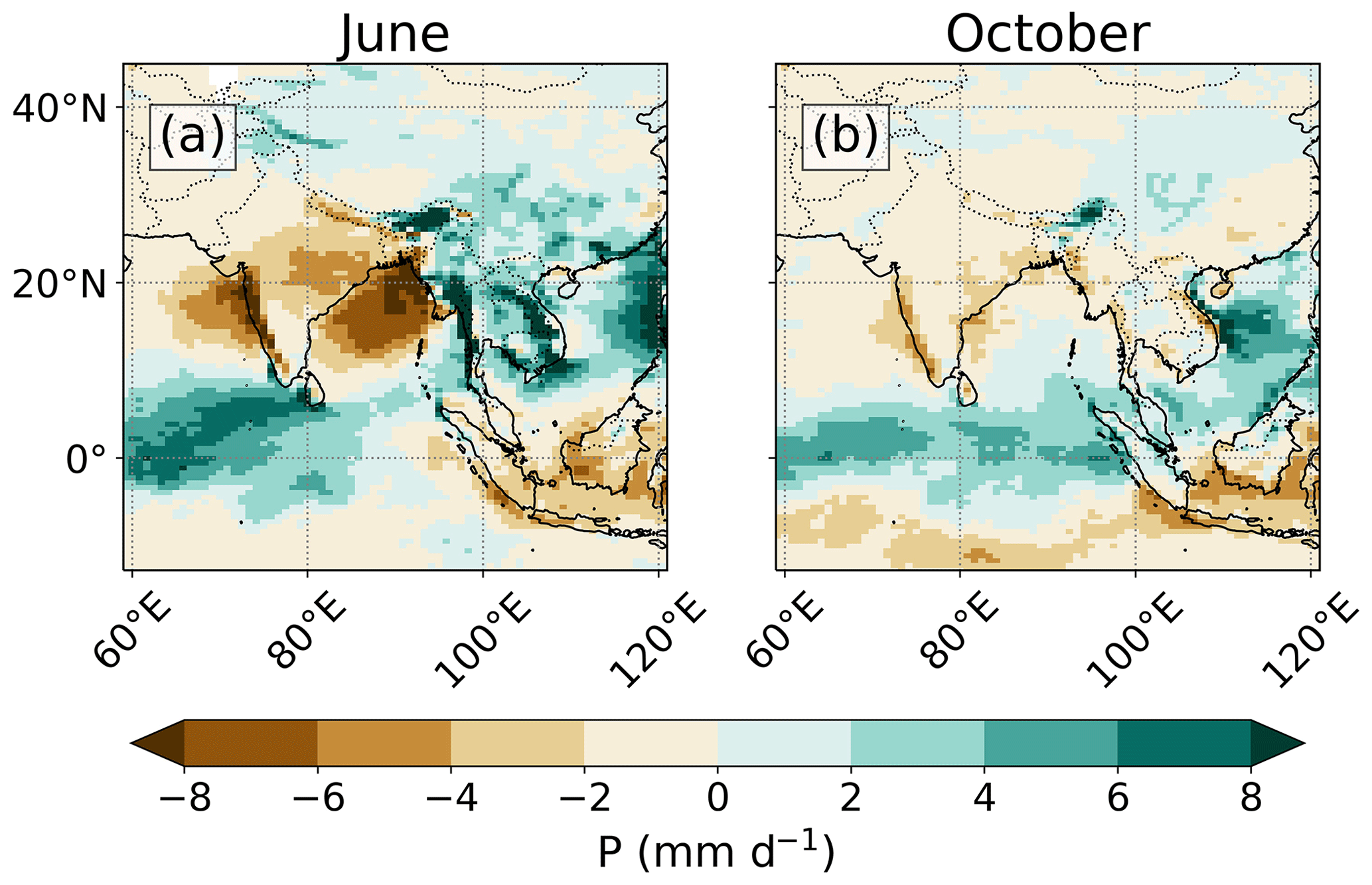
Figure 13 Model bias of the precipitation rate for (a) June and (b) October. Bias calculated as the monthly 29-year average precipitation rate from the control run minus the monthly climatological precipitation rate observed from the TRMM satellite.

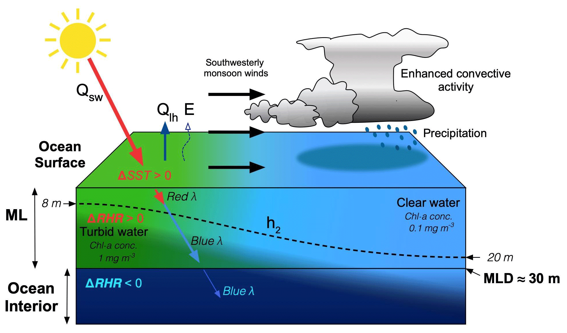
Figure 14 Schematic of the effect of chlorophyll-induced heating on monsoon rainfall in the interior of the BoB. The high chlorophyll concentration in the mixed layer (ML) affects the penetration of the shortwave radiative heat flux (Q_sw), the scale depth of blue light (h₂), and the difference in mixed layer radiant heating rate (ΔRHR) and SST (ΔSST) relative to clear water, which further affects the surface latent heat flux (Q_lh) and evaporation (E). The thick red and blue arrows pointing downwards in the mixed layer illustrate the preferential absorption of the shallow penetrating red light and the deep penetrating blue light respectively. The thin blue arrow pointing downwards below the mixed layer shows the small fraction of penetrative blue light below the mixed layer. The dashed black line in the mixed layer represents h₂. The three solid black arrows across the ocean surface represent the southwesterly monsoon winds transporting heat and moisture that sustain enhanced convection and precipitation over the interior of the BoB.

Figure 14 illustrates and summarizes the effect of chlorophyll during the summer monsoon onset in the BoB interior where mixed layers are shallow (30 m) and where there is a zonal gradient in the mixed layer turbidity. Chlorophyll concentrations are high (1 mg m⁻³) and values of h₂ are low (8 m) to the west, and chlorophyll concentrations are low (0.1 mg m⁻³) and values of h₂ are high (20 m) to the east. The mixed layer radiant heating rates would increase (ΔRHR > 0) in the high chlorophyll concentration region, which reduces the radiant heating rates (ΔRHR < 0) below the mixed layer. Increasing the mixed layer radiant heating rate increases the mixed layer temperature and SST (ΔSST > 0). The upward latent heat flux and evaporation increases with increasing SST and strengthening monsoon winds. Convergence of the additional lower-tropospheric moisture that is transported by the monsoon winds increases the precipitation rates to the east.

During October, the enhanced precipitation rate and convective activity in the northern BoB perturbs upper-tropospheric winds, potentially causing reduced precipitation rates over eastern China, similar to the Silk Road effect. The Silk Road pattern has been found to influence extreme heat waves over eastern China, causing considerable socio-economic devastation (Thompson et al., 2019). Indeed, the model displays significantly warmer surface temperatures in this region at this time (Fig. 9c). The Silk Road pattern dynamics have been previously linked to the South Asian summer monsoon (Stephan et al., 2019). Diverging upper-tropospheric winds caused by precipitation anomalies over the Indian subcontinent interact with midlatitude westerlies, which influences the strength and positioning of the subtropical northwestern Pacific anticyclone over eastern China (Ding and Wang, 2005; Hu et al., 2012a). The effect of chlorophyll on the midlatitude Rossby wave train and its potential impact on the East Asian climate needs further investigation.

Turner et al. (2012) identified a similar modulation of the seasonal SST cycle by the MLD after imposing seasonally varying chlorophyll concentrations in the Arabian Sea. During the spring inter-monsoon, a peak in surface chlorophyll concentrations and shallow MLDs led to an increase in the SST. During the autumn inter-monsoon, another peak in the surface chlorophyll concentration led to a similar but weaker increase in the SST due to deeper MLDs and stronger turbulent surface fluxes. The BoB has less biological productivity than the Arabian Sea due to light and nutrient limitation (Kumar et al., 2002), although chlorophyll concentrations in the coastal BoB can be as high as in the Arabian Sea. The BoB is also exposed to the same monsoonal winds as the Arabian Sea. Such localized, physical forcing modulates the MLD, which, in turn, modulates the biological warming. Hence, the SST increase of 0.5 ^∘C in coastal regions of the BoB during the spring and autumn inter-monsoons is similar to the increase in the SST in the Arabian Sea during the spring inter-monsoon.

Previous studies show that the effect of biological warming is amplified due to secondary feedbacks on the MLD. In the Arabian Sea, high chlorophyll concentrations increase solar radiation absorption and, in turn, thermal stratification, which inhibits vertical mixing, shoals the MLD, and further increases the SST (Nakamoto et al., 2000; Wetzel et al., 2006; Turner et al., 2012). In our study, secondary feedbacks on the MLD are consistent in magnitude with the Arabian Sea studies. The maximum MLD difference is 3 m in the central BoB in June. Coastal MLDs shoaled around the southernmost tip of India and the northern BoB in June by ∼1 m, and the MLDs shoaled around the Kra Isthmus in October by ∼1 m (Fig. 10e, f). The effect of high chlorophyll concentrations in these localized coastal regions appears to have altered upper-ocean thermal stratification when there was little or no change in wind speed, whereas changes in wind speed primarily alter upper-ocean thermal stratification over the majority of the BoB.

In our study, a realistic chlorophyll distribution increased the open-ocean SST by ∼0.1 ^∘C and increased the coastal SST by ∼0.5 ^∘C during the inter-monsoons and southwest monsoon onset. The simulated increase in the open-ocean SST is consistent with previous work (Murtugudde et al., 2002; Wetzel et al., 2006). However, the increase in the coastal SST, primarily in the eastern BoB coastal region, is larger in magnitude than that reported in previous work: Wetzel et al. (2006) underestimated seasonal chlorophyll concentrations in the BoB coastal regions, while Murtugudde et al. (2002) used a low-resolution annual mean chlorophyll concentration which removed the seasonal variability of chlorophyll concentration. In this study, we impose an annual cycle of daily h₂ across the BoB; hence, the coastal and open-ocean SST responses are more accurately represented here than in previous work.

The derivation of the imposed annual cycle of h₂ in coastal regions has limitations. Firstly, the ocean colour algorithms used to determine chlorophyll concentrations from satellite are not completely effective in turbid coastal waters (Morel et al., 2007; Tilstone et al., 2013). Organic and inorganic constituents such as coloured dissolved organic matter (CDOM) and suspended sediments strongly attenuate blue light and are, thus, falsely identified as a chlorophyll-a pigment, which typically leads to an overestimation in chlorophyll concentration (Morel et al., 2007). Secondly, the Morel and Antione (1994) chlorophyll parameterization is not applicable for coastal waters, as the parameterization is based on absorption by chlorophyll-a pigments and not by the attenuation of other in-water constituents. Missing h₂ values in the Ganges River delta are interpolated from neighbouring h₂values that are likely associated with a satellite product and parameterization uncertainty. The Ganges coastal region has been found to influence the spring inter-monsoon SST and precipitation rates in the northern BoB. Possible positive biases in the chlorophyll concentration in the Ganges River delta are likely to lead to an overestimation of the coastal biological warming, SST, and precipitation rate increase. Ocean colour algorithms to determine proxy coastal chlorophyll concentrations are still an area of active research (Blondeau-Patissier et al., 2014). Future studies should consider the attenuation of solar radiation from other oceanic constituents in turbid coastal regions to better represent radiant heating in the upper ocean.

CDOM is a common oceanic constituent that perturbs solar penetration depths. The derived values of h₂ incorporate the bio-optical property of the chlorophyll-a pigment concentration, largely excluding CDOM. CDOM increases the radiant heating rate of nearshore coastal waters of North America (Chang and Dickey, 2004) and the Arctic (Hill, 2008). Imposing an annual mean of remotely sensed CDOM absorption coefficients in a coupled ocean–atmosphere GCM reduced solar penetration depths and increased the coastal SST in the Northern Hemisphere during the summer (Kim et al., 2018). CDOM concentrations are high in the western and northern coastal regions of the BoB at the mouths of major rivers (Pandi et al., 2014). Thus, including the bio-optical properties of CDOM and other biological constituents would likely increase the coastal SST in the BoB, with additional implications for regional climate.

The chlorophyll concentration in the BoB upper ocean is not homogeneous with depth. In situ observations show that the vertical depth of chlorophyll maxima varies between 10 and 80 m (Thushara et al., 2019; Pramanik et al., 2020), often occurring at depths undetected by satellite radiometer sensors (Huisman et al., 2006). Variations in the vertical depth of the chlorophyll maxima would vary the vertical depth of enhanced radiant heating. However, if the depth of the chlorophyll maxima occurs at a depth where solar radiation is significantly reduced (e.g. at the euphotic depth where solar radiation is ∼1 % of its surface value), the change in the local radiant heating at that depth would be negligible (Morel and Antione, 1994). Indeed, observations show the occurrence of intense deep chlorophyll maxima in the BoB at depths from 20 to 40 m (Thushara et al., 2019), which might have a strong influence on local mixed layer radiant heating and vertical heat distributions. Hence, the effect of nonuniform chlorophyll concentration profiles on upper-ocean radiant heating and SST requires further investigation.

The mesoscale and sub-mesoscale spatial variability of h₂ and the associated oceanic processes is inadequately represented in MC-KPP due to its coarse horizontal resolution. The coastal region in MC-KPP is represented by multiple grid points that are part ocean and part land at an approximate 90 km horizontal resolution. Such a resolution means that at the coastlines, the mesoscale coastal chlorophyll concentration features, and the corresponding solar penetration depths are poorly resolved. Future studies should consider using a high-resolution, fully dynamical model to accurately resolve the coastline and the associated solar penetration depths. The simulated dynamics would improve the representation of mesoscale eddy activity along the coast and open ocean, which increases biological productivity (Kumar et al., 2007) and, in turn, increases local solar radiation absorption.

The sub-seasonal temporal variability of h₂ is inadequately represented in MC-KPP due to the use of a monthly mean climatological chlorophyll concentration at a reduced horizontal resolution. In reality, the advection of high surface chlorophyll concentrations into the southern and central BoB varies with the strength and positioning of the SLD and SMC (Vinayachandran et al., 2004), which is itself further influenced by local wind stress and seasonal Rossby waves (Webber et al., 2018). Surface chlorophyll concentrations are periodically enhanced by transient cold-core eddies and post-monsoon cyclones in the central BoB, which briefly upwell nutrients to the ocean surface (Vinayachandran and Mathew, 2003; Patra et al., 2007). In coastal regions, nutrient concentrations, which affect surface chlorophyll concentrations, vary with river discharge (Kumar et al., 2010). Suspended terrestrial sediment that perturbs solar penetration depths on the continental shelf also depend on river discharge (Kumar et al., 2010; Lotliker et al., 2016). All of these factors influence solar penetration depths on timescales of days to weeks and on spatial scales of less than 1 km. By smoothing over the large sub-seasonal variability of the chlorophyll concentration, such variations in the solar penetration depth are not represented in the present study.

The limitations of representing ocean dynamics as a mean seasonal cycle means that MC-KPP cannot capture any ocean dynamical response to biologically induced changes in ocean properties (e.g. changes in ocean temperature and salinity transports). Previous studies have shown large effects of chlorophyll on ocean dynamics in the equatorial Pacific (e.g. Nakamoto et al., 2001; Murtugudde et al., 2002) and in mid- to high-latitude regions (e.g. Manizza et al., 2005; Patara et al., 2012). Modified biological warming at the surface or perhaps modified solar radiation penetration below the mixed layer could affect the dynamics of the SMC and SLD in the BoB. Missing modes of variability in MetUM-GOML that rely on a dynamical ocean, such as ENSO and IOD, could combine nonlinearly with the ocean anomalies induced by biological warming, with implications for monsoon rainfall. Further research using a fully dynamical coupled ocean–atmosphere GCM is required to show the dynamical changes and feedbacks of biological warming on the BoB oceanic and atmospheric system.

Biological heating has complex physical and dynamical feedbacks in the ocean, which, in turn, imply similar feedbacks on BoB biological processes. The imposed seasonally and spatially varying h₂ in MC-KPP eliminates any biological response to secondary feedbacks in the ocean. A coupled biogeochemistry model linked to an ocean–atmosphere GCM would be needed to further understand secondary feedbacks on phytoplankton productivity. Secondary feedbacks may include changes in cloud cover that affect the incoming shortwave radiation needed for biological productivity, changes in thermal and salinity stratification that affect the vertical mixing of nutrients to the ocean surface, or changes in rainfall that affect river discharge and nutrient availability on the continental shelf which influence biological productivity. The resultant changes in biological productivity could either enhance or deplete chlorophyll concentrations at the surface, with further implications for the spatial and temporal extent of biological heating. It is important that realistic simulations of chlorophyll concentrations are included as an additional Earth system process in high-resolution coupled ocean–atmosphere GCMs, which may improve the simulated seasonality and intraseasonal variability of the South Asian monsoon.