the Creative Commons Attribution 4.0 License.
the Creative Commons Attribution 4.0 License.
 | 29 Oct 2021
The impact of deep convection representation in a global atmospheric model on the warm conveyor belt and jet stream during NAWDEX IOP6
Meryl Wimmer
Philippe Arbogast
Jean-Marcel Piriou
Julien Delanoë
Carole Labadie
Quitterie Cazenave
Jacques Pelon
The effect of parameterized deep convection on warm conveyor belt (WCB) activity and the jet stream is investigated by performing simulations of an explosively developing large-scale cyclone that occurred during the North Atlantic Waveguide and Downstream Impact Experiment (NAWDEX) field campaign using the Météo-France global atmospheric model ARPEGE. Three simulations differing only from their deep convection representation are analysed. The first one was performed with the Bougeault (1985) scheme (B85), the second one with the Prognostic Condensates Microphysics and Transport (PCMT) scheme of Piriou et al. (2007), and the third one without any parameterized deep convection. In the latter simulation, the release of convective instability at the resolved scales of the model generates localized cells marked by strong heating with few degrees extent in longitude and latitude along the fronts. In runs with active parameterized deep convection (B85, PCMT), the heating rate is more homogeneously distributed along fronts as the instability release happens at subgrid scales. This difference leads to more rapid and abrupt ascents in the WCB without parameterized deep convection and more moderate but more sustained ascents with parameterized deep convection. While the number of WCB trajectories does not differ much between the three simulations, the averaged heating rates over the WCB trajectories exhibits distinct behaviour. After 1 d of simulations, the upper-level heating rate is on average larger, with the B85 scheme leading to stronger potential vorticity (PV) destruction. The difference comes from the resolved sensible and latent heating and not the parameterized one. A comparison with (re)analyses and a large variety of airborne observations from the NAWDEX field campaign (Doppler radar, Doppler lidar, dropsondes) made during the coordinated flights of two aircraft in the WCB outflow region shows that B85 performs better in the representation of the double jet structure at 1 d lead time than the other two simulations. That can be attributed to the more active WCB at upper levels. However, this effect is too strong and that simulation becomes less realistic than the other ones at forecast ranges beyond 1.5 d. The simulation with the PCMT scheme has an intermediate behaviour between the one with the B85 scheme and without parameterized deep convection, but its impact on the jet stream is closer to the latter one. Finally, additional numerical experiments show that main differences in the impact on the jet between PCMT and B85 largely come from the chosen closure, with the former being based on CAPE and the latter on moisture convergence.
- Article
(13148 KB) - Full-text XML
-
Supplement
(753 KB) - BibTeX
- EndNote


Despite significant and continuous improvements of numerical weather forecasts during the last decades (Simmons and Hollingsworth, 2002; Bauer et al., 2015), mid-latitude weather forecast errors still occur at synoptic and planetary scales. For instance, at short-range (days 1–3) weather forecasts still struggle to accurately predict the intensity, timing, and location of extratropical storms (Korfe and Colle, 2018) and in particular their wind gusts footprints (Hewson et al., 2014). At medium range (days 4–8), forecast busts may occur in the prediction of large-scale atmospheric circulation patterns like blockings (Rodwell et al., 2013; Grams et al., 2018; Maddison et al., 2020). Forecast errors are usually characterized by an upscale and downstream error growth (Zhang et al., 2007; Selz and Craig, 2015), which start at the convective scale and mesoscale (Rodwell et al., 2013). They then often propagate downstream and amplify along upper-tropospheric Rossby wave trains (Gray et al., 2014; Lillo and Parsons, 2017) where nonlinear effects are strong (Baumgart et al., 2018). They finally form large-scale forecast error patterns further downstream, typically at the end of storm tracks like over western Europe (Grams et al., 2018; Maddison et al., 2020).
These forecast errors originate from two main sources of uncertainties: uncertainties in determining the initial state of the atmosphere and uncertainties due to the imperfections of numerical weather prediction (NWP) models (Tribbia and Baumhefner, 1988). But it is somewhat difficult to determine the origins of forecast busts among these two sources as they intertwine and can compensate for or reinforce each other (Rodwell et al., 2013). Among the model deficiencies, the representation of subgrid-scale physical processes (e.g. cloud microphysics, convection, radiation, turbulence) by different parametrization schemes is a key question and such schemes are constantly upgraded.
The question of the impact of diabatic processes on the predictability of the atmospheric flow was central to the international NAWDEX (North Atlantic Waveguide Downstream and impact Experiment) project and its field campaign that occurred in September–October 2016 (Schäfler et al., 2018). In particular, one main hypothesis of the project is that the potentially misrepresented diabatic processes embedded in the so-called warm conveyor belts (WCBs) play a key role in triggering forecast errors along the North Atlantic upper-tropospheric waveguide. They may significantly deteriorate the forecast of high-impact weather events more downstream. WCBs correspond to air masses flowing within the boundary layer in the warm sector of extratropical cyclones and ascending to the tropopause level east of the cyclone centre (Browning, 1990; Wernli and Davies, 1997). These coherent air masses make the connections between the different layers of the troposphere as they gain moisture in the boundary layer, undergo heat release by condensation when they ascend and have an impact on the upper-tropospheric circulation. When they reach the tropopause level, negative potential vorticity (PV) is generated in the WCB outflow region that reinforces the ridge downstream of the cyclone but also the upper-tropospheric PV gradient and hence the jet stream (Pomroy and Thorpe, 2000; Grams et al., 2011; Schemm et al., 2013; Chagnon et al., 2013; Gray et al., 2014). Uncertainties in the heat release within WCBs due to misrepresented cloud microphysics or convection could trigger forecast errors at the tropopause level that may then propagate downstream along the waveguide (Martinez-Alvarado et al., 2016; Grams et al., 2018; Maddison et al., 2020). The objective of the present study is to investigate the effect of parameterized deep convection in a global NWP model on the WCB activity and the jet stream.
Embedded convective activity within WCBs was initially identified using airborne and satellite-derived data within an extratropical cyclone during the Experiment on Rapidly Intensifying Cyclones over the Atlantic (ERICA) field experiment (Neiman et al., 1993). Various ground-based, spaceborne and airborne remote sensing measurements confirm the regular presence of convective activity in the warm sector of extratropical cyclones and WCBs in particular (Crespo and Posselt, 2016; Flaounas et al., 2016, 2018; Oertel et al., 2019; Blanchard et al., 2020; Jeyaratnam et al., 2020). This was detected in various regions of the Northern Hemisphere: over the United States (Jeyaratnam et al., 2020), the North Atlantic ocean (Crespo and Posselt, 2016; Oertel et al., 2019, 2020, 2021; Blanchard et al., 2020, 2021) and in the Mediterranean sector (Flaounas et al., 2016, 2018). Recent numerical studies relying on convection-permitting model simulations of various extratropical cyclones also highlighted the presence of embedded convection within WCBs (Rasp et al., 2016; Oertel et al., 2019, 2020, 2021; Blanchard et al., 2020, 2021). The emerging picture is that WCBs are composed of various ascending air streams in which convective ascents may intermittently happen within the main slantwise ascending airflow. Such an intermittent convective activity may have non-negligible effects on the upper-level jet stream. Oertel et al. (2020) and Blanchard et al. (2021) showed that the WCB-embedded convective cells form dipolar PV anomalies with the negative pole being closer to the jet which tend to reinforce the PV gradient and hence the jet.
Because WCB-embedded convection plays an important role in the large-scale circulation, it is worth investigating the effect of parameterized deep convection on WCBs in models that do not have enough resolution to explicitly resolve that phenomenon. The contribution of parameterized convection in the total heating and precipitation rates within extratropical cyclones varies a lot by changing schemes as shown by Martinez-Alvarado et al. (2014b) and Booth et al. (2018). Differences in total precipitation rates between models usually vary much less than differences in the contribution of parameterized convection to the total. Done et al. (2006) showed that the upper-level large-scale circulation is sensitive to the relative amount of parameterized vs. explicit convection, but their focus was on the effect of mesoscale convective systems and not WCBs of deep cyclones. More relevant to the present study, the impact of convection parametrization on WCB dynamics and its effect on the upper-level flow was studied by Martinez-Alvarado and Plant (2014) in a case study of a North Atlantic extratropical cyclone. The authors show that parameterized convection “regulates the action of large-scale heating” by releasing convective instability at subgrid scales which would have otherwise been released at larger and resolved scales. Because of this regulation, WCB trajectories more gradually ascend when parameterized convection is more active than when it is reduced. Furthermore, in the presence of reduced parameterized convection, the more abrupt ascents lead to more important impact on upper-level circulation even though differences with active parameterized convection are small at 24 h lead time (Martinez-Alvarado et al., 2014a). In the same vein, the present study aims to address the following questions.
-
How different are WCBs between simulations with active parameterized deep convection and those without?
-
What is the impact of parameterized deep convection on the jet stream at short range (less than 2 d)?
-
How different are WCBs and their impact on the jet stream between simulations performed with distinct deep convection schemes?
Our approach is based on the case study of an extratropical cyclone that occurred during NAWDEX called the Stalactite cyclone (29 September–3 October 2016) and corresponding to Intensive Observing Period (IOP) 6. It was an explosively deepening cyclone at a rate of roughly 24 hPa in 24 h (Flack et al., 2021) that formed off the east coast of Newfoundland and travelled over the North Atlantic toward Iceland and Greenland. This large-scale cyclone participated in the formation of a block over Scandinavia (Schäfler et al., 2018). The Stalactite cyclone was already the subject of several studies. Maddison et al. (2019, 2020) showed that the low predictability of the block onset at medium range was associated with uncertainties in the timing, location and intensity of that cyclone. Blanchard et al. (2020) and Blanchard et al. (2021) studied the WCB-embedded convection by performing convection-permitting model simulations, while Mazoyer et al. (2021) analysed the impact of cloud microphysics on the WCB activity of the Stalactite cyclone with similar convection-permitting simulations. Flack et al. (2021) analysed the whole life cycle of the cyclone in simulations of two climate models. Maddison et al. (2020) showed that medium-range forecast skills of the cyclone are sensitive to the choice of the deep convection schemes, but none of these studies systematically investigated the role of parameterized deep convection on the WCB of the cyclone at short range. In addition to its dynamical interest, the Stalactite cyclone is worth studying because numerical simulations can be compared and validated against airborne observations: two flights of the French Falcon 20 from the Service des Avions Français Instrumentés pour la Recherche en Environnement (SAFIRE) and one flight from the Deutsches Zentrum für Luft- und Raumfahrt (DLR) Dassault Falcon were conducted on 2 October 2016.
The paper is structured as follows. Section 2 is dedicated to the method where the global atmospheric model ARPEGE (Action de Recherche Petite Echelle Grande Echelle) and the three numerical simulations are presented. Two simulations are run with two distinct deep convection schemes used and developed within ARPEGE. The first one is used in the deterministic operational forecasts of the NWP version of the model and was developed by Bougeault (1985), while the second, called the Prognostic Condensates Microphysics and Transport scheme and developed by Piriou et al. (2007), was implemented in the CMIP6 version of the ARPEGE climate model (Roehrig et al., 2020). A third simulation is performed in which the deep convection scheme is turned off. The Lagrangian trajectory algorithm, PV diagnostics, and the reanalysis and airborne observation datasets are also summarized in Sect. 2. In Sect. 3, the impact of deep convection schemes on heating rates and WCB trajectories is analysed, while Sect. 4 is focused on their effect on the upper-level circulation and the jet stream. Finally, Sect. 5 provides concluding remarks.
2.1 Model and simulations set-up
The Météo-France global forecast model ARPEGE (Courtier et al., 1991) is used at a T798 resolution with full physics and 90 vertical levels. The stretched horizontal grid (mapping factor of 2.4) corresponds to about 10 km horizontal resolution over France, 15 km near Iceland and 60 km on the opposite side of the globe relative to France. The temporal resolution is 7.5 min. Simulations analysed in the present study are based on the 2016 operational version of the ensemble prediction system (EPS) of ARPEGE called the Prévision d'Ensemble ARPEGE (PEARP; Descamps et al., 2015). It is documented in Ponzano et al. (2020) (see their Table 1) and was already used to study the predictability of a heavy precipitation event that occurred over France during NAWDEX (Binder et al., 2021). It includes 10 members that have the same initial state, which is the ARPEGE operational analysis made with a 4D-Var data assimilation scheme. They only differ in the representation of at least one of the following physical packages: deep convection, turbulence, shallow convection and surface oceanic fluxes. Two largely distinct deep convection schemes are used: one is the scheme developed by Bougeault (1985), hereafter called B85, and the other one is the Prognostic Condensates Microphysics and Transport scheme of Piriou et al. (2007), hereafter called PCMT. For some members, modified versions of B85 are activated. Two turbulent schemes are used: the turbulent kinetic energy scheme of Cuxart et al. (2000) and the turbulence scheme of Louis (1979). Four shallow convection schemes are considered: the mass flux scheme of Kain and Fritsch (1993) and Bechtold et al. (2001), PCMT, the eddy diffusivity and Kain–Fritsch scheme, and the Pergaud et al. (2009) scheme. Surface oceanic fluxes are represented by the Belamari (2005) scheme or by an alternate version in which the evaporative fluxes are enhanced. The paper is focused on two particular members of this EPS, corresponding to the REF member and seventh member respectively as it appears in Table 1 of Ponzano et al. (2020). They only differ in the representation of deep convection, one using the B85 scheme and the other the PCMT scheme. The two simulations share the same physical parameterizations for turbulence (turbulent kinetic energy scheme; Cuxart et al., 2000), shallow convection (Kain and Fritsch, 1993; Bechtold et al., 2001), large-scale microphysics (Lopez, 2002) and oceanic flux (Exchange Coefficients from Unified Multi-campaigns Estimates; Belamari, 2005). Finally, a third simulation is performed without any active deep convection scheme (hereafter called NoConv) but with the same other physical packages as the other two simulations and will serve as a reference to assess the impact of B85 and PCMT schemes.
The three simulations are hereafter systematically compared. The starting time and date are 12:00 UTC on 1 October 2016 when the surface cyclone is already in its mature stage and located in the middle of the North Atlantic (see the position of the minimum sea level pressure at 1 d lead time in Fig. 1).
2.1.1 The Bougeault (1985) deep convection scheme
This mass flux scheme is triggered when the resolved plus subgrid-scale moisture convergence is positive in the low levels and the atmospheric profile is unstable. So the scheme is closed with moisture convergence. Following Kuo (1965) the total moisture convergence is either detrained in the convective environment or precipitated. This scheme was further developed by Ducrocq and Bougeault (1995) for downdraughts. It is part of the global operational NWP (numerical weather prediction) system at Météo-France and is currently used to perform ARPEGE deterministic operational simulations.
2.1.2 The Prognostic Condensates Microphysics and Transport scheme of Piriou et al.(2007)
This convection scheme separates microphysics and transport in grid-scale equations to overcome stationary cloud budget assumptions, as proposed by Piriou et al. (2007). Liquid and ice cloud condensates, as well as rain and snow, have prognostic mixing ratios to deal with the same level of sophistication inside convective updraught as in the resolved-scale microphysics (Lopez, 2002; Bouteloup et al., 2011), therefore including autoconversion, aggregation, collection, riming, melting, etc. The closure of all experiments run with PCMT in the present study is based on CAPE (convective available potential energy). As previously said, this scheme is used in PEARP but also is part of the CNRM Earth System Model for CMIP6 (Roehrig et al., 2020).
2.2 Model output and diagnostics
The output datasets of the simulations are provided on a regular longitude–latitude grid of 0.5∘, a pressure grid spacing of 50 hPa in the vertical and a frequency of 15 min.
2.2.1 WCB trajectories
The Lagrangian trajectory code is designed to work with latitude × longitude × pressure files of zonal wind u, meridional wind v, vertical velocity ω, and other variables such as temperature and diabatic tendencies. The algorithm is based on a prediction-correction method of the advection at the midpoint of the trajectory. Let DT be the time interval between two model outputs. To account for curvature effects, the trajectory model has higher resolution than the model outputs, and its time step dt is such that DT. At dt (where ) and for each point (p denotes pressure, x and y are horizontal coordinates) belonging to a trajectory, we look for the previous position , with the advection being made with u, v and ω in the middle of the trajectory portion at , which is not known a priori. We first apply a time interpolation to compute the 3D wind field at time t using the two closest model outputs for at time i× DT and and referred to as . We then apply an iterative method starting with the wind at the point of the trajectory at time t (i.e. ) to build up a first estimation of the previous position of the trajectory and extract the wind along this first estimated trajectory at (called ) by horizontal, vertical and time interpolation. Horizontal interpolation is bilinear (four neighbouring points are used). A second estimated trajectory is calculated using U1, leading to a second estimation of the previous position . The process can be repeated several times, but practical tests show it converges after about two iterations. If a trajectory goes beyond 975 hPa, its position is shifted to 975 hPa. Note that such an algorithm allows the computation of both backward and forward trajectories. In what follows, DT and dt are equal to 15 and 7.5 min respectively (n=2).
Forward trajectories are initialized at 12:00 UTC on 1 October in the warm sector of the extratropical cyclone and computed during 48 h. To select WCB trajectories, a criterion of ascent exceeding 300 hPa within 1 d during the period between 12:00 UTC on 1 October and 12:00 UTC on 3 October is applied. This is a less strict criterion than the more usual criterion of 600 hPa ascent within 2 d (Madonna et al., 2014; Binder et al., 2016) but allows a broad view of the different ascents in the WCB.
2.2.2 Heating and PV tendencies
The Ertel potential vorticity q and its Lagrangian derivative can be expressed as (Ertel, 1942)
where is the Lagrangian derivative, θ is the potential temperature, ρ is density, ζa is the three-dimensional absolute vorticity vector, ∇ is the three-dimensional gradient and F is the three-dimensional frictional acceleration. The diabatic heating is denoted as . These two equations can be rewritten under the hydrostatic balance in pressure coordinates as
where Fx and Fy are the zonal and meridional components of the frictional acceleration. Even though the friction-induced PV tendency is not negligible and generally generates a positive PV anomaly in lower troposphere (Stoelinga, 1996), it is not shown in the present study which is focused on the upper-level PV modification. PV modification along WCB has been generally attributed to the term involving the vertical gradient of the diabatic heating (Wernli and Davies, 1997; Joos and Wernli, 2012) – that is, the first term on the right-hand side of Eq. (4). The second and third terms involving the horizontal gradient of the heating have been generally considered to be second-order effects. Very recently the horizontal gradient has been shown to be very important in high-resolution convection-resolving simulations (Oertel et al., 2020).
The first method to compute the diabatic heating consists of approximating the time and space derivatives of potential temperature using centred finite-difference schemes applied to the potential temperature over the 0.5∘ × 0.5∘ horizontal grid and 50 hPa vertical grid and with a frequency of 15 min. An alternative to compute the total heating is to sum all the temperature tendencies due to each physical process (resolved and parameterized sensible and latent heating, radiation, turbulence) that are made available as model outputs on a non-regular grid. Spatial interpolations were necessary to get them on the same regular 0.5∘ × 0.5∘ grid of the model outputs. The total heating obtained with this second method was found to be less accurate to represent the change in potential temperature undergone by the Lagrangian trajectories. Hence the first method based on centred finite-difference schemes is used to make all the main figures of the paper. The second method is only used in some Supplement to show the robustness of the results as well as to attribute the total heating to some specific physical processes, which cannot be provided by the first method. It is not surprising that the first method accurately approximates the potential temperature variations along trajectories because the computations of both the trajectories and the finite differences are made on the same grid and, in that sense, are self consistent. The second method less well approximates the potential temperature variations along trajectories because the post-process treatment to get the individual diabatic temperature tendencies and the underlying interpolations were not the same as for the other variables (wind, temperature). Finally, to get the PV tendencies due to the heating (first three terms on the right-hand side of Eq. 4), centred finite-difference schemes are applied to the heating.
2.3 Reanalysis and observations
2.3.1 Reanalysis and operational analysis
Operational analyses from ARPEGE and the Integrated Forecasting System (IFS) of the European Centre for Medium-Range Weather Forecasts (ECMWF) are used on the same regular latitude–longitude grid with 0.5∘ resolution and the same pressure levels with 50 hPa spacing as the model simulations outputs. ERA5 reanalysis datasets (Hersbach et al., 2020) are also used with the same 0.5∘ grid spacing – that is, keeping one grid point every two grid points from the 0.25∘ original grid of the reanalysis.
2.3.2 Airborne observations and comparison to model outputs
Two coordinated flights of the SAFIRE and DLR Falcon aircraft were conducted from 09:00 to 12:00 UTC on 2 October between Iceland and Greenland to sample the WCB outflow region of the Stalactite cyclone. The two aircraft followed each other with a 10 min interval between 09:00 and 10:15 UTC. The 95 GHz Doppler cloud radar RASTA (Radar Airborne System Tool for Atmosphere; Delanoe et al., 2013) on board the SAFIRE Falcon measured both reflectivity and Doppler velocity along three antennas (nadir, backward and transverse) that allow for reconstructing the three wind components. The temporal resolution between two consecutive nadir measurements being 750 ms and the typical Falcon 20 speed 200 m s−1, the horizontal resolution is near 300 m. Additional wind measurements were made during the flight of the SAFIRE Falcon by launching nine dropsondes and by in situ sensors at the aircraft level. The 2 µm scanning coherent/heterodyne detection Doppler wind lidar (DWL; Weissmann et al., 2005; Witschas et al., 2017) on board the DLR Falcon measured vertical profiles of line-of-sight wind speed, horizontal wind vectors and detected aerosol/cloud layers.
Since the model output grid is 0.5∘ × 0.5∘, which corresponds to 28 km × 55 km spacing in longitude and latitude respectively, the radar RASTA and DWL wind measurements are averaged over intervals of 180 s to get the same horizontal resolution as the model outputs (the Falcon travels a distance of 36 km in 180 s).
3.1 General overview
Differences in sea level pressure (SLP) between the three integrations are rather small (Fig. 1). The tracks of the minimum SLP are rather similar, and differences in the minimum SLP do not go beyond 2 hPa at 1 d lead time (962.9 hPa in B85, 962.0 hPa in PCMT and 961.2 hPa in NoConv) or at 2 d lead time (959.5 hPa in B85, 959.8 hPa in PCMT and 958 hPa in NoConv). This subsection is more particularly dedicated to presenting differences in the main characteristics of the WCB between the three runs. The number of trajectories satisfying the WCB criterion of the present study (ascent rate of at least 300 hPa in 24 h) does not differ much between the three runs: 9876, 10 086 and 11 421 for B85, PCMT and NoConv simulations respectively. The WCB trajectories share many common features between the runs. A majority of trajectories exhibit a well-marked cyclonic curvature during their ascents to the east of the surface cyclone and then change their curvature in the upper troposphere over Greenland to become more zonally oriented and slightly anticyclonically curved toward Scandinavia (Fig. 1). These trajectories in the upper troposphere span a larger latitudinal band in NoConv than PCMT and B85 (compare the banded areas formed by the blue segments of the trajectories). The largest difference between the three runs concerns another set of trajectories that has a more zonal orientation from the mid-Atlantic to western Europe near 45∘ N. There are very few such trajectories in the B85 run, while they are more abundant in the PCMT run and are very numerous in the NoConv run.
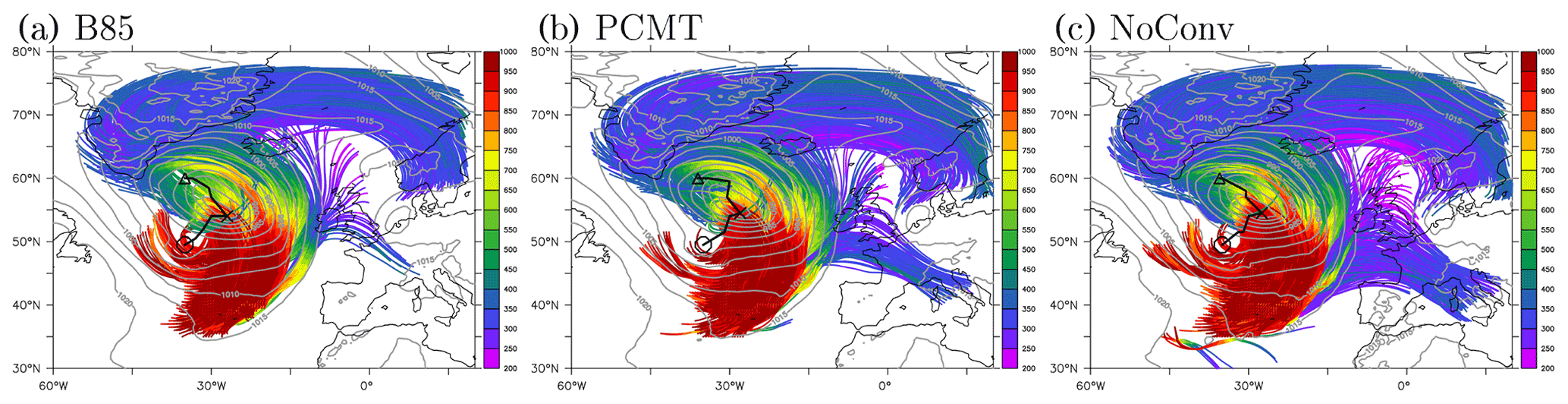
Figure 1WCB trajectories from 12:00 UTC on 1 October to 12:00 UTC on 3 October coloured according to pressure (in hPa) for (a) B85, (b) PCMT and (c) NoConv simulations. The sea level pressure at 12:00 UTC on 2 October is shown in grey contours (interval: 5 hPa). Only WCB trajectories with an ascent criterion of at least 600 hPa in 48 h are shown for clarity purposes. In each panel, the black thick line represents the track of the minimum sea level pressure of the corresponding run between 12:00 UTC on 1 October and 12:00 UTC on 3 October. The circle, cross and triangle correspond to the position of the minimum sea level pressure at 12:00 UTC on 1 October, 12:00 UTC on 2 October and 12:00 UTC on 3 October respectively.
Figure 2 presents averaged quantities along the WCB trajectories of the three runs. The mean pressure is about 894 hPa at 12:00 UTC on 1 October for the three runs and reaches 415 hPa for B85, 427 hPa for PCMT and 435 hPa for NoConv at 12:00 UTC on 3 October. Some differences also appear in the 90th percentile, with the WCB trajectories of the B85 run having systematically lower pressure levels than the other two runs (Fig. 2a). There are not so many differences between the mean potential temperatures of the three runs. The only notable difference is the slightly higher mean temperature in the B85 run than in the other two runs from 12:00 UTC on 2 October to 12:00 UTC on 3 October (Fig. 2b). This difference between B85 and PCMT is significant at the 99 % level following a Welch test, while differences with NoConv are not significant. The time evolution of the PV along WCB trajectories is characterized by an increase followed by a decrease (Fig. 2c), which is a classical picture of WCBs as they undergo PV production at low levels below the heating layer and PV destruction at upper levels above the heating layer (e.g. Wernli and Davies, 1997; Schemm et al., 2013). Differences in PV between the three runs are more important than differences in pressure or potential temperature. Trajectories of B85 and PCMT runs undergo a more important increase and decrease of PV than those of the NoConv run on average. While the two runs with activated parameterized convection exhibit a similar increase in PV during the first 24 h, they differ in the subsequent decrease in PV. B85 trajectories exhibit a more rapid decrease in PV between 18:00 UTC on 2 October and 00:00 UTC on 3 October, while PCMT trajectories show a smoother decrease in PV.
To get a better insight on the heating and PV evolution along trajectories, Fig. 3 shows the time evolution of the mean vertical profile of the heating and PV tendency due to the vertical gradient of the heating along WCB trajectories. While the magnitudes of the heating and PV tendency are rather similar between the three runs, some significant differences also appear. The NoConv case exhibits the strongest heating values at the early stage (18:00 UTC on 1 October) but the lowest ones at the later stage (18:00 UTC on 2 October to 06:00 UTC on 3 October) compared to the other two cases, suggesting a more rapid destabilization of the atmosphere in NoConv. In terms of PV, the expected picture of PV gain and loss below and above the main heating layer respectively is visible for the three cases. We observe that the PV gain region presents two peaks between 12:00 UTC on 1 October and 12:00 UTC on 2 October, one in the boundary layer and another near 700–800 hPa. But more importantly, the negative PV tendency above the heating layer is stronger for B85 than PCMT and NoConv during the whole period and in particular between 18:00 UTC on 2 October and 00:00 UTC on 3 October when WCB trajectories reach these upper levels. Such a difference is also seen by computing the total PV tendency due to the heating, i.e. by summing the first three terms on the right-hand side of Eq. (4) (not shown), and is in agreement with the more rapid decrease in PV seen in Fig. 2c for B85. This difference is mainly due to the fact that the heating reaches higher values in the upper troposphere between 2 and 3 October in B85 and thus has stronger vertical gradients (e.g. see the more important tightening of black contours between 00:00 UTC on 2 October and 00:00 UTC on 3 October in Fig. 3a than Fig. 3b, c).
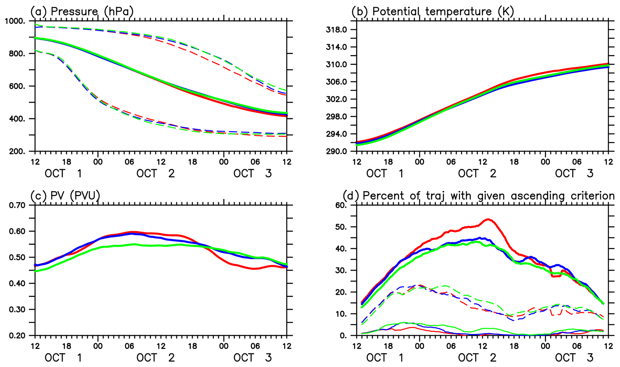
Figure 2Time evolution along WCB trajectories of (a) mean pressure (solid lines, units: hPa) and the 10th and 90th percentiles of pressure (dashed lines), (b) mean potential temperature (solid lines; units: K), and (c) mean PV (units: PVU). Panel (d) indicates the percentage of WCB trajectories in each run satisfying a given ascending criterion at a given time: 100 hPa in 2 h (light solid lines), 50 hPa in 2 h (dashed lines) and 25 hPa in 2 h (bold solid lines). The red, blue and green curves correspond to B85, PCMT and NoConv simulations respectively.
Let us now document differences in the instantaneous ascending motion of the trajectories between the three runs. The proportion of trajectories ascending by more than 100, 50 and 25 hPa in 2 h between T−1 h and T+1 h is indicated as function of time T in Fig. 2d. NoConv has the largest number of trajectories ascending most rapidly (i.e. 100 hPa within 2 h and 50 hPa within 2 h), B85 is the run having the lowest number, and PCMT is in between regardless of the time. In the category of more modest ascents (25 hPa in 2 h), B85 has more such trajectories in proportion than the other two runs from 00:00 to 18:00 UTC on 2 October. Beyond 18:00 UTC on 2 October, the proportions of moderately ascending trajectories are closer to each other between the three runs. These differences in the ascending motion properties are synthesized in Fig. 4. The NoConv trajectories undergo the most rapid vertical motion with a maximum vertical displacement of about 104 hPa in 2 h when averaged over all trajectories. In comparison, the averaged maximum ascending rate is 94 and 86 hPa for PCMT and B85 runs respectively (see the zero lag). However, the three curves cross each other near the 4 h lag. After that lag the order reverses and B85 shows the highest ascending rate. Therefore, even though B85 has a weaker ascending rate maxima, it is the run for which trajectories exhibit more sustained ascents. To conclude, parameterized deep convection tends to induce more sustained and longer-lasting ascending motion than when explicit deep convection occurs at grid scales of the model. The two schemes lead to the same qualitative effect, but B85 is the one whose behaviour distinguishes the most from explicit deep convection and presents more sustained ascents.

Figure 3Time evolution of the mean vertical profiles along all WCB trajectories of the heating rate (interval: 0.20 K h−1) and the PV tendency part due to the vertical derivative of the heating (interval: 0.01 PVU h−1) for (a) B85, (b) PCMT and (c) NoConv simulations. The mean pressure of the WCB trajectories is shown in solid lines and the 25th and 75th percentiles in dashed lines.
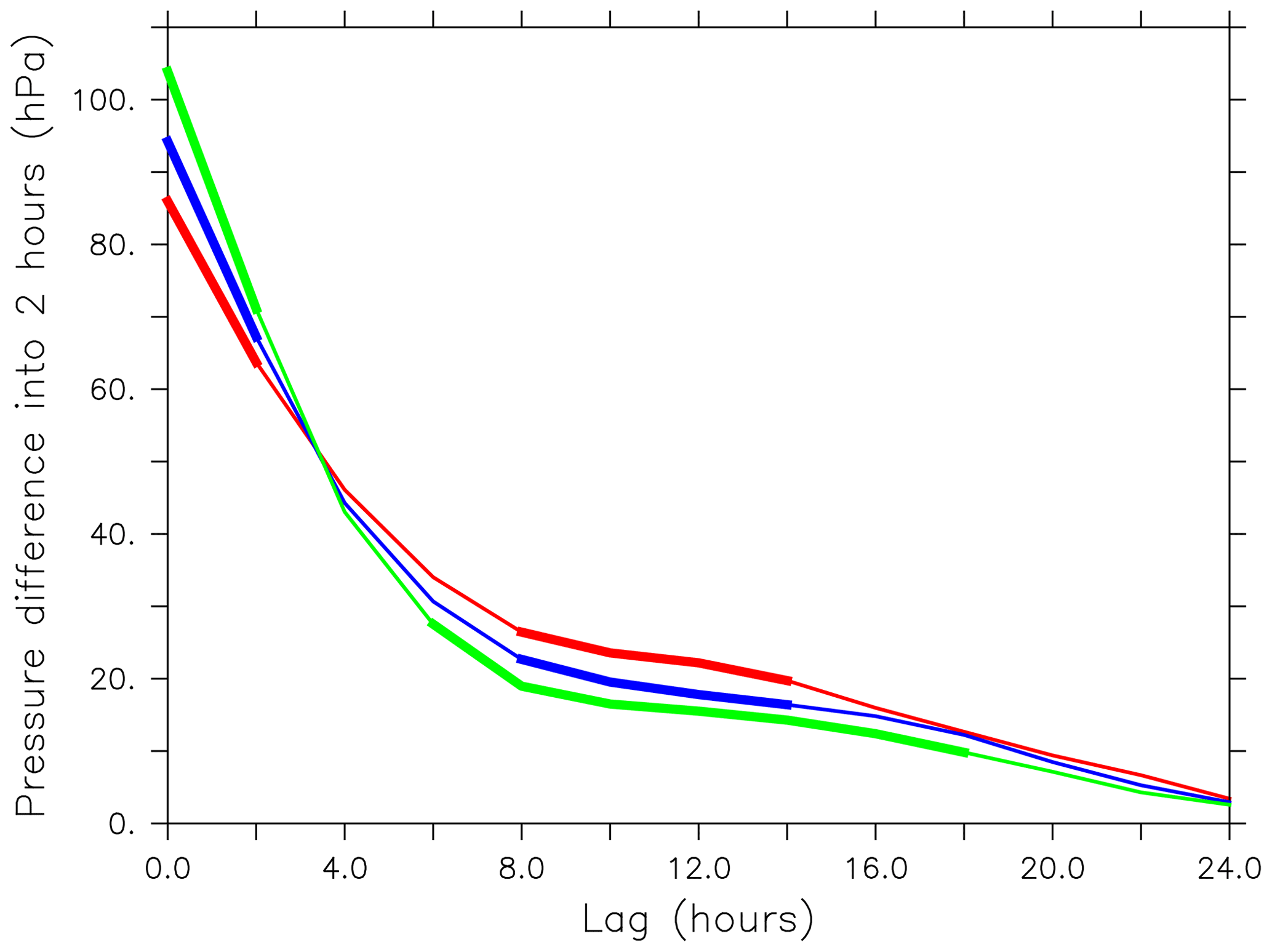
Figure 4Time lag composite of the pressure difference in 2 h over WCB trajectories for B85 (red), PCMT (blue) and NoConv (green) simulations. The zero lag corresponds to the time of maximum pressure difference. Only WCB trajectories having their maximum pressure difference reached before 12:00 UTC on 2 October are considered to get the same number of trajectories at all time lags. Thick segments correspond to time lags for which each composite is significantly different from the other two composites at 99.9 % following a Welch test.
3.2 Differences in the rapid ascending trajectories during the first 12 h of the simulations
To better visualize the effect of parameterized deep convection on heating rates in physical space, horizontal maps and vertical cross sections are shown at 21:00 UTC on 1 October in Fig. 5. This time was chosen because it corresponds to large differences in the proportion of the most rapidly ascending trajectories (i.e. those exceeding 100 hPa ascent within 2 h) between the three runs (Fig. 2d). Only the positions of WCB trajectories belonging to this category are shown in Fig. 5. The cold and bent-back warm fronts bring strong similarities between the three runs. Additionally, heating rates are strong for all runs ahead of the cold front and in the vicinity of the bent-back warm front (upper left side of Fig. 5a, c, e). Not surprisingly all the positions of the most rapidly ascending trajectories at that time are located within these regions of strong heating rate. However, the largest differences between the three runs appear in the heating rates ahead of the cold front (42–52∘ N, 26–22∘ W) and not near the bent-back warm front (52–56∘ N, 34–30∘ W). Ahead of the cold front, NoConv is characterized by four regions of strong heating rates with a few degrees extent in latitude and longitude and whose peak values are beyond 3 K h−1. In the same area, PCMT shows similar peak values, but the heating rates are more homogeneously distributed along the WCB than NoConv. In contrast, the peak values for B85 are much weaker (no more than 2.4 K h−1), and the large values of the heating rate are even more homogeneously distributed than in PCMT.
Vertical cross sections of the heating rates averaged between 42 and 48∘ N – that is, ahead of the cold front – are shown in Fig. 5b, d and f. In that region, the heating rate is much stronger in NoConv and PCMT than in B85 over the whole tropospheric column. In NoConv, strong heating rates appear in the upper troposphere at pressure levels lower than 350 hPa that do not exist for the two runs with parameterized convection. This yields slightly lower isentropic levels in the upper troposphere for NoConv compared to the other two runs. However, it is worth mentioning there also exist regions where NoConv tends to get much smaller heating values ahead of the cold front than the other two runs (see for instance the area centred at 50∘ N, 22∘ W). These results show similar findings to those of Martinez-Alvarado and Plant (2014), who compared two runs with full and reduced parameterized convection.
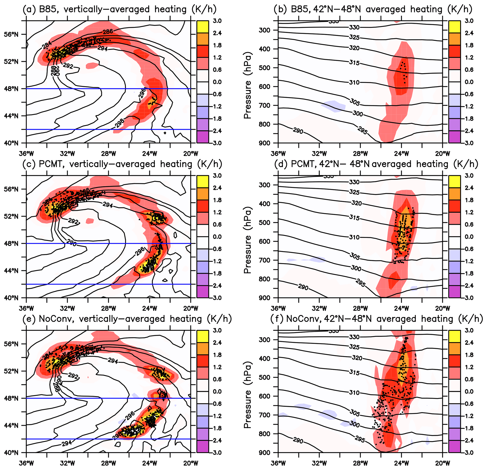
Figure 5(a, c, e) Vertically averaged heating rate between 300 and 800 hPa (shadings; units: K h−1), potential temperature at 850 hPa (interval: 2 K) and WCB trajectories satisfying 100 hPa ascent in 2 h at 21:00 UTC on 1 October for (a) B85, (c) PCMT and (e) NoConv simulations. (b, d, f) Latitudinally averaged (42–48∘ N; see blue lines in panels a, c and e) heating rate (shadings; units: K h−1), potential temperature (contours; interval: 5 K) and WCB trajectories satisfying 100 hPa ascent within 2 h and located in the same latitudinal band at 21:00 UTC on 1 October for (b) B85, (d) PCMT and (f) NoConv simulations.
3.3 Differences in the moderate ascending trajectories after 24 h simulations
Following Fig. 2d another particular interesting period is between 12:00 and 18:00 UTC on 2 October during which the proportion of trajectories with moderate ascents (25 hPa in 2 h) becomes much larger for B85 than the other two runs. Heating rates and trajectories having moderate ascents at 12:00 UTC on 2 October are shown in Fig. 6. Compared to 15 h earlier (Fig. 5), the peak values of the vertically averaged heating rates are weaker, and significant differences between the runs appear along the bent-back warm front. However, the qualitative picture is roughly the same. The NoConv heating rate is more bumpy along the front and marked by more pronounced regions of high and low heating rates than the other two runs. B85 is the run with smoother heating rate (Fig. 6a, c, e). There are two particular regions of inactivity in NoConv: one located along the front at 62∘ N, 26∘ W and another one further north between 63 and 65∘ N and from 32 to 24∘ W. PCMT exhibits slightly stronger heating rates and more trajectories with moderate ascents than NoConv in those regions. But B85 has an even stronger heating rate and many more trajectories. The difference in the number of trajectories seen in Fig. 2d mainly comes from these two regions.
Vertical cross sections of heating rates averaged between 63 and 65∘ N show that the second region of marked WCB inactivity in NoConv occurs at upper levels between 350 and 550 hPa in the longitudinal sector 34–24∘ W. We do see many more WCB trajectories with moderate ascents in B85 than in NoConv in association, with the heating rate peak values of the former being more than twice that of the latter (Fig. 6b, f). As already seen in Figs. 1–5, PCMT has an intermediate behaviour between B85 and NoConv (Fig. 6d). A decomposition of the heating rate into various physical processes shows that differences in the heating rates in that sector come from the resolved heating (sensible plus latent) and not the parameterized heating, which is mainly negligible at upper levels at that time (see Figs. S1 and S2). Parameterized convection and turbulence have similar amplitudes to the resolved heating in the lower troposphere but are negligible compared to the resolved heating at upper levels. The radiative term is found to be much smaller than the other terms in that sector at that time over the whole troposphere. Therefore it is not a direct effect of parameterized heating that is observed here but rather an indirect effect in which parameterized deep convection interacts with the resolved flow so that it leads to more intense WCB activity north of the front in the upper troposphere in B85 than in the other two runs.
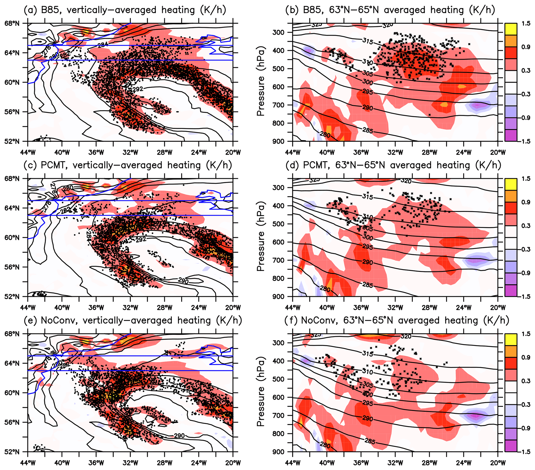
Figure 6(a, c, e) Vertically averaged heating rate between 300 and 800 hPa (shadings; units: K h−1), potential temperature at 850 hPa (interval: 2 K) and WCB trajectories satisfying 25 hPa ascent in 2 h at 12:00 UTC on 2 October for (a) B85, (c) PCMT and (e) NoConv simulations. (b, d, f) Latitudinally averaged (63–65∘ N; see blue lines in panels a, c and e) heating rate (shadings; units: K h−1), potential temperature (contours; interval: 5 K) and WCB trajectories satisfying 25 hPa ascent in 2 h and located in the same latitudinal band at 12:00 UTC on 2 October for (b) B85, (d) PCMT and (f) NoConv simulations.
Figure 7 provides a connection between the WCB activity, heating rates and PV patterns north of the front where large differences between the three runs have been identified. At lower pressure than 450 hPa, two main regions of WCB activity appear: one near 42–40∘ W in the vicinity of a well-marked localized negative PV region seen in all three runs (Fig. 7a, c, e) and another one along the band 34–24∘ W discussed previously. Areas of negative PV are visible slightly above and west of the latter region of WCB activity. These areas are small and centred at 32∘ W for PCMT and NoConv, whereas the area is much larger and extends from 36 to 32∘ W in B85. More WCB trajectories in B85 than in the other two runs would be a good explanation for the more extended negative PV area in B85. However, we observe that this negative PV area is not exactly co-located with the positions of the WCB trajectories which are a bit below and more to the east relative to the negative PV area (Fig. 7a). In other words, the PV loss undergone by WCB trajectories is not co-located with the negative PV area. To explain this shift of the negative PV area relative to the PV destruction region, it is important to consider spatial redistribution of PV by advection terms and in particular the indirect diabatic effects of advection by the divergent wind which tends to displace the PV destruction outward of the WCB outflow region (Archambault et al., 2013; Steinfeld and Pfahl, 2019). Ageostrophic winds that can be considered a proxy for the divergent winds are shown in Fig. 7b, d and f. West of the main WCB outflow region, i.e. west of 30∘ W in the 300–400 hPa layer, winds are westward and upward. Moving to the west they become more and more horizontal and align more with the isentropic slopes (compare the orientation of the vectors with the slope of the 315 K isentropic surface in Fig. 7a). The PV advection by the ageostrophic wind is generally negative because the stratospheric high PV values are west of the tropospheric low PV values. This leads to a westward expansion of the ridge anomaly, consistent with other studies (Steinfeld and Pfahl, 2019). Still looking at the same region, the ageostrophic winds are stronger in B85 than in PCMT or NoConv as expected from its more intense WCB activity there. While the advection terms are similar between the three runs between 44 and 40∘ W, they significantly differ between 38 and 36∘ W, where negative PV advection is clearly stronger for B85. Therefore, stronger WCB activity in connection with the higher heating rate in the middle and upper troposphere leads to stronger PV loss in the WCB outflow region in B85 compared to the other two runs, which is then advected upward and westward by the stronger divergent winds to form a more important zone of negative PV for the former run.
The findings of this section can be summarized as follows. With parameterized deep convection, heating rates are more homogeneously distributed along the cold and warm fronts, while without parameterized deep convection, heating rates are marked by strong spatial variations along the fronts. This leads to more rapid instantaneous ascents for the latter and more moderate but more sustained ascents for the former. Martinez-Alvarado and Plant (2014) also emphasized the smooth and regulating effect of parameterized deep convection within WCB. This is due to the fact that parameterized convection releases convective instability at subgrid scales, while explicit convection releases convective instability at resolved scales. Among the two schemes, B85 is the one having the greatest difference with NoConv, while PCMT has a more intermediate behaviour. The three runs significantly differ in terms of the impact of WCB activity on PV. The B85 scheme generally leads to higher heating rates at upper levels and more PV destruction in the upper troposphere during the second half of the simulations.
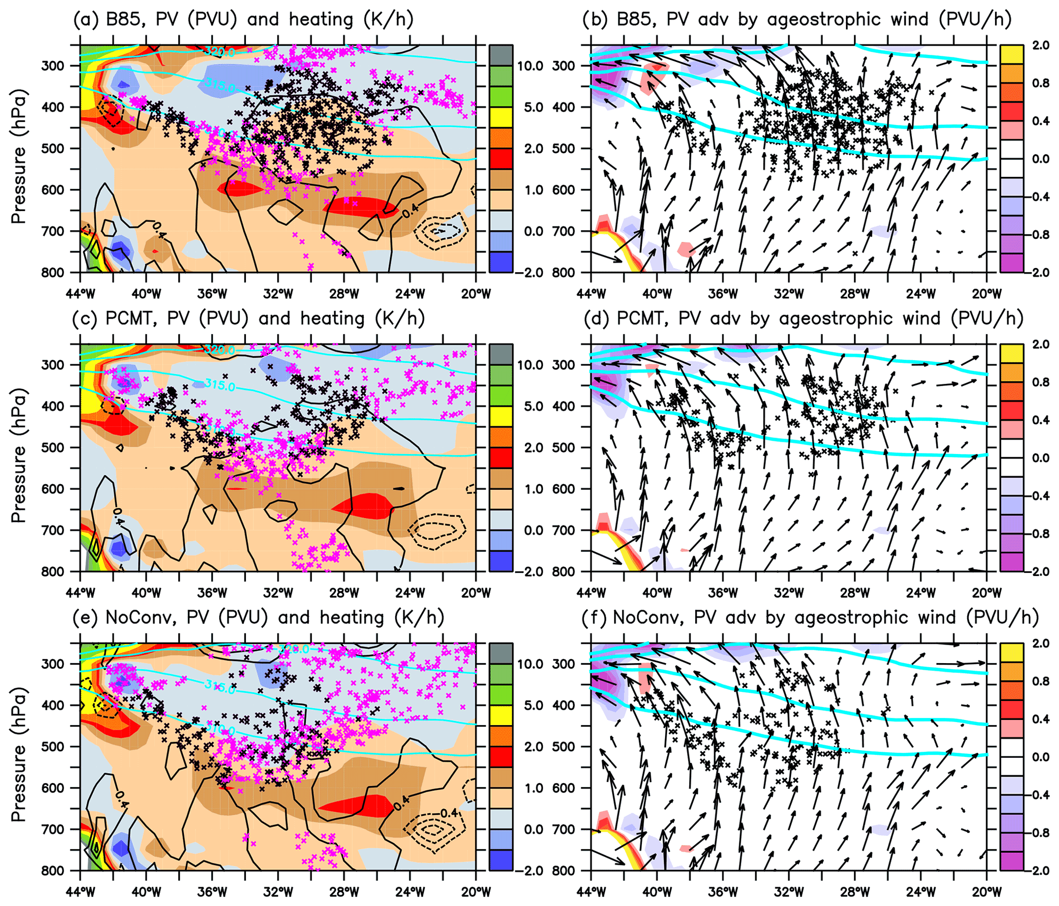
Figure 7(a, c, e) Latitudinally averaged (63–65∘ N) PV (shadings; units: PVU), heating rate (black contours; interval: 0.4 K h−1), potential temperature (light blue contours for 310, 315, 320 and 325 K) and WCB trajectories satisfying 25 hPa ascent in 2 h (black crosses) and the other WCB trajectories (purple crosses) and located in the same latitudinal band at 12:00 UTC on 2 October for (a) B85, (c) PCMT and (e) NoConv simulations. (b, d, f) Latitudinally averaged (63–65∘ N) PV advection by the zonal and vertical components of the ageostrophic wind (shadings; units: PVU h−1), and the associated ageostrophic wind vectors (black arrows). The light blue contours represent potential temperature as in left panels. The ageostrophic wind vectors are represented by multiplying respectively the zonal and vertical components by the distances occupied by 1 m in longitude and 1 Pa in pressure on the diagram.
The impact on the jet stream is investigated in the present section, and forecast skills of the three runs are assessed by comparing to the reanalyses and airborne observations.
4.1 Comparison to (re)analyses
PV horizontal maps at 300 hPa are shown for the three runs in Fig. 8 and compared with ECMWF-IFS and ARPEGE analyses and the ERA5 reanalysis. The separation between stratospheric and tropospheric air is well marked in all panels by an abrupt jump in PV from near zero and negative values to large positive values close to 8–10 PVU. This boundary is associated with a tropopause fold as shown in Fig. 7a, c and e. Despite this well-defined limit being located more or less at the same place for the six datasets (three simulations, two analyses and one reanalysis), the region of ridge building is not characterized by homogeneously distributed weak and negative PV values. For instance, at 64∘ N, going from 45 to 25∘ W (i.e. roughly along the main legs of the two Falcon flights), B85 exhibits large positive PV associated with stratospheric air, a sudden decrease to slightly negative values, then another area of positive PV values and finally negative values (Figs. 7a and 8d). The area of positive PV within the ridge forms a band of PV with values varying between 0.5 and 1.5 PVU largely covering the Greenland eastern coast (Fig. 8d) but whose vertical extent is rather limited between 300 and 350 hPa at 39∘ W (Fig. 7a). A similar narrow band of positive PV exists in the other datasets but with different values of PV and different locations. In the ECMWF-IFS analysis and ERA5, the positive PV values are smaller but have the same location as in B85 (Fig. 8a, c). In the ARPEGE analysis, the band is rather similar in intensity and location to B85, but this is not surprising since the ARPEGE analysis is made using a deterministic forecast whose deep convection scheme is B85. In contrast, in NoConv the band is eastward shifted by a few degrees in longitude compared to B85 (Figs. 7e and 8f). In PCMT, the band is less well defined, and the pattern resembles a mix between those of B85 and NoConv patterns.
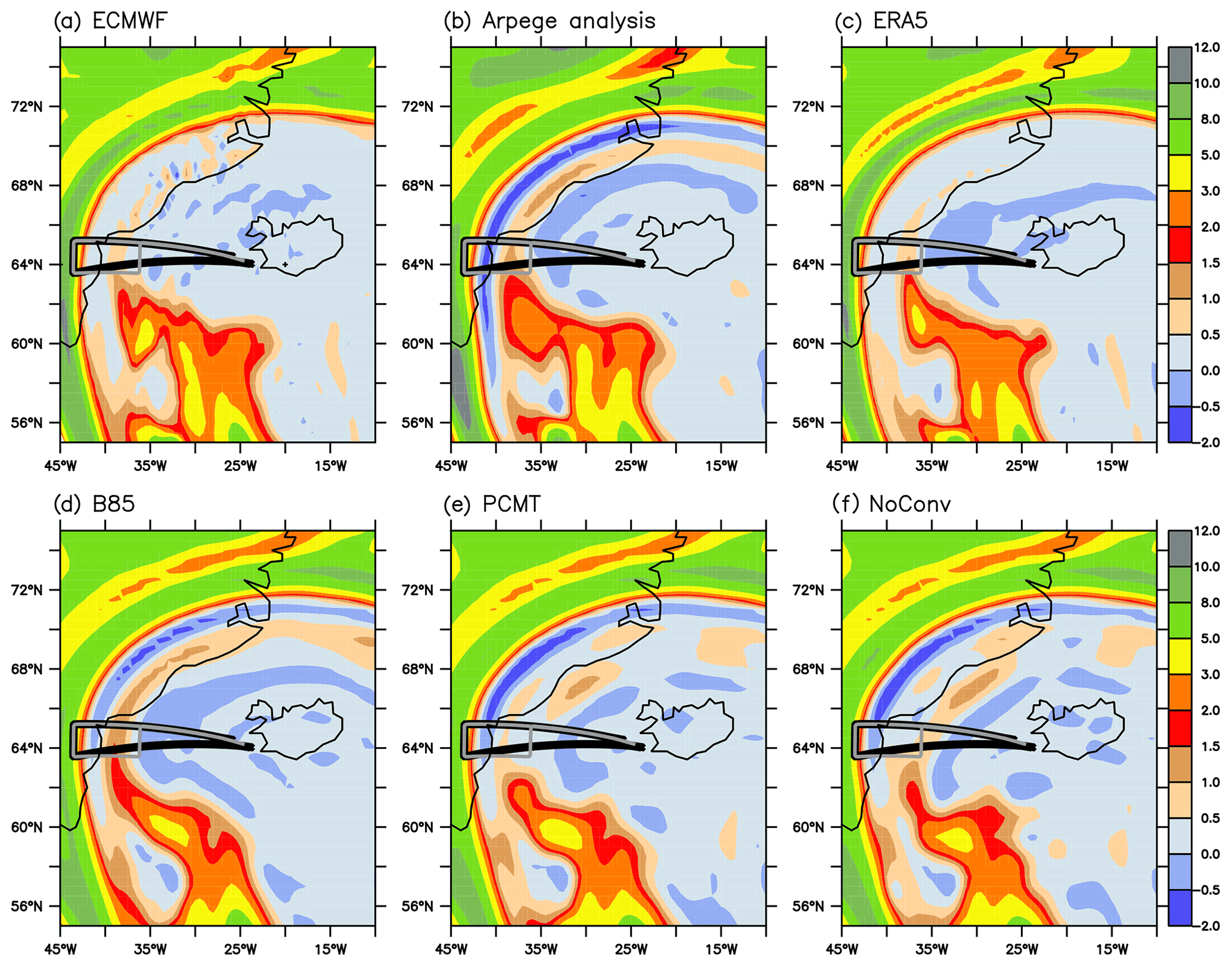
Figure 8Potential vorticity (units: PVU) at 300 hPa at 12:00 UTC on 2 October for the (a) ECMWF-IFS operational analysis, (b) ARPEGE operational analysis, (c) ERA5 reanalysis, (d) B85 run, (e) PCMT run and (f) NoConv run. The black and grey lines correspond to the SAFIRE and DLR Falcon flights that occurred between 09:00 and 12:00 UTC on 2 October in an anticlockwise direction.
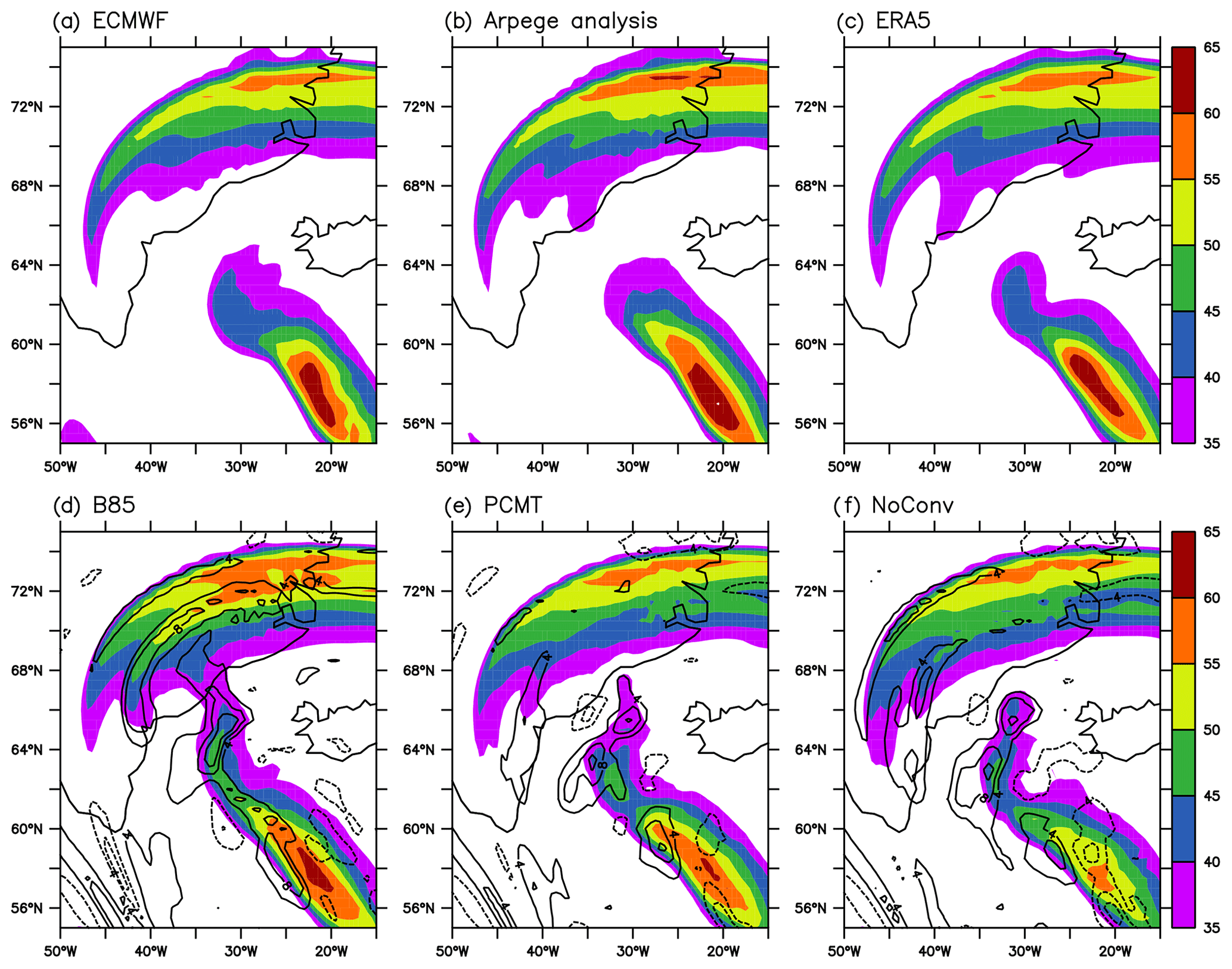
Because there are two jumps in PV at 300 hPa, a double jet structure is well visible in Fig. 9 for all datasets, with the main jet being the one more to the northwest separating the tropospheric air from the stratospheric air. While the secondary jet lies just above the Greenland eastern coastline for ECMWF-IFS, ARPEGE analyses, ERA5 and B85 (Fig. 9a–d), it is located further east in PCMT and NoConv (Fig. 9e–f). This is consistent with the PV gradient deduced from Fig. 8. In the immediate vicinity of the eastern coast of Greenland north of 64∘ N, PV values are higher to the west and lower to the east in ECMWF-IFS, ARPEGE analyses, ERA5 and B85, which explains the co-location of the secondary jet for these datasets. Anomalies with respect to the ECMWF-IFS analysis are shown in black contours in Fig. 9d–f. The B85 run produces a jet that is slightly too strong with positive anomalies of 4 m s−1 amplitude (Fig. 9d), consistent with the higher PV values along the narrow ribbon of 0.5–1.5 PVU values shown in Fig. 8d compared to ECMWF (Fig. 8b). The other two runs are marked by an eastward shift of the jet and negative anomalies of the order of 8 m s−1 amplitude over the Greenland eastern coastline (Fig. 9e–f), consistent with the eastward shift of the ribbon of 0.5–1.5 PVU values compared to the other datasets. At that time, B85 performs better than PCMT or NoConv in capturing the distance between the two jets, and this is attributed to the more active WCB in that region in B85 that reinforces the PV gradient further west and pushes the secondary jet closer to the main one. Another interesting feature is the stronger wind magnitude of the main jet in PCMT and NoConv compared to B85. This is due to more negative PV values just east of the tropopause fold (Fig. 8d–f) and more active WCB in that area for the former runs than the latter (see 42∘ W in Fig. 7a, c and e). Here, B85 is also slightly closer to ECMWF-IFS than the other two runs. In other words, the WCB outflow region is separated into two branches: one reinforcing the main jet and the other one the secondary jet. The runs are distinguished from each other in the relative importance of the two branches.
Six hours later, at 18:00 UTC on 2 October, the double jet structure is much less pronounced in ECMWF-IFS, ARPEGE analyses and ERA5 as well as in PCMT and NoConv, but it is still there in B85 (Fig. 10). Furthermore, the anomalies with respect to ECMWF-IFS are larger north of 64∘ N in B85 than PCMT or NoConv. In that case, B85 does not perform better than the other two runs and is even less skilful. Further south, the jet stream is too weak in NoConv compared to the other datasets (see the lower right side of the panels in Fig.10d–f), but this sector is not the focus of the present study as no flights were conducted there.

Figure 9Wind speed (shadings; units: m s−1) at 300 hPa at 12:00 UTC on 2 October for the (a) ECMWF-IFS operational analysis, (b) ARPEGE operational analysis, (c) ERA5 reanalysis, (d) B85 run, (e) PCMT run and (f) NoConv run. In panels (d)–(f), the black contours represent the wind speed anomalies (interval: 4 m s−1) of the three runs with respect to the ECMWF-IFS operational analysis. The black and grey lines correspond to the SAFIRE and DLR Falcon flights that occurred between 09:00 and 12:00 UTC on 2 October in an anticlockwise direction.
4.2 Comparison to airborne observations
For the flights of the two aircraft occurring in the region of the double jet structure (Fig. 9), it is worth comparing the three forecasts to airborne observations to determine which one performs better in representing the jet stream structure and intensity. The two aircraft followed each other with 10 min lag and observed the same meteorological features during more than half of the flights' duration. Besides, since the Doppler radar on board the SAFIRE Falcon and the Doppler lidar on board the DLR falcon are not sensitive to the same particles of the atmosphere, they provide complementary datasets as seen in Fig. 11a and b. The data have been interpolated at the model grid in the present study (Sect. 2.3.2), while higher-resolution profiles of the same datasets are shown in Fig. 9 of Schäfler et al. (2018).
In Fig. 11a, a good correspondence generally appears between the three kinds of measurements: Doppler radar, airborne in situ and the nine dropsondes. The intensities of the lower- and upper-level jets detected close to the Greenland coastline are similar in the dropsondes and radar data. The three datasets also agree on the intensities of the upper-level wind magnitude; two main regions of high values are distinguishable: one between 9.5 and 9.7 h and the other between 9.8 and 10 h. Some local discrepancies also occur for instance between the dropsonde data and radar data at 10.1 h or between the dropsonde data and in situ aircraft measurements at 10.5 h. The presence of a double jet structure is confirmed by the lidar measurements of the DLR Falcon (Fig. 11b), with the two jets being quite close to each other.
Figure 11c–e show the wind magnitude of the three forecasts. The double jet structure is present in all three runs as already shown in Fig. 9, but once again we do see that the distance between the two jets is significantly larger for PCMT and NoConv than B85. B85 is the forecast with the closest patterns to the observations, even though the distance between the two jets is still slightly too large in that run (e.g. compare Fig. 11b and c).
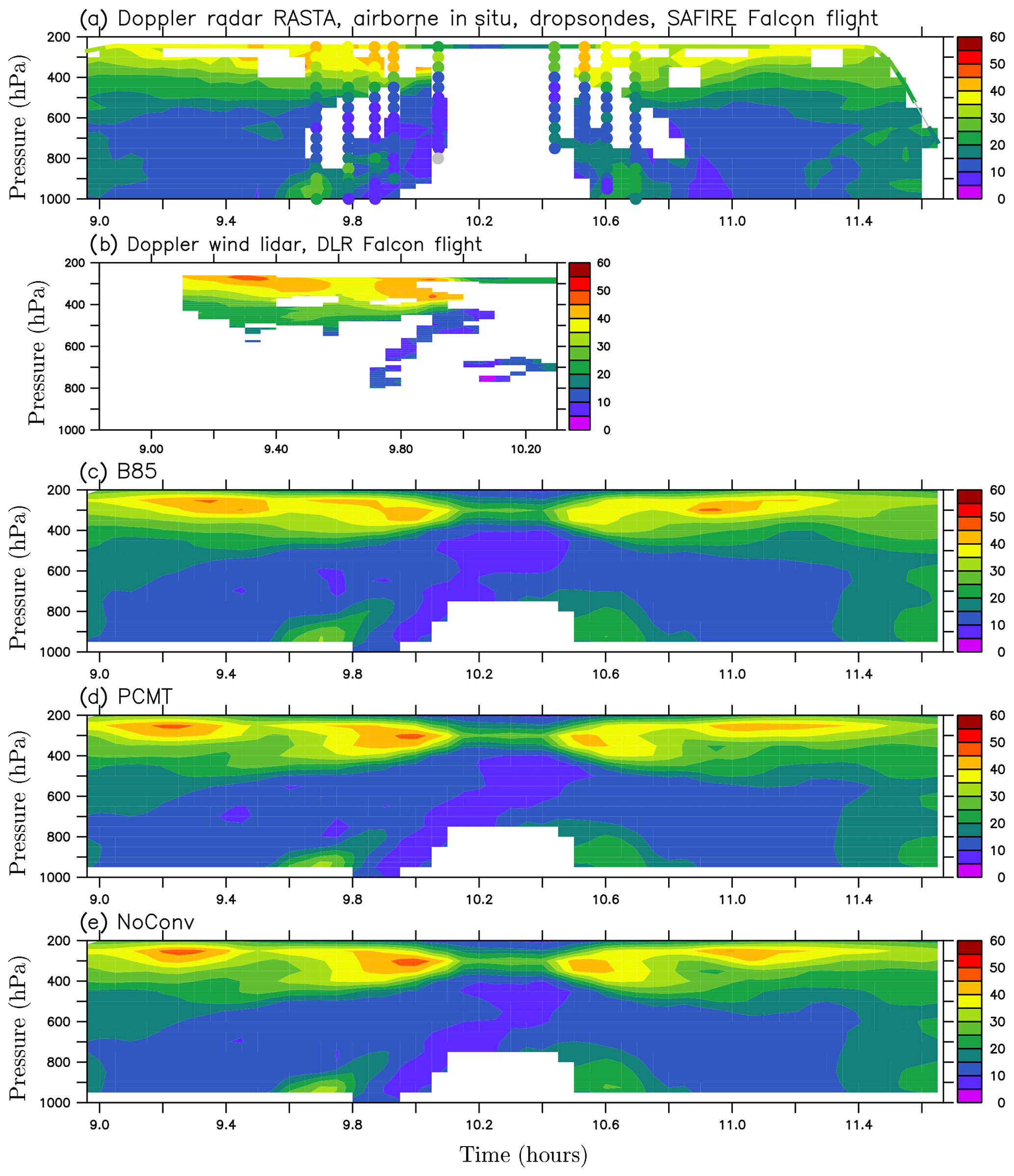
Figure 11Wind speed (units: m s−1) as function of time: (a) derived from the SAFIRE Falcon Doppler radar RASTA, airborne in situ measurements (upper coloured line) and dropsondes (coloured circles) along the whole flight track; (b) derived from the DLR Falcon 2 µm Doppler wind lidar along part of the flight common to the SAFIRE flight; and derived from (c) B85, (d) PCMT and (e) NoConv runs along the SAFIRE flight track. In panels (a) and (b), the measured wind speeds have been interpolated on the model grid. Note that all the panels can be compared to each other and the position and span of panel (b) are precisely chosen to have co-location in space with the other panels. The difference in time is there because the DLR Falcon was ahead of the SAFIRE Falcon with roughly a 20 min lag. In panels (c)–(e), the wind speed data are derived from 15 min output centred on the time of interest, which is that of the SAFIRE Falcon flight. See Sect. 2.3.2 for further details on the interpolations procedure.
To better visualize differences between forecasts and observations, forecast errors with respect to the observations made during the SAFIRE Falcon flight are shown in Fig. 12. While the three forecasts share the same errors at low levels with a too strong low-level jet in the vicinity of Greenland (see near 9.8 and 10.6 h), errors in the upper troposphere do not have the same magnitude among the three forecasts. Between 200 and 400 hPa, PCMT and NoConv forecast errors exhibit tripolar anomalies (positive–negative–positive) between 9.2 and 9.9 h and between 10.7 and 11.1 h, and their magnitude is about 12 m s−1. The negative forecast errors shown at 9.4 and 10.9 h are consistent with the negative anomalies shown in Fig. 9e and f in which the reference is the ECMWF-IFS analysis. In contrast, B85 errors fluctuate between 6 and 9 m s−1 only. The root-mean-square error computed in the upper troposphere (pressure lower than 500 hPa) for the difference between each run and the radar observations is 4.36 m s−1 for B85, 5.00 m s−1 for PCMT and 4.81 m s−1 for NoConv. Doing the same computation but using in situ airborne measurements, we get 4.27 m s−1 for B85, 5.43 m s−1 for PCMT and 5.65 m s−1 for NoConv, corresponding to an improvement of 10 % to 30 % in the representation of the wind speed in that region in B85 compared to the other two runs. To conclude, comparison with airborne observations confirms that B85 performs better than the other two forecasts in the location of the jets at 24 h lead time.
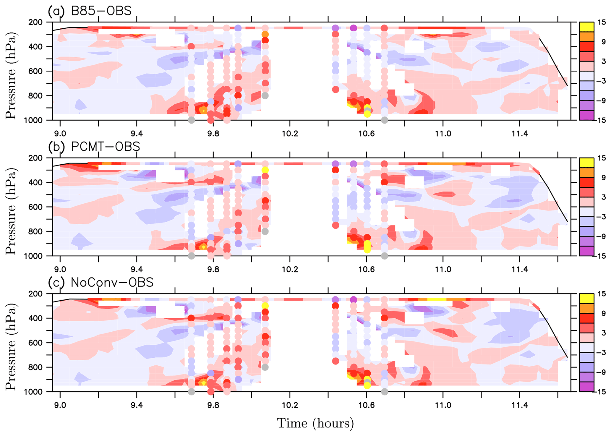
Figure 12Difference (experiment − observations) in wind speed (units: m s−1) for (a) B85, (b) PCMT and (c) NoConv simulations. The wind observations are composed of dropsondes, airborne in situ measurements and Doppler radar measurements along the SAFIRE Falcon track.
The effect of parameterized deep convection on WCB activity and jet stream was investigated by performing simulations of an explosively developing large-scale cyclone, which occurred from 29 September to 3 October 2016 during NAWDEX and is called the Stalactite cyclone, using the Météo-France global atmospheric model ARPEGE. Three simulations differing only from their deep convection representation are analysed. For two of them, parameterized deep convection was activated with distinct schemes (B85 corresponding to the Bougeault, 1985, scheme and PCMT corresponding to the Piriou et al., 2007, scheme), while for the third one, parameterized convection was turned off. The main findings can be summarized as follows and correspond to answers to the three main questions raised in the introduction.
-
How different are WCBs between simulations with active parameterized deep convection and those without? When the parameterized deep convection scheme is turned off, convective instability is released at the resolved scales such that few localized cells of a few degrees extent in longitude and latitude appear along the cold and warm fronts of the cyclone. These localized cells are characterized by strong heating and fast ascending motion. In contrast, when parameterized deep convection is active, the heating rate is more homogeneously distributed along the fronts, and its large values are more spread out while having weaker maxima than when deep convection is explicit at the model grid scales. This results in different behaviours in WCB ascents: without parameterized deep convection, ascents are rapid and abrupt, while with parameterized deep convection, ascents are more moderate but more sustained. These results confirm the regulating effect of parameterized deep convection emphasized by Martinez-Alvarado and Plant (2014).
-
What is the impact of parameterized deep convection on the jet stream at short range (less than 2 d)? Explicit convection yields strong localized heating over the whole troposphere that may potentially have a more important impact on the upper-level circulation locally than parameterized deep convection. However, the heating rate averaged over all WCB trajectories was found to be weaker for explicit deep convection than parameterized deep convection. Moreover, between 1 and 2 d lead times, one of the schemes (B85) shows more important averaged heating in the upper troposphere and more important vertical gradients of heating that lead to more PV destruction. This stronger heating can be attributed to the resolved heating and not the parameterized heating which is mainly localized at lower levels. These results should be contrasted with Done et al. (2006), who found that explicit convection yielded more PV destruction than parameterized convection in their case study. The present results also show that differences in WCB activity between explicit and parameterized deep convection may lead to large differences in the jet stream position and intensity at 1 d lead time. This is to be contrasted with Martinez-Alvarado and Plant (2014), who found rather modest impacts at the same short range. The impact on the upper-tropospheric circulation may depend on case studies. Here the extratropical cyclone is deeper that the one studied by Martinez-Alvarado and Plant (2014).
-
How different are WCBs and their impact on the jet stream between simulations performed with distinct deep convection schemes? The effects of the two deep convection schemes on WCB and their impact on the jet stream significantly differ from each other. B85 is the scheme inducing the most drastic differences compared to the run with explicit deep convection, while PCMT has a more intermediate behaviour. In terms of the impact on the jet stream, PCMT is closer to the run with explicit deep convection than to B85. Comparison with operational analyses and airborne observations of different types helped us to unambiguously determine the most skilful forecasts. At 1 d lead time, B85 performed better than the other two runs to represent the double jet structure. The shorter distance between the main and secondary jets in B85 than in other two forecasts was found to be more realistic by comparing to airborne observations and (re)analysis datasets. This was attributed to a more active branch of the WCB in a region of the upper troposphere that pushed the secondary jet closer to the main one. However, at the longer forecast range, this more active branch of the WCB was too strong and led to less realistic behaviour in B85 than the other two runs.
An analysis of the jet stream representation by the other members of the ARPEGE EPS shows that members 1, 2, 4, 5 and 9 behave similarly to member 0, which is the B85 run discussed in the present study (Fig. S3). All these members share the same deep convection scheme as B85 while they differ in the representation of other processes such as turbulence, shallow convection or oceanic flux. In contrast, members 3, 6, 7 and 8 resemble each other and are marked by a larger distance between the two jets than for the other set of members. The deep convection scheme of members 6, 7 and 8 is PCMT, while that of member 3 is the B85 scheme in which the humidity convergence closure was replaced by the CAPE closure. Since PCMT is also based on the CAPE closure, it indicates that the main difference in the jet representation between PCMT and B85 largely comes from the closure.
The humidity flux convergence used by the B85 closure has two components: one coming from the resolved-scale horizontal fluxes and the other from turbulent fluxes. The resolved-scale fluxes are expected to be strong in the presence of synoptic-scale forcing, like in the inflow regions of the warm conveyor belts. Therefore, it is not surprising to get more triggered convection in such cases with strong synoptic-scale forcing, when the closure is based on moisture convergence rather than when it is based on CAPE (PCMT convection scheme). In pure convective situations, when there is no significant synoptic-scale forcing, as for instance during summertime convection over land, CAPE is expected to get higher values, and in that case convection is less sensitive to humidity convergence (Yano et al., 2013).
Further investigations would be needed to better estimate the role of the convective closure type (such as CAPE closures versus moisture convergence closures) on the difference in cyclogenesis, WCB and jet stream dynamics. One way would be to analyse the mirror experiment – that is, PCMT closed with moisture convergence. The other way would be to run the B85 scheme by arbitrarily multiplying the intensity of the humidity convergence by a given factor in the closure, to investigate the sensitivity of WCB to convective intensity in the different regions of the WCB. These sensitivity experiments would necessitate a full analysis and could be an interesting aspect to investigate in future studies.
The sensitivity to initial conditions was analysed to check the robustness of the results. Starting the simulations 12 h earlier leads to similar findings: a too large distance between the two jets and a weaker secondary jet for PCMT compared to B85 (not shown). For hindcasts starting at even earlier dates (e.g. 30 September), members share similar forecast errors in the representation of the jet stream, and it is more difficult to state which one performs better, but we still observe a more intense secondary jet in B85.
Similar numerical simulations of the subsequent cyclone that followed the Stalactite cyclone 2 d after have been also analysed (IOP7; Schäfler et al., 2018). In that case, generation of negative PV at the tropopause level was found to be more pronounced in B85 than PCMT, leading to a stronger jet in the former than in the latter. The intermediate case based on the B85 scheme but activated with the CAPE closure resembles simulations based on the PCMT scheme (not shown). These results corroborate the case study of the Stalactite cyclone and support the idea that WCB in B85 is on average more active in the upper troposphere in connection with the humidity convergence closure.
While the focus of the present study was on the impact of parameterized deep convection in the WCB outflow region and horizontal structure of the jet stream, a companion paper will follow up to provide a more detailed analysis on the effect of parameterized deep convection in the ascending branch of the WCB and the vertical structure of the jet stream (Wimmer et al., 2021). It will rely on observations made during the second flight of the SAFIRE Falcon on 2 October, which were not shown here.
Data are available by contacting the corresponding author. ERA5 data are accessible via the climate data store (https://doi.org/10.24381/cds.bd0915c6, Hersbach et al., 2018).
The supplement related to this article is available online at: https://doi.org/10.5194/wcd-2-1011-2021-supplement.
GR and PA designed the initial study. GR and MW performed the data analysis, MW computed the Lagrangian trajectories and GR made the figures. CL performed the ARPEGE simulations with the help of JMP. PA developed the Lagrangian trajectory algorithm. JD, QC and JP provided the observational datasets. All authors contributed to the scientific discussions.
Some authors are members of the editorial board of Weather and Climate Dynamics. The peer-review process was guided by an independent editor, and the authors have also no other competing interests to declare.
Publisher’s note: Copernicus Publications remains neutral with regard to jurisdictional claims in published maps and institutional affiliations.
The authors thank the German Aerospace Center (Deutsches Zentrum für Luft- und Raumfahrt e.V., DLR) and Andreas Schäfler in particular for granting access to the DLR Falcon wind lidar data. The study benefited from discussions with the participants of the DIP-NAWDEX (Diabatic Processes in the North Atlantic Waveguide and Downstream impact Experiment) project, which is supported and funded by the Agence Nationale de la Recherche (ANR). It also benefited from discussions with our international NAWDEX partners during annual workshops. We thank Heini Wernli for downloading the ECMWF-IFS operational analysis data and Hanin Binder for sending them to us and for fruitful discussions on warm conveyor belts. Finally, two anonymous referees are acknowledged for their helpful comments during the review process.
This research has been supported by the Agence Nationale de la Recherche (grant no. ANR-17-CE01-0010-01). The airborne measurements and the SAFIRE Falcon flights received direct funding from IPSL, Météo-France, INSU-LEFE, EUFAR-NEAREX and ESA (EPATAN, contract no. 4000119015/16/NL/CT/gp). The DLR Falcon contribution to NAWDEX was supported by DLR, the European Space Agency (ESA, contract no. 4000114053/15/NL/FF/gp), NRL Monterrey and the EUropean Facility for Airborne Research (EUFAR, project NAWDEX Influence).
This paper was edited by Juliane Schwendike and reviewed by two anonymous referees.
Archambault, H. M., Bosart, L. F., Keyser, D., and Cordeira, J. M.: A Climatological Analysis of the Extratropical Flow Response to Recurving Western North Pacific Tropical Cyclones, Mon. Weather Rev., 141, 2325–2346, https://doi.org/10.1175/MWR-D-12-00257.1, 2013. a
Bauer, P., Thorpe, A., and Brunet, G.: The quiet revolution of numerical weather prediction, Nature, 525, 47–55, https://doi.org/10.1038/nature14956, 2015. a
Baumgart, M., Riemer, M., Wirth, V., and Teubler, F.: Potential Vorticity Dynamics of Forecast Errors: A Quantitative Case Study, Mon. Weather Rev., 146, 1405–1425, https://doi.org/10.1175/MWR-D-17-0196.1, 2018. a
Bechtold, P., Bazile, E., Guichard, F., Mascart, P., and Richard, E.: A mass flux convection scheme for regional and global models, Q. J. Roy. Meteor. Soc., 127, 869–886, https://doi.org/10.1002/qj.49712757309, 2001. a, b
Belamari, S.: Report on uncertainty estimates of an optimal bulk formulation for surface turbulent fluxes, (Deliverable No. D.4.1.2), Toulouse, France, Marine environment and security for the European area – Integrated Project (MERSEA IP), 2005. a, b
Binder, H., Boettcher, M., Joos, H., and Wernli, H.: The Role of Warm Conveyor Belts for the Intensification of Extratropical Cyclones in Northern Hemisphere Winter, J. Atmos. Sci., 73, 3997–4020, https://doi.org/10.1175/JAS-D-15-0302.1, 2016. a
Binder, H., Rivière, G., Arbogast, P., Maynard, K., Bosser, P., Joly, B., and Labadie, C.: Dynamics of forecast-error growth along cut-off Sanchez and its consequence for the prediction of a high-impact weather event over southern France, Q. J. Roy. Meteor. Soc., 147, 3263–3285, https://doi.org/10.1002/qj.4127, 2021. a
Blanchard, N., Pantillon, F., Chaboureau, J. P., and Delanoë, J.: Organization of convective ascents in a warm conveyor belt, Weather Clim. Dynam., 1, 617–634, https://doi.org/10.5194/wcd-1-617-2020, 2020. a, b, c, d
Blanchard, N., Pantillon, F., Chaboureau, J. P., and Delanoë, J.: Mid-level convection in a warm conveyor belt accelerates the jet stream, Weather Clim. Dynam., 2, 37–53, https://doi.org/10.5194/wcd-2-37-2021, 2021. a, b, c, d
Booth, J. F., Naud, C. M., and Willison, J.: Evaluation of extratropical cyclone precipitation in the North Atlantic Basin: An analysis of ERA-Interim, WRF, and two CMIP5 models, J. Climate, 31, 2345–2360, https://doi.org/10.1175/JCLI-D-17-0308.1, 2018. a
Bougeault, P.: A simple parameterization of the large-scale effects of cumulus convection., Mon. Weather Rev., 113, 2105–2121, 1985. a, b, c, d
Bouteloup, Y., Seity, Y., and Bazile, E.: Description of the sedimentation scheme used operationally in all Météo-France NWP models, Tellus A, 63, 300–311, https://doi.org/10.1111/j.1600-0870.2010.00484.x, 2011. a
Browning, K. A.: Organization of clouds and precipitation in extratropical cyclones, vol. : extratropical cyclones, Erik Palmén memorial volume, chap. 8, 129–153, American Meteorological Society, 1990. a
Chagnon, J., Gray, S. L., and Methven, J.: Diabatic processes modifying potential vorticity in a North Atlantic Cyclone, Q. J. Roy. Meteor. Soc., 139, 1270–1282, 2013. a
Courtier, P., Freydier, C., Geleyn, J., Rabier, F., and Rochas, M.: The ARPEGE project at Météo-France., in: ECMWF Seminar Proceedings, Reading, volume II, 193–231, 1991. a
Crespo, J. A. and Posselt, D. J.: A-Train-Based Case Study of Stratiform–Convective Transition within a Warm Conveyor Belt, Mon. Weather Rev., 144, 2069–2084, https://doi.org/10.1175/MWR-D-15-0435.1, 2016. a, b
Cuxart, J., Bougeault, P., and Redelsperger, J. L.: A Turbulence Scheme Allowing for Mesoscale and Large-Eddy Simulations., Q. J. Roy. Meteor. Soc., 126, 1–30, https://doi.org/10.1002/qj.49712656202, 2000. a, b
Delanoe, J., Protat, A., Jourdan, O., Pelon, J., Papazonni, M., Dupuy, R., Gayet, J.-F., and Jouan, C.: Comparison of Airborne In Situ, Airborne Radar-Lidar, and Spaceborne Radar-Lidar Retrievals of Polar Ice Cloud Properties Sampled during the POLARCAT Campaign, J. Atmos. Ocean. Tech., 30, 57–73, 2013. a
Descamps, L., Labadie, C., Joly, A., Bazile, E., Arbogast, P., and Cébron, P.: PEARP, the Météo-France short-range ensemble prediction system., Q. J. Roy. Meteor. Soc., 141, 1671–1685, 2015. a
Done, J. M., Craig, G. C., Gray, S. L., Clark, P. A., and Gray, M. E. B.: Mesoscale simulations of organized convection: Importance of convective equilibrium, Q. J. Roy. Meteor. Soc., 132, 737–756, 2006. a, b
Ducrocq, V. and Bougeault, P.: Simulations of an observed squall line with a meso-beta scale hydrostatic model, Weather Forecast., 10, 380–399, 1995. a
Ertel, H.: Ein neuer hydrodynamischer Wirbelsatz, Meteorol. Z., 59, 271–281, 1942. a
Flack, D. L. A., Rivière, G., Musat, I., Roehrig, R., Bony, S., Delanoë, J., Cazenave, Q., and Pelon, J.: Representation by two climate models of the dynamical and diabatic processes involved in the development of an explosively deepening cyclone during NAWDEX, Weather Clim. Dynam., 2, 233–253, https://doi.org/10.5194/wcd-2-233-2021, 2021. a, b
Flaounas, E., Lagouvardos, K., Kotroni, V., Claud, C., Delanoë, J., Flamant, C., Madonna, E., and Wernli, H.: Processes leading to heavy precipitation associated with two Mediterranean cyclones observed during the HyMeX SOP1, Q. J. Roy. Meteor. Soc., 142, 275–286, https://doi.org/10.1002/qj.2618, 2016. a, b
Flaounas, E., Kotroni, V., Lagouvardos, K., Gray, S. L., Rysman, J.-F., and Claud, C.: Heavy rainfall in Mediterranean cyclones. Part I: contribution of deep convection and warm conveyor belt, Clim. Dynam., 50, 2935–2949, https://doi.org/10.1007/s00382-017-3783-x, 2018. a, b
Grams, C. M., Wernli, H., Bottcher, M., Campa, J., Corsmeier, U., Jones, S. C., Keller, J. H., Lenz, C.-J., and Wiegand, L.: The key role of diabatic processes in modifying the upper-tropospheric wave guide: a North Atlantic case-study, Q. J. Roy. Meteor. Soc., 137, 2174–2193, https://doi.org/10.1002/qj.891, 2011. a
Grams, C. M., Magnusson, L., and Madonna, E.: An atmospheric dynamics perspective on the amplification and propagation of forecast error in numerical weather prediction models: a case study, Q. J. Roy. Meteor. Soc., 144, 2577–2591, https://doi.org/10.1002/qj.3353, 2018. a, b, c
Gray, S. L., Dunning, C. M., Methven, J., Masato, G., and Chagnon, J. M.: Systematic model forecast error in Rossby wave structure, Geophys. Res. Lett., 41, 2979–2987, 2014. a, b
Hersbach, H., Bell, B., Berrisford, P., Biavati, G., Horányi, A., Muñoz Sabater, J., Nicolas, J., Peubey, C., Radu, R., Rozum, I., Schepers, D., Simmons, A., Soci, C., Dee, D., and Thépaut, J.-N.: ERA5 hourly data on pressure levels from 1979 to present, Copernicus Climate Change Service (C3S) Climate Data Store (CDS) [data set], https://doi.org/10.24381/cds.bd0915c6, 2018. a
Hersbach, H., Bell, B., Berrisford, P., Hirahara, S., Horanyi, A., Munoz-Sabater, J., Nicolas, J., Peubey, C., Radu, R., Schepers, D., Simmons, A., Soci, C., Abdalla, S., Abellan, X., Balsamo, G., Bechtold, P., Biavati, G., Bidlot, J., Bonavita, M., Chiara, G. D., Dahlgren, P., Dee, D., Diamantakis, M., Dragani, R., Flemming, J., Forbes, R., Fuentes, M., Geer, A., Haimberger, L., Healy, S., Hogan, R. J., Hólm, E., Janisková, M., Keeley, S., Laloyaux, P., Lopez, P., Lupu, C., Radnoti, G., de Rosnay, P., Rozum, I., Vamborg, F., Villaume, S., and Thépaut, J.-N.: The ERA5 global reanalysis, Q. J. Roy. Meteor. Soc., 146, 1999–2049, https://doi.org/10.1002/qj.3803, 2020. a
Hewson, T., Magnusson, L., Breivik, O., Prates, F., Tsonevsky, I., and Vries, H. J. W. D.: Windstorms in northwest Europe in late 2013, ECMWF Newsletter, Spring 2014, 22–28, 2014. a
Jeyaratnam, J., Booth, J. F., Naud, C. M., Luo, Z. J., and Homeyer, C. R.: Upright convection in extratropical cyclones: A survey using ground based radar data over the United States., Geophys. Res. Lett., 47, e2019GL086620, https://doi.org/10.1029/2019GL086620, 2020. a, b
Joos, H. and Wernli, H.: Influence of microphysical processes on the potential vorticity development in a warm conveyor belt: a case-study with the limited-area model COSMO, Q. J. Roy. Meteor. Soc., 138, 407–418, https://doi.org/10.1002/qj.934, 2012. a
Kain, J. and Fritsch, J.: Convective Parameterization for Mesoscale Models: The Kain-Fritsch Scheme,, vol. The Representation of Cumulus Convection in Numerical Models of Meteorol. Monogr., chap. 16, 165–170, American Meteorological Society, Boston, MA, https://doi.org/10.1007/978-1-935704-13-3_16, 1993. a, b
Korfe, N. G. and Colle, B. A.: Evaluation of Cool-Season Extratropical Cyclones in a Multimodel Ensemble for Eastern North America and the Western Atlantic Ocean, Weather Forecast., 33, 109–127, https://doi.org/10.1175/WAF-D-17-0036.1, 2018. a
Kuo, H.: On formation and intensification of tropical cyclones through latent heat release by cumulus convection, J. Atmos. Sci., 22, 40–63, 1965. a
Lillo, S. P. and Parsons, D. B.: Investigating the dynamics of error growth in ECMWF medium-range forecast busts, Q. J. Roy. Meteor. Soc., 143, 1211–1226, https://doi.org/10.1002/qj.2938, 2017. a
Lopez, P.: Implementation and validation of a new prognostic large-scale cloud and precipitation scheme for climate and data-assimilation purposes, Q. J. Roy. Meteor. Soc., 128, 229–257, https://doi.org/10.1256/00359000260498879, 2002. a, b
Louis, J.: A parametric model of vertical eddy fluxes in the atmosphere, Bound.-Lay. Meteorol., 17, 187–202, https://doi.org/10.1007/BF00117978, 1979. a
Maddison, J. W., Gray, S. L., Martinez-Alvarado, O., and Williams, K. D.: Upstream cyclone influence on the predictability of block onsets over the Euro-Atlantic region, Mon. Weather Rev., 147, 1277–1296, https://doi.org/10.1175/MWR-D-18-0226.1, 2019. a
Maddison, J. W., Gray, S. L., Martinez-Alvarado, O., and Williams, K. D.: Impact of model upgrades on diabatic processes in extratropical cyclones and downstream forecast evolution, Q. J. Roy. Meteor. Soc., 146, 1322–1350, https://doi.org/10.1002/qj.3739, 2020. a, b, c, d, e
Madonna, E., Wernli, H., Joos, H., and Martius, O.: Warm Conveyor Belts in the ERA-Interim Dataset (1979–2010). Part I: Climatology and Potential Vorticity Evolution, J. Climate, 27, 3–26, https://doi.org/10.1175/JCLI-D-12-00720.1, 2014. a
Martinez-Alvarado, O. and Plant, R. S.: Parametrized diabatic processes in numerical simulations of an extratropical cyclone, Q. J. Roy. Meteor. Soc., 140, 1742–1755, https://doi.org/10.1002/qj.2254, 2014. a, b, c, d, e, f
Martinez-Alvarado, O., Baker, L. H., Gray, S. L., Methven, J., and Plant, R. S.: Distinguishing the Cold Conveyor Belt and Sting Jet Airstreams in an Intense Extratropical Cyclone, Mon. Weather Rev., 142, 2571–2595, 2014a. a
Martinez-Alvarado, O., Joos, H., Chagnon, J., Boettcher, M., Gray, S. L., Plant, R. S., Methven, J., and Wernli, H.: The dichotomous structure of the warm conveyor belt, Q. J. Roy. Meteor. Soc., 140, 1809–1824, 2014b. a
Martinez-Alvarado, O., Madonna, E., Gray, S., and Joos, H.: A route to systematic error in forecasts of Rossby waves, Q. J. Roy. Meteor. Soc., 142, 196–210, https://doi.org/10.1002/qj.2645, 2016. a
Mazoyer, M., Ricard, D., Rivière, G., Delanoë, J., Arbogast, P., Vié, B., Lac, C., Cazenave, Q., and Pelon, J.: Microphysics impacts on the warm conveyor belt and ridge building of the NAWDEX IOP6 cyclone, Mon. Weather Rev., https://doi.org/10.1175/MWR-D-21-0061.1, in press, 2021. a
Neiman, P., Shapiro, M., and Fedor, L.: The life cycle of an extratropical marine cyclone. Part II: Mesoscale structure and diagnostics, Mon. Weather Rev., 121, 2177–2199, 1993. a
Oertel, A., Boettcher, M., Joos, H., Sprenger, M., and Wernli, H.: Convective activity in an extratropical cyclone and its warm conveyor belt – a case-study combining observations and a convection-permitting model simulation, Q. J. Roy. Meteor. Soc., 145, 1406–1426, https://doi.org/10.1002/qj.3500, 2019. a, b, c
Oertel, A., Boettcher, M., Joos, H., Sprenger, M., and Wernli, H.: Potential vorticity structure of embedded convection in a warm conveyor belt and its relevance for large-scale dynamics, Weather Clim. Dynam., 1, 127–153, https://doi.org/10.5194/wcd-1-127-2020, 2020. a, b, c, d
Oertel, A., Sprenger, M., Joos, H., Boettcher, M., Konow, H., Hagen, M., and Wernli, H.: Observations and simulation of intense convection embedded in a warm conveyor belt – how ambient vertical wind shear determines the dynamical impact, Weather Clim. Dynam., 2, 89–110, https://doi.org/10.5194/wcd-2-89-2021, 2021. a, b
Pergaud, J., Masson, V., Malardel, S., and Couvreux, F.: A Parameterization of Dry Thermals and Shallow Cumuli for Mesoscale Numerical Weather Prediction, Bound.-Lay. Meteorol., 132, 83, https://doi.org/10.1007/s10546-009-9388-0, 2009. a
Piriou, J.-M., Redelsperger, J.-L., Geleyn, J.-F., Lafore, J.-P., and Guichard, F.: An approach for convective parameterization with memory: Separating microphysics and transport in grid-scale equations, J. Atmos. Sci., 64, 4127–4139, https://doi.org/10.1175/2007JAS2144.1, 2007. a, b, c, d, e
Pomroy, H. and Thorpe, A.: The evolution and dynamical role of reduced upper-tropospheric potential vorticity in intensive observing period one of FASTEX, Mon. Weather Rev., 128, 1817–1834, 2000. a
Ponzano, M., Joly, B., Descamps, L., and Arbogast, P.: Systematic error analysis of heavy-precipitation-event prediction using a 30-year hindcast dataset, Nat. Hazards Earth Syst. Sci., 20, 1369–1389, https://doi.org/10.5194/nhess-20-1369-2020, 2020. a, b
Rasp, S., Selz, T., and Craig, G. C.: Convective and Slantwise Trajectory Ascent in Convection-Permitting Simulations of Midlatitude Cyclones, Mon. Weather Rev., 144, 3961–3976, https://doi.org/10.1175/MWR-D-16-0112.1, 2016. a
Rodwell, M. J., Magnusson, L., and co authors: Characteristics of occasional poor medium-range weather forecasts for Europe, B. Am. Meteorol. Soc., 94, 1393–1405, 2013. a, b, c
Roehrig, R., Beau, I., Saint-Martin, D., Alias, A., Decharme, B., Guérémy, J.-F., Voldoire, A., Younous, A., Bazile, E., Belamari, S., Blein, S., Bouniol, D., Bouteloup, Y., Cattiaux, J., Chauvin, F., Chevallier, M., Colin, J., Douville, H., Marquet, P., Michou, M., Nabat, P., Oudar, T., Peyrillé, P., Piriou, J.-M., Salas y Melia, D., Séférian, R., and Sénési, S.: The CNRM global atmosphere model ARPEGE‐Climat 6.3: description and evaluation, J. Adv. Model. Earth Sy., 12, e2020MS002075, https://doi.org/10.1029/2020MS002075, 2020. a, b
Schäfler, A., Craig, G., Wernli, H., Arbogast, P., Doyle, J. D., McTaggart-Cowan, R., Methven, J., Rivière, G., Ament, F., Boettcher, M., Bramberger, M., Cazenave, Q., Cotton, R., Crewell, S., Delanoë, J., Dörnbrack, A., Ehrlich, A., Ewald, F., Fix, A., Grams, C. M., Gray, S. L., Grob, H., Groß, S., Hagen, M., Harvey, B., Hirsch, L., Jacob, M., Kölling, T., Konow, H., Lemmerz, C., Lux, O., Magnusson, L., Mayer, B., Mech, M., Moore, R., Pelon, J., Quinting, J., Rahm, S., Rapp, M., Rautenhaus, M., Reitebuch, O., Reynolds, C. A., Sodemann, H., Spengler, T., Vaughan, G., Wendisch, M., Wirth, M., Witschas, B., Wolf, K., and Zinner, T.: The North Atlantic Waveguide and Downstream Impact Experiment., B. Am. Meteorol. Soc., 99, 1607–1637, 2018. a, b, c, d
Schemm, S., Wernli, H., and Papritz, L.: Warm conveyor belt in idealized moist baroclinic wave simulation, J. Atmos. Sci., 70, 627–652, https://doi.org/10.1175/JAS-D-12-0147.1, 2013. a, b
Selz, T. and Craig, G.: Upscale Error Growth in a High-Resolution Simulation of a Summertime Weather Event over Europe, Mon. Weather Rev., 143, 813–827, https://doi.org/10.1175/MWR-D-14-00140.1, 2015. a
Simmons, A. and Hollingsworth, A.: Some aspects of the improvement in skill of numerical weather prediction, Q. J. Roy. Meteor. Soc., 128, 647–677, 2002. a
Steinfeld, D. and Pfahl, S.: The role of latent heating in atmospheric blocking dynamics: a global climatology, Clim. Dynam., 53, 6159–6180, https://doi.org/10.1007/s00382-019-04919-6, 2019. a, b
Stoelinga, M. T.: A Potential Vorticity-Based Study of the Role of Diabatic Heating and Friction in a Numerically Simulated Baroclinic Cyclone, Mon. Weather Rev., 124, 849–874, 1996. a
Tribbia, J. J. and Baumhefner, D. P.: The reliability of improvements in deterministic short-range forecasts in the presence of initial state and modeling deficiencies, Mon. Weather Rev., 116, 2276–2288, 1988. a
Weissmann, M., Busen, R., Dörnbrack, A., Rahm, S., , and Reitebuch, O.: Targeted observations with an airborne wind lidar, J. Atmos. Tech., 22, 1706–1719, 2005. a
Wernli, H. and Davies, H. C.: A Lagrangian-based analysis of extratropical cyclones. I: The method and some applications, Q. J. Roy. Meteor. Soc., 123, 467–489, 1997. a, b, c
Wimmer, M., Rivière, G., Arbogast, P., Piriou, J.-M., Delanoe, J., Labadie, C., Cazenave, Q., and Pelon, J.: Diabatic processes modulating the vertical structure of the jet stream: sensitivity to deep convection schemes, Weather Clim. Dynam., in preparation, 2021. a
Witschas, B., Rahm, S., Dörnbrack, A., Wagner, J., and Rapp, M.: Airborne wind lidar measurements of vertical and horizontal winds for the investigation of orographically induced gravity waves., J. Atmos. Ocean. Tech., 34, 1371–1386, https://doi.org/10.1175/JTECH-D-17-0021.1, 2017. a
Yano, J.-I., Bister, M., Fuchs, Ž., Gerard, L., Phillips, V. T. J., Barkidija, S., and Piriou, J.-M.: Phenomenology of convection-parameterization closure, Atmos. Chem. Phys., 13, 4111–4131, https://doi.org/10.5194/acp-13-4111-2013, 2013. a
Zhang, F., Bei, N., Rotunno, R., Snyder, C., and Epifanio, C.: Meso-scale predictability of moist baroclinic waves: Convection- permitting experiments and multistage error growth dynamics, J. Atmos. Sci., 64, 3579–3594, https://doi.org/10.1175/JAS4028.1, 2007. a
- Abstract
- Introduction
- Data and method
- Impact of convection representation on heating rates and warm conveyor belt trajectories
- Impact of deep convection representation on the jet stream
- Conclusions
- Data availability
- Author contributions
- Competing interests
- Disclaimer
- Acknowledgements
- Financial support
- Review statement
- References
- Supplement