The three-dimensional life cycles of potential vorticity cutoffs: a global and selected regional climatologies in ERA-Interim (1979–2018)

The aim of this study is to explore the nature of potential vorticity (PV) cutoff life cycles. While climatological frequencies of such near-tropopause cyclonic vortices are well known, their life cycle and in particular their three-dimensional evolution is poorly understood. To address this gap, a novel method is introduced that uses isentropic air parcel trajectories to track PV cutoffs as three-dimensional objects. With this method, we can distinguish the two fundamentally different PV cutoff lysis scenarios on isentropic surfaces: complete diabatic decay vs. reabsorption by the stratospheric reservoir. This method is applied to the ERA-Interim dataset (1979–2018), and the first global climatology of PV cutoffs is presented that is independent of the selection of a vertical level and identifies and tracks PV cutoffs as three-dimensional features. More than 150 000 PV cutoff life cycles are identified and analyzed. The climatology confirms known frequency maxima of PV cutoffs and identifies additional bands in subtropical areas in the summer hemispheres and a circumpolar band around Antarctica. The first climatological analysis of diabatic decay and reabsorption shows that both scenarios occur equally frequently – in contrast to the prevailing opinion that diabatic decay dominates. Then, PV cutoffs are classified according to their position relative to jet streams (equatorward (Type I), between two jets (Type II), and poleward (Type III)). A composite analysis shows distinct dynamical scenarios for the genesis of the three types. Type I forms due to anticyclonic Rossby wave breaking above subtropical surface anticyclones and hardly results in precipitation. Type II results from anticyclonic Rossby wave breaking in mid-latitudes in regions with split-jet conditions and is frequently accompanied by surface cyclogenesis and substantial precipitation. Type III cutoffs preferentially form due to cyclonic Rossby wave breaking within extratropical cyclones in the storm track regions. We show that important track characteristics (speed, travel distance, frequency of decay and reabsorption, isentropic levels) differ between the categories, while lifetime is similar in all categories. Finally, 12 PV cutoff genesis regions in DJF and JJA are selected to study the regional characteristics of PV cutoff life cycles. As a particularly novel aspect, the vertical evolution of PV cutoffs along the life cycle is investigated. We find that, climatologically, PV cutoffs reach their maximum vertical extent about one day after genesis in most regions. However, while in some regions PV cutoffs rapidly disappear at lower levels by diabatic decay, they can grow downward in other regions. In addition, regional differences in lifetimes, the frequencies of diabatic decay and reabsorption, and the link to surface cyclones are identified that cannot be explained only by the preferred regional occurrence of the different cutoff types as defined above. Finally, we also show that in many regions PV cutoffs can be involved in surface cyclogenesis even after their formation.

This study is an important step towards quantifying fundamental dynamical characteristics and the surface impacts of PV cutoffs. The proposed classification according to the jet-relative position provides a useful way to improve the conceptual understanding of PV cutoff life cycles in different regions of the globe. However, these life cycles can be substantially modified by specific regional conditions.

1 Introduction

Meso-scale to synoptic-scale intrusions of anomalously cold air masses with a closed cyclonic circulation in the mid and upper troposphere frequently occur in all extratropical regions. In the subtropics and midlatitudes, these upper-level closed cyclones often form when air from the poleward side of the jet stream is transported far equatorward, forming an elongated cold-air tongue. Subsequently, the tongue breaks up into one or more upper-level cyclonic vortices separated from the main polar reservoir (Appenzeller and Davies, 1992), which are usually located equatorward of the jet stream and isolated from the main westerly flow. This process is known as Rossby wave breaking (RWB, Berggren et al., 1949), and the resulting upper-level cyclonic systems, which are often termed cutoff lows (COLs), were first characterized comprehensively by Palmén and Newton (1969). There are two archetypes of RWB: anticyclonic RWB occurs on the anticyclonic shear side, i.e., equatorward, of the jet stream and cyclonic RWB on the cyclonic shear side, i.e., poleward, of the jet stream (Thorncroft et al., 1993; Wernli et al., 1998; Martius et al., 2007). In the past, both types but in particular anticyclonic RWB have been linked to the formation of COLs (Thorncroft et al., 1993; Ndarana and Waugh, 2010).

Several approaches exist to identify COLs. Classically, they are identified as closed geopotential height contours in the mid or upper troposphere (e.g., Bell and Bosart, 1989; Nieto et al., 2005; Munoz et al., 2020). COLs are also associated with an anomalously low tropopause, i.e., with stratospheric air in regions that are climatologically tropospheric. Stratospheric air masses exhibit high values of potential vorticity (PV), typically exceeding 2 PVU ($\mathrm{1}\mathrm{PVU}={\mathrm{10}}^{-\mathrm{6}}$ ${\mathrm{m}}^{-\mathrm{2}}{\mathrm{s}}^{-\mathrm{1}}\mathrm{K}{\mathrm{kg}}^{-\mathrm{1}}$), whereas tropospheric air masses typically have PV values below 2 PVU. Therefore, PV is a useful quantity to identify COLs and to describe their behavior (e.g., Hoskins et al., 1985; Browning, 1993; Appenzeller et al., 1996; Wernli and Sprenger, 2007) and results in similar climatological frequency patterns as the classical COL identification based on geopotential height (Nieto et al., 2008). In the PV framework, COLs are usually identified regions with PV values larger than 2 PVU on an isentropic surface that are isolated from the main stratospheric high-PV reservoir. They are also termed stratospheric PV cutoffs (for brevity hereafter PV cutoffs). PV cutoffs are inherently the same phenomenon as COLs, as illustrated in a case study by Bell and Bosart (1993). But COLs have classically been regarded as upper-level closed cyclones equatorward of the jet stream, following the picture of Palmén and Newton (1969), whereas the concept of PV cutoffs extends towards the pole, as long as a stratospheric reservoir can be meaningfully defined and separated from the PV cutoff on the considered isentropic level.

Many studies show the high relevance of PV cutoffs for surface weather in specific regions, in particular the formation of (intense) surface cyclones and heavy precipitation events. For example, Porcu et al. (2007) found that more than a third of the Mediterranean COLs are associated with a surface cyclone. In case studies, PV cutoffs have been reported to be dynamical key elements for the intensification of a subtropical cyclone in the South Atlantic (Mosso Dutra et al., 2017) and the genesis of strong Mediterranean cyclones (Fita et al., 2006). COLs accompany subtropical cyclones in most of the cases in the southwestern South Atlantic (Gozzo et al., 2014) and the eastern North Atlantic (González-Alemán et al., 2015), where they frequently influence the occurrence of tropical transition (Bentley et al., 2017). The work of Mallet et al. (2013) indicated that PV cutoffs can also lead to the genesis of polar lows. Furthermore, they significantly contribute to (extreme) precipitation in the Mediterranean region (Porcu et al., 2007; Toreti et al., 2016), the Alps (Awan and Formayer, 2017), the Great Plains and western United States (Abatzoglou, 2016; Barbero et al., 2019), northeastern China (Hu et al., 2010), South Africa (Favre et al., 2013), southeastern Australia (Chubb et al., 2011), and Iraq (Al-Nassar et al., 2020). More specifically, they can play a key role in triggering heavy convective storms by favoring the release of conditional instability via destabilization and dynamical forcing (e.g., Romero et al., 2000; Mohr et al., 2020). They can also act as “moisture collectors” (Piaget et al., 2015) if they remain quasi-stationary and repeatedly advect warm and moist air towards a region where it is forced to ascend, i.e., a baroclinic zone or high orography (e.g., Meier and Knippertz, 2009; Grams et al., 2014; Piaget et al., 2015; Raveh-Rubin and Wernli, 2015).

The life cycles of PV cutoffs are strongly governed by diabatic processes. The latent heating associated with cloud formation in the vicinity of PV cutoffs, likely together with turbulent mixing, can modify their evolution and eventually lead to their rapid diabatic decay, resulting in irreversible mixing of stratospheric air into the troposphere (e.g., Shapiro, 1978; Price and Vaughan, 1993; Wirth, 1995; Gouget et al., 2000; Yates et al., 2013), so-called stratosphere-to-troposphere transport (STT). Portmann et al. (2018) showed that PV cutoffs can also diabatically grow and intensify, likely due to radiative cooling at cloud tops or humidity gradients at the tropopause, potentially leading to troposphere-to-stratosphere transport (TST). Previous studies (e.g., Sprenger et al., 2007) have shown that PV cutoffs are often associated with both STT and TST, with STT being 2–3 times larger on average. The modification of PV cutoffs by diabatic processes can strongly depend on the considered isentropic level. This indicates that PV cutoffs are potentially complex three-dimensional features that can intensify on a higher isentropic level and at the same time decay on a lower isentropic level (Portmann et al., 2018). In addition, as already stated by Hoskins et al. (1985), instead of diabatically decaying, a PV cutoff “could of course be removed by simply being advected back along isentropic surfaces into the polar stratospheric reservoir” (a process we call “reabsorption”), but that “synoptic experience suggests that the chances of this happening in less than a week are small”. Later studies did not pick up this topic, and therefore a quantitative estimation of the relative frequencies of diabatic decay and reabsorption is missing.

Due to the large variety of near-tropopause cyclonic vortices on the globe, there is no clear consensus in the scientific literature which vortices are to be considered COLs. While many studies focused on COLs located equatorward of the jet stream, others showed that there exist mid- and upper-level closed cyclones poleward of the jet stream, e.g., over the Hudson Bay, south of Greenland, and the North Pacific (Bell and Bosart, 1989; Parker et al., 1989; Kentarchos and Davies, 1998; Wernli and Sprenger, 2007; Munoz et al., 2020). Munoz et al. (2020) provided the first climatology of COLs that covers both hemispheres (albeit restricted to the mid-latitudes) and captured the classical COLs at lower latitudes as well as COLs at higher latitudes by considering two pressure levels (200 and 500 hPa). Focusing on similar systems in polar regions, Kew et al. (2010) investigated positive PV anomalies in the lowermost stratosphere and Hakim and Canavan (2005) local minima of tropopause-level potential temperature, which are sometimes termed tropopause polar vortices (TPVs, Cavallo and Hakim, 2010). However, there is no study so far that includes all near-tropopause cyclonic vortices, independent of their latitude.

The frequencies, geographical distribution, seasonality, and tracks of the “classical” COLs equatorward of the jet stream are well known in both hemispheres. Hotspots in the Northern Hemisphere are the eastern North Pacific, eastern North Atlantic and the Mediterranean, and northern China–Siberia (Bell and Bosart, 1989; Kentarchos and Davies, 1998; Nieto et al., 2005). In the Southern Hemisphere, they tend to occur around the main land masses, i.e., South America, South Africa, and Australia/New Zealand (Fuenzalida et al., 2005; Reboita et al., 2010; Pinheiro et al., 2017). Most COLs have lifetimes of 2–3 d and generally travel eastward. Some studies suggested that they are very mobile and travel hundreds of kilometers (Kentarchos and Davies, 1998; Nieto et al., 2005; Reboita et al., 2010), whereas others point out their quasi-stationarity (Bell and Bosart, 1989; Pinheiro et al., 2017). A few regional studies have also investigated the vertical evolution of COLs and the extension of their circulation to the surface (e.g., Porcu et al., 2007; Pinheiro et al., 2020). A main result from these studies is that more intense COLs tend to have a deeper vertical structure and a higher precipitation intensity. However it is yet unknown if and how all these characteristics of COLs vary across regions. Pinheiro et al. (2020) emphasized this by noting that it is unclear how the results they find for subtropical COLs in the Southern Hemisphere relate to COLs in other regions. A major obstacle to comparing PV cutoffs across regions and hemispheres is the wide ranges of different identification and tracking methods used in existing regional studies. Furthermore, climatological frequencies of PV cutoffs and COLs strongly depend on the selected isentrope or pressure level (Wernli and Sprenger, 2007; Reboita et al., 2010).

Their relevance for surface cyclones, precipitation, and STT in many regions on the globe explains the high research interest in PV cutoffs in the last three decades. However, despite the large number of climatological studies, a study that includes life cycles of all PV cutoffs, independent of their latitude and vertical level, is missing. This, however, is an important basis to comprehensively characterize PV cutoff life cycles and how they differ across regions, as well as to quantify their importance for surface weather. Also, a climatological perspective on their vertical evolution and how it is modified by diabatic processes, including the frequencies of decay and reabsorption, is missing. This study aims to compile a climatology of PV cutoffs that fills these knowledge gaps and provides a basis for a comprehensive global analysis of PV cutoff life cycles. While COLs have been tracked previously, this study is the first that explicitly tracks PV cutoffs. For the tracking, a novel method is introduced that is based on air parcel trajectories and allows quantifying how many PV cutoffs decay diabatically and how many are reabsorbed.

The identification and tracking of PV cutoffs is introduced in detail in Sect. 2. In Sect. 3, a global climatological overview of PV cutoff occurrence, genesis, lysis, and decay and reabsorption is presented. Further, PV cutoffs are classified into three types according to their jet-relative position and various aspects of their life cycles are compared and contrasted. Section 4 presents comprehensive regional analyses of PV cutoff life cycles with genesis in specific geographical regions. Section 5 summarizes the main conclusions and provides an outlook for further research topics that could be addressed with this climatological dataset of PV cutoffs.

2 Data and methods

2.1 Data

All analyses in this study are based on the ERA-Interim dataset (Dee et al., 2011) for the years 1979–2018. Data are available every 6 h on 60 vertical levels and have been interpolated from T255 spectral resolution to a regular grid with a horizontal resolution of 1^∘. PV is computed from the primary ERA-Interim variables. Horizontal winds and PV are interpolated onto a stack of isentropic levels from 275–360 K with a 5 K interval. For the same time period, upper-level jet streams, identified according to Koch et al. (2006), and surface cyclones, identified and tracked according to Wernli and Schwierz (2006), are retrieved from the dataset described by Sprenger et al. (2017).

2.2 PV cutoff identification

The PV perspective is adopted in this study because it offers several advantages to identify and track COLs compared to other approaches. First, the identification of PV cutoffs as closed 2 PVU contours on isentropic surfaces is unambiguous, conceptually simple, in principle does not require additional criteria or variables (as for example the methods by Nieto et al., 2005, and Pinheiro et al., 2017), does not depend on the hemisphere considered (as the approach by Munoz et al., 2020), and therefore strongly reduces the methodological sensitivity (as exists for COL identification, see Pinheiro et al., 2019). Second, the invertibility principle of PV allows for a very intuitive interpretation of the effect of PV cutoffs on the surrounding atmosphere (Hoskins et al., 1985). And third, PV is, in the first order, conserved on isentropic surfaces, which means that (i) the movement of PV cutoffs is quasi-adiabatic rendering a tracking on isentropic surfaces comparably straightforward, and (ii) deviations from the adiabatic advection of the PV cutoff are indicators of diabatic processes. However, as for any other previously used approach, the restriction of the identification to single levels would neglect the fact that PV cutoffs are often highly three-dimensional features. Therefore, in this study, PV cutoffs are identified and tracked as three-dimensional objects within a stack of isentropic levels from 275–360 K in 5 K intervals, extending the approach by Portmann et al. (2018). This method allows us to investigate PV cutoffs in the subtropics, where they occur on isentropes around 330–360 K (Wernli and Sprenger, 2007), the mid-latitudes (310–330 K), and at high latitudes (275–310 K). It is important to note that for the tracking, only the range 275–350 K is used in order to avoid PV cutoffs in the deep tropics that occur above 355 K (Fig. 8b in Wernli and Sprenger, 2007, and consistent with the PV streamers found by Kunz et al., 2015). The upper bound of 360 K for the identification of PV cutoffs used here allows one to take into account the full vertical extent of subtropical PV cutoffs that can be tracked on 350 K or below but extend higher up. The tropical PV cutoffs are excluded because of two reasons. On the one hand, a much higher upper bound would be required to fully capture them, rendering data handling and analysis tedious. On the other hand, including a satisfactory discussion of these so far under-researched systems would go beyond the scope of this paper.

Our identification of PV cutoffs starts on single isentropic levels, essentially using the algorithm by Wernli and Sprenger (2007) with the modification that, here, the stratospheric reservoir does not necessarily have to encompass the pole, but it is defined as the largest area bounded by a closed 2 PVU contour on each isentrope. This becomes particularly relevant at lower isentropic levels and towards the pole, because there the size of the stratospheric reservoir decreases and often does not encompass the pole. The method of Wernli and Sprenger (2007) has the major drawback that it identifies also features with PV larger than 2 PVU produced by diabatic processes (e.g., within extratropical cyclones) or frictional forces near high topography, i.e., features that are not of stratospheric origin. Therefore, the labeling algorithm of Skerlak et al. (2015) is used here, which assigns to each grid point a label that classifies it as stratospheric if it is three-dimensionally connected to the stratospheric reservoir and if it has a specific humidity of less than 0.1 g kg⁻¹. This label can be used to separate true PV cutoffs from diabatically produced PV features. Then, the PV cutoffs on the different isentropic levels are clustered if they overlap with each other and hence form a three-dimensional PV cutoff. Finally, PV cutoffs larger than 5×10⁶ km² (about half the area of the United States) at a certain isentropic level are removed from that level to avoid the identification of very large PV cutoffs, which often occur on higher isentropic levels. The resulting three-dimensional PV cutoffs are in the following referred to as PV cutoff objects.

2.3 Lagrangian PV cutoff tracking

The tracking takes advantage of the material conservation of PV, i.e., the quasi-adiabatic movement of PV cutoffs. There are some similarities to the tracking developed by Kew et al. (2010) to track PV anomalies in the lowermost stratosphere, which is based on advection of the PV anomalies by the isentropic wind. But the tracking presented in this study uses isentropic air parcel trajectories started from each grid point within the PV cutoff and calculated forward for 6 h. The final positions of these short trajectories can be regarded as “adiabatic forecast” of the PV cutoff 6 h later, and it serves to accurately track the cutoff in time as well as to identify diabatic decay and reabsorption. In addition, the deviation of the observed evolution from this adiabatic forecast can be used to quantify cross-tropopause transport. This method to quantify cross-tropopause mass fluxes is conceptually similar to the approach by Gray (2006). Note that, in this study, this Lagrangian PV cutoff tracking is used to obtain PV cutoff tracks and to identify decay and reabsorption. For a discussion of cross-tropopause mass fluxes the reader is referred to Portmann (2020). As another advantage compared to previous methods of COL tracking, the trajectory-based approach also works in regions with strong advection, for example near the jet stream where consecutive features do not always overlap spatially. The tracking connects PV cutoff objects to non-branching tracks (i.e., without merging and splitting) and consists first of tracking on isentropic surfaces and second a connection of isentropic tracks to 3D tracks. These two steps are illustrated in Figs. 1 and 2, respectively, and are now discussed in detail.

Figure 1 Schematic visualization of the tracking methodology and the associated quantification of STT, TST, diabatic decay, and reabsorption on an isentropic surface in longitude–latitude space for situations with (a) perfect adiabatic advection of the PV cutoff, (b) adiabatic advection, and the presence of diabatic processes. (c) The same as (b) but with splitting; (d) the same as (b) but with merging, (e) complete diabatic decay, and (f) reabsorption with little diabatic decay. See text for a detailed discussion.

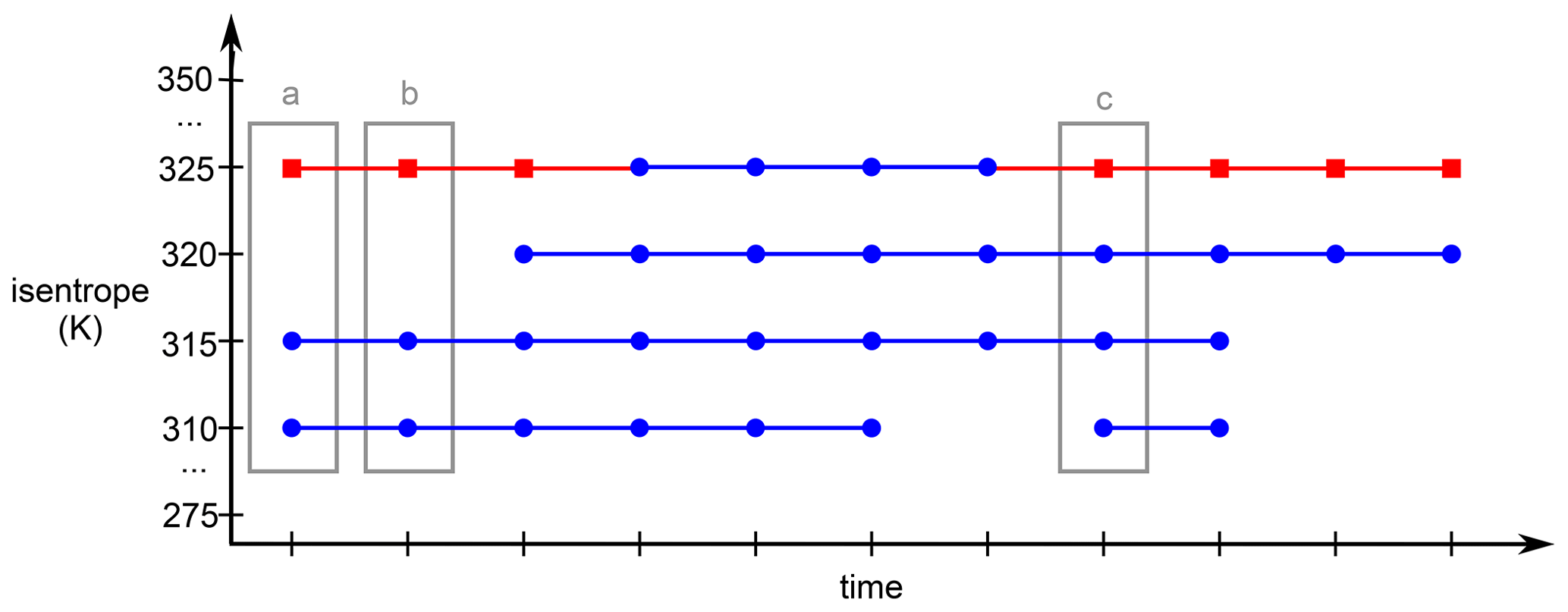
Figure 2 Schematic visualization of the construction of a 3D PV cutoff track from all overlapping isentropic 2D PV cutoff tracks. Isentropic 2D tracks making up the final 3D track are marked with blue lines and dots, and the isentropic tracks that are removed with red lines and squares. See text for a detailed discussion.

2.3.1 Tracking on isentropic surfaces

A 3D PV cutoff object consists of one or more 2D PV cutoffs, one on each isentropic level from 275–360 K. The 2D PV cutoffs at a given time t₀ are referred to as parents (gray features in Fig. 1). Isentropic tracks are constructed forward in time, by allowing only one successor per track (subsequently referred to as child, green features labeled accordingly in Fig. 1a–d); i.e., in the case of a splitting of a PV cutoff, the smaller part is ignored. This substantially eases the analysis of the tracks. From each parent, 6-hourly isentropic forward trajectories are started from each grid point (black crosses in Fig. 1), using the Lagrangian analysis tool Lagranto (Wernli and Davies, 1997; Sprenger and Wernli, 2015). A 2D PV cutoff at time t₀+6 h is a potential child if it inherits at least one air parcel from the considered parent. In the following, a variety of situations is considered that may occur during this step.

In the most simple situation, the movement of the 2D PV cutoff during this time interval is perfectly adiabatic (Fig. 1a), and all trajectories arrive within a 2D PV cutoff (the child) at the same level at time t₀+6 h (blue crosses in Fig. 1a). In a situation with diabatic activity (Fig. 1b), the adiabatic forecast of the PV cutoff (blue and red crosses in Fig. 1b) may deviate from reality at time t₀+6 h (the green feature in Fig. 1b). In this case, some trajectories end up outside of the child (red crosses in Fig. 1b), showing that the 2D PV cutoff shrinks due to STT. Also, the 2D PV cutoff may grow due to TST (orange cross in Fig. 1b). Note that here, STT is defined as the Lagrangian PV change of an air parcel from more to less than a value of 2 PVU, and vice versa for TST. If, additionally to STT and TST, splitting occurs (Fig. 1c), the 2D PV cutoff is selected as child that inherits most air parcels from the parent (lower green feature in Fig. 1c). The trajectories arriving within the other 2D PV cutoff(s) at time t₀+6 h (blue-gray crosses and upper green feature in Fig. 1c) are considered as shrinking due to splitting. It may also occur that two (or more) parents merge to one child (Fig. 1d). In this case, the child is attributed to the parent (parent 1 in Fig. 1d) from which it inherits more air parcels (number of blue crosses vs. number of gray crosses). The trajectories that the child inherits from the other parent(s) (parent 2 in Fig. 1d) are counted as growth due to merging and the track ends for the other parent(s). If the track of a 2D PV cutoff does not end via merging to another 2D PV cutoff, it either ends due to complete diabatic decay (Fig. 1e) or (complete or partial) reabsorption to the stratospheric reservoir (Fig. 1f). If all trajectories from the parent arrive in a region with PV < 2 PVU (red crosses in Fig. 1e), complete diabatic decay (involving STT) occurs. Air parcels arriving in a region with PV > 2 PVU but not within a PV cutoff are counted as reabsorption (blue crosses in Fig. 1f). In the case of merging, air parcels from the parent(s) for which the track ends (parent 2 in Fig. 1d) and that end up in the child are also considered as reabsorption. The two possibilities, reabsorption by the stratospheric reservoir and reabsorption by a larger cutoff, have relative frequencies of 89 % and 11 %, respectively.

Once all parents at time t₀ have been considered, the same is repeated for the subsequent time interval. In this way, tracks are continued for all 2D PV cutoffs identified as child in the previous time step, and new tracks are initialized for all other 2D PV cutoffs.

2.3.2 Construction of 3D tracks

After isentropic tracks are constructed, PV cutoff objects are concatenated to tracks representing the three-dimensional evolution. The resulting 3D tracks consist of at least one isentropic track but can include a large number of isentropic tracks on different isentropic levels. Because we aim to avoid branching of tracks, a major challenge in this step is to reasonably handle situations during which two or several isentropic tracks of a single 3D track do not contain the same PV cutoff object at a given time instant. This can occur as a result of merging and splitting. Consider, for example, the splitting situation illustrated in Fig. 1c. For the isentropic level shown, the isentropic track continues from the parent to the child and the lost child is dismissed. If, for example, such a splitting occurs simultaneously at another isentropic level where the PV cutoff labeled as “lost child” inherits more trajectories from the parent than the cutoff labeled as “child”, the two isentropic tracks are continued with a different PV cutoff object. Such a disagreement between tracks on different isentropic levels due to splitting is illustrated in Fig. 2 (see gray box with label c), where the track on 325 K is continued with a different PV cutoff object (red square) than on 310–320 K (blue dots). To create the non-branching 3D track, the following steps are required:

• i.

  Identify overlapping tracks. An isentropic track is selected, and all isentropic tracks on all isentropes are identified that at least once overlap with the selected track (i.e., contain the same 3D PV cutoff object). This search is repeated for all overlapping tracks until no further tracks are found (see all lines independent of the color in Fig. 2).

• ii.

  Create non-branching 3D track from overlapping tracks. The overlapping tracks are used to connect PV cutoff objects to a non-branching track according to the following rules: (a) the first time step, at which a track of the overlapping tracks exists at any isentropic level, marks the start of the 3D track. If there is more than one PV cutoff object at this time step that belongs to the overlapping tracks (which occurs if two tracks merge at a later time step), the dominant PV cutoff object is identified as the one with more isentropic levels or, if the number of levels is equal, the larger cutoff is selected (blue markers in the box (a) in Fig. 2). (b) Then, for the next time step, only PV cutoff objects are considered as successors if they are connected via an isentropic track with the previous PV cutoff object (blue markers in the box (b) in Fig. 2). (c) If rule (b) has been applied and still more than one PV cutoff object is part of the overlapping tracks at a later time step (which occurs if isentropic tracks are continued differently on different isentropic levels), the same criteria (depth and size) are applied as in rule (a) to select the dominant cutoff (blue markers in the box (c) in Fig. 2). Eventually, tracks are only retained if they have a minimum lifetime of 24 h.

A total number of 152 615 PV cutoff tracks provide the basis for this study, which is the largest dataset of PV cutoffs/COLs analyzed so far. On average, this amounts to over 300 PV cutoffs per month. To visualize tracks and locate genesis and lysis events the PV cutoff center is computed as the average of the coordinates of all grid points within the PV cutoff object weighted by their PV value. The area of the PV cutoff is determined as the area of the projection of the 3D PV cutoff onto a 2D plane; i.e., it includes all grid points that are part of the PV cutoff on at least one isentropic level. Examples demonstrating the application of the tracking to individual cases are shown in Sect. S3.

2.3.3 Limitations

The tracking method has two important limitations which are briefly mentioned here. First, only non-branching tracks are allowed and the decision criteria used may not represent the most reasonable track continuation in some cases. However merging and splitting are comparably rare. Therefore, this limitation does not question the usefulness of the method and the quality of the results presented here. At the poles, where merging and splitting occur more frequently and the definition of PV cutoffs becomes less obvious, this limitation is strongest. Second, the tracking procedure requires the computation of a large number of trajectories and is therefore computationally expensive. This makes its application less straightforward to datasets much larger than ERA-Interim or to operational ensemble forecasts for quasi-real-time purposes.

2.4 Classification of PV cutoffs according to their position relative to the jet streams and the limited role of statistical significance testing

In order to investigate whether different life cycle characteristics depend on the relative position of PV cutoffs to the jet streams, PV cutoffs are classified into three types: Type I (equatorward of the jet stream), Type II (between two jet streams), and Type III (poleward of the jet stream). Jet streams are identified according to Koch et al. (2006) as regions where the vertically averaged wind speed between 100 and 400 hPa exceeds 30 m s⁻¹. The jet-relative position of each PV cutoff is then determined as follows. All jet streams are identified that are intersected by the meridian through the PV cutoff center at genesis time. If jet streams are found only poleward of the PV cutoff, it is classified as Type I (22.4 % of all cutoffs). If jet streams are found poleward and equatorward of the PV cutoff, it is classified as Type II (33.2 %), and if jet streams are found only equatorward of the PV cutoff, it is classified as Type III (39.4 %). Few PV cutoffs cannot be classified because jet streams are absent at the longitude of PV cutoff genesis (5 %). This is mostly the case in the Northern Hemisphere in summer.

To draw statistically robust conclusions about observed differences between the three cutoff types (see Sect. 3.3), statistical significance testing has to be applied. However, in our case (using the Wilcoxon rank-sum and Kolmogorov–Smirnov tests), the sample sizes are so large that basically all differences between composite means or empirical distributions turn out to be statistically significant, even if they are relatively small. Hence, we will focus on differences that are (a) sufficiently large and (b) can be reasonably explained with physical arguments.

2.5 Linking PV cutoffs and surface cyclones

To study the link between PV cutoffs and surface cyclones, all surface cyclones are identified that reach spatial proximity to a PV cutoff. Here, spatial proximity occurs if the distance between the center of a surface cyclone and a PV cutoff is less than 600 km. Note that both, PV cutoffs and surface cyclones, are required to have a minimum lifetime of one day in this study.

3 Global climatology of PV cutoff life cycles

This section discusses a range of climatological aspects of PV cutoffs using the full global dataset. A comprehensive discussion of occurrence, genesis, and lysis frequencies is followed by the first climatological analysis of diabatic decay and reabsorption. Finally, PV cutoffs are separated into three categories, based on their relative position to the jet streams. For these categories, synoptic composites of PV cutoff genesis and the empirical distributions of various life cycle characteristics are analyzed.

3.1 Climatological frequencies

First, a detailed global overview of PV cutoff occurrence and favored genesis and lysis regions is provided and related to the climatology of the zonal upper-level flow. Given that this study presents the most comprehensive climatology of PV cutoffs so far, such an in-depth discussion is justified.

3.1.1 Frequencies of PV cutoff occurrence

We start with considering seasonal mean PV cutoff frequencies for boreal winter (DJF), spring (MAM), summer (JJA), and autumn (SON), as shown in Fig. 3. These frequencies indicate the percentage of time steps when a 3D PV cutoff is located at a particular grid point, independent of the number of levels covered by the 3D PV cutoff. PV cutoff frequencies are higher in the Northern Hemisphere (annual mean hemispheric average of 5.8 %) than in the Southern Hemisphere (4.0 %) in all seasons except DJF, when frequencies are about 1.2 percentage points larger in the Southern Hemisphere. Figure 3 shows a seasonal cycle with hemispheric averages about 30 % larger in summer than in winter in the Northern Hemisphere and about 2 times larger in the Southern Hemisphere. The number of tracks exhibits a much weaker seasonal cycle (not shown), indicating that cutoffs in summer tend to be longer-lived.

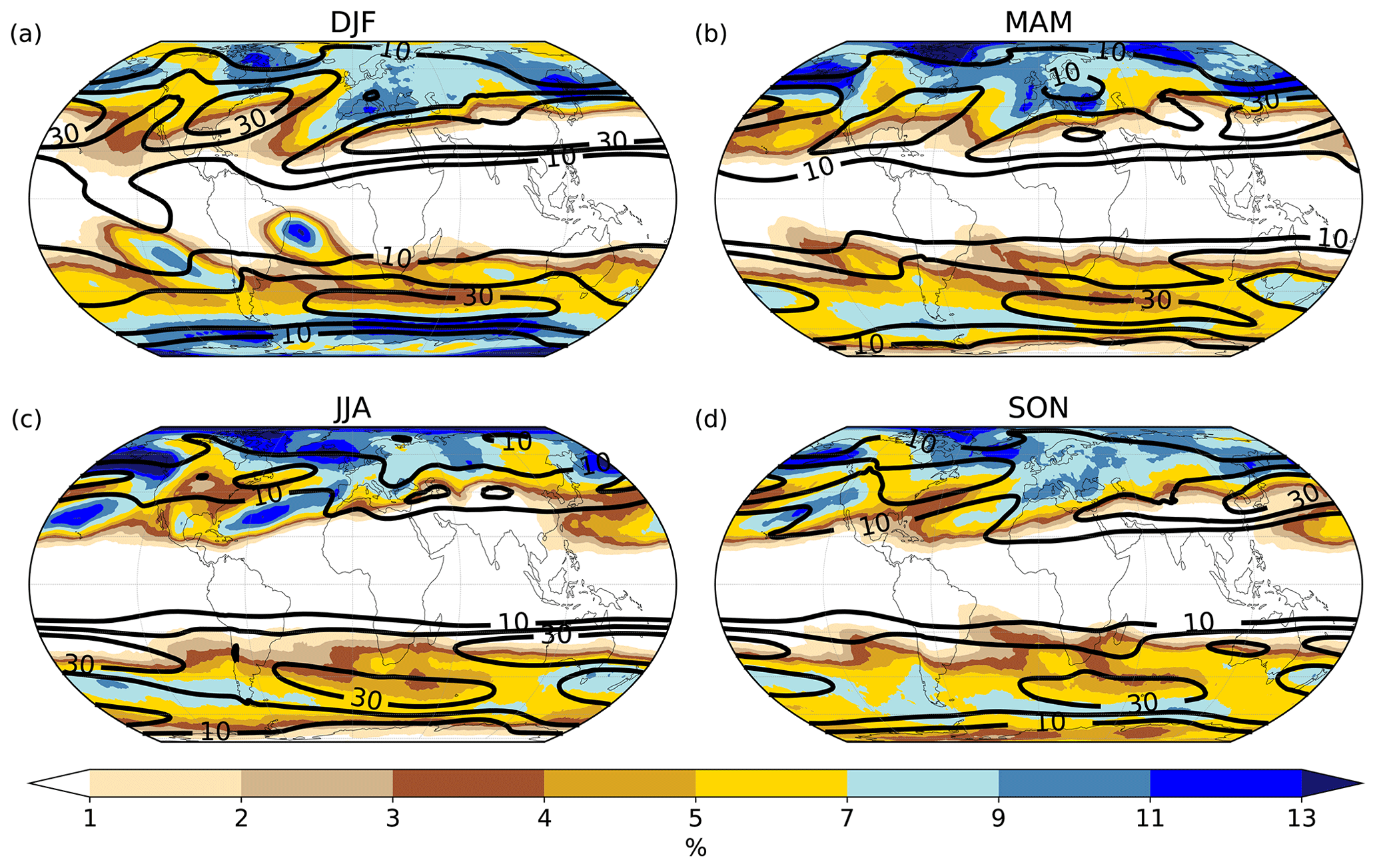
Figure 3 Seasonally averaged PV cutoff frequencies (shading, in %) and zonal wind speed (thick black line, 10, 20, and 30 m s⁻¹) for (a) DJF, (b) MAM, (c) JJA, and (d) SON.

In DJF (Fig. 3a), there is a large northern hemispheric maximum over southern Europe and the Mediterranean with frequencies up to 11 %. It coincides with the region of low upper-level zonal wind speeds (black lines in Fig. 3a) downstream of the North Atlantic storm track, where anticyclonic RWB occurs frequently (Martius et al., 2007; Bowley et al., 2019). Consistently, this frequency maximum is located poleward of the subtropical jet over northern Africa and equatorward of the North Atlantic jet stream. Note that, in Fig. 3, we identify the climatological positions of the jet streams based on maxima of the mean zonal wind speed. Similarly, the frequency maximum over the southwestern United States occurs in a region with frequent anticyclonic RWB downstream of the North Pacific storm track. Other frequency maxima in the Northern Hemisphere occur over northeastern Canada and the western North Atlantic, as well as the Russian Far East and the North Pacific. Some of these high frequencies coincide with maxima of cyclonic RWB in the storm track regions (Martius and Rivière, 2016; Bowley et al., 2019), but the high frequencies over the Canadian Arctic and the Russian Far East do not. However, they coincide with PV streamer maxima on 300 K (Wernli and Sprenger, 2007). This indicates that PV cutoffs in these regions may frequently result from PV streamers without significant cyclonic or anticyclonic tilt. A comparison to Hakim and Canavan (2005) also suggests a link to the occurrence of TPVs in these regions. In the Southern Hemisphere, PV cutoff frequencies have a clear maximum in a large tilted band from the central subtropical South Pacific towards the southeast reaching southern South America. A similar band is also present over the South Atlantic, with two maxima east of Brazil and west of South Africa. High frequencies occur also in the southern Indian Ocean and over New Zealand. These maxima are located equatorward of the jet stream and coincide with maxima of anticyclonic RWB (Song et al., 2011; Martius and Rivière, 2016). Further, PV cutoffs are frequent poleward of the jet stream along a circumpolar band at 60^∘ S around Antarctica, where cyclonic RWB is frequent (Song et al., 2011; Martius and Rivière, 2016).

In MAM (Fig. 3b), PV cutoff frequencies increase over the eastern parts of the North Atlantic and the North Pacific, as well as at high latitudes in the Northern Hemisphere. The frequencies in the Southern Hemisphere decrease in most regions, and the circumpolar band shifts equatorward and becomes less uniform. The subtropical jet stream appears over Australia, leading to split-jet conditions. A maximum appears over southern Australia, New Zealand, and the South Pacific between the polar and the subtropical jet streams. The summer maxima east of Brazil and in the subtropical South Pacific are absent in MAM.

In JJA (Fig. 3c), frequencies in the Northern Hemisphere further increase in the storm tracks (notably south of Iceland) and remain high at polar latitudes. The high frequencies in the storm track regions agree particularly well with the enhanced frequencies of cyclonic RWB there in JJA (Martius and Rivière, 2016). Further, as the North Atlantic and the North Pacific jet streams shift poleward and split-jet conditions over Europe and the United States disappear, PV cutoff frequencies in these regions strongly decrease compared to MAM. Instead, over the subtropical North Pacific and the subtropical North Atlantic large northeastward sloping bands of high frequencies appear. Similarly to their southern hemispheric counterparts in DJF, they are located equatorward of the jet stream in regions with frequent anticyclonic Rossby wave breaking (Martius and Rivière, 2016). The Southern Hemisphere is dominated by a zonal band between about 30 and 60^∘ N with local maxima over southern Australia and New Zealand, the central South Pacific, southern South America, and South Africa. These maxima coincide relatively well with maxima of anticyclonic Rossby wave breaking (Martius and Rivière, 2016).

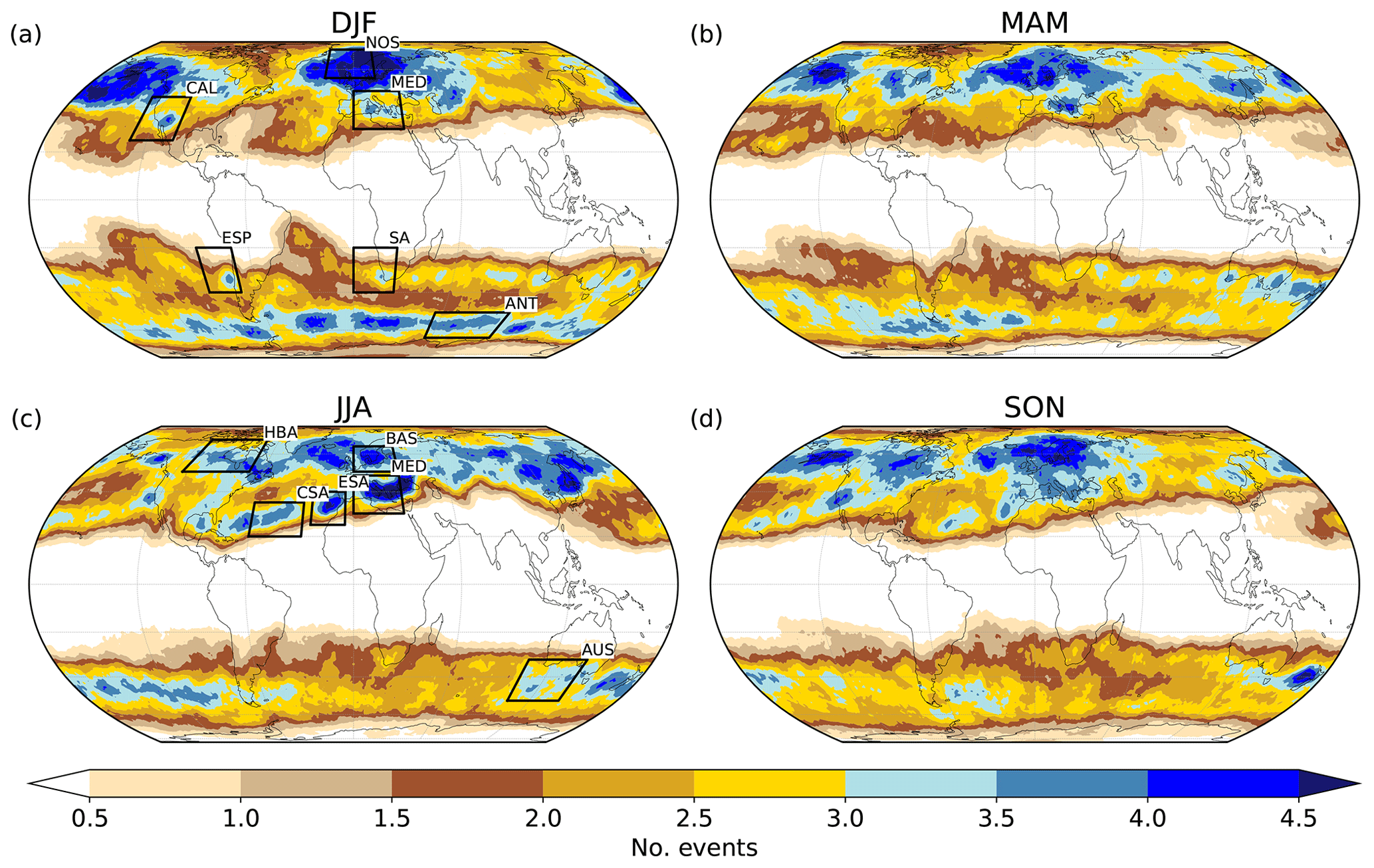
Figure 4 Seasonal average number of PV cutoff genesis events within a distance of 500 km in (a) DJF, (b) MAM, (c) JJA, and (d) SON. The location of a genesis event is determined by the center of the first PV cutoff of a track. Black boxes mark the genesis regions investigated in Sect. 4.

Frequencies in SON (Fig. 3d) are similar to MAM. Increasing frequencies compared to JJA are discernible over the United States, and central and southern Europe, as split-jet conditions start to re-establish. The maxima over the Arctic and in the North Pacific and the two bands in the subtropical North Pacific and North Atlantic are still visible, but frequencies substantially decrease compared to JJA. In the Southern Hemisphere, the circumpolar band shifts poleward and becomes more uniform again, and the tilted bands over the South Pacific and South Atlantic start to reappear.

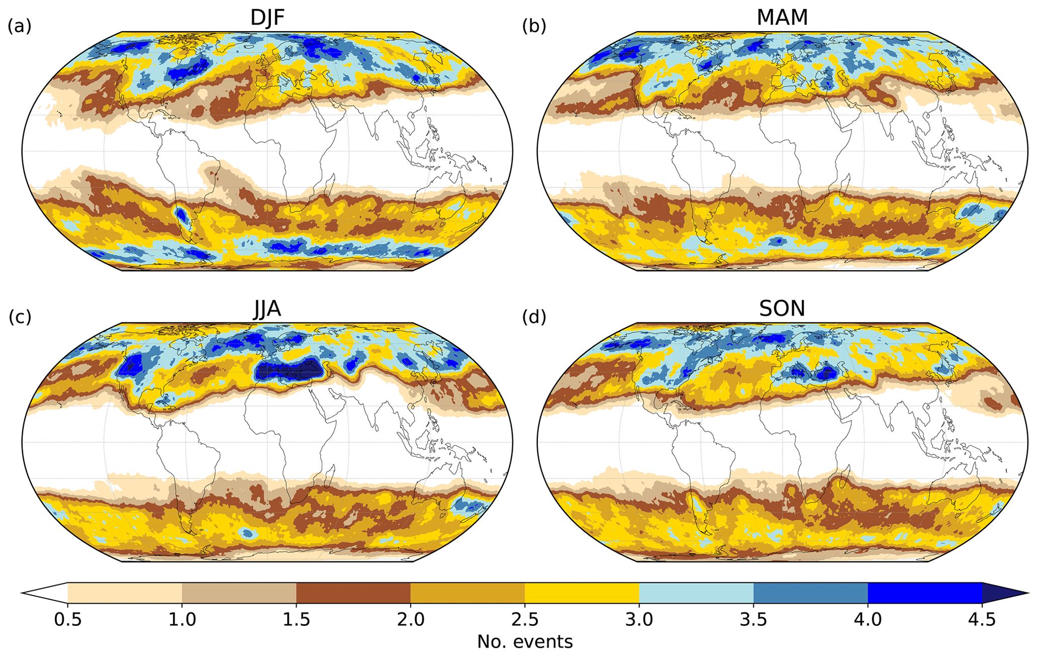
Figure 5 Seasonal average number of PV cutoff lysis events within a distance of 500 km in (a) DJF, (b) MAM, (c) JJA, and (d) SON. The location of a lysis event is determined by the center of the last PV cutoff of a track.

3.1.2 PV cutoff genesis and lysis frequencies

As a first step towards understanding the life cycles of PV cutoffs, it is insightful to look at the geographical locations of genesis and lysis. Note again that lysis can be due to reabsorption or diabatic decay. Figures 4 and 5 show seasonal maps of the number of genesis and lysis events per season that occur within a 500 km distance of each grid point. In some regions, maxima in genesis frequencies disagree with maxima in PV cutoff frequencies. For example, while genesis maxima also coincide with cutoff frequency maxima over California and the Mediterranean, genesis is particularly frequent in the eastern part of the storm tracks (Fig. 4a), but PV cutoff frequencies are larger in the western parts (Fig. 3a). In the Southern Hemisphere in DJF the well-known (see Sect. 1) genesis maxima close to the west coast of South America and west of South Africa are visible (Fig. 4a). As PV cutoff frequencies, PV cutoff genesis frequencies can largely be understood as the result of the climatological large-scale flow conditions and corresponding positions of the jet streams in the respective seasons (cf. Fig. 3 and associated discussions). For example, the genesis maxima in the storm tracks are located within or downstream of maxima of cyclonic RWB (Martius and Rivière, 2016; Bowley et al., 2019) further indicating that PV cutoffs in the storm tracks are mainly a consequence of cyclonic RWB. For PV cutoff lysis frequencies, additional aspects seem to be important. For example, some lysis maxima occur over land related to orography (e.g., in DJF and SON over South America and South Africa (Fig. 5a and d), in JJA over the Rocky Mountains/Pacific Coast Ranges and over the Iberian Peninsula (Fig. 5c), and in JJA and SON over Greece, Turkey, and the Balkans (Fig. 5c and d)), whereas others occur over sea surfaces, in particular where enhanced sea surface temperatures are expected (e.g., in all seasons over the Mediterranean, in JJA over the Caribbean, and in regions of all western boundary currents; e.g., in DJF over the western North Atlantic and in JJA east of Australia). A further conspicuous lysis maximum is discernible over the central United States/the southern Rocky Mountains in all seasons, which could be related to orography and/or the supply of moist and warm air from the Gulf of Mexico. These patterns suggest an important role of diabatic effects on PV cutoff lysis, e.g., due to friction and orography, land/sea surface–atmosphere interactions, and convection. However, lysis frequencies are also high in regions where diabatic effects are not expected to be particularly strong, e.g., in the Southern Ocean around Antarctica in all seasons or over Russia and Alaska in DJF.

3.1.3 Link to previous studies

A range of previous studies have addressed climatological frequencies of PV cutoffs. In the following, we relate our results to these studies and summarize the main new insight gained from the results presented here. Many of the presented frequency, genesis, and lysis maxima of PV cutoffs are consistent with previous climatological studies. In the Southern Hemisphere, most maxima agree well with the results of Fuenzalida et al. (2005), Reboita et al. (2010), and Pinheiro et al. (2017). In the Northern Hemisphere, they compare favorably with Nieto et al. (2005) mainly in subtropical latitudes, with, e.g., Bell and Bosart (1989) in higher latitudes, and with Munoz et al. (2020) in most regions if COLs at both 500 and 200 hPa are considered. However, in this study all of them are identified based on a consistent methodology and independent of the selection of a vertical level. This has also implications for the seasonality of PV cutoffs. Several previous studies found a clear seasonal cycle with about 4 times more COLs forming in summer than in winter in both hemispheres and that seasonality depends strongly on the considered pressure level (Nieto et al., 2005; Reboita et al., 2010; Munoz et al., 2020). The seasonal cycle in this study is much weaker, in agreement with the findings of Wernli and Sprenger (2007), if they took into account all isentropic levels from 305–370 K. Hence, it seems that the strong seasonal cycle found in previous studies is mainly related to the seasonal cycle of the vertical (pressure or isentropic) level on which PV cutoffs/COLs occur (for illustration of this aspect, see Wernli and Sprenger, 2007, their Fig. 8b).

Further, some of the identified maxima have not or have only been described little in the literature before. In particular, the circumpolar band around Antarctica and the far equatorward reaching band in the South Pacific in DJF have not been documented as regions of COL occurrence yet. The circumpolar band around Antarctica and its seasonal change in symmetry agrees very well with the climatology of upper tropospheric storm track features discussed in Hoskins and Hodges (2005). The maximum east of Brazil was mentioned only by Reboita et al. (2010) and Crespo et al. (2021).

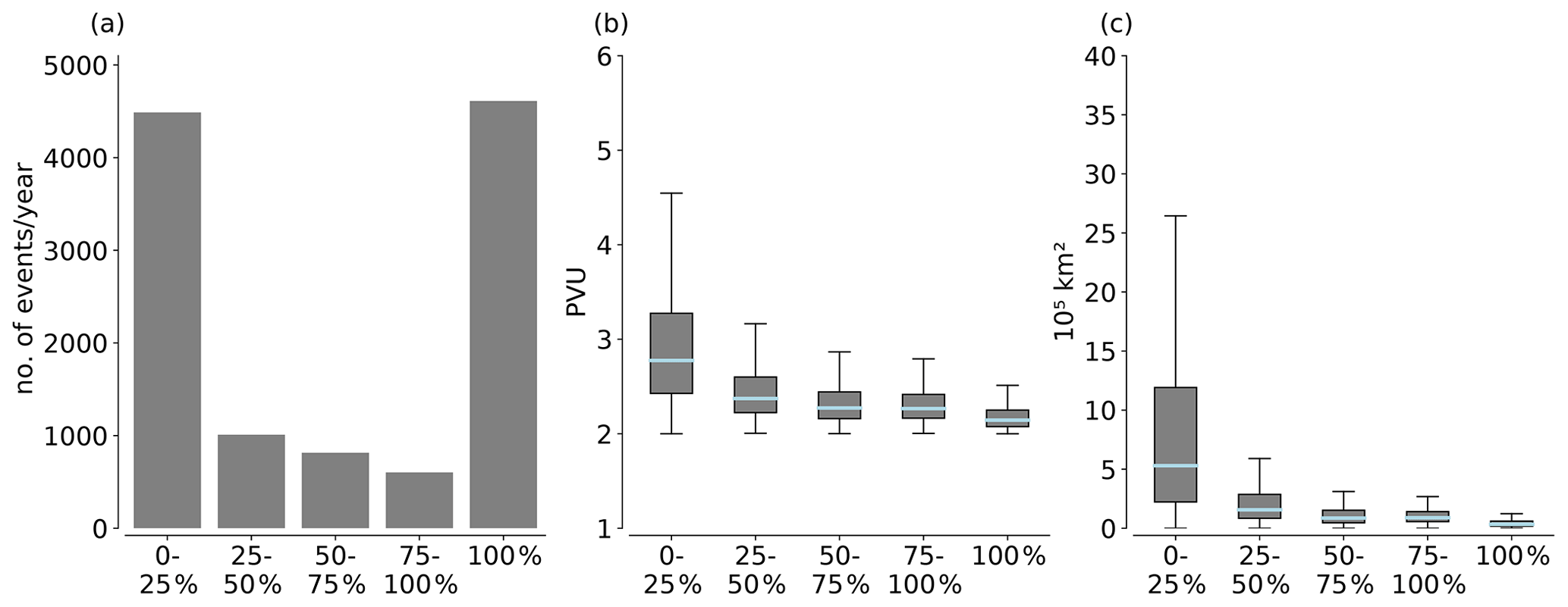
Figure 6 (a) Histogram of the percentage of air parcels in a PV cutoff experiencing decay whenever the PV cutoffs disappear on an individual isentrope (average annual number of events, 0 % corresponds to pure reabsorption, 100 % to complete diabatic decay), and (b, c) standard box plots (outliers not shown) of (b) mean PV and (c) area of the PV cutoff at the isentropic level from which it disappears for the histogram classes in (a).

Finally, our global analysis reveals also general global patterns of PV cutoff occurrence and its relation to other elements of the atmospheric circulation. PV cutoffs in summer occur frequently in the subtropics mostly in east- and poleward tilted bands reaching latitudes around 20^∘ over the Pacific and Atlantic equatorward of the jet stream, and another one at higher latitudes, in particular in the storm track regions poleward of the jet stream. In winter, PV cutoffs occur either poleward of the jet stream or, particularly frequently, in regions with split-jet conditions between the polar and subtropical jet streams. A comparison to the climatology of jet streams (Koch et al., 2006) further supports these relationships between jet streams and PV cutoffs. It shows that high PV cutoff frequencies often occur slightly poleward of jet frequency maxima (western North Atlantic, Japan, around Antarctica in DJF), poleward of the subtropical jet maxima and equatorward of the polar jet maxima (Mediterranean and central Europe in DJF, Australia in JJA), or in regions where strong jet streams are absent, in particular over the subtropical ocean basins in summer. This link to jet streams will be used for a classification of PV cutoffs in Sect. 3.3. Further, some PV cutoff frequency maxima are in striking agreement with high cyclone frequencies. For example, the frequency maxima over the Canadian Arctic and south of Iceland in JJA agree particularly well with the surface cyclone maxima found by Wernli and Schwierz (2006). Frequency maxima over the southern Indian Ocean close to Antarctica in DJF also correspond well with surface cyclone maxima identified by Jones and Simmonds (1993). Together with the discussed agreement with frequencies of cyclonic RWB, this suggests that, in particular regions, PV cutoff life cycles are strongly linked to the baroclinic life cycles of extratropical cyclones. This aspect will be further investigated in Sect. 3.3 for cutoff categories and in Sect. 4.4 for selected geographical regions.

3.2 Quantification of diabatic decay and reabsorption

In the following, we address an aspect of PV cutoff life cycles that, so far, has not been investigated climatologically: do they disappear on an isentrope due to diabatic decay or reabsorption to the stratospheric reservoir? According to Hoskins et al. (1985) and based on “synoptic experience”, diabatic decay is the dominant scenario. Here, we provide the first quantitative answer to this long-standing question in dynamical meteorology. This quantification will be useful to better understand global climatological patterns of PV cutoff lysis, the modification of PV cutoffs by diabatic processes, as well as their vertical evolution.

Whenever a PV cutoff disappears on an isentropic surface, we quantify what fraction of the PV cutoff experiences diabatic decay (i.e., undergoes STT) and what fraction is reabsorbed by the stratospheric reservoir (see Sect. 2.3 and Fig. 1e and f). The diabatic decay fraction of a single cutoff can vary between 0 % (pure reabsorption) and 100 % (complete diabatic decay). Intermediate values indicate simultaneous partial reabsorption and partial decay. Note that this analysis identifies events on isentropic surfaces, which means that, even if a 2D PV cutoff disappears, the 3D PV cutoff may still persist afterwards. Therefore, reabsorption and decay can, in principle, occur during the entire PV cutoff life cycle. Here, we first investigate the overall statistics of decay and reabsorption and then provide a global overview of the geographical distribution of these two possible scenarios.

Figure 7 Average number of (a, c) reabsorption (less than 50 % decay, blue shading) and (b, d) diabatic decay (more than 50 % decay, red shading) events per season within a distance of 500 km for (a, b) DJF and (c, d) JJA. As a reference, the contour for five reabsorption events per season (blue contour) is shown (b, d).

Figure 6a shows the decay and reabsorption statistics for five different categories of the decay fraction for all 2D PV cutoffs identified globally. It shows that almost pure reabsorption (decay fraction < 25 %) is equally frequent as complete diabatic decay (decay fraction = 100 %), while intermediate scenarios are relatively rare. Considering all events with a decay fraction of <50 % as reabsorption and all other events as diabatic decay shows that reabsorption accounts for almost half (47 %) of the disappearances of 2D PV cutoffs. During lysis of 3D PV cutoffs, i.e., if only the last time step of each PV cutoff life cycle is considered, reabsorption is, with a share of 54 %, even a little more frequent than diabatic decay. This result disagrees with the expectation by Hoskins et al. (1985) that diabatic decay dominates. Figure 6b and c provide the following explanation for this result: reabsorption predominantly occurs for large PV cutoffs with comparatively high PV values. For an individual 3D PV cutoff this is usually the case on higher isentropic levels, where it is closer to the stratospheric reservoir. Hence, at higher levels, chances are high that the PV cutoff is reabsorbed by the stratospheric reservoir. It may also occur that the reabsorption is transient; i.e., a PV cutoff is reabsorbed and later again detached from the stratospheric reservoir several times during its life cycle. This behavior has been shown by Portmann et al. (2018) for two case studies over Europe. Complete diabatic decay, on the other hand, occurs typically at lower levels where the PV cutoff is smaller and has lower PV values. We conclude that, on a global average, diabatic decay and reabsorption are equally relevant for the three-dimensional life cycles of PV cutoffs.

The geographical distributions of reabsorption and diabatic decay events of 2D PV cutoffs are visualized in Fig. 7. The maps show the seasonal mean frequency of reabsorption (Fig. 7a and c) and decay (Fig. 7b and d) occurrence within a 500 km distance of a particular grid point in DJF and JJA. The geographical patterns of both categories resemble the PV cutoff frequencies presented in Fig. 3, revealing that they can both occur during all phases of the life cycle of the 3D cutoff. However, frequencies are particularly high where also lysis frequencies are high (Fig. 5a and c). Lysis maxima at higher latitudes are preferentially near reabsorption maxima and at lower latitudes near decay maxima. During DJF, in particular the lysis maxima over the central/southern United States, the US east coast, the Mediterranean, southern South America, South Africa, and southeast of Australia are dominated by diabatic decay and the ones over Alaska, Russia, and the Southern Ocean around Antarctica by reabsorption. In JJA, diabatic decay dominates lysis maxima over the western United States, the Mediterranean, the Caribbean, South Africa, and south of Australia. Reabsorption more strongly contributes to lysis maxima over the northern North Pacific, the Hudson Bay, south of Iceland, and again the Southern Ocean around Antarctica. Hence, even if they are roughly equal on a global average, the frequencies of diabatic decay and reabsorption strongly depend on the region.

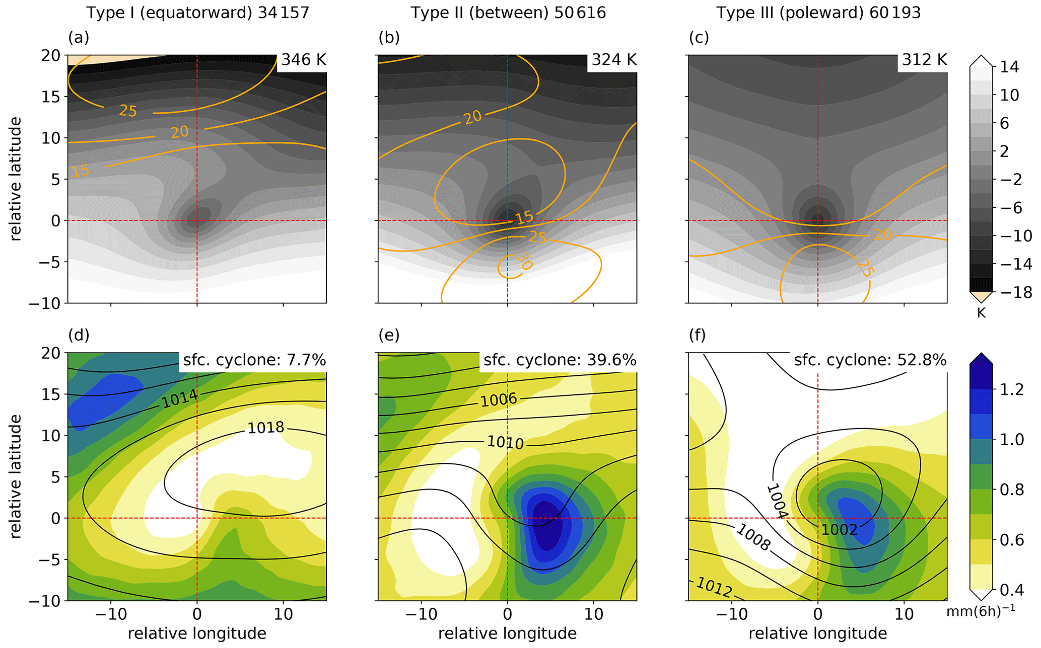
Figure 8 Cutoff-centered composites of (a–c) equivalent potential temperature at the 2 PVU isosurface (shading, in K, given as difference from the domain mean value indicated at the top right of each panel) and zonal wind speed at 300 hPa (orange contours, in m s⁻¹), and (d–e) total precipitation (shading, in mm (6 h)⁻¹) and sea level pressure (black contours, in hPa) at PV cutoff genesis, individually for (a, d) Type I, (b, e) Type II, and (c, f) Type III. The total number of tracks of each type is indicated at the top of panels (a)–(c). Additionally, the percentage of PV cutoffs linked to a surface cyclone during their life cycle is indicated for each type at the top right of panels (d)–(f).

3.3 Climatological characteristics of PV cutoffs with different positions relative to the jet streams

The discussion of climatological frequencies in Sect. 3.1 suggested a strong relationship between PV cutoff occurrence and the position of jet streams. Additionally, Sect. 3.2 showed that a central characteristic of PV cutoff life cycles, the frequencies of decay and reabsorption, has a remarkable regional variability. In this section, we investigate characteristics of the life cycles of PV cutoffs, which differ in terms of their position relative to the jet streams. This not only provides insight into fundamental properties of PV cutoff life cycles, but also serves to explain parts of their regional variability. To this end, PV cutoffs are classified into three types: Type I forms equatorward of the jet stream, Type II between the polar and the subtropical jet streams, and Type III poleward of the jet stream (for details see Sect. 2.4). This classification of PV cutoffs according to the jet-relative position follows early studies by Bell and Bosart (1989) and Price and Vaughan (1992). According to the considerations in Sect. 3.1 and the fundamental understanding of RWB and baroclinic life cycles (e.g., Thorncroft et al., 1993; Wernli et al., 1998), the jet-relative position is expected to be strongly linked to the type of wave breaking resulting in PV cutoff formation. Therefore, the classification used here is also related to the one proposed by Palmén and Newton (1969), which was based on the shape of the breaking upper-level wave. Please note that the Sect. S3 (Figs. S2–S4) illustrates example cases for each of the three types.

The climatological frequencies of the three types reveal that each occurs in preferred regions with different seasonal cycles (see Sect. S1, Fig. S1 in the Supplement). The summer maximum in the subtropical ocean basins is dominated by Type I cutoffs. In the other seasons, in particular winter and spring, this cutoff type is infrequent. On the contrary, Type II occurs most frequently in winter in mid-latitudes between about 30–50^∘ latitude and particularly frequently in regions with split-jet conditions (e.g., the Mediterranean, California, Australia, New Zealand). Type II hardly occurs in summer and has moderate frequencies in the autumn and spring. Finally, Type III occurs at higher latitudes and in the storm track regions all year around.

The regional differences in their occurrence already suggest that the meteorological environment may strongly vary between the three types. In the following, synoptic composites at the time of PV cutoff genesis are presented for each of the three types. The composites contain all PV cutoffs of the respective type in the dataset, i.e., cutoffs in all seasons and both hemispheres (fields from the Southern Hemisphere are flipped in the meridional direction). The environment of Type I is characterized by a strongly anticyclonic tilt of the potential temperature field at the dynamical tropopause, which is a clear sign of anticyclonic Rossby wave breaking (Fig. 8a). The wave breaking occurs in a region with anticyclonic wind shear equatorward of the jet stream, as indicated by the composite zonal wind (Fig. 8a). Type I PV cutoffs form over a surface anticyclone and result in only weak surface precipitation (Fig. 8d). Type II PV cutoffs are also the result of anticyclonic RWB equatorward of the jet stream, albeit with a weaker anticyclonic tilt (Fig. 8b). Consistently and in contrast to Type I, the wind speed increases also equatorward of the PV cutoff, resulting in a cyclonic barotropic shear and counteracting the anticyclonic tilting of the PV streamer. Such a situation can result in a cyclonic break-up of the tip of the PV streamer (as for the case shown in Fig. S3), featuring a mixture between anticyclonic and cyclonic RWB (Berrisford et al., 2007). Type II has the highest precipitation rates among the three types (Fig. 8e). Precipitation is highest east of the cutoff center, where the sea level pressure field shows signatures of a developing surface cyclone. Finally, Type III cutoffs form from an upper-level wave with no or a slight cyclonic tilt poleward of the jet stream (Fig. 8c). They are associated with a pronounced surface cyclone and substantial precipitation (Fig. 8f, although less than for Type II).

To gain insight into the quantitative link between PV cutoffs and surface cyclones beyond composites, the two weather systems are linked on an event basis. It is well established that upper-level PV anomalies can play an important role for the genesis and intensification of surface cyclones (e.g., Hoskins et al., 1985; Reader and Moore, 1995; Wang and Rogers, 2001; Campa and Wernli, 2012; Graf et al., 2017) and thereby strongly affect surface weather. As noted in the introduction, PV cutoffs have been linked to surface cyclones for individual cases or climatologically within certain regions. While most studies focused on surface cyclones and then considered potentially associated upper-level PV anomalies, here, we focus on PV cutoffs and ask how often we find surface cyclones in their proximity (for methodological details see Sect. 2.5). Consistent with the composite sea level pressure, the frequency with which a PV cutoff is close to a surface cyclone during its life cycle varies substantially among the three types (see percentages in Fig. 8d–f). More than half of Type III cutoffs, almost 40 % of Type II cutoffs, and less than 8 % of Type I cutoffs are linked to surface cyclones. It is also interesting to note that even for Type III, a substantial fraction of PV cutoffs is never linked to a surface cyclone.

These results reveal that there are fundamental meteorological differences between the three PV cutoff types, supporting the view point that the formation of PV cutoffs with different jet-relative positions can be understood as a result of the two archetypal baroclinic wave life cycles (LC1 and LC2, Thorncroft et al., 1993). LC2 results in cyclonic RWB and PV cutoffs poleward of the jet stream, often close to the surface cyclone (Type III). LC1 results in anticyclonic RWB and PV cutoffs equatorward of the jet stream in summer (Type I) and between the polar and the subtropical jet streams in winter (Type II). These PV cutoffs are well separated from the primary surface cyclone (which generally remains confined to the storm track regions). However, the formation of Type II cutoffs can be related to secondary cyclogenesis downstream of the primary surface cyclone. From an impact point of view, Type II cutoffs are of particular interest. They are not only associated with the highest precipitation rates and a significant influence on the surface pressure field, but also frequently occur in populated areas.

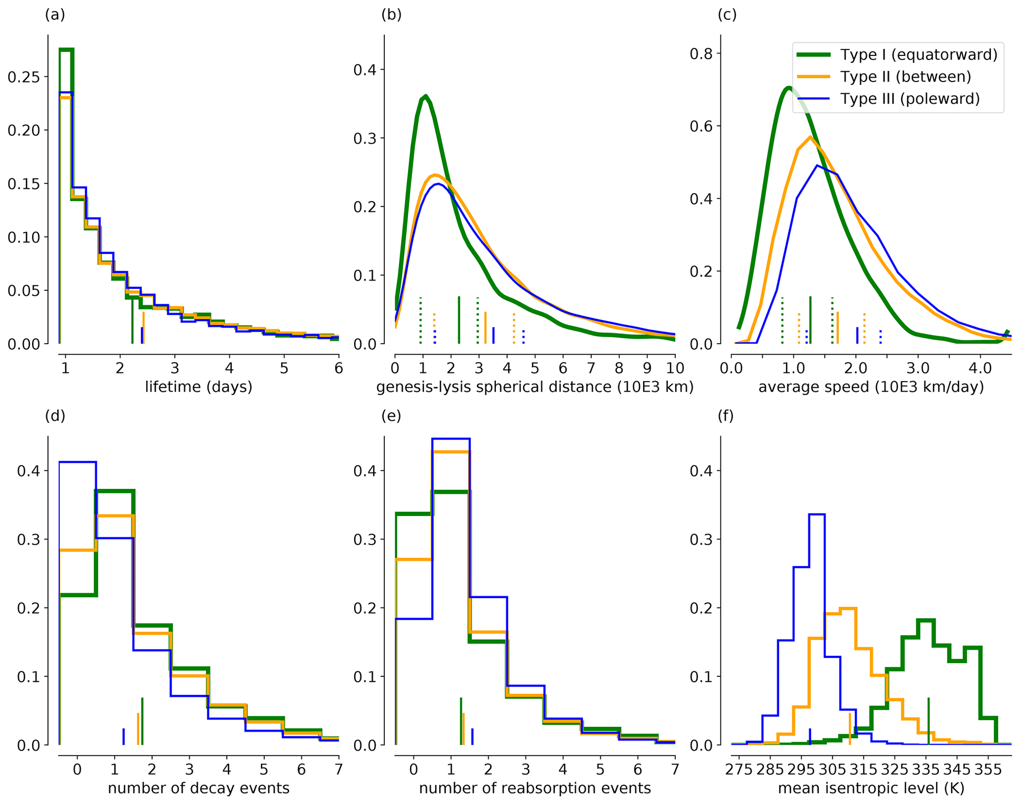
Figure 9 Empirical distributions of (a) lifetime, (b) spherical distance between genesis and lysis locations, (c) average propagation speed, (d) number of decay events, (e) number of reabsorption events, and (f) the mean isentropic level during the life cycle PV cutoffs of Types I, II, and III. (a, d, e, f) Distributions are shown as normalized histograms with the bar widths corresponding to unity; i.e., the vertical axis values can be read as percentages. (b, c) Distributions are shown as density estimates. Vertical lines indicate (solid) mean values and (dashed) upper and lower quartiles.

Next, some basic characteristics of the life cycle of the three PV cutoff types are analyzed and compared. To this end, empirical distributions of six characteristics are shown for each type in Fig. 9. For continuous variables we show density distributions and for discrete variables normalized histograms. The lifetime shows a roughly exponential decay after the minimum duration of one day required in this study. The distributions are very similar for the three cutoff types, with a tendency for Type I (equatorward of jet) to last shorter than the others (Fig. 9a). Larger differences appear for the spherical distance between genesis and lysis, which is substantially smaller for Type I cutoffs (Fig. 9b). The mean is slightly above 2000 km, while it is about 50 % larger for Types II (between jets) and III (poleward of jet). Consistently, the average propagation speed is also lowest for Type I, followed by Type II and Type III. These differences are of course related to the preferred regional occurrence of the three types. While Type I occurs preferentially in regions with low climatological zonal wind speed, Type III occurs in the storm tracks, where zonal winds are stronger. Type II occurs in regions with moderate zonal wind speed, and consequently its propagation speed is intermediate. These results also show that the picture that PV cutoffs are mainly quasi-stationary systems is misleading. In fact, many PV cutoffs travel several thousand kilometers. This result stands in contrast to studies pointing out the quasi-stationarity of COLs (e.g., Bell and Bosart, 1989; Pinheiro et al., 2017) or even assume it to justify assumptions for the tracking procedure (e.g., Munoz et al., 2020). The frequent occurrence of PV cutoffs with lifetimes between 1–2 d is in agreement with earlier studies (e.g., Kentarchos and Davies, 1998; Nieto et al., 2005; Reboita et al., 2010), except from Pinheiro et al. (2017), who found average lifetimes of 6–8 d. Differences in mobility and lifetime most likely arise from the different identification and tracking methods.

Two other key characteristics of PV cutoff life cycles are the frequencies of decay and reabsorption. Section 3.2 already pointed out that substantial regional differences exist. Here, we find that for Type III cutoffs reabsorption is more frequent and, consistently, decay less frequent than for the two other types (Fig. 9d and e). More than 80 % of all Type III PV cutoffs experience at least one reabsorption event, but only slightly less than 60 % experience a decay event. For Type I, these numbers are 65 % for reabsorption and 80 % for decay. Also here, Type II has intermediate values. A reason for these differences could be that Type I and Type II cutoffs are generally further away from the stratospheric reservoir, rendering reabsorption less probable.

Finally, the mean isentropic level of the PV cutoff during its life cycle is considered (Fig. 9f). Consistent with earlier studies and the composite analyses (Fig. 8a–c), the differences between the three types are substantial. Type I occurs mainly above 325 K, Type II between 300 and 320 K, and Type III between 290 and 305 K. In addition, the distribution is narrower for Type III compared to the other two types. These results further demonstrate the importance of considering a large range of isentropic levels to capture all PV cutoffs in different regions and seasons.

4 PV cutoff life cycles in selected genesis regions

In the first part of this article, global patterns and characteristics of PV cutoff life cycles were discussed and it was shown that the position relative to the jet streams helps to explain some of the large variability of PV cutoff life cycles. Previous case studies (e.g., Gouget et al., 2000; Garreaud and Fuenzalida, 2007; Singleton and Reason, 2007a; Portmann et al., 2018; Mohr et al., 2020) suggested that the life cycles of PV cutoffs including their surface impacts can also be strongly modified by characteristics of a specific geographical region (e.g., orography, moisture availability, and sea surface temperatures). In addition, there is a particular interest in the scientific community to study PV cutoffs and their impacts in specific geographical regions systematically, for example in Europe and the Mediterranean (e.g., Porcu et al., 2007), North America (e.g., Abatzoglou, 2016), East Asia (e.g., Hu et al., 2010), South America (e.g., Campetella and Possia, 2007), South Africa (e.g., Favre et al., 2013), and Australia (e.g., Singleton and Reason, 2007b). Therefore, in this section, subsets of PV cutoff tracks are investigated, selected according to their genesis within clearly defined geographical regions. This approach is complementary to the separation of PV cutoffs according to their jet-relative position. We demonstrate here that the global climatology is useful to perform regional analyses of PV cutoffs based on a consistent methodology, allowing for a better quantitative comparison of PV cutoff life cycles across geographical regions than was previously possible.

In DJF and JJA, six genesis regions are selected subjectively, also considering regions that were previously discussed in the literature (see black boxes in Fig. 4a and c; for more details see Table S1 in the Supplement). This selection does by no means include all interesting regions (it contains roughly 6 % of cutoff tracks in the dataset), and we encourage the community to use our dataset for further analyses. In the following, various aspects of the life cycles of PV cutoffs with genesis in these 12 regions are investigated. We start with a discussion of PV cutoff tracks and then discuss their vertical evolution and lifetimes. The vertical evolution is then linked to the occurrence of diabatic decay and reabsorption along the life cycles. Finally, the last part of this section investigates the link to surface cyclones, in particular focusing on the chronology of the life cycles of PV cutoffs and surface cyclones.

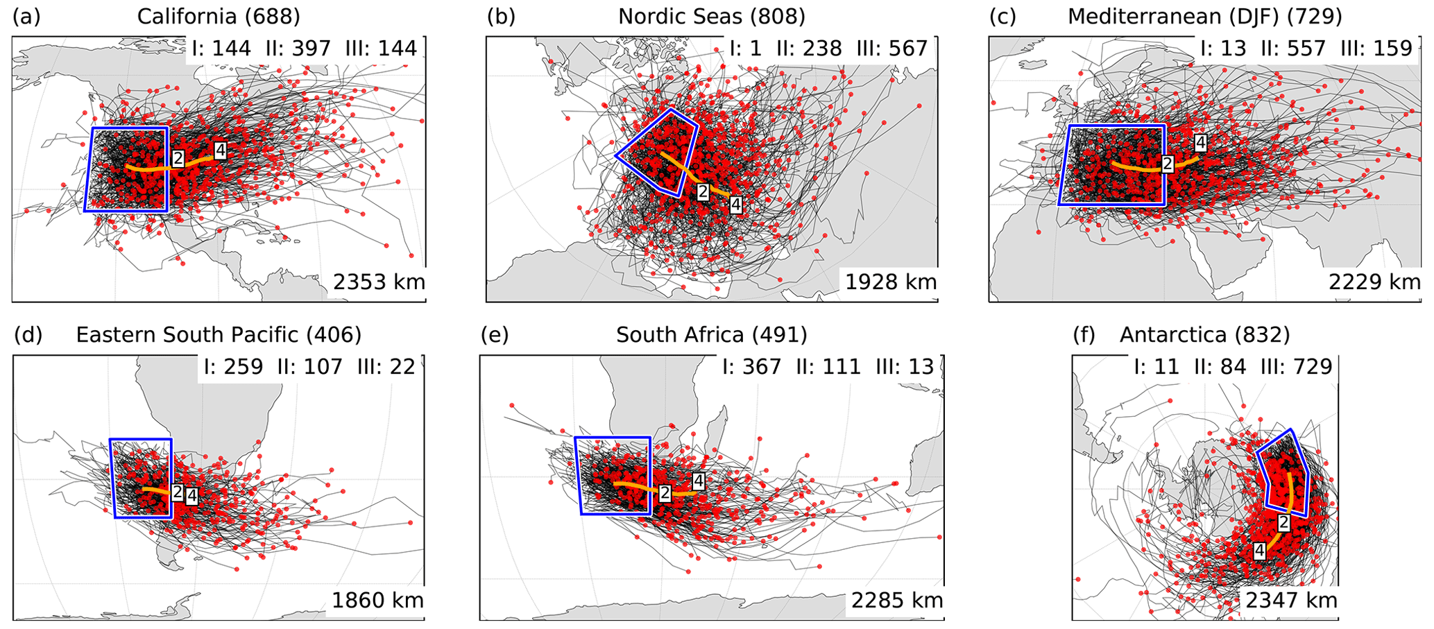
Figure 10 All tracks (black lines), lysis points (red dots), and average tracks (orange lines, including average location at days 2 and 4) of PV cutoffs with genesis over the six selected regions (blue boxes) in DJF: (a) California, (b) Nordic Seas, (c) Mediterranean, (d) eastern South Pacific, (e) South Africa, and (f) Antarctica. The average spherical distance between genesis and lysis is indicated at the bottom right of each panel.

4.1 PV cutoff tracks

First, an overview of the tracks is presented for all selected genesis regions. Figure 10 shows the tracks and lysis points for the six regions selected in DJF. In all regions, PV cutoffs tend to travel eastward. Most PV cutoffs forming over California move across the Rocky Mountains, where some tracks already end (Fig. 10a), consistent with the lysis maximum there in Fig. 5a. However, many continue to move northeastward over the southern and eastern United States, and some even travel far into the North Atlantic. PV cutoffs forming over the Nordic Seas often remain in this area or move towards northern Europe, but some even propagate into the Mediterranean, towards the North Pole, or across Russia (Fig. 10b). PV cutoffs with genesis over the western Mediterranean first travel southeastward across the Mediterranean and then tend to move on a more eastward or northeastward path over eastern Europe and the Middle East, where many tracks end (Fig. 10c). The tracks with genesis over the eastern South Pacific and over South Africa are strikingly similar (Fig. 10d and e): they lead southeastward across the southern tips of South America and South Africa, where many tracks end over land, and some cutoffs travel further into the South Atlantic and the South Pacific, respectively. However, PV cutoffs over South Africa travel on average about 400 km farther. PV cutoffs forming close to Antarctica travel relatively zonally eastward and a few almost fully around Antarctica (Fig. 10f). In each of the regions one particular PV cutoff type dominates but to differing extents. For example, over the Nordic Seas and the Antarctic Ocean, Type III (poleward of jet) is most frequent. However, while it strongly dominates over the Antarctic Ocean (almost 90 % of the cases), Type II (between jets) is also frequent over the Nordic Seas (only 70 % of Type III). The average spherical distance between genesis and lysis ranges between 1860 and 2353 km and is therefore well within the interquartile range of all types shown in Fig. 9b.

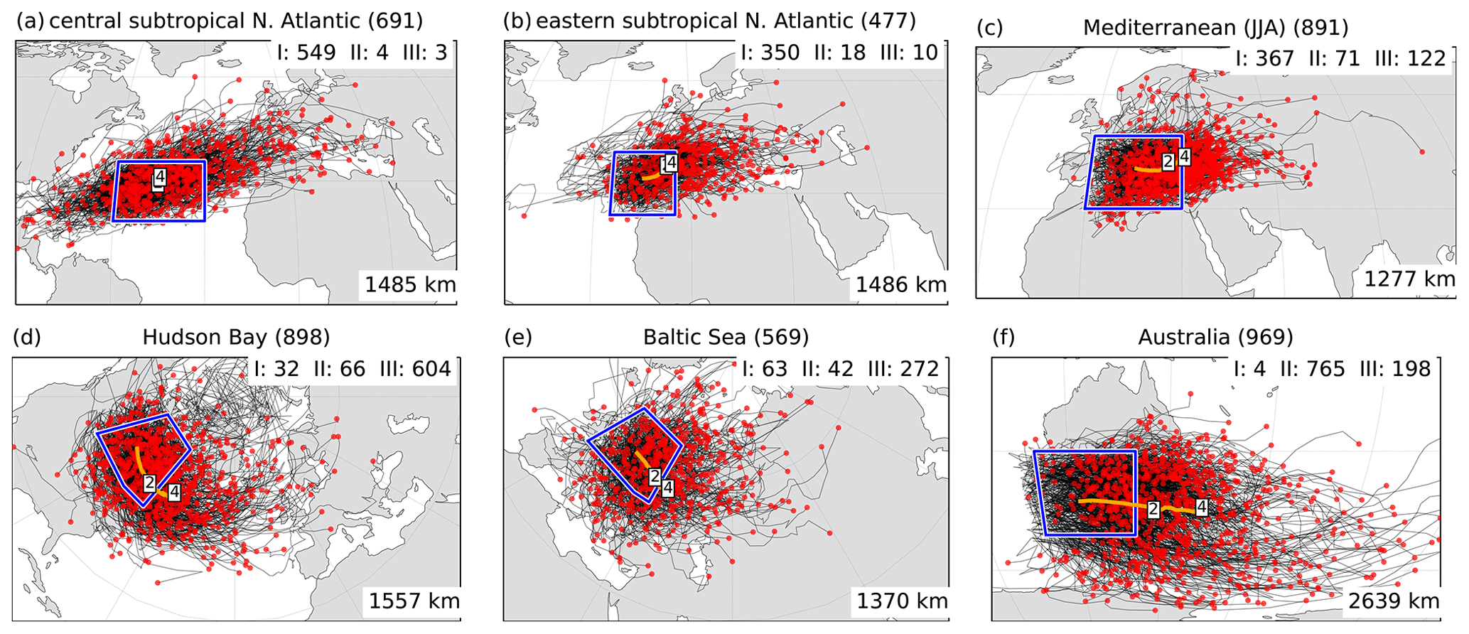
Figure 11 Same as Fig. 10 but for JJA and (a) central subtropical North Atlantic, (b) eastern subtropical North Atlantic, (c) Mediterranean, (d) Hudson Bay, (e) Baltic Sea, and (f) Australia.

In JJA (Fig. 11), PV cutoffs also travel eastward on average in all selected regions except the ones forming over the central subtropical North Atlantic (Fig. 11a). There, they tend to move along a northeastward tilted band in either direction or remain stationary (many end their life cycle in the genesis box). In all regions except Australia, most PV cutoffs do not travel very far, and most of them end their life cycles within or slightly outside of the genesis box (Fig. 11a–e). The average travel distance of cutoffs from the northern hemispheric genesis regions ranges from 1277 to 1557 km, which is near the lower quartiles of the distributions of all cutoffs of the three types (Fig. 9b). This is consistent with the generally lower zonal wind speed in Northern Hemisphere summer compared to the other seasons. On the contrary, cutoffs with genesis southwest of Australia are very mobile with many of them moving out of the genesis box across southeastern Australia and some far into the South Pacific or the Antarctic Ocean (Fig. 11f).

Figure 12 Number of PV cutoffs present on all isentropic levels (shading) and total number of active cutoff tracks (green curve), i.e., tracks that still persist at a certain time after genesis, and an exponential function fitted to the number of active tracks after a lifetime of one day (red curve) as a function of lifetime for PV cutoffs with genesis over the six selected regions in DJF: (a) California, (b) Nordic Seas, (c) Mediterranean, (d) eastern South Pacific, (e) South Africa, and (f) Antarctica. Values in the upper right corners correspond to PV cutoff half lives. Orange contours mark frequencies of (solid) 30, (dashed) 150, and (dotted) 300 cutoffs.

4.2 Vertical evolution and half lives

Further differences and similarities of the life cycles of PV cutoffs forming in the selected regions appear in composites of their vertical evolution. Figure 12 shows, for each of the six genesis regions selected in DJF, the frequency of PV cutoffs on all considered isentropic levels during their life cycle. First, it becomes obvious that the isentrope with the highest frequency and the vertical range of isentropes with PV cutoffs vary substantially between regions. For example, PV cutoffs over California can be found at levels from 290 up to 340 K (Fig. 12a), whereas over the Mediterranean they are restricted to levels below 330 K (Fig. 12c), even if the level with the highest frequency is similar (around 310 K in both regions). PV cutoffs close to Antarctica occur preferably between 295–315 K (Fig. 12f), whereas PV cutoffs forming over the eastern South Pacific and South Africa occur from 305 up to 345 K (Fig. 12d and e). This of course reflects to some extent the differences between the cutoff types (Fig. 9f). But the differences between regions where the same cutoff type dominates (e.g., California and Mediterranean) show that specific regional aspects are important, too.

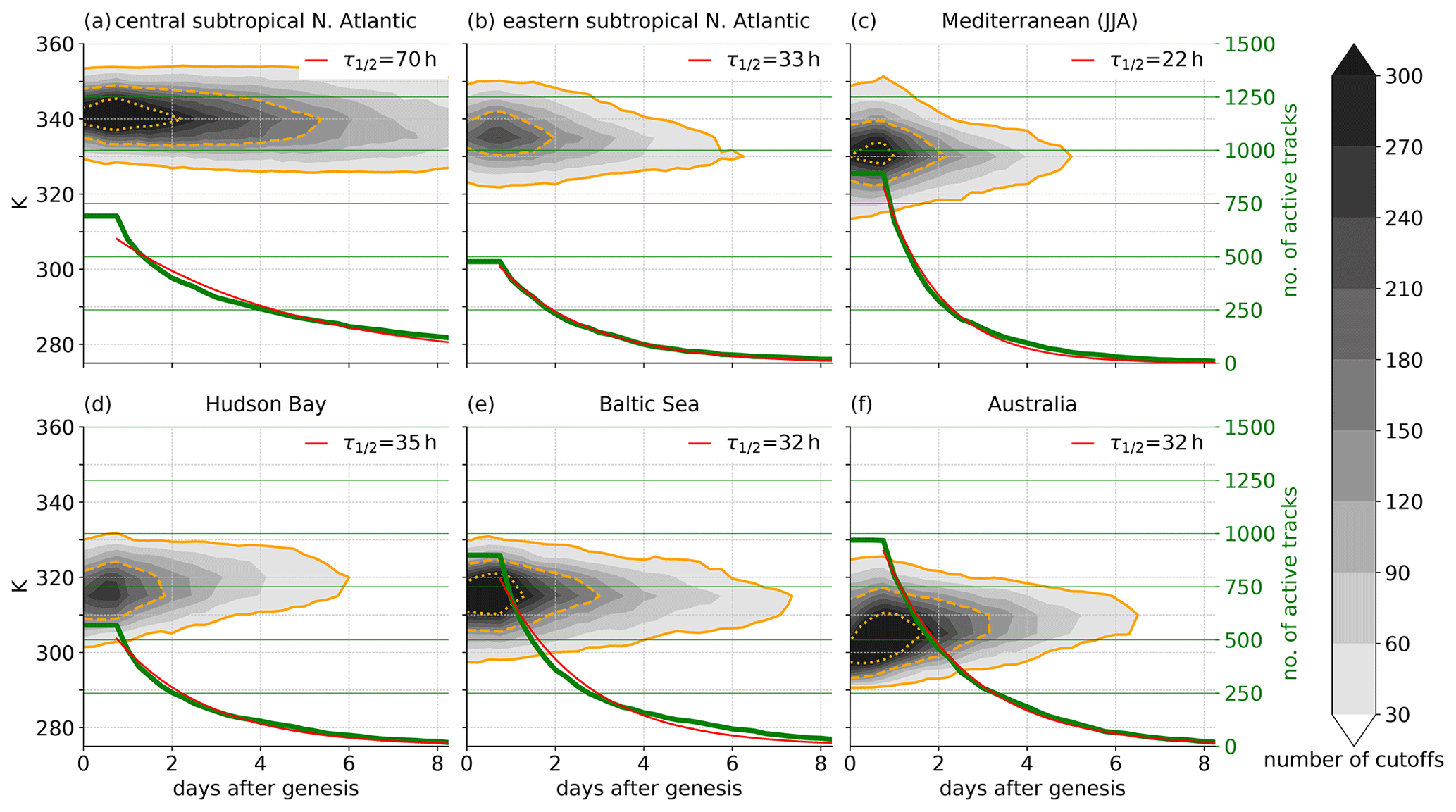
Figure 13 Same as Fig. 12 but for JJA and (a) central subtropical North Atlantic, (b) eastern subtropical North Atlantic, (c) Mediterranean, (d) Hudson Bay, (e) Baltic Sea, and (f) Australia.

In all regions, frequencies are highest about one day after genesis (Fig. 12). A main reason for this is that PV cutoffs form on a lower isentropic level first, and as the break-up of the PV streamer continues, additional vertical levels become part of the PV cutoff until it reaches its full vertical extent. Interestingly, the timescale of roughly one day until reaching the maximum extent is consistent across all regions, indicating that it can serve as an estimate of the average time required for the complete break-up of a PV streamer into PV cutoffs. In addition, for PV cutoffs over the eastern South Pacific and South Africa, the frequencies increase also below the level of maximum frequency during the first day. The only explanation for such an evolution is that these PV cutoffs grow downward, indicative of troposphere-to-stratosphere transport. On the contrary, for PV cutoffs over the Mediterranean the frequencies below the level of maximum frequency decrease rapidly, indicating diabatic decay and stratosphere-to-troposphere transport. For Antarctica, there is not much vertical displacement during the first two days, indicative of a rather adiabatic evolution.

After one day, the cutoff frequency gradually decreases in all regions, and the number of cutoff tracks that still persist at a certain time after genesis (hereafter: active tracks) follows an exponential decay relatively closely. This shows that the probability of a PV cutoff track to end is relatively constant; i.e., the lysis of PV cutoffs can be regarded as an exponential decay process. We use an exponential curve fitted to the number of active tracks to estimate the half life ${\mathit{\tau }}_{\mathrm{1}/\mathrm{2}}$ of the PV cutoffs once they have overcome the 24 h minimum duration required in this study. This value is surprisingly similar across regions and ranges from 25 h (South Africa) to 31 h (Mediterranean). Hence, the median lifetime is between 49 and 55 h and the expected (i.e., mean) lifetime $\stackrel{\mathrm{‾}}{T}$ (computed as $\stackrel{\mathrm{‾}}{T}=\mathrm{24}\mathrm{h}+{\mathit{\tau }}_{\mathrm{1}/\mathrm{2}}\cdot \ln (\mathrm{2}{)}^{-\mathrm{1}}$) between 60 and 69 h. Hence, across the regions considered, the lifetimes do not vary strongly and expected lifetimes are close to the mean lifetimes of the three cutoff types (Fig. 9a).

A similar picture appears for JJA (Fig. 13), where maximum frequencies are also found roughly one day after genesis in all regions, decaying approximately exponentially afterwards. Downward growth is also apparent for PV cutoffs over the central and eastern subtropical North Atlantic (Fig. 13a and b), while over Australia PV cutoffs rapidly disappear at lower levels (Fig. 13f). A further interesting aspect is the gradual lowering of the isentropic level with the maximum frequency along the transect of genesis regions from the central to the eastern subtropical North Atlantic and to the Mediterranean (Fig. 13a–c), consistent with an increase in latitude. Particularly noteworthy is the very large half life (70 h, $\stackrel{\mathrm{‾}}{T}=\mathrm{125}$ h) of PV cutoffs forming over the central subtropical North Atlantic, which is more than 2 times longer than in all other regions. On the contrary, PV cutoffs over the Mediterranean have a substantially shorter half life (22 h, $\stackrel{\mathrm{‾}}{T}=\mathrm{52}$ h) than in all other regions, and also than Mediterranean PV cutoffs in DJF (Fig. 12c). PV cutoffs forming over the Hudson Bay and the Baltic Sea have, similarly to PV cutoffs near Antarctica in DJF, not much vertical displacement.

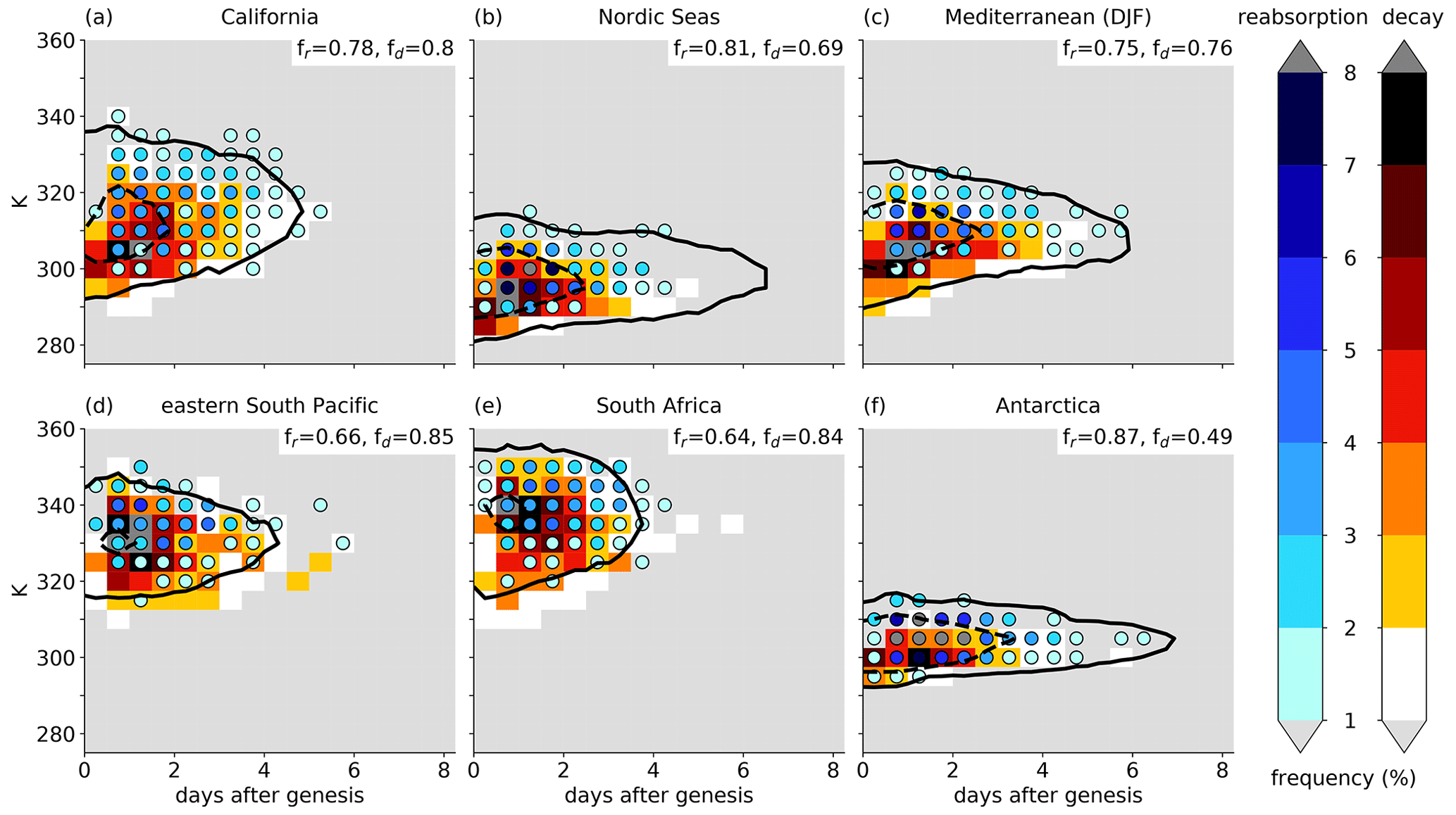
Figure 14 Relative frequency of reabsorption events (blue shaded circles, in %) and diabatic decay events (red shaded rectangles, in %) as a function of PV cutoff lifetime (binned into 12-hourly intervals) and isentropic level as well as the overall frequencies of at least one reabsorption event (f_r) or decay event (f_d) during the life cycle (numbers on top right of each panel). The climatological vertical evolution of the PV cutoffs is indicated by the black contours for (solid) 30 and (dashed) 150 cutoffs as shown in Fig. 12. Shown are the six genesis regions in DJF: (a) California, (b) Nordic Seas, (c) Mediterranean, (d) eastern South Pacific, (e) South Africa, and (f) Antarctica.

4.3 Diabatic decay and reabsorption

The climatological vertical evolution of the 3D PV cutoffs discussed in the previous section is determined by the appearance and disappearance of 2D PV cutoffs on isentropic levels. A PV cutoff appears on an isentropic level either during the break-up process or as it grows downward, involving TST. While these processes are not directly quantified in this study, the processes leading to disappearance, i.e., diabatic decay and reabsorption, are. In this section, the frequencies of diabatic decay and reabsorption are discussed for the life cycles of PV cutoffs in the selected genesis regions. As in Sect. 3.2, all disappearance events of 2D PV cutoffs with a decay fraction less than 50 % are considered as reabsorption and all other events as diabatic decay.

First, we discuss the overall frequencies with which a PV cutoff in a certain genesis region in DJF experiences at least one reabsorption event (f_r, see Fig. 14) or at least one decay event during their life cycle (f_d). They vary substantially between roughly 50 % and well above 80 % across regions. Consistent with Fig. 9d and e, cutoffs in regions where Type III (poleward of jet) dominates (Nordic Seas, Antarctica) have the highest reabsorption frequencies and the lowest decay frequencies and vice versa for regions where Type I (equatorward of jet) dominates (eastern South Pacific, South Africa). In regions with mostly Type II (between jets) cutoffs (California, Mediterranean), both scenarios occur roughly equally frequently. It is also noteworthy that the frequency with which a PV cutoff experiences at least one decay event during the life cycle is 20 percent points larger over the Nordic Seas than close to Antarctica, even if Type III dominates in both regions. This shows clearly that regional aspects are also relevant.

These overall frequencies are complemented by the vertical distributions and temporal evolution of reabsorption and diabatic decay frequencies (Fig. 14). In all regions, diabatic decay tends to occur at lower levels than reabsorption. In fact, as diabatic decay is mainly responsible for the decrease of PV cutoff frequencies (as shown in Fig. 12 and black contours in Fig. 14) below the level of maximum frequency, reabsorption rather leads to the reduction in frequencies above; hence, the combination of the two determines the climatological vertical evolution. Consistent with the exponential decay of the number of PV cutoffs after 1 d, decay and reabsorption frequencies are particularly high between about 1–2 d after genesis in all regions. However, while only a low fraction of PV cutoffs over the eastern South Pacific and South Africa experiences decay during the first 12 h after genesis, this occurs more frequently for cutoffs in the other regions. This indicates differences in the timing of diabatic activity related to the PV cutoff.

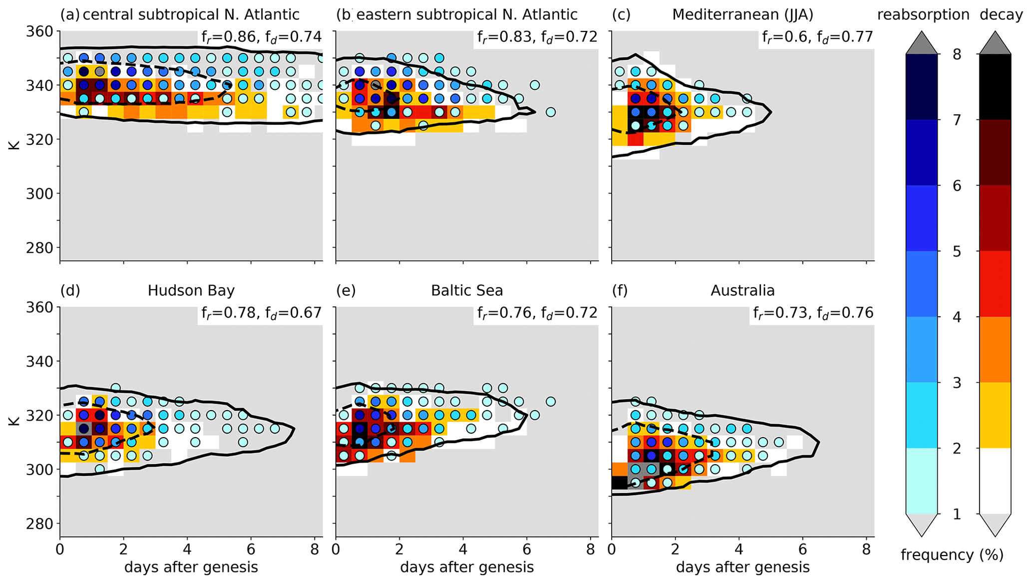
Figure 15 Same as Fig. 14 but for JJA and (a) central subtropical North Atlantic, (b) eastern subtropical North Atlantic, (c) Mediterranean, (d) Hudson Bay, (e) Baltic Sea, and (f) Australia.

In JJA (Fig. 15) the values of f_r and f_d also vary across regions. However, here, regions with the highest f_r (well above 80 %) are dominated by Type I cutoffs (central and eastern subtropical North Atlantic), which is significantly higher than the climatology of Type I (f_r=66 %). PV cutoffs over the Mediterranean, which are also dominated by Type I, have a lower f_r of 60 %. Noteworthy is also the significantly lower f_r of PV cutoffs over the Mediterranean in summer than in winter, consistent with the climatological differences between Types I and II.

The vertical distributions and temporal evolutions of decay and reabsorption frequencies show in JJA a similar general pattern as in DJF with a tendency for decay to occur at lower levels and reabsorption at higher levels. Both scenarios are particularly frequent between 1–2 d lifetime. Reabsorption rarely occurs during the first 12 h while, in some regions, decay is already quite frequent initially. This is likely the case because PV cutoffs are still in the break-up stage. Unexpected are the frequent decay events on 335 K for PV cutoffs over the central subtropical North Atlantic (Fig. 15a), as at the same time the cutoff frequency at this level remains fairly constant. This indicates that the many decay events must be compensated by the downward extension (i.e., many appearances), such that, on average, these PV cutoffs do not decay on 335 K during several days.

4.4 Link to surface cyclones

Finally, we analyze the link of PV cutoffs to surface cyclones in the different genesis regions. Similarly to Sect. 3.3 and with the approach described in Sect. 2.5, we identify situations where PV cutoffs are located near surface cyclones and ask the following: how frequently are PV cutoffs linked to a surface cyclone in the different regions? In addition, we analyze how this frequency changes with the lifetime of the PV cutoff. Finally, we investigate how PV cutoff life cycles and cyclone life cycles are temporally linked, e.g., address the following questions: does cyclogenesis occur before or after PV cutoff genesis? If it occurs afterwards, does it occur in the vicinity of the PV cutoff? Answering these questions will provide information not only on how the surface impact of PV cutoffs varies across regions, but also on how PV cutoff life cycles are linked to the life cycle of the low-level baroclinic wave signal in the different regions.

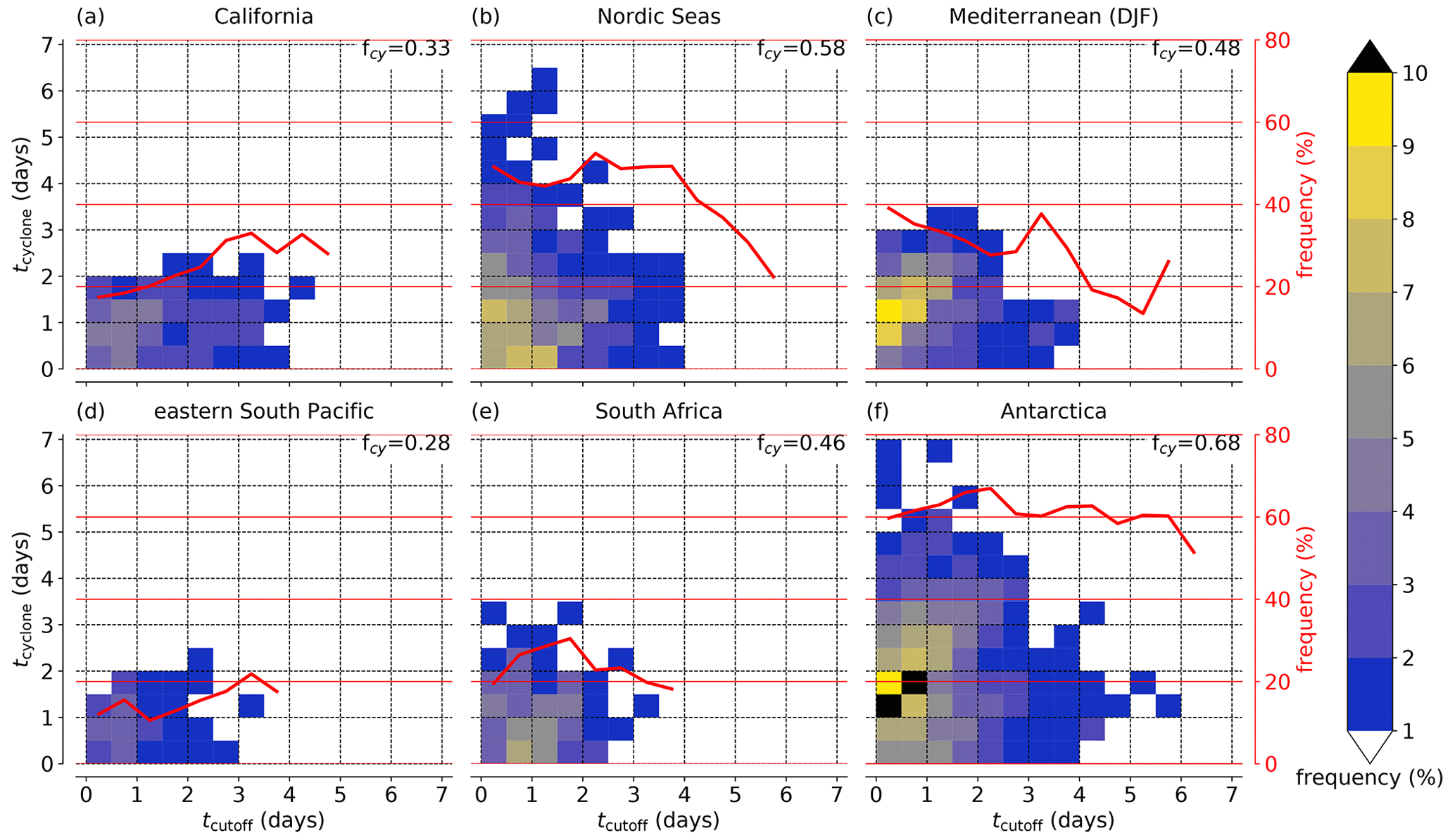
Figure 16 Relative frequencies of PV cutoffs linked to a surface cyclone (shading, in %) as a function of cutoff lifetimes (t_cutoff) on the horizontal axis and surface cyclone lifetimes (t_cyclone) on the vertical axis, binned into 12-hourly time intervals. The red contour shows the relative frequency of cutoffs linked to surface cyclones as a function of cutoff lifetime, e.g., the value at day 3 indicates the percentage of PV cutoffs with a lifetime of at least 3 d that are linked to a surface cyclone at day 3. PV cutoffs positioned in the lowermost row of the diagram are linked to a surface cyclone within 12 h after surface cyclogenesis, and PV cutoffs positioned in the leftmost column of the diagram are linked to a surface cyclone within 12 h after PV cutoff genesis. The relative frequencies of PV cutoffs with at least one link to a surface cyclone during their life cycle are indicated at the top right in each panel (f_cy). Shown are results for PV cutoffs with genesis in DJF in the regions: (a) California, (b) Nordic Seas, (c) Mediterranean, (d) eastern South Pacific, (e) South Africa, and (f) Antarctica.

Figure 16 provides the relevant information for the genesis regions in DJF. The frequencies with which a PV cutoff is linked to a surface cyclone during its life cycle (f_cy) varies strongly across regions, mostly consistent with Fig. 8 and the dominant cutoff types in each region. PV cutoffs over the Nordic Seas and Antarctica (Fig. 16b and f), i.e., in storm track regions, are linked to surface cyclones in 58 % and 68 % of the cases, which is even higher than the climatological value for Type III (poleward of jet). The lowest frequencies (28 %–33 %), albeit well above the climatological value of Type I (equatorward of jet), occur for cutoffs over the eastern South Pacific and California. PV cutoffs over the Mediterranean and South Africa have intermediate frequencies, close to the climatological frequency of Type III. The high frequencies for PV cutoffs over South Africa (46 %) are noteworthy as many of them are Type I cutoffs, which, climatologically, are only rarely linked to surface cyclones. The generally higher frequencies compared to what could be expected from the climatological frequencies of the dominant type in each region indicate that in the considered regions cutoffs are particularly relevant for surface cyclones.

The frequency of PV cutoffs linked to surface cyclones as a function of lifetime increases over California, the eastern South Pacific, South Africa, and Antarctica during the first couple of days (red curves in Fig. 16a, d, e, and f). This shows that PV cutoffs linked to surface cyclones are particularly long-lived. Because PV cutoffs that are initially linked to surface cyclones are not exceptionally long-lived (not shown), an explanation could be that longer-lived PV cutoffs result in cyclogenesis later during their life cycle. This reason could also explain why the frequency of PV cutoffs forming over the Nordic Seas and in particular the Mediterranean initially decreases but shows a secondary peak after 2 and 3 d, respectively (Fig. 16b and c).

This aspect can be partly resolved by counting all PV cutoffs that are at lifetime t_cutoff linked to a surface cyclone at lifetime t_cyclone and show these frequencies in a t_cutoff vs. t_cyclone diagram (shading in Fig. 16). For example, the yellow and black colors in the leftmost column in Fig. 16f show that, at their genesis, about 20 % of the PV cutoffs close to Antarctica are linked to surface cyclones that are between 1–2 d old. The diagonal displacement of these yellow colors for higher PV cutoff lifetimes indicates that the PV cutoffs remain linked to the surface cyclones, and the two propagate and become older together. The transition to blue colors along this diagonal shows that the number of these initial links decreases with time. A link disappears either because the PV cutoff decays, the surface cyclones decays, or the surface cyclone and the PV cutoff move away from each other. As another example, the yellowish boxes in the lowermost row in Fig. 16e show that about 10 % of the PV cutoffs with genesis over South Africa are related to surface cyclogenesis after a cutoff lifetime of 0.5–1.5 d (as indicated by the sum of the values in the 0.5–1 and the 1–1.5 d boxes in the lowermost row).

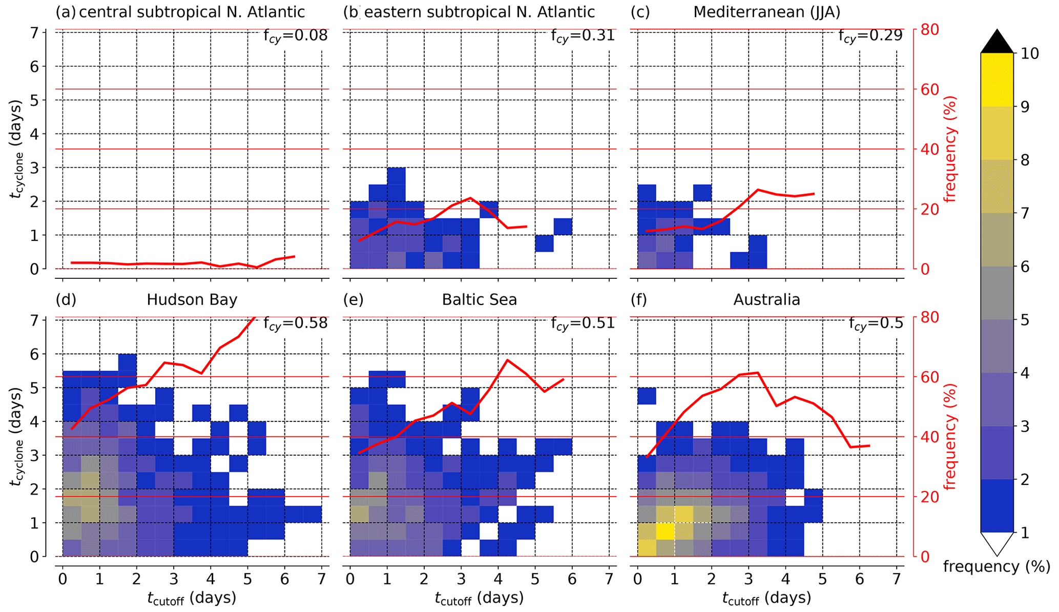
Figure 17 Same as Fig. 16 but for PV cutoffs in JJA with genesis in the regions: (a) central subtropical North Atlantic, (b) eastern subtropical North Atlantic, (c) Mediterranean, (d) Hudson Bay, (e) Baltic Sea, and (f) Australia.

Cyclogenesis in the vicinity of the PV cutoff after up to 4 d lifetime occurs in all regions and can partly explain the increases or local peaks in the fraction of PV cutoffs linked to surface cyclones during their lifetime. In general, the preferred timing of PV cutoff life cycles and surface cyclone life cycles differs across regions. For example, over the Mediterranean, the most frequent scenario is that surface cyclones form between 0.5–1.5 d prior to PV cutoff genesis and remain linked to the PV cutoff for about 1–2 d. Similarly, PV cutoffs close to Antarctica are often linked to surface cyclones that form 1–2 d prior to PV cutoff genesis. For cutoffs over the Nordic Seas, scenarios with cyclogenesis between about 2 d prior and 1.5 d after PV cutoff genesis are all roughly equally frequent. And the most frequent scenario for PV cutoffs forming over South Africa is cyclogenesis in the vicinity of the PV cutoff between 0.5–1.5 d after PV cutoff genesis. Hence, over South Africa, cyclogenesis occurs as a consequence of the PV cutoff, while over the Mediterranean and Antarctica, PV cutoff formation is rather the result of surface cyclogenesis and associated in situ baroclinic development. The latter scenario is consistent with the classical picture of the LC2 evolution and the composite of Type III cutoffs (Fig. 8c and f), which shows a well-developed surface cyclone at PV cutoff genesis (see also the case shown in Fig. S4). But also secondary cyclogenesis ahead of an equatorward extended PV streamer forming downstream of an LC1 evolution and subsequent cyclonic break-up may result in a situation where PV cutoff genesis follows or co-occurs with surface cyclogenesis (as it can occur for Type II (between jets) cutoffs, see Fig. 8b and e and associated discussions and Fig. S3).

Also in JJA, the different regions show distinct characteristics (Fig. 17). The relative frequency of PV cutoffs linked to a surface cyclone during the life cycle ranges between 8 % over the central subtropical North Atlantic to 58 % over the Hudson Bay. It is lowest for regions where Type I dominates and highest for regions where Type III dominates, consistent with the climatology of the three types. PV cutoffs forming over the Mediterranean are substantially less frequently linked to surface cyclones in JJA compared to DJF, in agreement with the seasonality of the Mediterranean storm track (e.g., Wernli and Schwierz, 2006). Surface cyclones linked to PV cutoffs over Australia frequently form almost simultaneously with the PV cutoff (Fig. 17f, consistent with a Type II evolution and the example in this region shown in Fig. S3). On the contrary, surface cyclones linked to PV cutoffs over the Hudson Bay and the Baltic Sea preferentially form up to several days prior to PV cutoff genesis (Fig. 17d and e) as it can be expected for a classical LC2 evolution that results in Type III cutoffs. In most regions, the fraction of PV cutoffs linked to a surface cyclone increases with the lifetime of the PV cutoffs during the first couple of days. Again, this can partly be linked to cyclogenesis in the vicinity of the PV cutoff after genesis, which occurs in most regions. But it can also occur that, after a couple of days, PV cutoffs meet a relatively old surface cyclone (as indicated by increases in the frequencies along a diagonal, e.g., around a t_cutoff of 4 d and a t_cyclone of 1.5 d over the Baltic Sea, Fig. 17e).

We conclude that there are general consistencies of the linkage between PV cutoffs and surface cyclones in the considered regions with archetypal baroclinic wave evolutions and the corresponding PV cutoff types. However, the wide range of combinations of PV cutoff lifetimes and cyclone lifetimes that can occur when the two systems meet shows that potentially complex evolutions take place. Further, the substantial differences between regions with the same dominant cutoff type show that specific local processes (such as, e.g., orographic influence on cyclogenesis) may play an important role.

5 Summary and conclusions

In this study, a novel approach to identify and track PV cutoffs as three-dimensional objects was introduced and applied to ERA-Interim reanalyses for the years 1979–2018. This climatology of PV cutoffs is the first that comprises all near-tropopause cyclonic vortices, because it is global and independent of the selection of a vertical level. As the tracking is based on isentropic trajectories, it further allows quantifying diabatic decay and reabsorption. The resulting climatological dataset was used to study the life cycle of PV cutoffs in detail. In the following, a summary of the main results is given, separated into the three overarching findings, which are (1) new insight into climatological occurrence and frequencies of decay and reabsorption, (2) a meaningful classification into three PV cutoff types, and (3) substantial regional variability of PV cutoff life cycles and relevance of their vertical dimension. Finally, a brief outlook for further research is given.

Table 1 Characteristics of the three PV cutoff types.

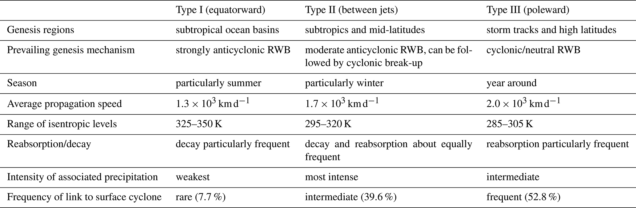
5.1 New insight into climatological frequencies, decay, and reabsorption

Many of the presented frequency, genesis, and lysis maxima of PV cutoffs are consistent with previous climatological studies, but some previously unknown regions of occurrence are identified (e.g., the circumpolar band around Antarctica). A main novelty of this study is that all of them are identified based on a consistent methodology and independent of the selection of a vertical level, providing the most comprehensive climatological picture of PV cutoffs so far. It reveals that PV cutoffs in summer occur frequently over subtropical ocean basins equatorward of the jet stream, and at higher latitudes, in particular in the storm track regions poleward of the jet stream. In winter, PV cutoffs occur either poleward of the jet stream or, particularly frequently, in regions with split-jet conditions between the polar and subtropical jet streams.

Further, the first climatological quantification of diabatic decay and reabsorption revealed that both scenarios occur equally frequently, in contrast to the prevailing opinion that diabatic decay dominates. While decay tends to occur on lower isentropic levels, reabsorption is more frequent on higher isentropic levels. In addition, we found that the two scenarios have distinct geographical patterns of occurrence. This novel analysis sheds new light into a fundamental aspect of dynamical meteorology. In addition, the frequent occurrence of reabsorption may be relevant for midlatitude predictability, because it is a nonlinear interaction of the PV cutoff and the PV waveguide that potentially results in large uncertainties in the Rossby wave pattern (see, e.g., Baumgart and Riemer, 2019).

5.2 Meaningful classification into three PV cutoff types

Following Bell and Bosart (1989) and Price and Vaughan (1992), we classified PV cutoffs according to their position relative to the jet stream (Type I: equatorward, Type II: between two jets, Type III: poleward). We argue that such a classification is meaningful from both a fundamental atmospheric dynamics as well as from a predictability and impacts perspective. The main characteristics of the three types are summarized in Table 1.

From a fundamental atmospheric dynamics perspective, the results show that PV cutoff life cycles can be linked to the well-established archetypes of baroclinic wave life cycles and Rossby wave breaking. Type I forms in the subtropics from anticyclonic Rossby wave breaking and can be regarded as the result of an LC1 type evolution. Type III forms mainly in the storm track regions from cyclonic RWB, which is consistent with an LC2 type evolution. Finally, Type II forms in the subtropics and mid-latitudes and, similarly to Type I, from anticyclonic RWB. But, on the contrary to Type I, it forms in an area with cyclonic barotropic shear equatorward of a (subtropical) jet stream, which counteracts the anticyclonic tilt and can result in a cyclonic break-up of the PV streamer. While pointing out these consistent dynamical scenarios, we also recognize the large variability within each type and that individual evolutions may substantially differ from these archetypes. Nonetheless, the classification may provide helpful guidance to study the predictability and surface impacts of PV cutoffs. It stresses that particular attention should be given to Type II cutoffs, because of their potentially substantial impact on surface cyclogenesis and precipitation and their frequent occurrence in populated areas. In addition, given the different dynamical situations that lead to the formation of the three types, substantial differences in the processes influencing their predictability can be expected. For example, for Type III, errors in the surface cyclogenesis process prior to PV cutoff genesis may be a major driver of errors related to the PV cutoff. Such an influence is not expected for Type I, because they are rarely close to surface cyclones. On the contrary, errors related to anticyclonic RWB and/or the upstream surface cyclone might be particularly relevant for errors related to Type I and II cutoffs (similar to the cases discussed in, e.g., Pantillon et al., 2013, and Portmann et al., 2020).

5.3 Substantial regional variability of PV cutoff life cycles and relevance of their vertical dimension

In the second part, subsets of PV cutoff tracks were selected based on 12 different genesis regions, and their tracks, vertical evolution, decay and reabsorption, and the link to surface cyclones were studied in detail.

A particularly novel aspect was a composite analysis of the vertical evolution of PV cutoffs along the life cycle, which highlighted the relevance of the vertical dimension when investigating PV cutoffs. It showed that PV cutoffs can extend over many isentropic levels and in different regions exhibit different climatological vertical “footprints” during their life cycles. While some tend to rise to higher levels, others tend to sink to lower levels. Remarkably consistent across regions is the average duration of about one day until the climatological maximum vertical extent is reached, i.e., until the full three-dimensional break-up process is completed after PV cutoff genesis.

These vertical footprints of PV cutoffs are modulated by the appearance and disappearance of PV cutoffs on single isentropic levels. The relative frequency with which a PV cutoff undergoes diabatic decay or reabsorption during its life cycle varies greatly between regions. Interestingly, in some regions, these frequencies are substantially different from the climatological frequencies of the dominant PV cutoff type in the respective region. This demonstrates that the probability of a PV cutoff to experience diabatic decay or reabsorption can be strongly influenced by specific regional characteristics.

On the contrary, it is found that the expected lifetimes are relatively similar across most regions, with the notable exception of PV cutoffs forming over the cental subtropical North Atlantic, which persist on average more than twice as long as in most other considered regions.

Considering the link to surface cyclones we found that the frequency with which a PV cutoff is linked to a surface cyclone during its life cycle strongly depends on the region and that these differences cannot only be explained with the climatological differences between the cutoff types, additionally suggesting that regional aspects matter. By analyzing the frequencies of the possible combinations of PV cutoff lifetimes and lifetimes of the linked surface cyclones, it was found that most regions have certain combinations that preferentially occur. In regions with many Type II and III cutoffs, surface cyclones frequently form at or up to a few days prior to PV cutoff genesis, consistent with the archetypal evolutions associated with these two PV cutoff types. As an important novel finding, they are frequently involved in surface cyclogenesis up to several days after they have formed. This highlights that, while PV cutoffs have mostly been considered as weather systems at the end of a baroclinic life cycle, they can also be initiators of new baroclinic life cycles.

5.4 Outlook

The tracking methodology and the PV cutoff climatology presented in this study open various opportunities for further research on this relevant flow feature. A major advantage is that they can be used for global studies, regional studies, and, as a particular asset, studies to compare PV cutoffs in different regions.

An interesting open question that can be addressed with the present dataset is for example how many of the identified surface cyclogenesis events linked to a PV cutoff can be reasonably explained by the dynamical forcing of the PV cutoff and how this aspect compares across regions and/or PV cutoff types. An aspect that we will address in a forthcoming study is the role of PV cutoffs for (extreme) precipitation on a global scale. A related topic may be to quantify trends in PV cutoff frequencies and the link to precipitation trends (as for example investigated for Australia by Lavender and Abbs, 2013). This would potentially contribute to the discussion about the role of dynamic and thermodynamic drivers of precipitation changes (e.g., Pfahl et al., 2017). Also, the role of particularly long-lived subtropical PV cutoffs (e.g., over the central subtropical North Atlantic) for the export of tropical moisture into the mid-latitudes and subsequent heavy precipitation events (as shown by Piaget et al., 2015, for a case study) could be investigated.

Applying the presented methodology to other datasets even opens doors to answering further relevant questions. For example, using climate model simulations it could be studied how the life cycles of PV cutoffs change under global warming. As it considers the full three-dimensional evolution of PV cutoffs, the methodology is also particularly useful to study errors and uncertainty in the structure and evolution of PV cutoffs in operational weather forecasts.