Subseasonal precipitation forecasts of opportunity over central southwest Asia

Subseasonal forecasts of opportunity (SFOs) for precipitation over southwest Asia during January–March at lead times of 3–6 weeks are identified using elevated expected forecast skill from a linear inverse model (LIM), an empirical dynamical model that uses statistical relationships to infer the predictable dynamics of a system. The expected forecast skill from this LIM, which is based on the atmospheric circulation, tropical outgoing longwave radiation, and sea surface temperatures, captures the predictability associated with many relevant signals as opposed to just one. Two modes of variability, El Niño–Southern Oscillation (ENSO) and the Madden–Julian Oscillation (MJO), which themselves are predictable because of their slow variations, are related to southwest Asia precipitation SFOs. Strong El Niño events, as observed in 1983, 1998, and 2016, significantly increase the likelihood by up to 3-fold of an SFO 3–4 and 5–6 weeks in advance. Strong La Niña events, as observed in 1989, 1999, 2000, also significantly increase the likelihood of an SFO at those same lead times. High-amplitude MJO events in phases 2–4 and 6–8 of greater than one standardized departure also significantly increase the likelihood of an SFO 3–4 weeks in advance. Predictable atmospheric circulation patterns preceding anomalously wet periods indicate a role for enhanced tropical convection in the South Pacific convergence zone (SPCZ) region, while suppressed convection is observed preceding predictable dry periods. Anomalous heating in this region is found to distinguish wet and dry periods during both El Niño and La Niña conditions, although the atmospheric circulation response to the heating differs between each ENSO phase.

1 Introduction

Precipitation over central southwest Asia, defined here as 22–48^∘ N, 50–80^∘ E and encompassing Afghanistan, Pakistan, Iran, Turkmenistan, Uzbekistan, Tajikistan, and Kyrgyzstan, occurs mainly during the cold season from November–April and determines the region's subsequent water supply used for agriculture and consumption (Agrawala et al., 2001; Barlow et al., 2006). It is in this context that accurate precipitation predictions are critical, given the effect of water on food security and livelihoods (Famine Early Warning Systems Network, 2022) in this semi-arid region (Barlow et al., 2016). However, precipitation forecasts from dynamical models lack skill by lead times of 3 weeks over southwest Asia (de Andrade et al., 2018; Pegion et al., 2019). An alternative endeavor is identifying the smaller subset of forecasts at lead times of 3 to 6 weeks that are skillful, so-called “subseasonal forecasts of opportunity” (SFOs; Lang et al., 2020; Mariotti et al., 2020), by forecasting the forecast skill (Kalnay and Dalcher, 1987). SFOs can arise from slowly evolving tropical phenomena such as the El Niño–Southern Oscillation (ENSO; Newman et al., 2003; Johnson et al., 2014; Domeisen et al., 2019; Mariotti et al., 2020; Albers and Newman, 2021) and Madden–Julian Oscillation (MJO; Rodney et al., 2013; Johnson et al., 2014; Li and Robertson, 2015; Mayer and Barnes, 2021), which can force atmospheric circulation patterns to the extratropics through anomalous divergence (e.g., Sardeshmukh and Hoskins, 1988).

Precipitation over southwest Asia may be a favorable target variable and location for SFOs, as both ENSO (Barlow et al., 2002; Nazemosodat and Ghasemi, 2004; Hoell et al., 2012, 2014a, b, 2015a, b, 2017, 2018a) and the MJO (Barlow et al., 2005; Nazemosodat and Ghaedamini, 2010; Hoell et al., 2013; Cannon et al., 2017; Hoell et al., 2018b) can modulate precipitation in this region. Hoell et al. (2018a) considered the sensitivity of southwest Asian precipitation to central Pacific (CP) and eastern Pacific (EP) El Niño and La Niña conditions and found that while both CP and EP El Niño conditions shifted precipitation anomalies towards the upper tercile, a wide range of extreme precipitation outcomes was still possible. CP La Niña events shifted precipitation towards the lower tercile, while EP La Niña events did not significantly shift precipitation in the region. Hoell et al. (2018b) found that, in the 5 d following MJO phases 2–4 (enhanced eastern Indian Ocean convection), negative precipitation anomalies developed as a response to an anomalous upper-level anticyclone and subsidence. Conversely, MJO phases 6–8 (suppressed eastern Indian Ocean convection) were associated with anomalous upper-level troughing, ascent, and positive precipitation anomalies. However, Cannon et al. (2017) found a nuanced impact of the MJO on extreme western Himalayan snowfall due to competing influences of the MJO on the dynamic forcing for vertical motion and moisture availability. The convolved impact of ENSO and MJO activity on precipitation in the region is cited as an additional confounding factor that can obscure the nature of the two teleconnections (Schrage et al., 1999; Hoell et al., 2013; Riddle et al., 2013). Objective methods for considering this combined influence, as well as how it leads to SFOs, are therefore of interest to both better provide real-time subseasonal forecast guidance and understand sources of predictability.

Based on past success, this study uses a linear inverse model (LIM; Penland and Sardeshmukh, 1995) and its associated signal-to-noise metric “expected skill” (Sardeshmukh et al., 2000; Newman et al., 2003) to anticipate SFOs over southwest Asia. Albers and Newman (2019) used expected skill to identify SFOs, at the time of forecast, for North Pacific and North Atlantic 500 hPa geopotential height anomalies. They found that periods of elevated expected-skill forecast by the LIM identified more skillful forecasts compared to the European Centre for Medium-Range Weather Forecasts (ECMWF) Integrated Forecasting System (IFS) and National Centers for Environmental Prediction Climate Forecast System Version 2 (NCEP CFSv2) initialized forecast systems, implying that sources of predictability are common among various model types. Albers and Newman (2021) found that North Atlantic Oscillation (NAO) SFOs could be identified in both the LIM and the IFS and were driven by a set of ENSO-related climate modes, reflecting the utility of the LIM in targeting regional phenomena.

Global processes and their unique interactions with local precipitation and temperature ultimately produce SFOs and can be identified by training a LIM on specific regional- and/or large-scale interactions, as demonstrated in Breeden et al. (2022) and Albers et al. (2022) for North American 2 m temperature (2mT). Based on these results, here we develop a LIM for subseasonal precipitation over southwest Asia that has been designed in a similar manner. We will show that precipitation SFOs determined using LIM expected skill can successfully be identified for subseasonal precipitation over southwest Asia with a LIM that is regional in precipitation and temperature but large-scale with the inclusion of hemispheric tropical outgoing longwave radiation (OLR), sea surface temperatures (SSTs), and 200 hPa Northern Hemisphere streamfunctions (Ψ₂₀₀). Another beneficial quality of the LIM is the negligible computational power needed to generate a long record of hindcasts. This study will focus on LIM SFOs and does not evaluate the skill of other models, though past research suggests that forecasts generated elsewise can similarly be more skillful during LIM-identified SFOs (Albers and Newman, 2019, 2021).

The LIM developed for regional precipitation over southwest Asia is used to test the hypothesis that SFOs can be anticipated using theoretical expected skill and are associated with strong ENSO and MJO events. Section 2 introduces the reanalysis and satellite products employed, how the LIM is constructed, and how SFOs are identified using expected skill. Section 3 shows a comparison of this approach to other methods of anticipating periods of elevated forecast skill, as well as the correspondence between forecasts of opportunity and ENSO and the MJO. Section 4 contextualizes results and proposes next steps.

2 Data and methods

2.1 Data

To train the LIM, Ψ₂₀₀, 2mT, SST, and OLR data from Japan Meteorological Agency 55-year Reanalysis (JRA-55; Kobayashi et al., 2015) and precipitation from the Climate Hazards group Infrared Precipitation with Stations (CHIRPS; Funk et al., 2015) dataset are used for the period January–March in 1982–2020. Variables and their respective domains are listed in Table 1. To consider how forecast skill and forecasts of opportunity change as a function of the ENSO phase, the Niño3.4 index was calculated using SST anomalies averaged from 5^∘ N–5^∘ S, 170–120^∘ W (Trenberth, 1997; Trenberth and Stepaniak, 2001). For examining relationships between skill and the MJO, the real-time multivariate MJO (RMM) index, a combined tropical OLR and circulation index that is designed to capture characteristics of the MJO (Wheeler and Hendon, 2004), is employed, including RMM amplitude, which measures MJO strength, and each day's associated MJO phase, which tracks MJO location. Finally, based on results in Sect. 3b, we assess the strength of tropical OLR anomalies in the South Pacific convergence zone (SPCZ; box in Fig. 10), defined as 10^∘ S–2.5^∘ N, 140–180^∘ E. The time series of OLR anomalies in this region is considered a third metric, in addition to Niño3.4 and RMM, that might increase the likelihood of an SFO occurring.

Table 1 LIM variables that compose the state vector x, their domain, and the percent (%) variance explained by the retained empirical orthogonal functions (EOFs). Variables include the 200 hPa streamfunction (Ψ₂₀₀), the 2 m temperature (2mT), the sea surface temperature (SST), and outgoing longwave radiation (OLR). Precipitation (Precip) from the Climate Hazards group Infrared Precipitation with Stations (Funk et al., 2015) Version 2.0 dataset (https://data.chc.ucsb.edu/products/CHIRPS-2.0/, last access: 21 October 2021) is also used. JRA-55 and CHIRPS are used because they are available in near real time (2–3 d lag) and serve as the basis for experimental real-time forecasts and because they are available back to at least 1982. Ψ₂₀₀, SST, and OLR anomalies are used on a 2.5 × 2.5^∘ horizontal grid, while 2mT and Precip are used on a 0.5 × 0.5^∘ grid. The EOFs and principal components (PCs) retained in x are not sensitive to the gridding used (not shown).

2.2 Linear inverse model

A LIM assumes that the evolution of a subset of climate anomalies, defined in the state vector x, can be approximated as the sum of a slowly evolving, potentially predictable component and a rapidly decorrelating, unpredictable component. Here we consider the evolution of the following climate variables (Eqs. 1–2; Table 1):

$$\begin{array}{}\text{(1)}& {\displaystyle }\mathbf{x}=\mathit{\{}\mathrm{SST},\mathrm{OLR},{\mathrm{\Psi }}_{\mathrm{200}},\mathrm{2}\mathrm{mT},\mathrm{Precip}\mathit{\}},\text{(2)}& {\displaystyle \frac{\mathrm{d}x}{\mathrm{d}t}}=\mathbf{Lx}+{\mathbf{F}}_{\mathrm{s}},\end{array}$$

where the dynamic operator L represents the predictable component of the evolution and F_s represents state-independent white noise forcing that is unpredictable. The LIM employed in this study is created using an L designed to capture “slow and predictable” weekly-timescale variability, as in past studies (Winkler et al., 2001; Newman et al., 2003; Albers and Newman, 2019; Breeden et al., 2020; Henderson et al., 2020). Any predictable processes represented by the variables in x are aggregated in the operator L, and their net effect on the predictable evolution of the system is leveraged in the LIM (i.e., ENSO/MJO variability). To the extent the key predictable relationships between the LIM variables, whether truly linear or nonlinear, can be estimated linearly through the covariance between model variables (Eq. 3), they can be represented by L. As such, the LIM can include more information than what is retained in models based on the linearized equations of motion that explicitly exclude nonlinear effects.

Consistently with focusing on the predictable, weekly varying component of the system evolution, the climate anomalies used in the LIM were calculated by removing the 40-year daily climatology and then applying a 7 d mean. Practically, one cannot use anomalies occurring after the initialization date to make a forecast, so instead of a centered 7 d mean, the prior 6 d is averaged with the initialization date's anomalies to create the 7 d running-mean anomalies. Many variable combinations and regional domains were tested, and the combination used here was found to produce the highest precipitation forecast skill during SFOs over southwest Asia. Since the leading empirical orthogonal functions (EOFs) retained in x are not sensitive to small changes in the 2mT and Precip domains selected, LIM forecasts and SFOs are also not sensitive to small changes in the regional domains. Note that the influence of variables that are not explicitly included in this LIM, for instance slowly evolving soil moisture, can still be implicitly included in the LIM variables, such as 2mT.

The instantaneous C₀ and 5 d lagged covariance ${\mathbf{C}}_{{\mathit{\tau }}_{\mathrm{o}}}$ between the state vector components are used to determine L:

$$\begin{array}{}\text{(3)}& \mathbf{L}=\ln \left({\mathbf{C}}_{{\mathit{\tau }}_{\mathrm{o}}}\times \mathrm{inv}\left({\mathbf{C}}_{\mathrm{0}}\right)\right)/{\mathit{\tau }}_{\mathrm{o}}.\end{array}$$

As a practical consideration to reduce the dimensionality of L, each variable in x is truncated using EOF analysis, where enough EOFs are retained to capture most of the variance in each variable and region (Table 1). The covariance and lagged covariance are then computed using the principal components that are retained.

A specific training lag τ_o must be selected to compute the lagged covariance. If the system were perfectly linear and forced by white noise, L would not be sensitive to the training lag, but in practice there are constraints on the range of training lags that are appropriate, which is determined using the “τ test” (Penland and Sardeshmukh, 1995). For this LIM, a training lag of 5 d is used, which is consistent with the range of stable training lags for LIMs similar to the one used here (Winkler et al., 2001; Newman et al., 2003; Breeden et al., 2020; Henderson et al., 2020). For further information on the sensitivity of weekly LIMs to training lag and additional parameters, the reader is referred to Sect. 5 of Winkler et al. (2001).

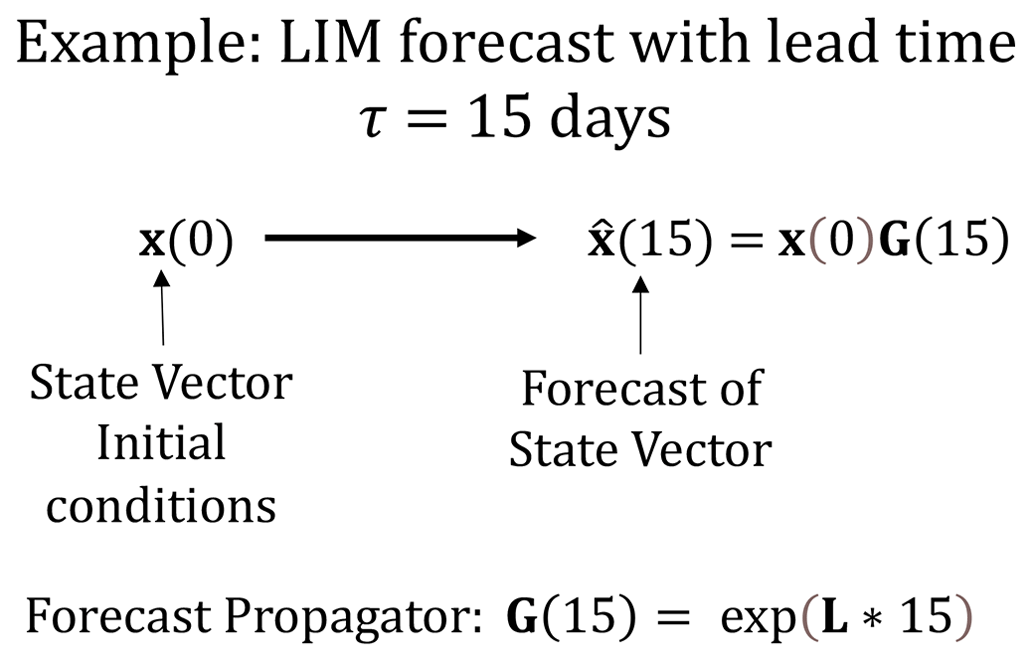
Similarly to output from numerical forecast models, for each initialization and lead time τ, the LIM generates forecasts of the state vector, $\widehat{\mathbf{x}}\left(\mathit{\tau }\right)$ (Eq. 4; Fig. 1), by propagating the initial conditions x(0) forward in time. In the LIM, the propagator G(τ) is determined from L by solving the homogeneous component of Eq. (2) (Penland and Sardeshmukh, 1995). For this study, forecasts are generated at a daily time step out to a lead time of 42 d. We note that because the LIM is trained on daily anomalies with a 7 d running mean applied, the forecasts are also lower-frequency in nature.

$$\begin{array}{}\text{(4)}& \widehat{\mathbf{x}}\left(\mathit{\tau }\right)=\mathbf{x}\left(\mathrm{0}\right)\exp \left(\mathbf{L}\mathit{\tau }\right)=\mathbf{x}\left(\mathrm{0}\right)\mathbf{G}\left(\mathit{\tau }\right)\end{array}$$

LIM forecast skill is assessed using 10-fold cross-validation, done by removing 10 % of the data, re-computing L, and generating forecasts for the 10 % of initializations that were removed (e.g., Albers and Newman, 2019). This process is repeated to generate forecasts for 1982–2020, initialized daily from 1 January–20 March each year. LIM forecast skill is assessed in two ways: using the anomaly correlation coefficient (ACC), where the LIM forecast and un-truncated (i.e., full-field) verification precipitation is compared at each grid point, and using the pattern correlation coefficient (PCC), where the LIM forecast and un-truncated verification precipitation are compared at each time step using the uncentered, cosine-weighted correlation between all grid points over southwest Asia (e.g., Albers and Newman, 2019). The ACC measures skill over the full period while preserving geographic information about skill, while the PCC measures the average skill over the entire southwest Asian domain but maintains information about how individual forecasts performed. Average forecasts using different lead times are categorized as follows: week 1 forecast lead times 1–7 d, week 2 forecast lead times 8-14 d, week 3 forecast lead times 15–21 d, week 4 forecast lead times 22–28 d, week 5 forecast lead times 29–35 d, and week 6 forecast lead times 36–42 d. Weeks 3–4 and weeks 5–6 forecasts are determined using the corresponding 14 d averaged forecasts at the corresponding lead times.

Figure 1 Schematic of LIM forecast for a lead time of 15 d.

2.2.1 Forecasts of opportunity

A common approach to anticipate SFOs is to focus on a specific predictability source, e.g., strong tropical heating associated with ENSO or the MJO. However, many potentially predictable signals may be evolving at any given time (Albers et al., 2022), and the constructive or destructive interference between each signal's teleconnections may enhance or degrade the overall predictable forecast signal for variables that we are interested in, e.g., southwest Asian precipitation. Thus, it is more desirable to use a method that considers all relevant signals and their combined influence to anticipate the overall likelihood of a skillful forecast over the region of interest. Here, following Sardeshmukh et al. (2000), the theoretical expected skill of a perfect, infinite ensemble member forecast, ρ_∞(τt) (Eq. 5), is selected to identify SFOs, based on the method's past success. In particular, ρ_∞ is calculated using the pattern correlation version of the LIM signal-to-noise ratio, S² (Eq. 6; Newman et al., 2003), and is evaluated over the southwest Asian domain for each forecast lead time τ and each initialization date t. As a result, S² and ρ_∞ are a function of time but not space:

$$\begin{array}{}\text{(5)}& {\displaystyle }{\mathit{\rho }}_{\mathrm{\infty }}\left(\mathit{\tau },t\right)={\displaystyle \frac{S^{\mathrm{2}}(\mathit{\tau },t)}{{\left\{\left[S^{\mathrm{2}}\left(\mathit{\tau },t\right)+\mathrm{1}\right]S^{\mathrm{2}}\left(\mathit{\tau },t\right)\right\}}^{\mathrm{0.5}}}},\text{(6)}& {\displaystyle }{S}^{\mathrm{2}}\left(\mathit{\tau },t\right)={\displaystyle \frac{\mathrm{tr}\left[\mathbf{F}\left(\mathit{\tau },t\right)\right]}{\mathrm{tr}\left[\mathbf{E}\left(\mathit{\tau }\right)\right]}}.\end{array}$$

S² is determined using F(τ,t), the forecast signal covariance matrix determined at a given lead time, which indicates the strength of the predictable signal in the forecasts, and E(τ), the forecast error covariance matrix which represents lead-dependent, unpredictable “noise”:

$$\begin{array}{}\text{(7)}& {\displaystyle }\mathbf{F}\left(\mathit{\tau },t\right)=\langle \widehat{\mathbf{x}}\left(t+\mathit{\tau }\right)\widehat{\mathbf{x}}(t+\mathit{\tau }{)}^{\prime }\rangle ,\text{(8)}& {\displaystyle }\mathbf{E}\left(\mathit{\tau }\right)={\mathbf{C}}_{\mathrm{0}}-\mathbf{G}\left(\mathit{\tau }\right){\mathbf{C}}_{\mathrm{0}}\mathbf{G}{\left(\mathit{\tau }\right)}^{\prime },\end{array}$$

where ^′ denotes the matrix transpose. Note that E is not a function of time, which is consistent with the assumption of state-independent noise (Eq. 2), but does vary with forecast lead time τ.

We define SFOs as the top 20 % of expected-skill forecasts as this subset accurately identifies significantly more skillful forecasts for a range of lead times (Fig. 2). The ACC and PCC during these dates are compared to the skill when, instead of expected skill, the top 20 % of Niño3.4 amplitude and RMM amplitude values are used to identify periods of elevated skill. The skill during these three subsets of forecasts (ρ_∞, Niño3.4, RMM) is compared to the skill of the remaining 80 % of expected-skill forecasts, and the 95 % confidence level in the skill differences during the three subsets is assessed nonparametrically, using bootstrapping with replacement. Similar skill differences were found for a range of 10 %–25 % of the forecasts in the SFO group, and 20 % was chosen because it provided the greatest number of samples – useful for further separating forecasts by ENSO and MJO phase later – but was small enough so that the subset has significantly elevated skill.

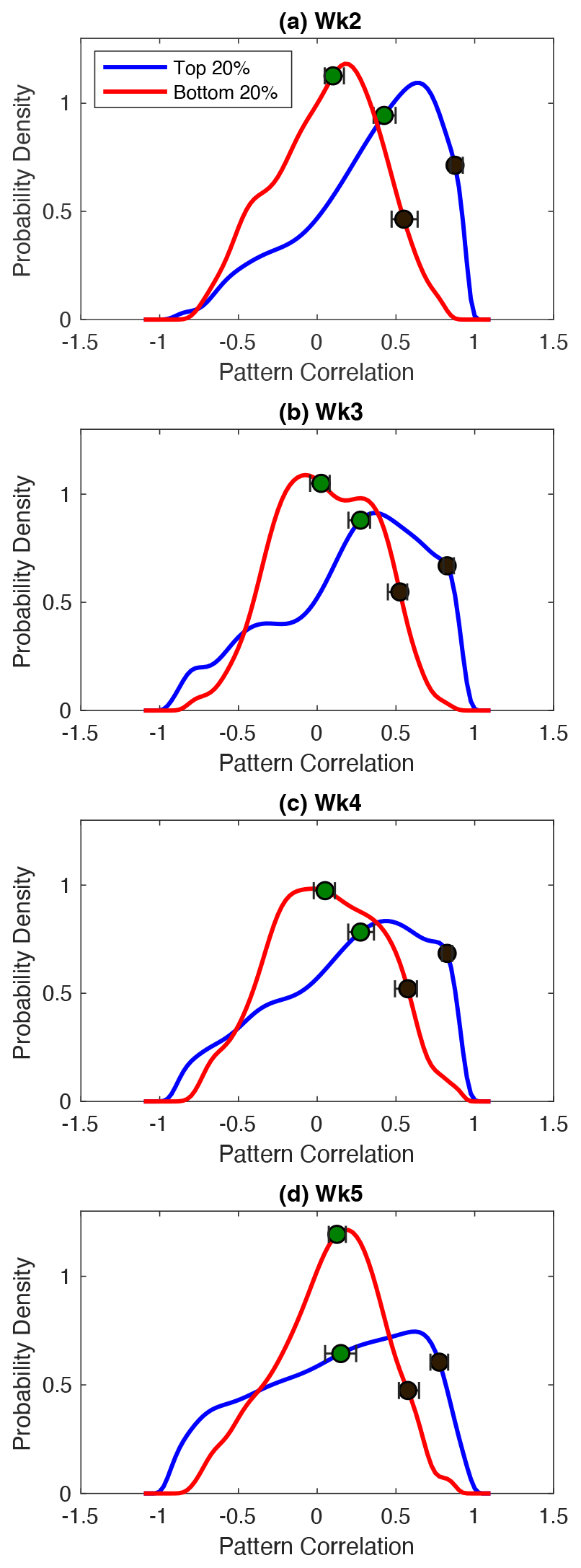
Figure 2 PDFs of actual skill measured by pattern correlation (PCC), for the top 20 % and bottom 20 % of expected-skill dates for weeks of lead times (a) 2 to (d) 5. The green circles represent the bootstrapped median values, and the black circles represent the bootstrapped 95th-percentile values.

2.2.2 Relative risk

A relative-risk ratio is used to quantify shifts in the likelihood of an SFO occurring as a function of ENSO, MJO, and SPCZ OLR strength. This is done, for each index, by determining the fraction (FRAC) of SFOs initialized on days with index values of varying amplitude:

$$\begin{array}{}\text{(9)}& \mathrm{FRAC}=\mathrm{no}.\mathrm{SFOs}/\mathrm{no}.\mathrm{dates}.\end{array}$$

For ENSO and SPCZ OLR, changes in SFOs during positive and negative index values of varying threshold are considered, while RMM is always positive. Instead, we assess changes in SFOs during MJO phases 2–3 or 6–7 and increasing RMM thresholds. To determine the relative risk of an SFO compared to the probability of one occurring on any random day, we divide FRAC calculated for each threshold and index group by 0.2 – since for the top 20 % of expected-skill dates, the chance of one occurring on any date in the forecast period is 0.2:

$$\begin{array}{}\text{(10)}& \mathrm{relative}\mathrm{risk}=\mathrm{FRAC}/\mathrm{0.2}.\end{array}$$

As an example, for weeks 3–4 SFOs when Niño3.4 > 1.5, 117 SFOs are found during the 269 d exceeding that threshold, corresponding to FRAC = 0.44 and relative risk = 2.2. The robustness of these estimates is evaluated by determining the 95 % confidence bounds around the relative-risk estimates using bootstrapping with replacement.

3 Results

Section 3.1 shows how expected skill can stratify skillful and unskillful forecasts to identify SFOs and demonstrates how strong ENSO and MJO phases increase the likelihood of an SFO occurring. Section 3.2 reveals how anomalous SPCZ OLR is observed during both wet and dry SFOs, as well as how predictable patterns during El Niño and La Niña conditions are associated with unique circulation features.

3.1 Identifying forecasts of opportunity

The distribution of LIM forecast skill, measured by the PCC during the top and bottom 20 % of theoretical expected-skill forecasts (Eq. 5), confirms that the high-expected-skill group successfully identifies more skillful forecasts than the low-expected-skill group (Fig. 2). Note that for each lead time, the high-expected-skill and low-expected-skill dates identified are not necessarily the same. For lead times of 2–4 weeks, both the median and the 95th-percentile values of the PDFs of forecasts initialized on high-expected-skill dates show statistically significant shifts towards higher PCC, with the greatest skill increases, relative to the bottom 20 % group, at the shortest lead time of 2 weeks (Fig. 2a). The distribution of the week 2 PCC is also the narrowest for the high-expected-skill group, a reflection of the more deterministic nature of forecasts at this lead time, particularly during periods of high signal-to-noise ratios (Eq. 6). As lead time increases, the distribution of skill widens as forecast uncertainty increases, so that by week 5, the medians are indistinguishable between the two PCC distributions. Still, some skillful forecasts remain at week 5 in the high-expected-skill group, shown by the statistically significant shift in the 95th percentile of the PCC.

Figure 3 The anomaly correlation coefficient (ACC) for weeks 3–4 forecasts, evaluated from January–March 1982–2020. (a) The ACC for all dates in the record; (b) the ACC for the 20 % of forecasts initialized with the highest expected skill; (c) the ACC for the 20 % with the highest Niño3.4 amplitude; (d) the ACC for the 20 % with the highest RMM amplitude. The black stippling indicates where the skill of the top 20 % of forecasts in each group is statistically significantly different from the skill of the remaining 80 % of forecasts at the 95 % confidence level, determined nonparametrically with bootstrapping.

Figure 4 As in Fig. 3 but for weeks 5–6 forecasts.

Subseasonal precipitation skill, evaluated using the ACC for weeks 3–4 and weeks 5–6, is low, as discussed in past studies, but increases substantially during high-expected-skill periods (Figs. 3–4). The LIM “all dates” weeks 3–4 skill of 0.2–0.3 ACCs exceeds the week 3 skill of most of the subseasonal-to-seasonal (S2S) models evaluated by de Andrade et al. (2018) for November–March 1999–2009 (compare Fig. 3a to their Fig. 1). Comparing the three approaches to anticipating SFOs – high expected skill, Niño3.4, and RMM – expected skill most successfully anticipates SFOs at both weeks 3–4 and weeks 5–6. The location of maximum skill shifts southeastward from weeks 3–4 to 5–6, with skill also weakening at longer lead times as expected. While there are some regions experiencing a skill increase during the top 20 % of Niño3.4 and RMM amplitude dates, the increases are mainly indistinguishable from the skill of the remaining forecasts (Figs. 3c, d and 4c, d). Splitting the Niño3.4 index to consider only strong El Niño or La Niña events indicates that some regions do experience elevated skill during both phases, though in different, localized regions that only cover a limited portion of the region compared to the forecasts identified using expected skill (Fig. S1 in the Supplement).

Considering PCC during the high-expected-skill, Niño3.4, and RMM dates confirms that forecasts initialized during periods of high expected skill generally have higher PCCs than those identified using Niño3.4 and RMM (Fig. 5). For lead times of between 2–4 weeks, statistically significant median PCC shifts, as well as the increased probability density of forecasts with PCC > 0.5, reflect the increase in skill. By week 5, the distributions of PCC during high-expected-skill and high-Niño3.4 dates become indistinguishable, which is consistent with greater similarity in the regions of skill found using Niño3.4 and expected skill at weeks 5–6 (Fig. 4). Overall, the expected-skill metric is more effective at anticipating SFOs than Niño3.4 and RMM.

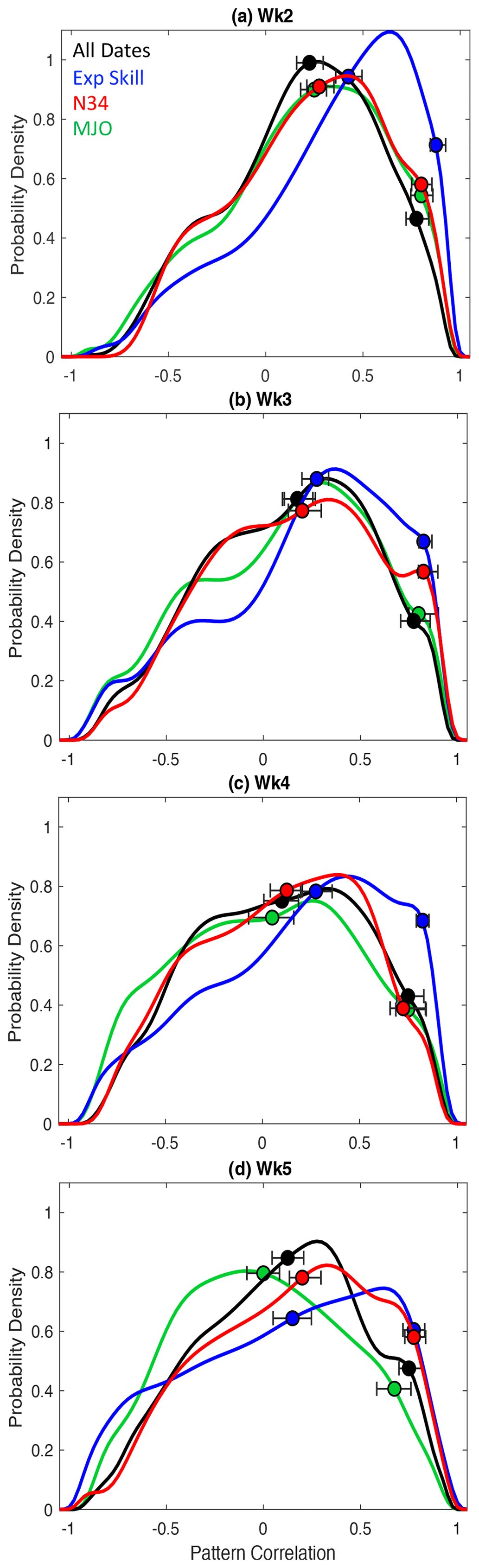
Figure 5 PDFs of the precipitation PCC for all forecasts (black lines) and the 20 % of forecasts with the highest-expected-skill (blue), the highest-Niño3.4 (red), and the highest-RMM (green) initializations. The bootstrapped confidence intervals for the median and 95th percentile of the distribution are shown with the markers.

Relating SFOs to Niño3.4 and RMM indices

The advantage of using high expected skill to anticipate SFOs is that it measures when the combined signal of all forcings (e.g., ENSO, MJO) is high relative to unpredictable noise. High expected skill occurs during periods of constructive interference between signals, while low expected skill reflects periods of deconstructive interference (e.g., Farrell, 1988; Farrell and Ioannou, 1996; Albers and Newman, 2019), and such interference is more intermittent than the individual forcing elements (Figs. 6, 8). As such, despite what is shown in Figs. 2–4, many high-expected-skill dates occur during strong ENSO and MJO events, as indicated by the overlay of SFOs (black dots) with time series of Niño3.4 (Fig. 6) and RMM (Fig. 8). The bottom 20 % of expected-skill forecasts are also shown by the vertical light gray lines to contrast the higher-frequency expected skill with the lower-frequency Niño3.4 and RMM. The correspondence to Niño3.4 is considered first. Both El Niño events of 1983 and 2016 coincided with high-expected-skill dates at weeks 3–4 and 5–6, though on different dates; conversely, the 1998 event was not associated with any high-expected-skill dates at weeks 5–6 but was for weeks 3–4. Strong La Niña events, such as in 1999, also reflect periods of high expected skill. Still, there are many high-expected-skill forecasts initialized on dates with weak Niño3.4 values, as in 2017, since other processes – including ENSO-related heating not captured by Niño3.4 – can produce a high signal-to-noise ratio. Moreover, some of the lowest-expected-skill dates occur during strong ENSO events, such as in 2016 for weeks 3–4 at the beginning of February, suggesting other processes may have been destructively interfering with the ENSO-related component.

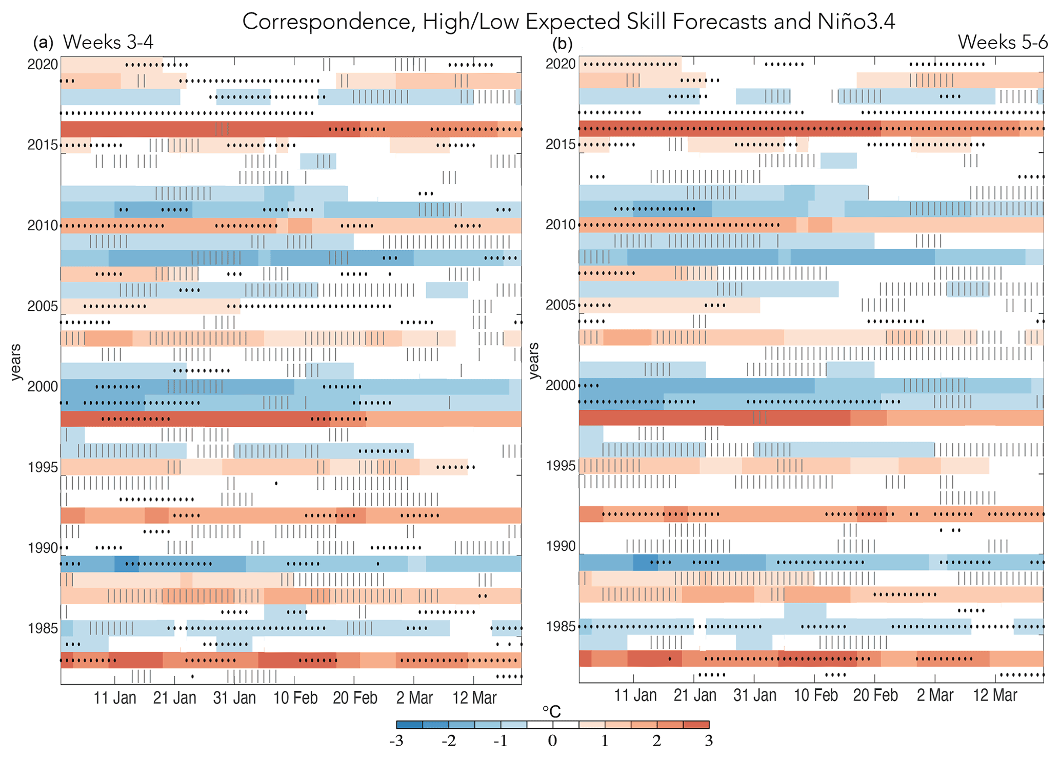
Figure 6 The color shading shows the Niño3.4 index and is the same in both panels. The black dots indicate the top 20 % of expected-skill forecasts, and the gray vertical lines represent the bottom 20 % of expected-skill forecasts, for weeks 3–4 forecasts (a) and weeks 5–6 forecasts (b).

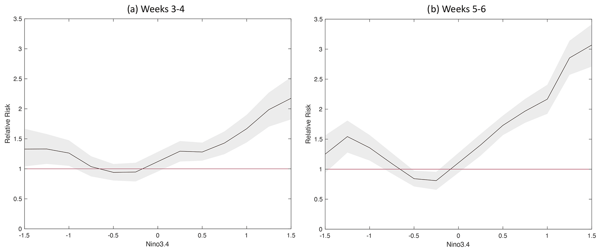
Figure 7 The black line shows the relative risk, relative to the risk on any given day, of an SFO, meaning one of the top 20 % of expected-skill dates, occurring when the Niño3.4 index is greater than various thresholds, with 95 % confidence intervals in gray shading.

High Niño3.4 index amplitude during both El Niño and La Niña events leads to increases in the risk of SFO occurrence, though more strongly during the former than the latter (Fig. 7). There is a greater relative risk for SFOs in weeks 5–6 than weeks 3–4, suggesting that at longer lead times within the subseasonal forecast period, ENSO conditions are increasingly important for SFOs. However, it is important to note that skill during these periods is overall lower than for weeks 3–4 (Figs. 3–4), which could be due to the limited capability of ENSO alone to impact predictability and/or to elevated noise. The asymmetric relative risk during El Niño and La Niña conditions may reflect the fact that there are more frequent high-amplitude El Niño events than La Niña events, increasing the number of samples at higher Niño3.4 thresholds. Indeed, Niño3.4 exceeds 1.5 ^∘C on 269 d, compared to 192 d where Niño3.4 is less than −1.5 ^∘C. The stronger response during El Niño conditions than La Niña could also be consistent with Hoell et al. (2018a), who found precipitation shifts during both CP and EP El Niño events but only CP La Niña events, although future work is needed to better explore these nuances.

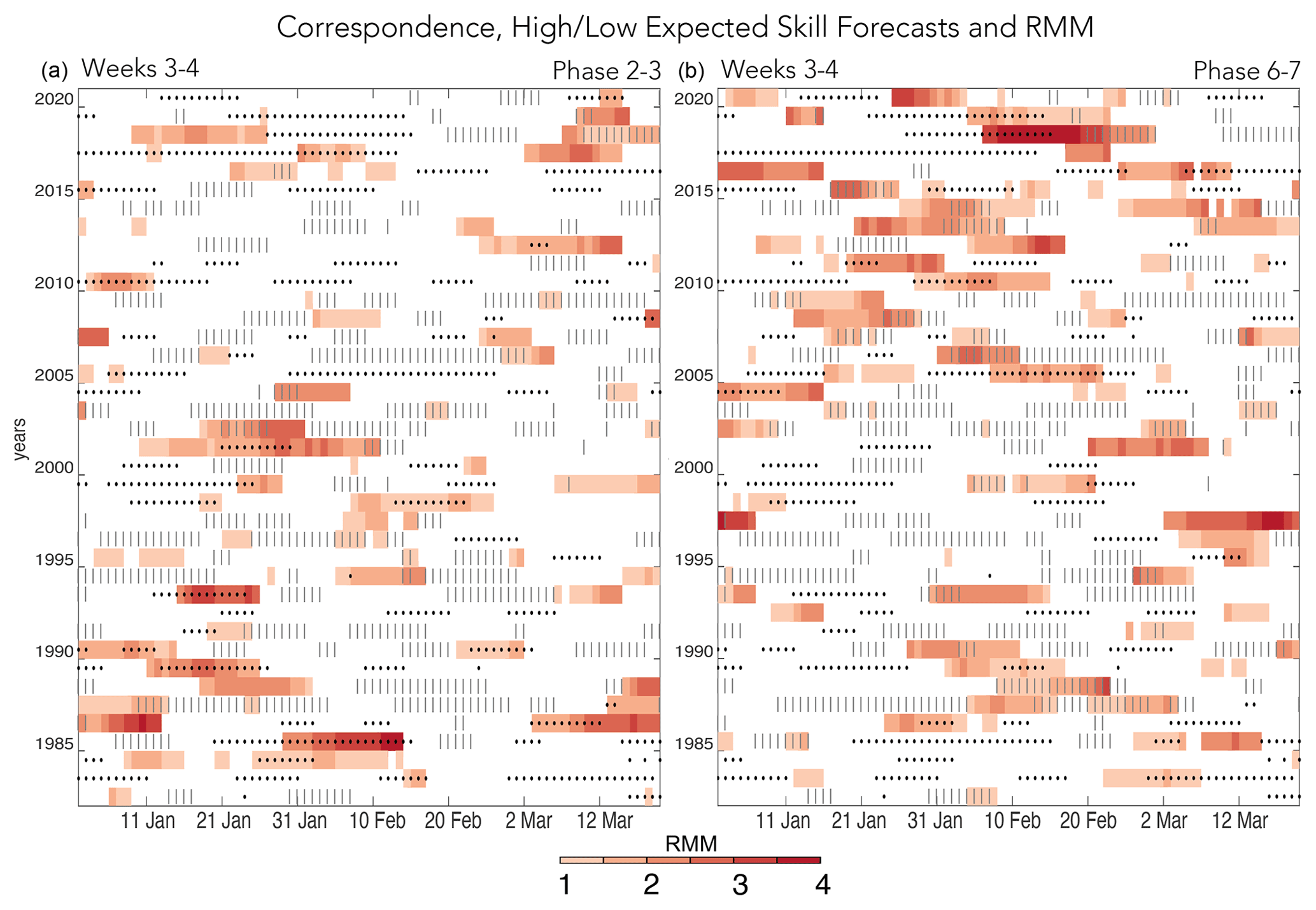
Figure 8 As in Fig. 6 but for the amplitude of the RMM index during (a) MJO phases 2–3 and (b) MJO phases 6–7 and for weeks 3–4 expected-skill dates.

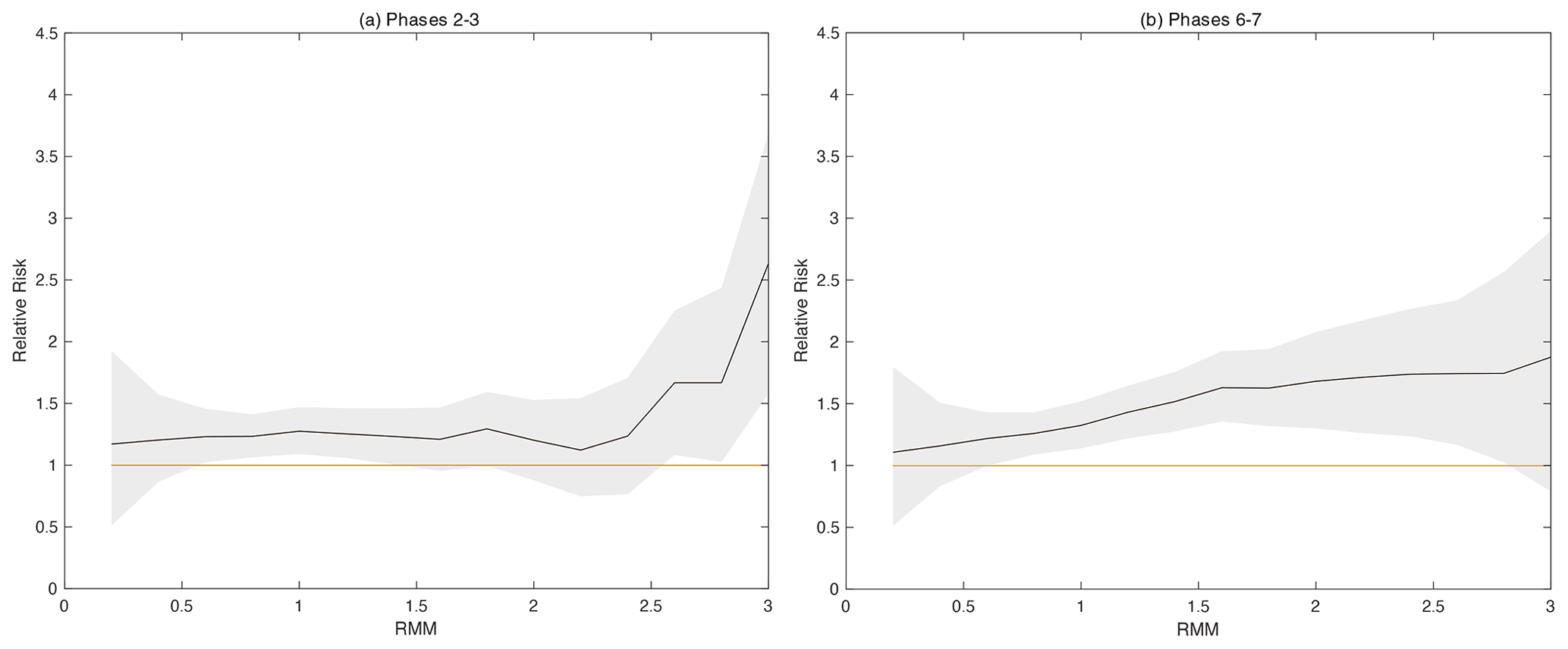
Figure 9 As in Fig. 7 but for weeks 3–4 expected skill and for varying RMM amplitude during either (a) MJO phases 2–3 or (b) MJO phases 6–7.

Discerning a relationship between MJO phases 2–3 and 6–7, the phases that impart known teleconnections to southwest Asian precipitation (Hoell et al., 2018b), can be more difficult given the more transient nature of the MJO compounded with transient expected skill (Fig. 8). Only the relationship between RMM and weeks 3–4 expected skill is considered, as an MJO teleconnection at 5–6-week lead times is not physically plausible (e.g., Tseng et al., 2018). Still, we do find that particularly strong events for phases 2–3 and 6–7 increase the relative risk of weeks 3–4 SFOs, though sampling introduces spread into these estimates (Fig. 9). Some particularly high-amplitude MJO events, including phases 2–3 in 1985 and 1993 and phases 6–7 in 2005 and 2018, overlap with periods of weeks 3–4 high expected skill, while some weaker-amplitude events overlap with some of the lowest-expected-skill dates, such as phases 2–3 in late January 2002. The strong RMM phases 6–7 are also associated with an increase in the relative risk of SFOs, which increases at lower RMM thresholds compared to in phases 2–3 and does not display the exponential increase at the highest thresholds. These subtle differences in relative-risk sensitivity could reflect true differences in the MJO teleconnection to the region or could be due to sampling, as there is high uncertainty in the relative-risk estimates given the small number of events observed at such high thresholds.

3.2 Characteristics of predictable dry and wet initializations

This section considers the composite patterns preceding predictable wet and dry periods 18 d earlier, revealing the role of anomalous heating near the SPCZ. Next, composite wet and dry periods are split by their Niño3.4 sign, revealing how different circulation responses during each phase produce same-signed precipitation anomalies over southwest Asia.

3.2.1 All initializations

First, we consider the patterns preceding anomalously wet and dry periods regardless of ENSO phase, where “wet” and “dry” are defined using the top and bottom terciles of southwest Asian precipitation anomalies, respectively. Wet and dry dates that were associated with weeks 3–4 high-expected-skill dates initialized 18 d earlier and were also characterized by a PCC > 0 are considered. A lead time of 18 d is chosen because it falls within the weeks 3–4 forecast period and provides the clearest circulation structures, which are similar but weaker at longer lead times (not shown). An 18 d lag is also consistent with the circulation response to tropical diabatic heating anomalies discussed in Jin and Hoskins (1995), which peaked about 15 d after the heating occurred. For these skillful, high-expected-skill forecasts associated with the development of anomalously wet or dry precipitation anomalies, we consider the composite circulation and heating patterns observed at the time of initialization, meaning 18 d before the anomalous precipitation was observed.

Figure 10 shows that during weeks 3–4 SFOs initialized before predictable wet and dry periods over southwest Asia, anomalies are roughly equal and opposite in sign. Before dry periods, positive OLR anomalies are located over the western and central tropical Pacific, signifying suppressed convection, while a 200 hPa anticyclone (positive Ψ₂₀₀ anomaly) is located over southwest Asia, consistent with downward vertical motion and suppressed precipitation. Conversely, predictable anomalously wet periods are associated with enhanced anomalous central Pacific convection and a cyclonic Ψ₂₀₀ anomaly over southwest Asia. One feature present during dry initializations is a small but statistically significant negative OLR anomaly in the eastern Indian Ocean, which does not have a counterpart during wet initializations. Southwest Asian precipitation is strongly linked to heating variability in this location (Hoell et al., 2012), and the results here suggest that the relationship might be particularly important for anomalously dry periods.

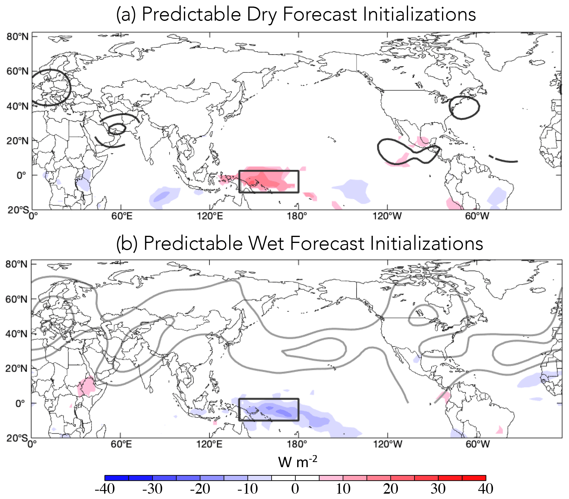
Figure 10 Composite OLR (color shading) and Ψ₂₀₀ (black/gray contours) anomalies, during (a) high-expected-skill initializations verified on anomalously dry days 18 d later, N = 142 d, and (b) high-expected-skill initializations verified on anomalously wet days 18 d later, N = 163. The black contours show positive (anticyclonic) streamfunction anomalies, and the gray contours show negative (cyclonic) streamfunction anomalies, contoured at an interval of 3 × 10⁶ m² s⁻¹ beginning at ±3 × 10⁶ m² s⁻¹. Only anomalies that are statistically significant at the 95 % confidence level are shown.

3.2.2 El Niño and La Niña initializations

Section 3.1 indicated that, while anticipating SFOs based on the Niño3.4 index alone is less successful than expected skill (Figs. 3–4), periods of strong ENSO activity increase the likelihood of a forecast of opportunity occurring, particularly during the strongest events (Fig. 7). During either ENSO phase, periods of anomalously high and low precipitation can occur due to transient disturbances forming along the subtropical jet. However, the manner in which precipitation anomalies develop differs between El Niño and La Niña, due to ENSO's influence on the mean jet and baroclinic waves (Shapiro et al., 2001), whose life cycles differ under different mean states (Thorncroft et al., 1993). This section examines how predictable wet and dry initializations differ by ENSO phase given the hypothesized differences in teleconnections in each phase.

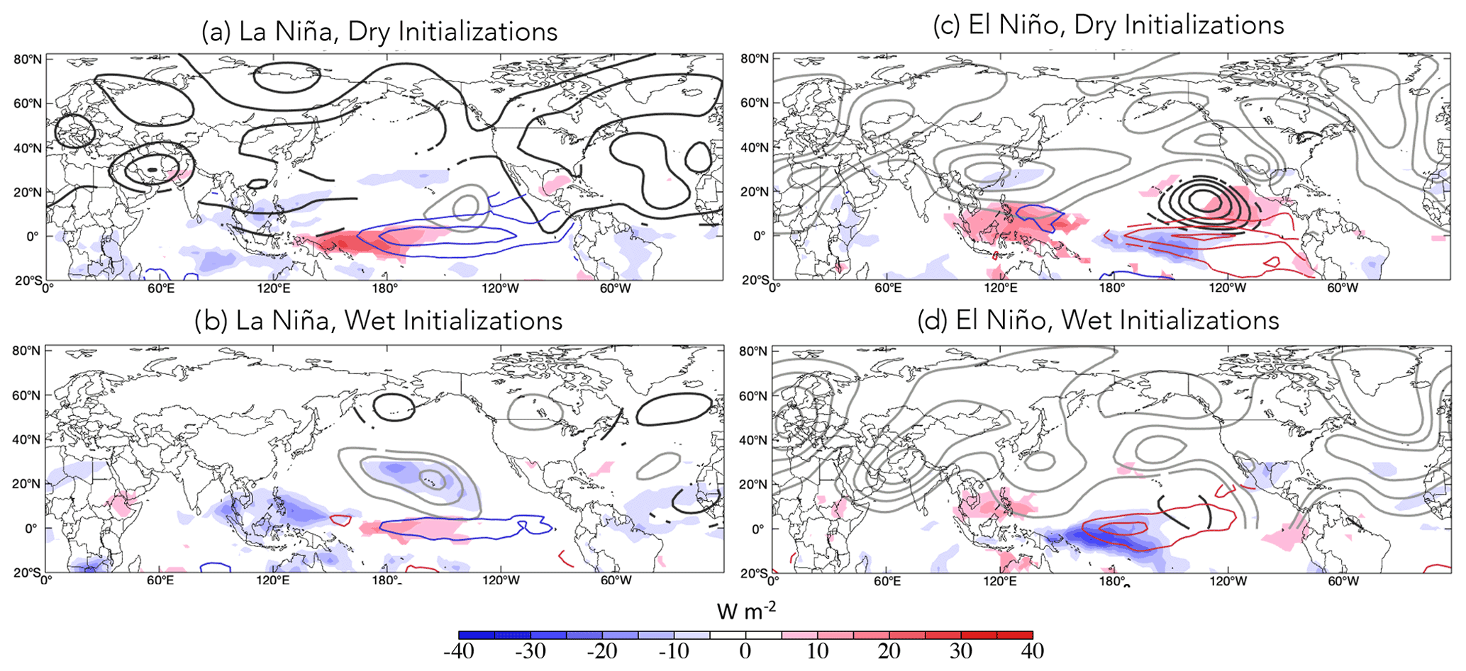
Figure 11 As in Fig. 10 but for groups divided by Niño3.4 < 0 (“La Niña”) or Niño3.4 > 0 (“El Niño”) and with negative SST anomalies in blue contours and positive SST anomalies shown in red, at a contour interval of 0.5 ^∘C.

Splitting dry and wet forecast initializations into periods when Niño3.4 is positive or negative to reflect El Niño or La Niña conditions, without losing any samples, indicates that even when preceding same-signed precipitation anomalies, El Niño and La Niña conditions are associated with different large-scale circulation patterns (cf. Fig. 11a, c and b, d). By construction, there are clear differences in SST and OLR associated with El Niño and La Niña conditions, as well as North Pacific Ψ₂₀₀ anomalies associated with ENSO-like tropical heating (Winkler et al., 2001; Breeden et al., 2020; Henderson et al., 2020). During La Niña conditions, dry periods include an anticyclonic anomaly over southwest Asia, while during dry El Niño initializations there are cyclonic features north and east of southwest Asia and weak anomalies directly over the region (cf. Fig. 11a, c). In contrast to the circulation pattern during dry El Niño periods (Fig. 11c), during wet periods, El Niño conditions are associated with an amplified Ψ₂₀₀ pattern, with two high-amplitude cyclonic anomalies located over Eurasia (Fig. 11d). Conversely, at the time of initialization during wet La Niña periods, negligible Ψ₂₀₀ anomalies are observed (Fig. 11b).

What distinguishes rainy La Niña or El Niño periods from dry La Niña or El Niño periods? While the heating and SST dipole patterns are consistent with each ENSO phase for both wet and dry periods, there are differences in heating strength and location (cf. Fig. 11a, b and c, d). Dry La Niña initializations include stronger negative SST anomalies and suppressed convection in the central Pacific compared to rainy periods, which instead involve enhanced convection over the Maritime Continent. Dry El Niño periods include stronger suppressed convection over the Maritime Continent than wet El Niño dates, coinciding with a hint of a wave train emanating from the eastern Pacific across North America and the North Atlantic. Dry La Niña dates are more common than wet La Niña dates, 84 vs. 67 d, while wet El Niño dates are more common than dry El Niño dates, 96 vs. 57 d, which is consistent with past research linking seasonal mean departures of southwest Asian precipitation to ENSO (Hoell et al., 2018a).

Differencing the dry and wet composites between each ENSO phase reveals the common element of suppressed SPCZ convection and cooler central Pacific SSTs during dry periods relative to wet periods (Fig. 12). Dry periods during El Niño conditions are associated with warmer SSTs in the eastern Pacific than are wet periods (Fig. 12b), while no such differences in SSTs or OLR are observed in the eastern Pacific during La Niña conditions (Fig. 12a). While distinct from one another, the Ψ₂₀₀ patterns during both El Niño and La Niña conditions place an anomalous anticyclone over southwest Asia during dry events, consistent with suppressed precipitation. The Ψ₂₀₀ patterns during dry versus wet periods differ, with La Niña conditions displaying weak anticyclonic anomalies in the subtropical North Pacific and North Atlantic and El Niño conditions associated with an upper-level wave train emanating from the eastern tropical Pacific, across the North Atlantic to Europe, potentially linked to the anomaly over southwest Asia. The orientation of such a wave train is consistent with the evolution described by Shaman and Tziperman (2005), who found a northeastward-propagating wave train emanating from the eastern central Pacific during strong ENSO events, which ultimately modulated Tibetan snow depth. Thus, while the heating difference between dry and rainy periods is similar regardless of the ENSO phase, the impact of the anomalous heating on the circulation is different but coincidentally yields a reduction in precipitation over southwest Asia. The different circulation responses are consistent with the modified mean states of each ENSO phase, though more work is required to further understand these nuanced relationships, preferably with a larger sample size. Dry baroclinic modeling experiments could be useful in disentangling the role of the basic state and thermal forcing in producing this response.

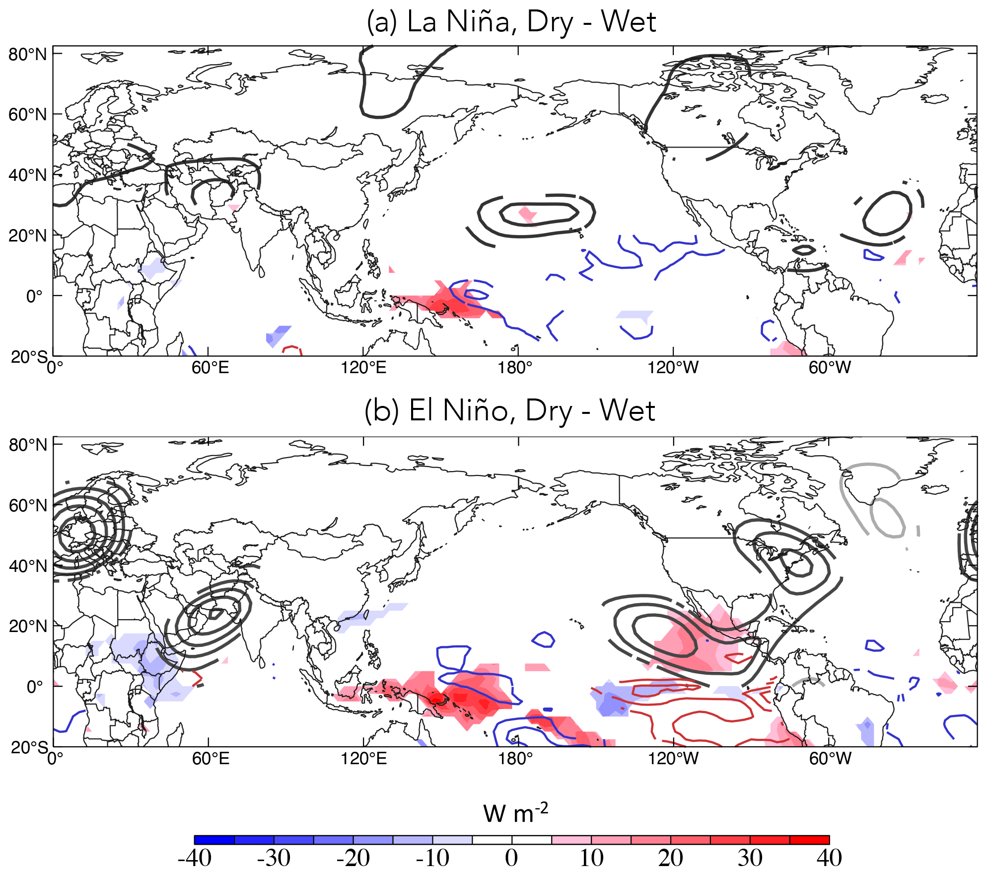
Figure 12 Composite difference, dry − wet, during (a) La Niña conditions (Fig. 11a–b) and (b) El Niño conditions (Fig. 11c–d). Plotting conventions are as in Fig. 11, except the contour interval for SST anomalies (blue and red contours) is 0.25 ^∘C.

3.2.3 Relative risk associated with SPCZ OLR

Given the OLR anomalies in the SPCZ region noted during both predictable wet and predictable dry forecast initializations (Figs. 10, 12), a time series of OLR over the region was selected for a final metric to consider related to weeks 3–4 SFOs. Similarly to considering Niño3.4 and RMM, the relative risk of an SFO occurring increases significantly as the standard deviation of SPCZ OLR anomalies increases (Fig. 13). The response during negative and positive SPCZ OLR anomaly values is more symmetric than the risk associated with an increasing Niño3.4 threshold, which indicated a greater relative-risk increase during El Niño than during La Niña conditions (Fig. 7), or comparing the impact of MJO phases 2–3 vs. 6–7 (Fig. 9). This symmetry is further supported with the 18 d lagged regression of the southwest Asian precipitation time series with OLR (Fig. S2), although the regression pattern OLR anomalies are weaker than the composite OLR during the SFOs considered in Figs. 10 and 12. The SPCZ OLR time series is correlated with the Niño3.4 index at r = −0.25, an indication that the SFOs associated with SPCZ OLR are not redundant with Niño3.4-related SFOs and therefore contain additional information about SFOs related to tropical variability. As such, the expected-skill approach to SFOs benefits from measuring shifts in the likelihood of a forecast of opportunity captured by several distinct indices tracking tropical variability, Niño3.4, RMM, and SPCZ OLR, a distinct advantage over using an index that tracks only one of these processes (Figs. 3–4).

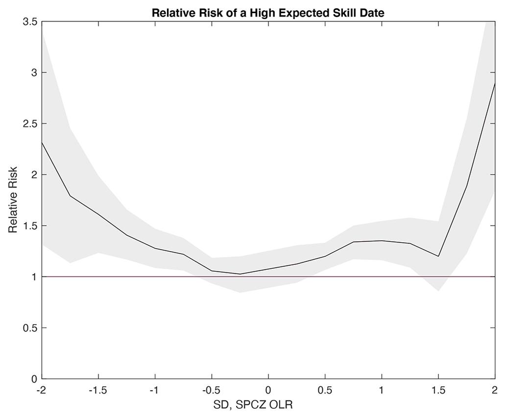
Figure 13 As in Fig. 7 but for using the standard deviation of the SPCZ OLR anomaly time series, calculated using the boxed region in Fig. 10 and for weeks 3–4 expected skill.

4 Conclusions

In this study, precipitation SFOs are considered over southwest Asia using LIM expected skill, a metric related to the forecast signal-to-noise ratio that leverages the constructive interference of all signals impacting predictability. Strong El Niño, La Niña, and MJO phase 2–3 and phase 6–7 conditions increase the chances that an SFO occurs. A third tropical heating index, based on anomalous OLR in the SPCZ region, also increases the risk of an SFO (Fig. 13). The correspondence between expected skill and several indices highlights the advantage of using expected skill, in that all of these flavors of tropical heating are registered as high signals. However, there are still SFOs that do not correspond to any one of these indices, since other processes, potentially not tropically driven, can produce a high signal too. Future work could focus on categorizing all SFOs to examine these potential additional factors.

In addition to the confirmed influence of ENSO and MJO activity on southwest Asian precipitation, anomalous heating across the SPCZ region is a common element among predictable wet and dry initializations and increases the relative risk of an SFO. Heating in this region is also associated with different circulation patterns during El Niño and La Niña conditions (Fig. 12). How these different circulation patterns are related to similarly located anomalous heating anomalies is currently not well understood but likely involves the modified tropopause-level waveguide present during each ENSO phase, which modulates the extratropical response to tropical heating (Sardeshmukh and Hoskins, 1988; Newman and Sardeshmukh, 1998; Shapiro et al., 2001). Dry baroclinic modeling experiments with idealized heating could be used to quantify the contribution of tropical heating over the Indian Ocean and western Pacific affecting the circulation over southwest Asia on subseasonal timescales. We also note that, while widely used, ENSO indices such as Niño3 or Niño3.4 do not capture the full spectrum of ENSO variability (Penland and Sardeshmukh, 1995; Newman et al., 2009; Gehne et al., 2014; Henderson et al., 2020; Albers and Newman, 2021). Future work could employ the dynamical decoupling approach of Henderson et al. (2020) to isolate the ENSO signal and its impact on precipitation SFOs more holistically.

The association between forecasts of opportunity and the MJO is less constrained given the higher-frequency nature of the MJO and small sample size once RMM is sorted by phase, but it still indicates a role for strong MJO events in phases 2–3 or 6–7 to increase the likelihood of a weeks 3–4 SFO occurring, consistent with prior studies (Cannon et al., 2017; Hoell et al., 2018b). Further suggesting a role for MJO-like heating, predictable heating patterns associated with forecasts of opportunity indicate a role for anomalous convection over the Indian Ocean during dry periods, consistent with MJO phases 2–3 suppressing southwest Asian precipitation (Fig. 10a). Future work could employ large climate simulation output to enhance sample size and revisit the MJO–expected-skill relationship and the extent the model can reproduce the mean state and the MJO itself. Another remaining question that could be addressed more aptly with a larger sample size is how ENSO and the MJO act together to impact SFOs for southwest Asian precipitation events, particularly concerning their magnitude and duration, which was beyond the scope of this study but merits further investigation.