the Creative Commons Attribution 4.0 License.
the Creative Commons Attribution 4.0 License.
 | 22 Dec 2022
European heatwaves in present and future climate simulations: a Lagrangian analysis
Lisa Schielicke
Stephan Pfahl
Heatwaves are prolonged periods of anomalously high temperatures that can have devastating impacts on the environment, society and economy. In recent history, heatwaves have become more intense and more numerous over most continental areas, and it is expected that this trend will continue due to the ongoing global temperature rise. This general intensification may be modified by changes also in the underlying thermodynamical and dynamical processes. In order to study potential changes in heatwave characteristics and dynamics, we compare Lagrangian backward trajectories of airstreams associated with historic (1991–2000) and future (2091–2100) heatwaves in six different European regions. We use a percentile-based method (Heat Wave Magnitude Index daily) to identify heatwaves in a large ensemble of climate simulations (Community Earth System Model Large Ensemble (CESM-LE) with 35 members). The simulations have been forced by historical representative concentration pathways (RCPs) up to 2005 and by the RCP8.5 scenario afterwards. In general, we find that air parcels associated with heatwaves are located to the east or inside the respective regions 3 d prior to the events. For future heatwaves, the model projects a north-/northeastward shift of the origin of the air masses in most study regions. Compared to climatological values, airstreams associated with heatwaves show a larger temperature increase along their trajectory, which is connected to stronger descent and/or stronger diabatic heating when the air parcels enter the boundary layer. We find stronger descent associated with adiabatic warming in the northern, more continental regions and increased diabatic heating in all regions (except of the British Isles) in the simulated future climate. The enhanced diabatic heating is even more pronounced for heatwaves over continental regions. Diabatic temperature changes of near-surface air are driven by sensible heat fluxes, which are stronger over dry soils. The amplified diabatic heating associated with future heatwaves may thus be explained by an additional drying of the land surface.
- Article
(16582 KB) - Full-text XML
-
Supplement
(17826 KB) - BibTeX
- EndNote


Heatwaves can have huge socioeconomic impacts including an increased mortality (Guo et al., 2017), an enhanced risk of wildfires due to hot and dry conditions accompanying heatwaves (Jones et al., 2020), crop failures in connection with droughts (Zampieri et al., 2017), and damage to the flora in general (Breshears et al., 2021). Impacts to the water, transport and energy infrastructures can lead to tremendous economic losses that are expected to increase in the future (see Forzieri et al., 2018, who studied these impacts for Europe). In their Sixth Assessment Report, the Intergovernmental Panel on Climate Change (IPCC) states that “hot extremes (including heatwaves) have become more frequent and more intense across most land regions since the 1950s” (IPCC, 2021). Due to the expected ongoing rise in the global mean temperature in the 21st century, this progress is expected to continue (Meehl and Tebaldi, 2004). It is therefore of general interest to study the differences between historic and future heatwaves. Understanding changes in their dynamics, variability and underlying processes can further help to quantify future changes in heatwave occurrence and to take measures to protect against their impacts.
In general, heatwaves are long periods of unusually high temperatures (Perkins and Alexander, 2013). However, there is no common, global heatwave definition, and thresholds differ from region to region due to locally different climates. Heatwave identification can be based on absolute or relative thresholds of a certain temperature measure, for example, the daily maximum or minimum temperature (see, e.g., Perkins and Alexander, 2013; Perkins, 2015, for a discussion of different heatwave definitions). Absolute thresholds are fixed and therefore do not account for a general increase in mean temperatures. Hence, an increase in global mean temperature will naturally lead to a higher number of identified heatwave events if these thresholds are not adjusted to the new climate. Indeed, Vogel et al. (2020) observe an increase in heatwaves for fixed temperature thresholds, but they only see relatively small changes for moving, i.e., temporally varying, thresholds. In order to investigate future changes in heatwaves beyond mean climate warming, we will take a relative, percentile-based threshold (after Russo et al., 2015) that is adapted to the respective climate. This allows for the identification and comparison of heatwaves in different (European) regions, climates and time slices with different background temperatures.
Dynamically, heatwaves are linked to quasi-stationary atmospheric blocking patterns (e.g., Pfahl and Wernli, 2012, who showed this relationship for the Northern Hemisphere) or extended ridges (Sousa et al., 2018). Such anticyclonic circulation anomalies lead to the buildup of warm temperature extremes in summer due to the associated subsidence and adiabatic warming, the clear-sky conditions that lead to surface heating by solar radiation, low wind speeds and warm-air advection (Meehl and Tebaldi, 2004; Pfahl, 2014; Bieli et al., 2015; Zschenderlein et al., 2019; Kautz et al., 2022). Moreover, soil-moisture–atmosphere feedbacks enhance the heating of lower tropospheric air in the planetary boundary layer due to the increase in sensible heat fluxes and decrease in latent heat fluxes associated with reduced soil moisture content during (prolonged) drought and heatwave conditions (Fischer et al., 2007; Seneviratne et al., 2010; Stéfanon et al., 2014; Miralles et al., 2019).
Several previous studies have shown that detailed insights into the processes leading to hot extremes and heatwaves can be obtained from a Lagrangian description of the associated air mass trajectories (Bieli et al., 2015; Santos et al., 2015; Quinting et al., 2018; Schumacher et al., 2019; Zschenderlein et al., 2019, 2020; Catalano et al., 2021). Such a Lagrangian approach allows for differentiating between thermodynamic and dynamic contributions to the warming of air masses. Investigating 10 d backward trajectories initiated close to the surface, Bieli et al. (2015) found that hot events are connected to strong adiabatic and diabatic warming but only to weak northward transport of warm air from the south towards their European study regions (British Isles, Central Europe and the Balkans region). Furthermore, Bieli et al. (2015) found that hot extremes in the regions closer to the ocean (British Isles and Balkans) are often dominated by dynamical processes, i.e., adiabatic warming due to descent, while in their continental region (Central Europe) local, diabatic heating by surface fluxes is more important. Zschenderlein et al. (2019) extended the Lagrangian investigation to six different European regions and additionally clustered the trajectories with respect to the prevailing diabatic warming or cooling and strong or weak descent occurring along the air parcel trajectories. They confirmed the finding of weak horizontal transport associated with heatwaves. Schumacher et al. (2019) used backward trajectories to show that heatwaves can be intensified due to enhanced sensible heat fluxes in upwind regions affected by drought conditions.
The above-cited Lagrangian heatwave studies focused on the analysis of past events based on reanalysis data and did not investigate potential future changes in these Lagrangian dynamics. In principle, future changes in heatwaves beyond the mean climate warming may be due to changes in the associated atmospheric dynamics (e.g., varying transport patterns or adiabatic warming) or thermodynamics (e.g., altered sensible heating near the surface). Schaller et al. (2018) and Brunner et al. (2018) showed that the link between atmospheric blocking and European heatwaves appears to be relatively stable in ensemble simulations of future climate, suggesting that dynamical changes might be of minor importance. Also Vogel et al. (2020) concluded that future changes in heatwaves are mainly driven by thermodynamic processes and changes in the underlying atmospheric dynamics are small. Rasmijn et al. (2018) hypothesize a disproportional intensification of future (continental) heatwaves in Western Russia due to amplified sensible heating linked to soil moisture feedbacks.
In this study, a detailed Lagrangian analysis of future changes in the processes associated with European heatwaves is presented. In particular, we investigate the following research questions:
-
How will the atmospheric transport patterns associated with European heatwaves change in a warming climate?
-
Will changes in thermodynamic or dynamic processes lead to an amplification of heatwaves beyond mean warming?
Since heatwaves are rare events, we use an ensemble data set of climate simulations with 35 members to increase the number of heatwave events in a historic (1991–2000) and a future (2091–2100) time slice. The data and methods including the definition of the regions and the identification of heatwaves are described in Sect. 2. The results are presented and discussed in Sect. 3, followed by a summarizing discussion and conclusion in Sect. 4.
In this section, we give an overview of the data used (Sect. 2.1) and define the six European study regions (Sect. 2.2). The heatwave identification follows the work of Russo et al. (2015) adapted to the ensemble data and is described in Sect. 2.3. Finally, the trajectory calculations and clustering using the Lagrangian tool LAGRANTO (Sprenger and Wernli, 2015) are described in Sect. 2.4.
2.1 CESM-LE data
In this study, we use data from model simulations based on the Community Earth System Model (CESM) Large Ensemble (CESM-LE) project (Kay et al., 2015) with 35 ensemble members. The ensemble members have been generated through small differences in their initial conditions – mainly by adding random perturbations on the order of 10−14 K to the initial air temperature fields. The simulations have been externally forced by the historical (up to the year to 2005) and representative concentration pathway (RCP) 8.5 (years 2006 to 2100) conditions. The atmospheric variables of the CESM-LE data have a horizontal grid spacing of approximately ≈1∘ in latitudinal and 1.25∘ in longitudinal direction and 30 hybrid vertical levels. Reruns of the simulations have been performed for two 10-year time slices, 1991–2000 (historic) and 2091–2100 (future), based on restart files from the original CESM-LE simulations and using the exact same model setup, in order to obtain additional output fields (in particular of 6-hourly vertical wind on model levels) required for the trajectory calculations. The identification of the heatwaves is based on the temperature at reference height (2 m above ground). Furthermore, we use 6-hourly three-dimensional wind fields as well as pressure, potential temperature, and air temperature to study heatwave properties and calculate parcel trajectories with LAGRANTO (see Sect. 2.4 for more details).
It is a limitation of this study that it is based on one climate model only. Nevertheless, previous studies have shown that the CESM-LE simulations compare reasonably well to observational data and other models in the representation of temperature trends (Kay et al., 2015), the frequency of atmospheric blocking (Kay et al., 2015), and the relationship between European heatwaves and blocking (Schaller et al., 2018), which shows that the model is well suited for our analysis of heatwave-related circulation changes.
2.2 Definition of study regions
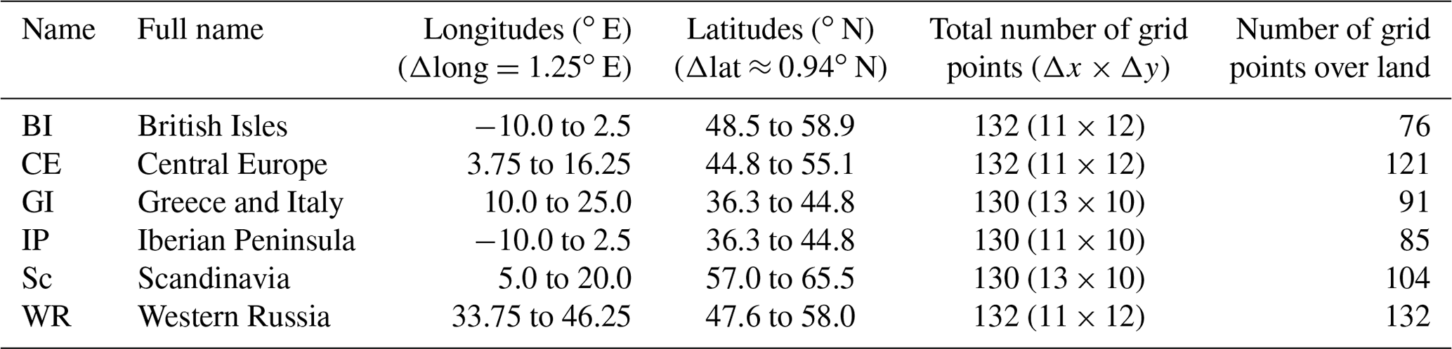
We study heatwaves in historic and future time slices in six European regions with different climates: the British Isles (BI), Central Europe (CE), Greece and Italy (GI), the Iberian Peninsula (IP), Scandinavia (Sc), and Western Russia (WR). Thereby, we follow the definitions of the regions by Zschenderlein et al. (2019). Details on the six regions with respect to the CESM-LE data are summarized in Table 1. The study regions are marked in Fig. 1.
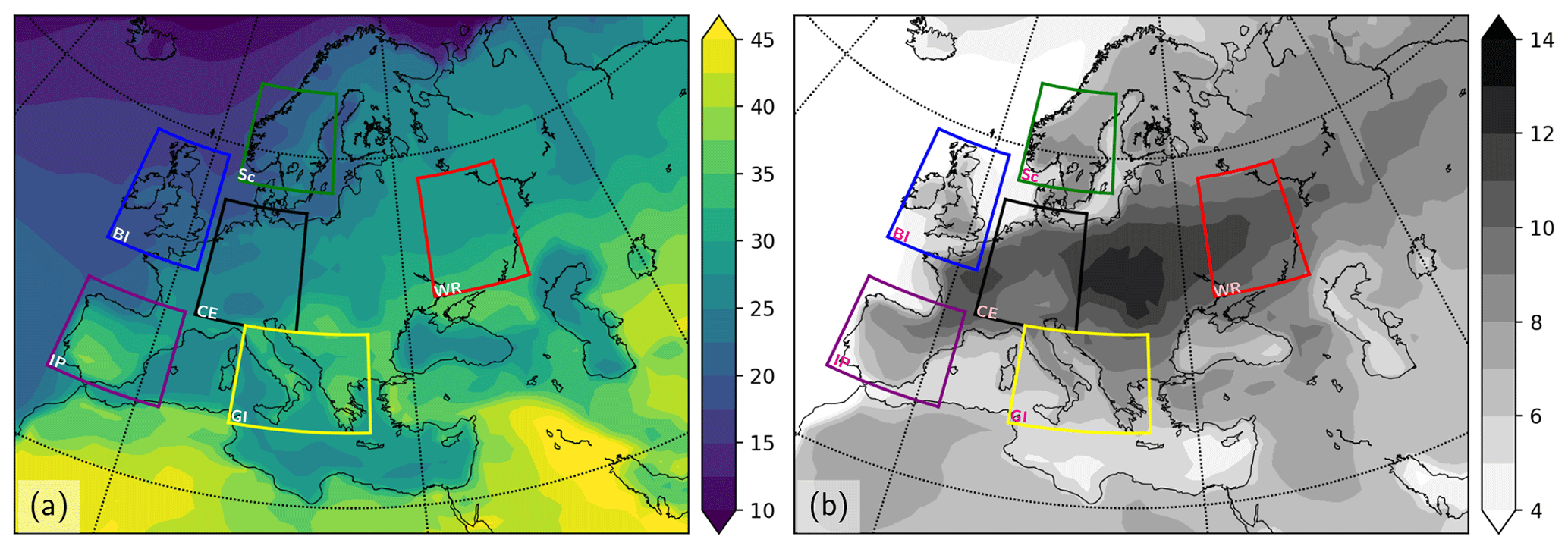
Figure 1The 90th percentile of daily maximum 2 m temperature in August: (a) historic time slice (1991–2000), in degrees Celsius; (b) difference (in K) between future (2091–2100) and historic time slices. Shown is the 90th percentile centered on 15 August, which is derived by taking into account all daily maximum temperatures from 1–31 August (15 August ± 15 d) in the respective time slice. Colored boxes show the outline of the different European regions (see Table 1).
Table 1Definition of regions representing different European climates (following Zschenderlein et al., 2019, with adaptions to the CESM-LE data). Latitudes are rounded.
2.3 Identification of heatwaves
A heatwave is defined if a specific temperature threshold at a grid point is exceeded for at least 3 consecutive days in a large area. In our analysis, this temperature threshold is given by the 90th percentile of the daily maximum temperature (calculated as the maximum over four 6-hourly time steps) within a 30 d window around the day of interest. The 90th percentile is derived by taking into account all years in the historic or in the future time slice simulations, respectively. For example, for the calculation of the daily maximum temperature percentiles of 15 August, the 30 d period around the date, i.e., the period of 1 to 31 August, in all 350 years (35 members times 10 years per time slice) is considered (see Fig. 1). Accordingly, heatwaves are defined with respect to the historic climate (percentiles calculated form the historic period) in the 1991–2000 time slice and with respect to future climate in the 2091–2100 time slice.
In order to estimate the magnitude of a heatwave, the percentile-based Heat Wave Magnitude Index daily (HWMId) is used, as defined by Russo et al. (2015). It is based on the calculation of the daily heatwave magnitude Md, which is given as
with daily maximum temperature Td,max and the 25th (75th) percentile of annual maximum temperature TΔy,25th (TΔy,75th) that occurred within a time range of Δy years (e.g., Δy=30 years in Russo et al., 2015). In our case, the time range Δy is given by each 10-year time slice considering all 35 ensemble members, i.e., Δy=350 years for the historic and the future run, respectively. The annual maximum temperature at a grid point represents just one value per year, i.e., the maximum of the 2 m temperature observed in this year. Percentiles TΔy,25th and TΔy,75th are then calculated from the 350 values in each time slice (35 members times 10 years). Since the annual maximum temperature typically occurs in the warm season, Md>0 is connected to the warmer season. We decided to use different climatologies for the two time slices since, otherwise, the method would mainly detect heatwaves in the future time slice due to the mean increase in global temperature in the future (see Fig. 2). As can be seen in Fig. 2, heatwaves in the historic times slice have mean temperatures comparable to the future mean summer (June–July–August) temperatures. Since the focus of this work is on a comparison of historic and future heatwave characteristics, the heatwave identification needs to be done for each time slice separately. The Md values are calculated at each grid point, and summing them up gives the HWMId per day in a specific region. In order to account for the large-scale character of heatwaves, we additionally use a minimum area criterion of at least 5 % of all grid points over land that must satisfy Md>0. The latter criterion (Md>0) also makes sure that heatwaves occur during the warmest time of the year, typically the summer months. Note that we detect more heatwave days towards the end of the two time slices due to the general temperature increase during the 10-year periods.
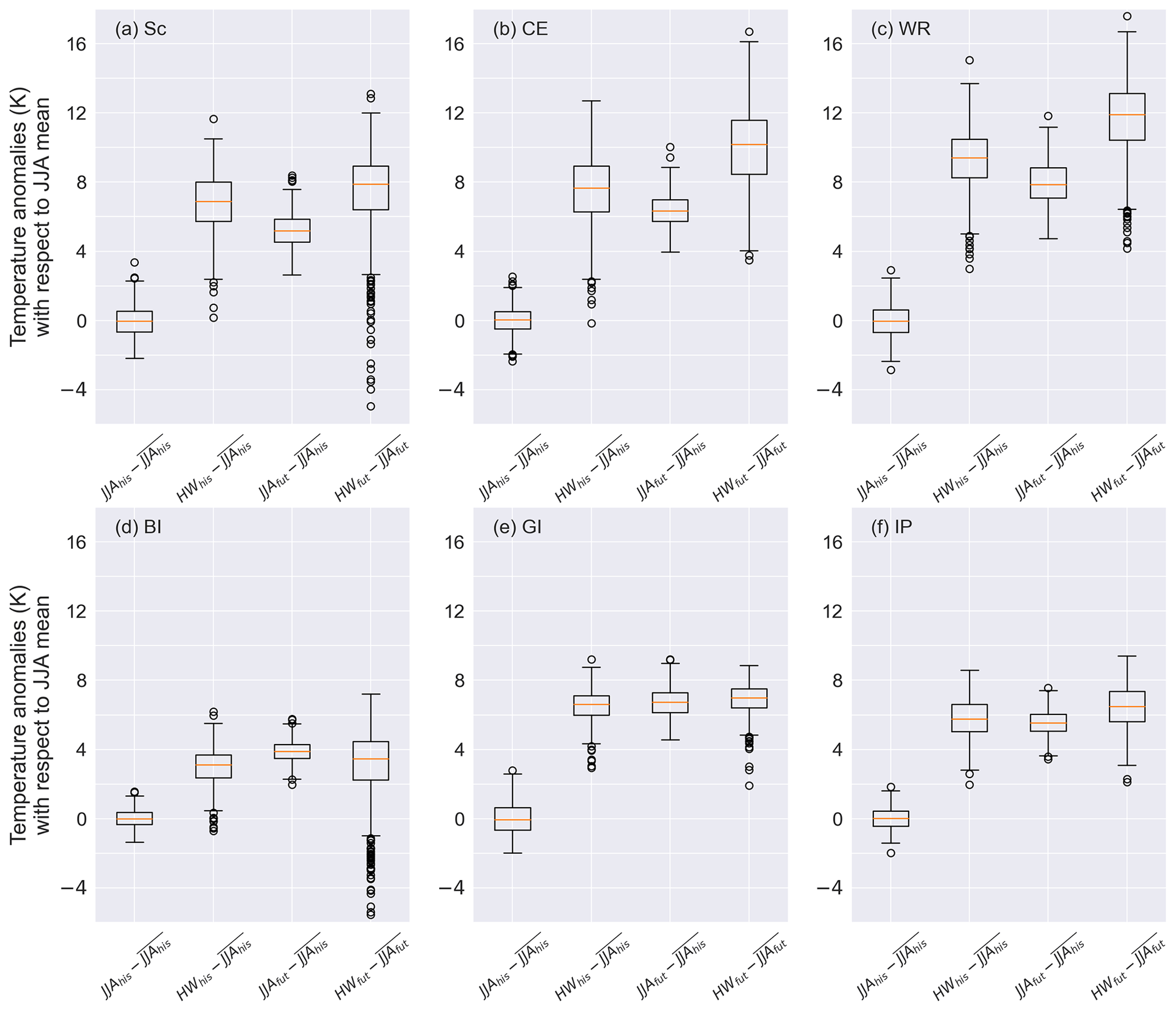
Figure 2Temperature anomalies at 12:00 UTC (in Kelvin) with respect to the JJA mean temperature per time slice (, ) in the regions (a) Sc, (b) CE, (c) WR, (d) BI, (e) GI and (f) IP. JJA mean temperatures are calculated over each year of the time slice (historic: 1991–2000; future: 2091–2100) and each ensemble member. The heatwave temperatures are determined as spatial average temperature per region for each heatwave day. Note that no differentiation between grid points over land/ocean are made here. For the first three boxes from the left, temperature anomalies are calculated by subtracting the JJA mean temperature of the historic time slice. The second (fourth) box shows the historic (future) heatwave (HW) temperature HWhis (HWfut) anomalies with respect to the JJA mean temperature () of the (historic) future time slice. The box spans the 25th and 75th percentile of the data, the horizontal (orange) line inside the box gives the median, and the whiskers are given by 1.5 times the interquartile range; flier points are those that are outside the range of the whiskers.
2.4 Trajectory calculation and clustering
LAGRANTO (Sprenger and Wernli, 2015) is a Lagrangian analysis tool that allows the calculation of backward and forward trajectories based on various data sets. LAGRANTO can be used to interpolate other variables of interest such as temperature or potential temperature along the trajectory paths and thus study physical processes, such as diabatic and adiabatic heating, in three-dimensional airstreams. In this work, we use LAGRANTO to calculate 10 d backward trajectories. These air parcels are started 10, 30, 50 and 100 hPa above the surface at land grid points that satisfy the heatwave criterion. The trajectories are started at 12:00 UTC on each heatwave day in the respective region. In order to compare the heatwave trajectories with typical climatological values, we additionally start 10 d backward trajectories at 12:00 UTC on each day in the boreal summer period (JJA: June, July, August) at 10, 30, 50 and 100 hPa above ground. The output of various variables along the trajectories as well as the air parcel locations are saved every 6 h, with the time t=0 referring to the initialization of the trajectory at the heatwave location. In order to classify the air parcel trajectories, the following properties are determined along the trajectories:
-
maximum change in potential temperature with respect to the starting value ; positive (negative) values indicate warming (cooling) along the trajectory;
-
maximum change in temperature with respect to the starting value ;
-
change in pressure in the first 3 d after initialization of the backward trajectory.
Note that the maximum changes can be positive as well as negative. The first two criteria are similar to Zschenderlein et al. (2019). The pressure criterion is adapted here to more directly reflect the vertical motion in the period before the arrival at the heatwave location.
The trajectories are clustered with respect to their thermodynamic (ΔTmax, Δθmax) and dynamic (ΔP3 d) properties. Individual changes in temperature along a trajectory can be caused by diabatic or adiabatic processes. This becomes obvious by looking at the temperature tendency equation that follows from the first law of thermodynamics. In pressure coordinates (x, y, p), the equation reads
where is the three-dimensional wind vector with vertical wind component . The ∇ operator in pressure coordinates is given as . Furthermore, cp is the specific heat capacity at constant pressure, α is the reciprocal of the density and is the specific heating rate. Potential temperature is defined as
with p0=1000 hPa and specific gas constant of dry air Rl. The potential temperature tendency equation then follows from Eq. (2) using Eq. (3) as
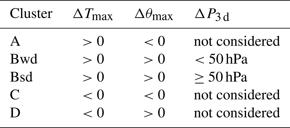
Hence, potential temperature changes along the trajectory path can only be caused by diabatic processes such as radiative heating or cooling or latent heat release during phase changes of water. Temperature changes along the trajectories can additionally occur due to adiabatic compression or expansion (right-hand side of Eq. 2) caused by vertical descent or ascent, respectively. The classification of the trajectories considers these aspects through the following definition of clusters (see Table 2 for an overview): cluster A has a positive temperature difference, i.e., an increase in temperature along the trajectory, but a negative potential temperature difference, which could be caused, e.g., by radiative cooling. Cluster B has positive temperature and potential temperature (diabatic heating) differences. This cluster B is split further in two subclusters that are distinguished by the maximum descent (or ascent) ΔP3 d in the 3 d prior to the heatwave day. If this value exceeds or equals 50 hPa, then the trajectory is in the Bsd cluster, where “sd” stands for strong descent. Otherwise, the trajectory is classified as Bwd, with “wd” indicating weak descent or even ascent if ΔP3 d<0. In cluster C both temperature and potential temperature changes along the trajectory are negative. Cluster D is composed of trajectories with a negative temperature difference and a positive potential temperature difference (diabatic heating) along the trajectory. Note that the vast majority of heatwave trajectories are associated with clusters A, Bwd and Bsd, and the remaining clusters C and D are thus not considered in detail in the remainder of this study.
Table 2Criteria for trajectory clusters following Zschenderlein et al. (2019) but with a different pressure criterion.
Finally, it should be noted that, although adiabatic and diabatic processes determine changes in temperature and potential temperature along a trajectory, for the local temperature change at the ground advection plays an important role, too (see again Eq. 2). This means that air parcels for which the temperature does not change substantially during transport can still lead to high temperatures at the target location if they originate in a warmer region.
We first provide a general overview of the temperature increase in Europe expected under RCP8.5 conditions in Sect. 3.1. Afterwards we compare general heatwave properties in historic and future simulations. A first impression of changes in the associated dynamics is given by composite plots of the 500 hPa geopotential height level during heatwave onsets (Sect. 3.2). We then analyze the origins of the different air parcel clusters associated with historic and projected future heatwaves, also in comparison to the climatology (Sect. 3.3). Finally, we take a closer look at future changes of dynamic and thermodynamic properties of the Lagrangian backward trajectories (Sect. 3.4).
3.1 Future temperature increase in Europe in summer
The 90th percentile of daily maximum temperature for mid-August (Fig. 1a) reveals a latitudinal dependence with higher values towards the south and generally higher values over land. Towards the end of the 21st century (Fig. 1b), the largest increases in this percentile (>10 K) occur over the central parts of Europe, while the increase is smaller over southern and northern Europe (mainly <9 K) and the British Isles (about 6 K). The smallest warming is projected over the ocean (<6 K), with a slightly higher temperature increase over the Mediterranean Sea compared to the North Atlantic. The average increase in the mean summer (JJA) temperature over land in the Euro-Atlantic region is reported to be between about 3–6 K (Chan et al., 2020), indicating that increase in the 90th percentile is amplified compared to this mean increase over most regions.

Figure 3Properties of heatwaves in future (orange) and historic (blue) time slices in the six European regions: (a) number of heatwaves per year and region, (b) heatwave days per year, and (c) heatwave duration (in days) with a minimum heatwave lifetime of 3 d. The significance of the difference in means between historic and future heatwaves per region has been tested with a two-sided Welch's t test with a significance level of 0.05. Significantly different means are marked by a star on the top of the plots.
Mean temperatures are calculated in the respective regions on detected heatwave days and compared to the climatological mean JJA temperatures in Fig. 2. The mean JJA temperatures are projected to increase in the future from about 4 K in BI (Fig. 2d) to about 8 K in WR (Fig. 2c). In BI, GI and IP (Fig. 2d–f), i.e., the regions that also cover large areas over the ocean, the temperature anomalies on heatwave days with respect to the mean JJA temperature for the future and historic time slices are of a similar magnitude as the future increase in the mean JJA temperature. This also indicates that the projected warming during heatwaves is similar to the average JJA temperature increase. In contrast, in the regions that cover more grid points over land, i.e., Sc, CE and WR (Fig. 2a–c), the temperature anomalies during heatwaves are higher than the future increase in mean JJA temperatures, and the anomalies increase even further in the future by about 1 K on average in Sc (Fig. 2a) and by about 2 K on average in CE and WR (Fig. 2b and c).
In general, we observe no or only minor differences between general heatwave properties in historic and future simulations (compare orange and blue boxes in Fig. 3). Similar to Zschenderlein et al. (2019), we find typical occurrences of zero to two heatwaves per year in most regions (Fig. 3a). The typical duration is generally less than 10 d but can reach maxima of up to about 20 d in IP in the historic time slice and about 45 d in GI and Sc in the future (Fig. 3c). In most regions, except for WR, the maximum duration increases in the future. Compared to Zschenderlein et al. (2019), the interquartile range of heatwave days per year is smaller, especially in WR (ca. 12 vs. 20) and CE (ca. 8 vs. 14), where the first number refers to the data presented in Fig. 3c and the second number is the approximate value from Zschenderlein et al. (2019) (their Fig. 4).
Since the method of heatwave detection is percentile-based, the total number of heatwave days is – as to be expected – almost identical in both time slices. However, in the future period we observe an increase in the number of heatwave days towards the end of July up to mid-August (see orange excess in Fig. S1 in the Supplement). Moreover, the future frequency distribution narrows with fewer heatwave days before mid-July. A fit with skew normal distributions shows an increase in skewness and a decrease in scale in the future distribution, i.e., a higher deviation from a normal distribution. The differences in mean and standard deviation between the two periods are statistically significant (see Supplement: Table S1 and Fig. S2).
A comparison of historic and future distributions of daily temperature maxima on heatwave days reveals that the distributions are primarily shifted towards higher temperatures but nearly do not change in shape (Fig. S3). However, there is a broadening of the distribution towards higher temperatures in BI (Fig. S3a) and a narrowing of the distribution in WR with an increase in peak probabilities by about 5 percentage points (Fig. S3f). Similar results are obtained for the distributions of the HWMId (see Supplement Fig. S4).
3.2 Composites of 500 hPa geopotential height for the first day of heatwaves
A first impression of the dynamical conditions leading to heatwaves and their projected future changes is provided through composites of the geopotential height fields at the 500 hPa level (Figs. 4 and 5). The composites based on the CESM-LE simulations for the historic time slice (left columns of Figs. 4 and 5) are similar to the results of Zschenderlein et al. (2019), who studied heatwaves in the ERA-Interim reanalysis data set in the period 1979 to 2016, both with regard to the mean and standard deviation patterns. In both data sets, the composites are characterized by ridges (positive anomalies) near the region affected by a heatwave with a relatively low standard deviation compared to the regions upstream and downstream of the ridges. However in the CESM-LE data, the ridge axis is located towards the east of the study areas for some regions (CE, BI and IP), whereas the axis appears to be more centered in the results of Zschenderlein et al. (2019). In our analysis as well as theirs, the most pronounced anomaly pattern resembles an Omega block over Scandinavia (Fig. 4a). Except for WR and GI, all regions are located west of the ridge and thus characterized by southwesterly flow in the CESM-LE data. Heatwaves in WR are also associated with an Omega-like pattern whose center is within the WR region (Fig. 5g). In IP and GI, the heatwaves are associated with extended subtropical ridges (Fig. 5i and k).
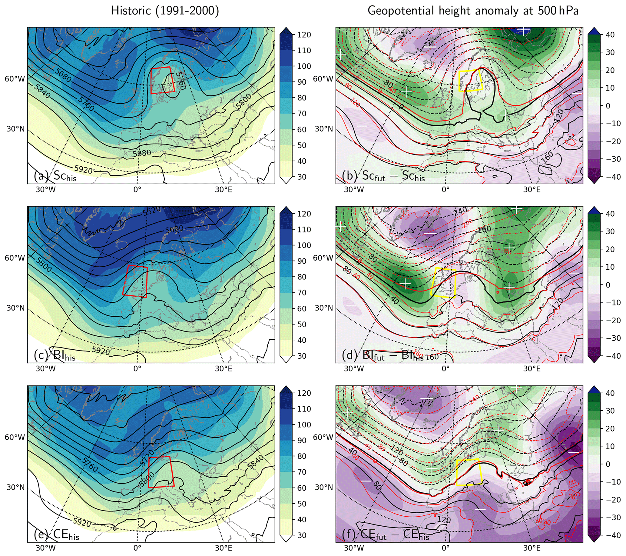
Figure 4Composites of the geopotential height fields at 500 hPa for the first day of heatwaves in different European regions: (a, b) Scandinavia (Sc), (c, d) British Isles (BI) and (e, f) Central Europe (CE). Panels (a), (c) and (e) refer to the historic time slice (1991–2000) with mean geopotential height (black contours, in geopotential meters, or gpm) and standard deviation (shaded, in gpm). Panels (b), (d) and (f) show the difference between the historic and future (2091–2100) mean geopotential anomaly fields at 500 hPa. For the calculation of these anomalies, the mean geopotential height for the first day of all heatwaves inside the respective area is first subtracted from the geopotential height composites. The resulting fields are shown by black (historic) and red (future) contours in the right column. The color shading then shows the difference between the two fields (future minus historic); violet (green) shading indicates areas of lower (higher) geopotential height in the future. Relative minima (maxima) of the difference fields (rough estimates) on the right column are labeled by minus (plus) signs.
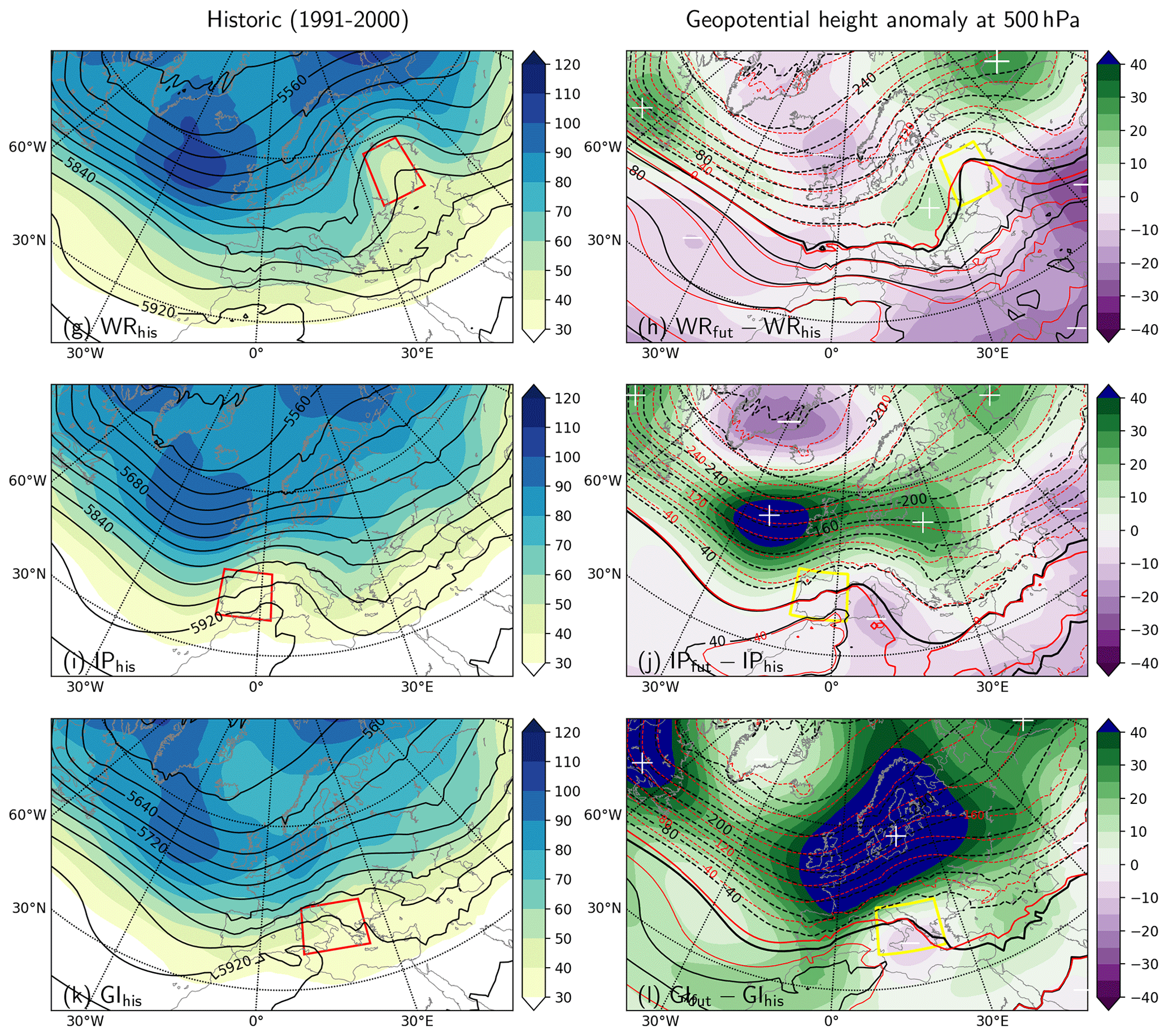
Figure 5As in Fig. 4 but for (g, h) Western Russia (WR), (i, j) the Iberian Peninsula (IB) and (k, l) Greece and Italy (GI).
Due to the temperature increase towards the end of the 21st century, the geopotential height of the 500 hPa level is expected to rise, too1. In order to facilitate the comparison between historic and future composites and to identify possible changes in the dynamic conditions, the mean geopotential height fields are plotted as anomalies on the right columns of Figs. 4 and 5. In general, the composite patterns remain remarkably similar between future and historic time slices (see also black and red contours on the right columns of Figs. 4 and 5). The anomaly patterns of all regions point towards a northward shift of the Atlantic westerly jet stream during future heatwaves (see Figs. 4 and 5). Furthermore, in all regions, the Icelandic low deepens in the future during heatwave onsets while the Azores high remains more or less unchanged, except for GI (see Fig. 5f showing a more pronounced Azores high and approximately unchanged conditions for the Icelandic low). However, the overall changes in the geopotential height anomalies of the 500 hPa level are relatively small, in the range of about ±40 gpm. This is about ±0.7 % of the typical height of the 500 hPa level2. On the other hand, composites of so many cases tend to smooth differences. In order to obtain more detailed insights into the relative roles of dynamical and thermodynamic changes for future heatwaves, we thus investigate these processes using a Lagrangian perspective based on backward trajectories.
3.3 Origins of air parcel trajectories associated with heatwaves
In order to identify the origins of the low-level air that is associated with heatwaves, we analyze the spatial distribution of backward trajectories initialized at heatwave locations 3 d prior to the heat event. These distributions are compared with typical origins of low-level air masses in summer (JJA). Furthermore, we investigate projected changes of the parcel origins in the future.
Figure 6 shows the origins of backward trajectories initialized in BI as well as their differences to the projected future changes. The trajectory densities for the climatology and future time slices are shown in Fig. S5. The majority of the parcel origins 3 d prior to the heatwaves are located east of the study region, mainly over the North Sea and Central Europe (Fig. 6a). This is in accordance with the ridge observed in the composite plot (Fig. 4c) that suggests reduced westerly and/or occasionally easterly winds towards the BI. A similar result was obtained by Zschenderlein et al. (2019) based on reanalysis data (their Fig. 7); however, in their case, the trajectory density is also higher directly in the BI region. The mainly easterly parcel origin is in sharp contrast to the JJA climatological origins of backward trajectories initialized over BI, most of which are located west of the BI and farther away over the North Atlantic (Figs. S5 and S6a). In the future, a shift of the parcel density peak towards the north of the BI and the surrounding ocean is projected, and fewer parcels are located southwest and southeast of the BI region (Fig. 6b). This shift – but much less pronounced – can also be found in the general JJA climatology (Fig. S6c). Together, these changes are associated with an even more pronounced difference between the origins of heatwave and climatological JJA trajectories in the future compared to the historic time slice (Fig. S6a and b).
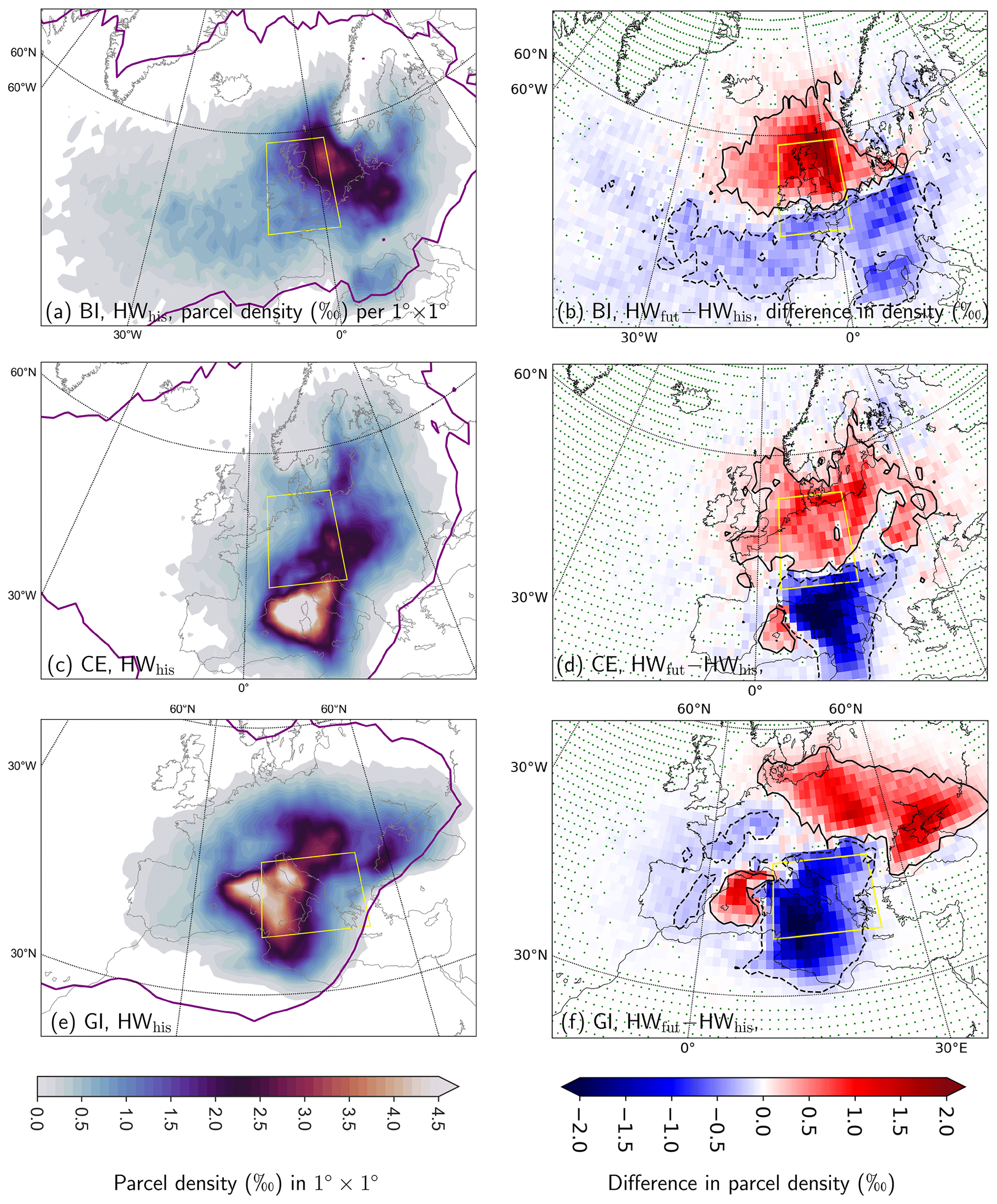
Figure 6Spatial distribution of the trajectories initialized during heatwaves in (a, b) BI, (c, d) CE and (e, f) GI. The left column shows the densities of the parcel trajectories (color shading) 3 d prior to the heatwaves. The purple contour indicates a parcel density (all trajectories) of 0.1 ‰ per 7 d prior to the heatwave; the right column shows the difference between future trajectory densities 3 d prior to the heatwaves HWfut minus the historic ones HWhis. Densities (in ‰) are shown by red–blue color shading. The solid (dashed) black contour in panels (b)–(e) marks the +0.2 ‰ (−0.2 ‰) difference in parcel density. The significance of differences in parcel densities was determined with a bootstrap method, obtaining 99 % confidence intervals at each grid point and for each period by resampling the original heatwave data 100 times with replacement. Grid points marked by a green dot show no significant difference in parcel densities between the two respective distributions.
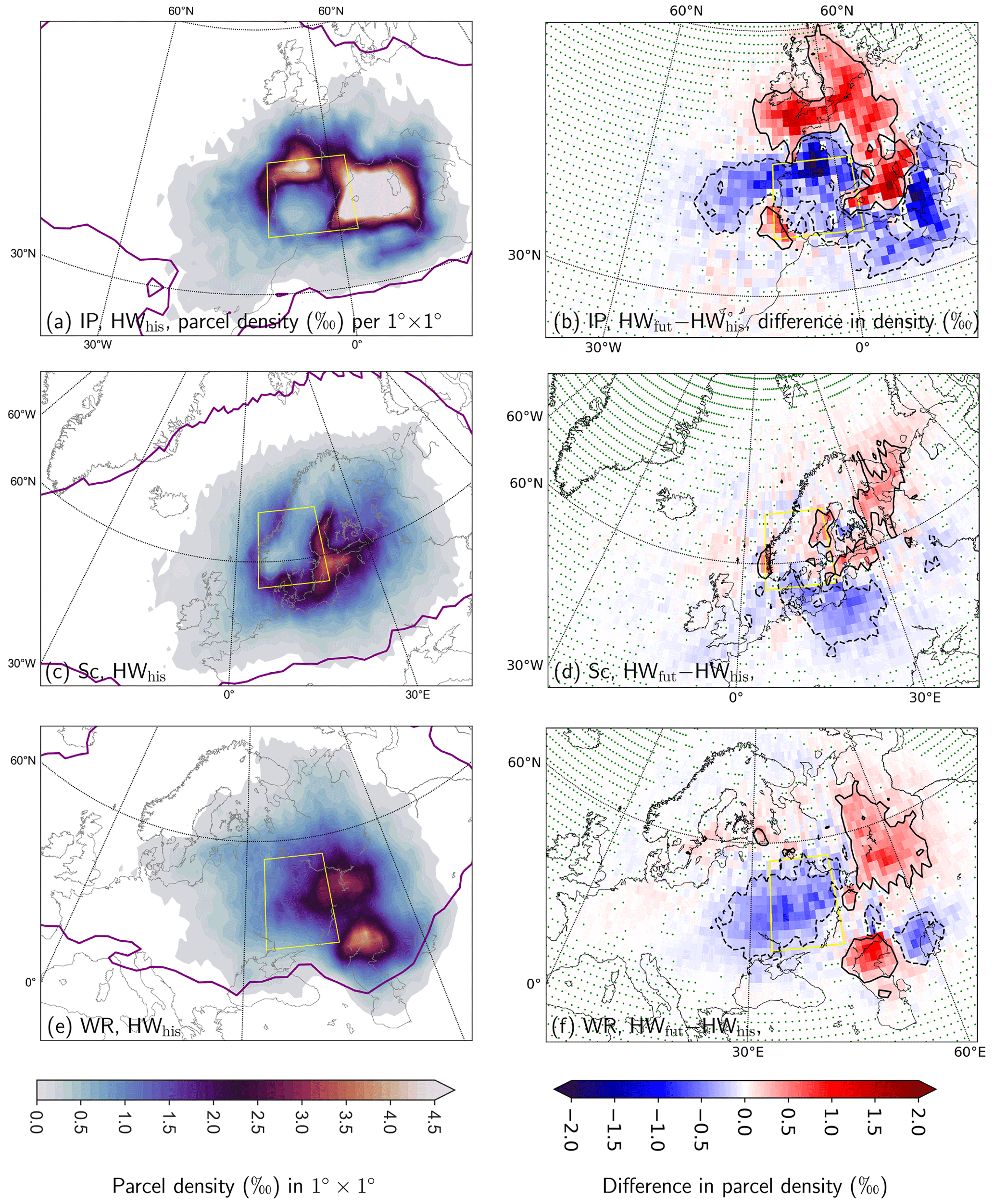
Figure 7As in Fig. 6 but for IP, Sc and WR.
In CE, most of the heatwave-related air parcels originate from the Mediterranean Sea south of the CE region 3 d prior to the heat event (Fig. 6c). High parcel densities are also found southeast of the CE region as well as generally east of CE. Compared to the results published in Zschenderlein et al. (2019) (their Fig. 7), the peak of the parcel density is shifted more southward in the CESM-LE data. Again, the mainly southerly and easterly parcel origins are in contrast to the general JJA climatology (Fig. S6d), which is associated with typical origins northwest of and partially in the northwestern part of the CE region. For the future, a northward shift of the parcel densities is projected, with a higher density inside the CE region, while the parcel density south of CE becomes smaller (Fig. 6d). Projected changes in the JJA climatological parcel origins are generally small, with only a slight increase in parcel densities northwest of the CE region (Fig. S6f), suggesting only minor future changes in the general summer circulation over CE.
GI is the only region where the air parcels associated with heatwaves originate mainly from the western part of the region, with the maximum parcel density over the Mediterranean Sea (Fig. 6e). However, there is another less pronounced peak in parcel densities north and northeast of the GI region. Overall, these results are similar to those published in Zschenderlein et al. (2019) for the GI region. In the JJA climatology, the peak in parcel origins in the western part of GI is less pronounced, and instead more air parcels have traveled over a longer distance from northern and western Europe towards GI (Fig. S6g). For future heatwaves, the peak in the western part of GI is projected to reduce, and more parcels originate from further north and northeast and from the western Mediterranean Sea east of the Spanish coast (Fig. 6f). Again, the difference between historic and future climatologies is only minor and implies a slight northward shift (Fig. S6)).
In the IP region, the air parcels associated with heatwave days originate mainly directly from the east of the region in the western part of the Mediterranean Sea but also from the northern parts of IP, with a density peak over the North Atlantic north of the Spanish coast 3 d prior to the heat event (Fig. 7a). This is also in accordance with Santos et al. (2015), who identify easterly/northeasterly flow with hotspots of parcel densities east and northeast of the Iberian Peninsula shortly before summer warm events in IP. Moreover, they found anticyclonic flow and high residence times over or near the IP (see Santos et al., 2015, their Fig. 5). Similar results are shown in Zschenderlein et al. (2019); however, their highest parcel densities were rather concentrated inside the IP region and extended only slightly to the north and east. Comparing the heatwave parcel densities with the JJA climatology, the parcel densities peak farther to the northwest of the region, and considerable lower densities are found east of the IP region in the climatology (Fig. S7a). In the future simulations, we observe a shift in parcel densities to the north (towards the channel) and east of the region and an increase in parcel density over the Mediterranean Sea (Fig. 7b). In the future summer climatology, the overall pattern follows that of the heatwaves but with less distinct changes (Fig. S7c).
Air parcel origins of Scandinavian heatwaves are mainly located east and south of the Sc region over the Baltic Sea (Fig. 7c). The locations of largest parcel density are comparable to Zschenderlein et al. (2019), but they found higher densities also inside the Sc region. The general JJA climatology indicates a typical westerly flow in summer in the Sc region, with fewer air parcels originating from the south and east compared to heatwave periods (Fig. S7d). For future heatwaves, the air parcel origins are projected to stay relatively unchanged, with only a slight shift towards the north (Fig. 7d). Also the summer climatology in the projected future is almost identical to the present-day distribution (Fig. S7f), leading to very similar differences between heatwave and climatological parcel origins in present-day and future climate (Figs. S7d and e).
In WR, the air parcels associated with heatwaves also originate from the east and southeast of the WR region (Fig. 7e). Zschenderlein et al. (2019) found similar results, although their southeasterly peak is even further shifted to the east. Note, however, that their results for WR were dominated by the exceptionally long-lasting heatwave in 2010. Again, the air parcel origin during heatwaves is in strong contrast to the JJA climatology, for which the typical flow comes from the northwest and west (Fig. S7g). For future heatwaves, a slight shift of parcel origins to the east is projected and an increase in the parcel density over the northern part of the Caspian Sea, but overall the changes are relatively small (<1 ‰) (Fig. 7f). Also, the changes during of the climatological air parcel origins are very small, with a slight tendency towards a northward shift (Fig. S7i).
3.3.1 Summary: parcel origins
The analysis of air parcel origins in this section has shown that most of the (boundary-layer) parcels associated with heatwaves stem from inside and/or close to the respective regions 3 d prior to the heat event. This is in accordance with the existing literature (e.g., Zschenderlein et al., 2019). Compared to the JJA climatology, air parcels associated with heatwaves move from the east into the respective regions, while the typical summer airstreams come from the west. An exception is GI, where the air associated with heatwaves also comes from the west of the region (western Mediterranean Sea). Furthermore, for the CE region, a considerable amount of air parcels originate south of CE, with a maximum over the western Mediterranean Sea. In accordance with the anticyclonic circulation anomalies (see again Sect. 3.2), median parcel trajectories typically follow an anticyclonic curvature in the last 3–5 d prior to the heat event in the vicinity of the respective regions (not shown). In future heatwaves, parcel origins generally tend to shift northward in BI, CE, GI and IP. For Sc and WR, projected future changes are small, with a minor tendency towards an eastward shift. Interestingly, air parcel origins for the entire summer climatology are not projected to change much, which implies only minor changes in the typical summer circulation.
3.4 Physical characteristics of heatwave trajectories
To study the physical characteristics of airstreams associated with European heatwaves, the trajectories are categorized into different clusters as described in Sect. 2.4 (see also Table 2). The majority of all trajectories – independent of the region, time slice and heatwave classification – fall into the cluster categories A or B (Bwd, Bsd), which means that along almost all (>90 %) trajectories the temperature increases (Fig. 8). However, the exact partitioning between clusters A, Bwd and Bsd differs between the European regions. Regions close to the ocean (BI, GI, IP) have a higher percentage of trajectories in cluster A (see red lines in Fig. 8), which is characterized by diabatic cooling. While cluster A is least important in WR with only about 10 %, the Bwd and Bsd clusters have a larger share in this region. The B clusters are characterized by diabatic heating along the trajectory. Furthermore, air parcels in cluster Bsd strongly descend by more than 50 hPa in the 3 d prior to the starting date of the backward trajectory. The largest fraction of parcels in the Bsd cluster compared to all other regions is found in WR. Compared to the JJA climatology, heatwaves are characterized by a higher percentage of air parcels in the cluster A and a much lower fraction in cluster Bwd in BI, GI and IP, the regions that are affected by the North Atlantic or Mediterranean Sea. In the other regions (CE, Sc and WR) a much higher percentage of parcels fall into the Bsd category during heatwaves compared to the JJA climatology. Comparing historic and future heatwaves, we observe a decrease in cluster A trajectories in CE, WR and GI, while the fraction of cluster Bsd trajectories increases in the same regions and additionally in Sc (yellow lines in Fig. 8). Furthermore, the fraction of air parcels in cluster Bwd increases by about 10 (≈5) percentage points in CE (GI) (blue lines in Fig. 8).
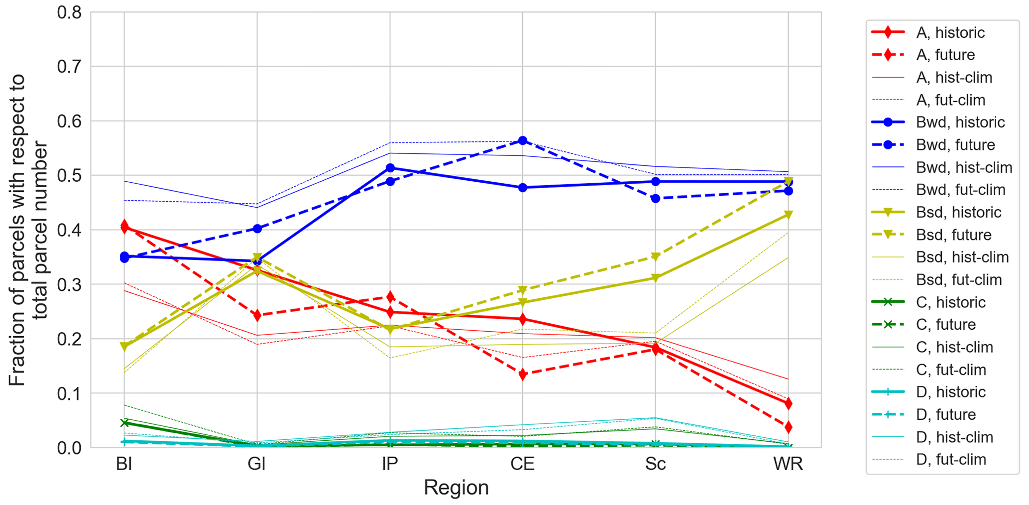
Figure 8Fraction of trajectories that belong to the different clusters A, Bwd, Bsd, C and D introduced in Sect. 2.4 per region and time slice (solid lines belong to historic data and dashed lines to future data). Displayed are the fractions for heatwave trajectories (bold lines) as well as for the general summer (JJA) trajectories (thin lines). The regions are ordered according to the fraction in cluster A. Note that the lines connecting the different regions are only plotted to simplify the identification of the clusters and possess no physical meaning.
Figure 9 shows the median pressure along air parcel trajectories that fall in clusters A, Bsd and Bwd. Cluster A, which is characterized by diabatic cooling, shows the strongest descent over the 10 d period in all regions, although the pressure at h differs between about 700 hPa in BI (Fig. 9a, yellow lines) and about 500 hPa in WR (Fig. 9d, yellow lines). The lowest altitude (highest pressure) 10 d prior to the heatwave is found for the median of cluster Bwd, where the parcels first slightly descend for about 7 d until they are close to the surface and then either ascend (in Sc, CE and IP) or remain almost at the same pressure level (in BI, WR and GI; see Fig. 9, blue lines). The median pressure evolution of the Bsd cluster (Fig. 9, red lines) is characterized by an almost constant vertical level for about 6 to 7 d prior to the heatwave at an intermediate pressure of about 750 hPa in most regions. Exceptions are BI with ≈820 hPa (Fig. 9a) and WR with about 700 hPa (Fig. 9d). The last 3 to 4 d prior to the heatwave event are then characterized by a strong descent in the Bsd cluster with a median change in pressure larger than 100 hPa in all regions. Compared to the typical JJA climatology 10 d before parcels reach the regions, the largest differences in the median pressure are found in regions Sc, CE, WR and IP. In all regions and clusters, except of cluster A in BI and GI, the JJA parcels start from a lower height, and their descent is not as strong as in the heatwave cases. Differences in the median pressure evolution between future and historic heatwaves in the six European regions are mostly small (bold dashed and solid lines in Fig. 9). The largest changes are projected in WR (cluster A) and IP (all clusters). In WR, we observe a stronger descent in cluster A shortly before the heatwave event and a higher starting point 10 d prior to the heatwave. However, the fraction of parcels in cluster A in region WR is very low (<0.05; see Fig. 8) in the future. In IP (Fig. 9e) the median pressure of air parcels in all three clusters is lower for future heatwaves 10 d prior to the event. Moreover, the historic and future JJA pressure medians are almost identical.
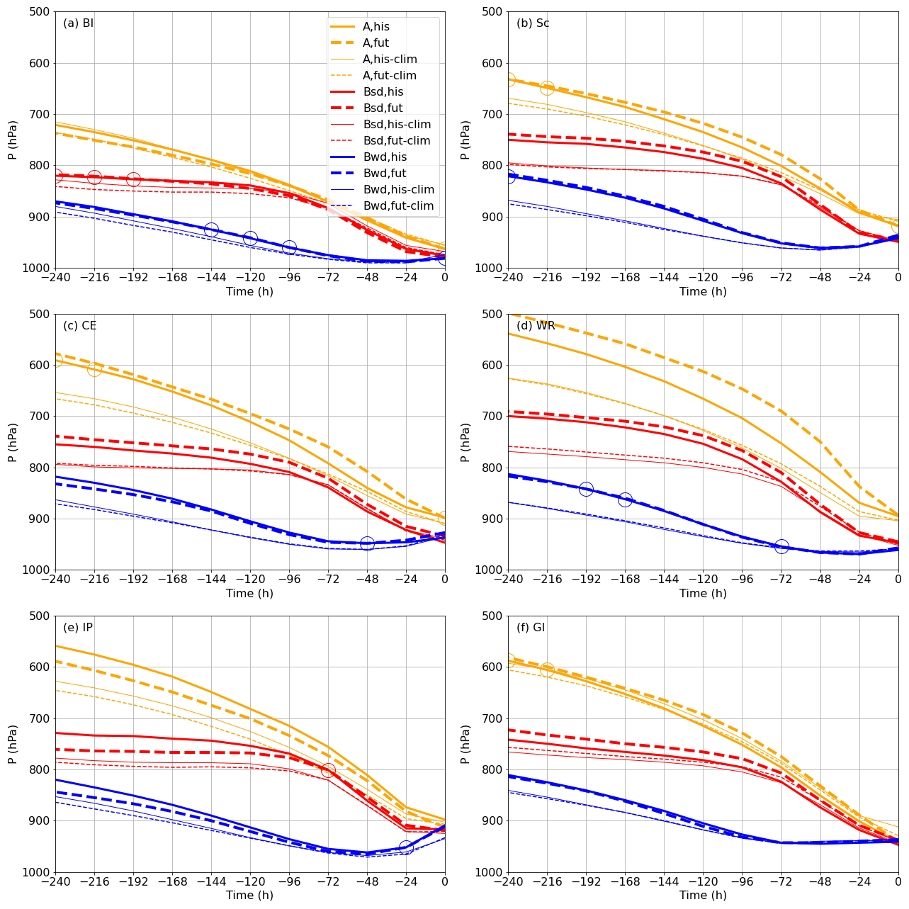
Figure 9Median evolution of pressure (hPa) along the air parcel trajectories in clusters A, Bsd and Bwd in the six European regions. Bold solid (bold dashed) lines represent the air parcels associated with a heatwave event in the historic (future) time slice; accordingly the thin lines show the climatological JJA values. A significance test (Welch's t test) was performed with a significance level (p value) of 0.05. Large, open circles in the plots indicate insignificant (p values > 0.05) differences between the medians of future and historic heatwaves.
The median development of temperature and potential temperature along the trajectories is displayed in Fig. 10 for heatwave days as well as for the JJA climatology. Jointly analyzing these two variables allows us to distinguish between future changes in adiabatic and diabatic warming processes (see again Sect. 2.4). Overall, for the JJA climatology (thin solid and dashed blue lines in Fig. 10), the median temperature and potential temperature evolution stays similar between the historic and future time slices for clusters A and Bsd, while a stronger diabatic heating (of less than 5 K) is projected for cluster Bwd in most regions. On the other hand, the evolution differs strongly between heatwave and JJA trajectories, with larger temperature changes (difference ≈ 10 K) for the heatwave trajectories. In the following, the median distributions associated with heatwave days in the three clusters as well as their future changes are discussed in detail. In general, cluster A (yellow lines in Fig. 10) shows the largest temperature increase in the 10 d period prior to the heatwave event (except for the BI). The magnitude of this increase depends strongly on the region and is largest in WR with about 35 K (historic) to 40 K (future) (vs. 25 K increase in the JJA climatology) and smallest in BI with about 15 K. Moreover, the potential temperature evolution of cluster A shows that the air parcels undergo diabatic cooling of about 7 K (up to 10 K in WR) and in some regions diabatic heating right before the heatwave event (last 24 h before the event in WR, CE and Sc, Fig. 10b–d). Cluster Bsd (red lines in Fig. 10) is characterized by approximately adiabatic () warming between day 10 and about day 2 prior to the heatwave in most regions. In the two clusters, Bsd and A, of heatwave-associated air parcels there are only minor differences between future and historic time slices in BI, Sc and IP but stronger temperature increases in WR, CE and GI. This temperature increase is larger (between about 2–5 K in most regions) than the one – if any – observed in the summer climatology. Air parcels in cluster Bwd (blue lines in Fig. 10) are generally heated (increase in both temperature and potential temperature) over the whole 10 d period, with stronger diabatic heating directly before the heatwave event. These Bwd parcels are characterized by weak descent, and, hence, they are affected by boundary-layer processes such as surface–atmosphere interactions over a long period of time. Diabatic heating happens preferentially through surface fluxes; this is why the air parcels with the weakest descent (that are closer to the surface for a longer period) experience the strongest diabatic heating. An exception is BI, where the Bwd parcels are first cooled for a few days and then heated in the last days prior the heatwave (Fig. 10). The diabatic heating of the Bwd parcels over the 10 d is between about 7 K in BI up to about 10 K in WR, CE, IP and GI for historic heatwaves and becomes even larger in these regions in the future (about 15 K). This increase in diabatic heating for the heatwave trajectories is similar to the increase projected for the JJA climatology. Altogether, more pronounced future changes in adiabatic and diabatic heating (the latter primarily in cluster Bwd) are projected in the regions with continental climate, in particular CE and WR, compared to those closer to the ocean.
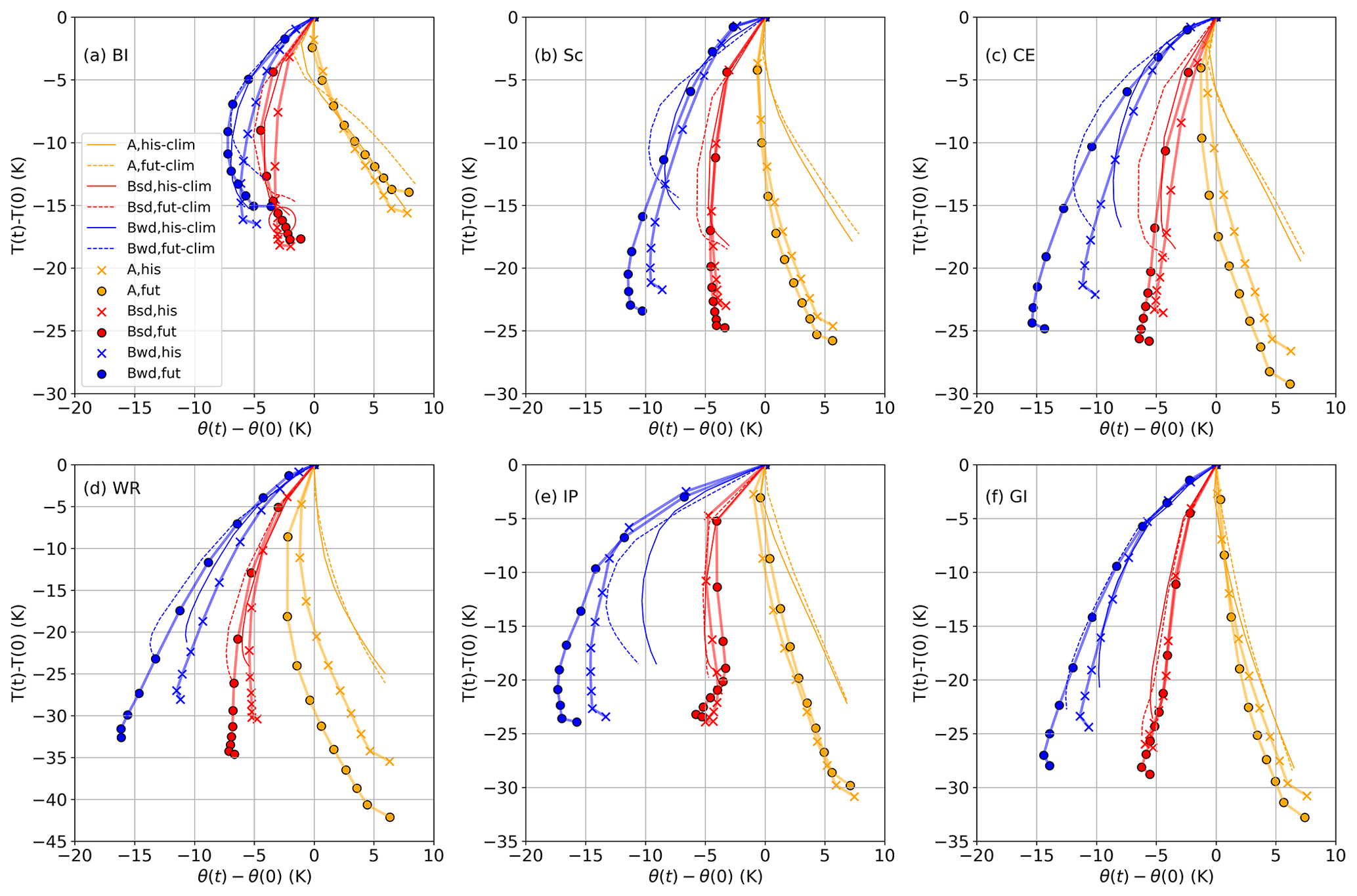
Figure 10Median temperature and potential temperature evolution along the air parcel trajectories for each cluster (A: yellow; Bsd: red; and Bwd: blue) relative to the values on the heatwave day in the six European regions, i.e., the point with coordinates (0, 0). Dots and crosses indicate the values in intervals of 24 h, always at 12:00 UTC. Note the different ranges of the temperature axis (y axis) for the different regions. Thin lines correspond to historic (solid) and future (dashed) climatological medians. A significance test (Welch's t test) was performed with a significance level (p value) of 0.05. Large, open circles in the plots indicate insignificant (p values > 0.05) differences between the medians of future and historic heatwaves.
In Fig. 11, an example of the entire distribution of the trajectory properties ΔTmax and Δθmax is plotted for the CE region. The scatterplot (Fig. 11a) shows that the majority of the strongly descending air parcels (blue colors) falls in cluster A. Strongly descending parcels can also be found for large temperature increases and weak diabatic heating in cluster B. Strongly ascending parcels ( hPa) are connected with strong diabatic heating and weak temperature changes in either cluster B or C. The majority of all parcels associated with heatwave days in CE are in cluster B with temperature increases ΔTmax between approximately 20 and 40 K and diabatic heating Δθmax up to about 20 K in the historic time slice (Fig. 11b) and up to about 30 K in the future time slice (Fig. 11c). With respect to the thermodynamic properties of the parcels, we thus observe a future shift towards increased diabatic heating along the parcel trajectory in CE (cluster B, Fig. 11d). Additionally, we find an increase in the number of parcels with a larger temperature increase in the future (also cluster B) and an overall smaller probability for parcels in cluster A. The distributions of the other European regions, except of BI, are similar to the CE plots; however, the details differ from region to region (see Figs. S8 and S9 for similar plots for the other regions and first column in Figs. 12 and S10). For example, we observe a higher number of strongly descending parcels in GI in cluster A and an increasing probability of cluster A in IP and BI in the future that is not observed in the other regions. This increase in cluster A is also in accordance with Fig. 8, which showed a higher fraction of that cluster in the future in these two regions.
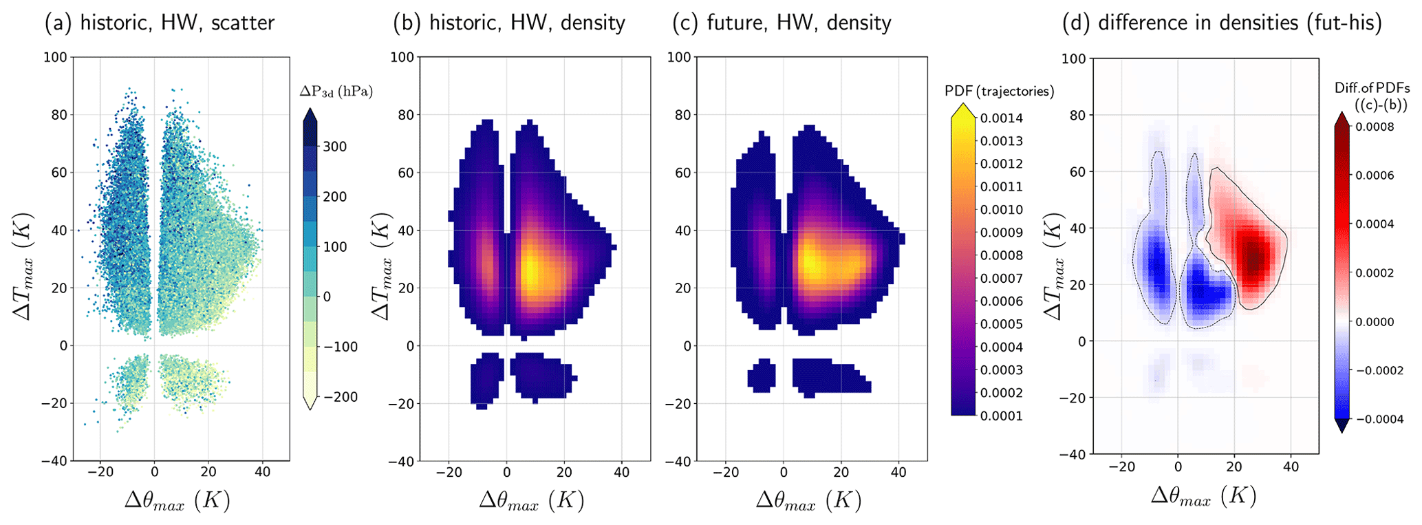
Figure 11Maximum temperature difference ΔTmax along trajectories associated with heatwaves plotted against their maximum potential temperature difference Δθmax for the CE region. (a) Scatterplot with each dot representing the properties of one trajectory; descent/ascent in the 3 d prior to the heatwave ΔP3 d is indicated by colors; (b, c) probability density function (PDF; Gaussian kernel-density estimate) of trajectory counts (b) in the historic time slice and (c) in the future time slice. Violet to yellow colors show the probability in grid boxes of 2 K × 2 K. Probabilities < 0.00001 are omitted. (d) Difference between PDFs shown in panel (b) minus panel (c); absolute values of probability differences smaller than <0.000001 are omitted. Solid (dashed) black contour marks a value of +0.00005 (−0.00005) of the difference in PDFs.
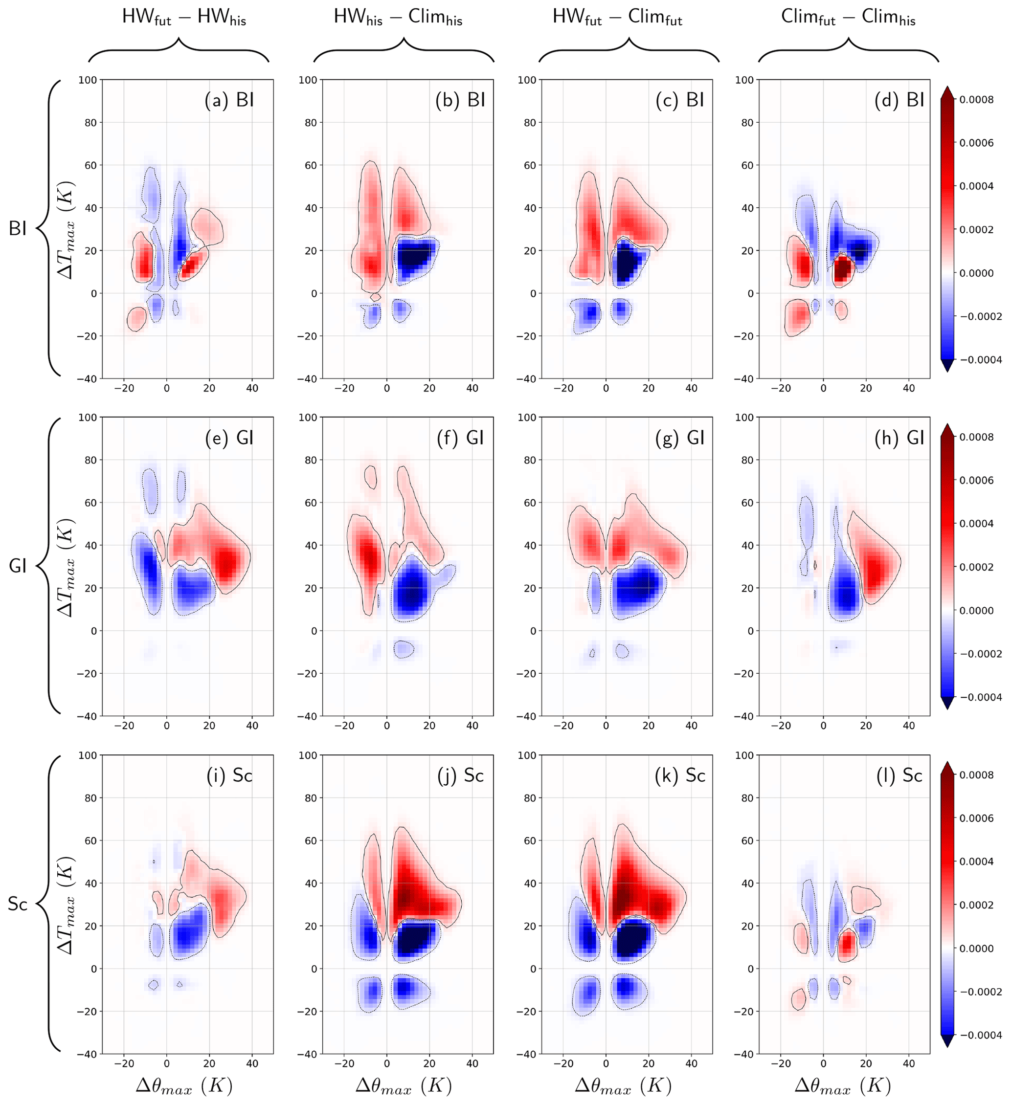
Figure 12Maximum temperature difference ΔTmax along trajectories plotted against the maximum potential temperature difference Δθmax for (a–d) BI, (e–h) GI and (i–l) Sc. Displayed is the difference between PDFs (as in Fig. 11d). Different regions are shown in rows (four figures per region), and several different plots are shown in columns: (a, e, i) difference between future and historic heatwave distributions; (b, f, j) historic heatwave PDF minus historic climatological JJA PDF; (c, g, k) future heatwave PDF minus future, climatological JJA PDF; and (d, h, l) difference between future and historic climatological JJA PDFs. The probability has been calculated in grid boxes of 2 K × 2 K, and absolute values of probability differences smaller than <0.000001 are omitted. Solid (dashed) black contour in panel (d) marks a value of +0.00005 (−0.00005) of the difference in PDFs.
The general pattern of increasing diabatic heating for medium-range temperature increases (up to about 40 K) also occurs in the general JJA climatology (fourth column in Figs. 12 and S10, especially in GI, CE, IP and WR). However, compared to the general JJA climatology, the heatwave trajectories are shifted towards larger temperature increases (max(T)>20 K) (all regions in clusters A and B; see second and third columns in Figs. 12 and S10). Moreover, the parcel distributions of future and historic heatwaves are additionally shifted towards larger diabatic heating (max(Θ)>20 K) (all regions except for BI) compared to their respective climatologies.

Figure 13Trajectory properties of clusters (defined in Sect. 2.4) calculated on heatwave days in comparison to climatological (JJA) values in different European regions: (a–d) BI, (e–h) Sc and (i–l) WR. The top row shows the difference in pressure ΔP3 d 3 d prior to the heat event/prior to arrival in the target region, the second row from top shows the maximum change in potential temperature Δθmax along the trajectory, the third row from top is the maximum change in temperature ΔTmax along the trajectory and the bottom row is the potential temperature 7 d prior to the arrival in the respective region. Historic (light purple, third boxes) and future (red, fourth boxes) refer to air parcels started on heatwave days; historic_clim (green, first boxes) and future_clim (yellow, second boxes) show the JJA climatology. Black stars above the boxes indicate that the difference between the means of either future and historic heatwaves or climatologies is insignificant (p value of 0.05 based on a t test). All other means are significantly different.
Trajectory properties are displayed as boxplots for the respective clusters in Figs. 13 and S11 in order to further summarize and compare future and historic heatwaves as well as climatological JJA conditions. BI is the only region where we see no difference in the thermodynamic properties such as maximum increase in temperature (Fig. 13c), maximum increase in potential temperature (Fig. 13b) and maximum descent in the 3 d prior to the initiation of the trajectory (Fig. 13a) between the heatwaves and climatologies. However, we observe large differences in the potential temperature distribution 7 d (−168 h) prior to the initiation of the backward trajectory (Fig. 13d). There is nearly no overlap of the interquartile ranges between the heatwaves and the respective climatologies as well as between historic and future heatwave air parcels. This implies that the air originates from higher altitudes with larger potential temperature values and/or from a region with higher-than-usual temperatures. For BI, in particular the latter is important (enhanced transport form continental regions in the east, which are particularly warm in summer; see again Fig. 6), as the pressure level at −168 h does not differ strongly between heatwaves and climatology (see again Fig. 9). Similar results with respect to the potential temperature 7 d prior to initialization are found in all other European regions (Figs. 13 and S11d, h, l). Nevertheless, for the other regions also variations in the pressure at −168 play a more important role (Fig. 9). Moreover, in the other European regions, heatwave trajectories differ from their climatological counterparts also with respect to the other thermodynamic properties shown in Fig. 13. For example, air parcels in cluster A (e.g., in Sc and WR; see Fig. 13e and i) experience stronger subsidence than the climatology. This difference in subsidence in cluster A even increases in the future heatwaves (red boxes), in particular for WR (Fig. 13i). This larger subsidence coincides with a larger increase in temperature along the trajectories (e.g., Fig. 13g and k), and hence this increase can be attributed to the adiabatic compression of the parcels that overcompensates for the diabatic cooling.
3.4.1 Summary: characteristics of air parcels
In summary, future heatwaves are projected to intensify due to (i) increased diabatic heating (all regions, except for BI), (ii) increased descent and adiabatic warming (mainly regions WR, CE and Sc) and (iii) warmer air parcels already prior to transport to the heatwave region (all regions). Point (iii) corresponds to the overall increase in summer temperature, and a similar warming can thus also be observed for other trajectories not necessarily related to heatwaves (JJA climatology). In contrast, points (i) and (ii) can be specific or amplified for heatwaves, such as the enhanced diabatic heating in WR, CE, GI, and SC in cluster Bwd and the enhanced descent and adiabatic warming in cluster A. These processes can thus lead to an intensification of heatwaves beyond the average summer warming.
In this work, we have analyzed dynamical and thermodynamical mechanisms associated with European heatwaves and their projected future changes based on Lagrangian air parcel trajectories. In order to properly cover the influence of natural variability, heatwaves are identified in a large single-model ensemble of climate simulations (CESM-LE data with 35 members, Kay et al., 2015) for two time slices, 1991-2000 (historic) and 2091–2100 (RCP8.5), based on the Heat Wave Magnitude Index daily (HWMId) – a percentile-based method introduced by Russo et al. (2015). This percentile-based index allows for a comparison of heatwaves in both time slices with each other since it relates the heat event to the underlying climatology and hence accounts for an expected anthropogenic temperature increase in the future. Moreover, the Lagrangian analysis permits the investigation of the origin of near-surface air masses associated with heatwaves and the study of the thermodynamic processes along their transport pathways. Our main goals have been to investigate the role of dynamic and thermodynamic aspects of heatwaves and how these might change in the future. In the following, we summarize and briefly discuss our main results, also in comparison to recent literature.
-
Minor changes in the general heatwave characteristics in most European regions. The percentile-based identification of heatwaves via the HWMId is – as expected – remarkably robust in both time slices with respect to the number of heatwave days and the heatwave duration in all regions, except for BI, where an increase in the number of consecutive heatwave days is projected. This is also in accordance with Vogel et al. (2020), who state that “for fully moving thresholds, no or only very few significant changes in heatwave characteristics with increasing warming levels are projected”. Additionally, we observe a significant, albeit small, shift of the heatwave peak towards the end of July and beginning of August in BI, CE, and IP and a significant, but small, narrowing of the heatwave season in CE, GI and WR.
-
Origins of heatwave near-surface air. In general, the core origin regions of the near-surface air masses that contribute to the heatwaves lie to the east of the respective region 3 d prior to the heatwave. More precisely, these core regions are located southeast of the northerly subregions and northeast of the southerly subregions (and in GI even partially to the west). This is in broad agreement with Zschenderlein et al. (2019), who, however, found higher trajectory densities within the region affected by the heatwave itself. Nonetheless, our results also indicate that the air is located close to the analyzed region where the heatwave occurs and is not advected from remote (warmer) regions. This is in line with Bieli et al. (2015), who also found short transport distances for heatwave-related trajectories. In comparison to the climatological transport pathways of near-surface air in summer, the heatwave air parcels origin closer to the regions of interest a few days prior to the heat event and travel slower. Furthermore, the model projections indicate a northward shift of heatwave-associated air parcel origins 3 d prior to the heatwave in the simulated future climate, with higher densities mainly north of and inside (BI, CE) the regions and reduced densities to the south of (and inside for IP, GI) the respective regions. This northward shift in the future can also be seen in the JJA climatology of most regions, however with smaller magnitude, such that the changes in the climatological parcel origins are mostly very small.
-
Projected changes in dynamic and thermodynamic air parcel properties relevant for future heatwaves. Our main findings show a diverse picture of changes in future heatwave characteristics across Europe. In some European regions such as Sc, CE and WR, we find a stronger temperature increase on heatwave days than would be expected because of the increase in mean summer temperature alone. This indicates that additional dynamic or thermodynamic processes amplify the intensification of heatwaves in some parts of Europe. Indeed, in these regions the subsidence during heatwaves is projected to increase in the future simulations, especially in the last 2–5 d prior to the arrival in the heatwave region, which is associated with amplified adiabatic warming. Moreover, in all regions except for BI the diabatic heating is projected to intensify. The latter affects air parcels located near the surface, and such boundary-layer diabatic temperature changes are likely driven by sensible heat fluxes that are enhanced when heatwaves co-occur with larger soil moisture deficits, especially in plain regions (Stéfanon et al., 2014; Schumacher et al., 2019). During heatwaves, the land surface can be expected to become drier in the future (Seneviratne et al., 2010); thus, the amplified diabatic heating may be due to an increase in the Bowen ratio, as also suggested by, e.g., Rasmijn et al. (2018) for WR. Additionally, the enhanced land–sea temperature contrast in a warming climate may play a role for this increased diabatic heating, as many air parcels move from the ocean towards the continent and thus directly experience this enhanced contrast. However, this change in land–sea temperature difference cannot fully explain the amplification of heatwaves beyond the seasonal mean warming projected in some regions, and it is also not totally independent of the surface drying mechanism mentioned before, as changes in continental temperature and humidity in a warming climate are coupled to each other (Byrne and O'Gorman, 2018).
A caveat of our analysis is that it is based on a single climate model only. However, we need high-resolution output on model levels for our trajectory calculations, and hence these analyses cannot easily be performed based on other model simulations, e.g., from the CMIP6 archive. Nevertheless, our comparison with the results of Zschenderlein et al. (2019), whose analysis is based on ERA-Interim reanalysis data, indicates that CESM1 captures the basic dynamics of European heatwaves reasonably well, which gives confidence in the corresponding future projections.
Finally, we want to add some final remarks with regard to the recent summer 2022 heat records. On 19 July 2022, Great Britain reported 40.2 ∘C at Heathrow Airport, London (Carrington, 19-). In the CESM-LE simulations presented here, the BI distribution shows maximum temperatures of up to 37 ∘C in the historic time slice (1991–2000) and up to about 48 ∘C in the future time slice (2091–2100). Assuming a linear increase, Heathrow's temperature record lies at the upper end of the expected range for the 2020s, which is also in accordance with the work of Christidis et al. (2020), who showed that events like the heatwave in July 2022 are possible but rare and will increase towards the end of this century. This shows that heatwaves are already changing in the direction as projected for the end of the century by CESM-LE and other global climate models. Our results provide guidance for upcoming changes in heatwave characteristic that could be used to improve adaptation measures for future heat events.
In summary, we have identified thermodynamic as well as dynamic contributions that are relevant for the future amplification of heatwaves in different European regions. In particular for Scandinavia, Central Europe and Western Russia, these processes lead to an increase in heatwave temperatures beyond the mean summer warming. Part of this amplification is due to increased diabatic heating in the boundary layer, which is likely linked to surface drying and enhanced sensible heat fluxes. Additionally, the excess heating is related to altered atmospheric dynamics, in particular enhanced descent of the air masses leading to stronger adiabatic warming in the simulated future climate, which is in some contrast to previous findings by Vogel et al. (2020), who suggested that changes in dynamics should be of minor importance.
The presented work provides a comprehensive overview of the range of future changes in heatwave characteristics in different European regions from a Lagrangian point of view and can serve as a starting point for further research. Nevertheless, the topic still needs further investigations, e.g., with respect to the robustness of the findings in other climate models.
The code of the CESM version 1 that was used for the Large Ensemble simulation is available from https://www.cesm.ucar.edu/models/cesm1.0/ (UCAR, 2020). The code of the trajectory model LAGRANTO is available from https://iacweb.ethz.ch/staff/sprenger/lagranto/download.html (Atmospheric Dynamics Group et al., 2020). Model output is available upon request from the authors.
The supplement related to this article is available online at: https://doi.org/10.5194/wcd-3-1439-2022-supplement.
LS and SP designed the study. LS produced the results and figures. LS and SP discussed the results and both contributed to the writing.
At least one of the (co-)authors is a member of the editorial board of Weather and Climate Dynamics. The peer-review process was guided by an independent editor, and the authors also have no other competing interests to declare.
Publisher's note: Copernicus Publications remains neutral with regard to jurisdictional claims in published maps and institutional affiliations.
This article is part of the special issue “Past and future European atmospheric extreme events under climate change”. It is not associated with a conference.
The authors would like to thank the HPC service of ZEDAT, Freie Universität Berlin (HPC system Curta; see Bennett et al., 2020, for details), for providing computational resources. Furthermore, we are grateful to Urs Beyerle (ETH Zurich) for performing the CESM-LE reruns and to Matthias Röthlisberger (ETH Zurich) for helpful discussions. We thank two anonymous reviewers and the editor for their helpful comments.
This research has been supported by the German Federal Ministry of Education and Research (Bundesministerium für Bildung und Forschung, BMBF) in its strategy Research for Sustainability (FONA) in the framework of subproject A5 of the ClimXtreme program (DynProHeat, grant no. 01LP1901C).
This paper was edited by Tim Woollings and reviewed by two anonymous referees.
Atmospheric Dynamics Group, Institute for Atmospheric, and Climate Science, ETH Zürich: LAGRANTO The Lagrangian Analysis Tool, https://iacweb.ethz.ch/staff/sprenger/lagranto/download.html (last access: 20 December 2022), 2020. a
Bennett, L., Melchers, B., and Proppe, B.: Curta: A General-purpose High-Performance Computer at ZEDAT, Freie Universität Berlin, https://doi.org/10.17169/refubium-26754, 2020. a
Bieli, M., Pfahl, S., and Wernli, H.: A Lagrangian investigation of hot and cold temperature extremes in Europe, Q. J. Roy. Meteorol. Soc., 141, 98–108, https://doi.org/10.1002/qj.2339, 2015. a, b, c, d, e
Breshears, D. D., Fontaine, J. B., Ruthrof, K. X., Field, J. P., Feng, X., Burger, J. R., Law, D. J., Kala, J., and Hardy, G. E. S. J.: Underappreciated plant vulnerabilities to heat waves, New Phytol., 231, 32–39, https://doi.org/10.1111/nph.17348, 2021. a
Brunner, L., Schaller, N., Anstey, J., Sillmann, J., and Steiner, A. K.: Dependence of Present and Future European Temperature Extremes on the Location of Atmospheric Blocking, Geophys. Res. Lett., 45, 6311–6320, https://doi.org/10.1029/2018GL077837, 2018. a
Byrne, M. P. and O'Gorman, P. A.: Trends in continental temperature and humidity directly linked to ocean warming, P. Natl. Acad. Sci. USA, 115, 4863–4868, 2018. a
Carrington, D.: Day of 40C shocks scientists as UK heat record “absolutely obliterated”, https://www.theguardian.com/environment/2022/jul/19/day-of-40c-shocks-scientists-as-uk-heat-record-absolutely, last access: 19 July 2022. a
Catalano, A., Loikith, P., and Neelin, J.: Diagnosing Non-Gaussian Temperature Distribution Tails Using Back-Trajectory Analysis, J. Geophys. Res.-Atmos., 126, e2020JD033726, https://doi.org/10.1029/2020JD033726, 2021. a
Chan, D., Cobb, A., Zeppetello, L. R. V., Battisti, D. S., and Huybers, P.: Summertime temperature variability increases with local warming in midlatitude regions, Geophys. Res. Lett., 47, e2020GL087624, https://doi.org/10.1029/2020GL087624, 2020. a
Christidis, N., McCarthy, M., and Stott, P.A.: The increasing likelihood of temperatures above 30 to 40 ∘C in the United Kingdom, Nature Commun., 11, 1–10, 2020. a
Fischer, E. M., Seneviratne, S. I., Vidale, P. L., Lüthi, D., and Schär, C.: Soil Moisture–Atmosphere Interactions during the 2003 European Summer Heat Wave, J. Climate, 20, 5081–5099, https://doi.org/10.1175/JCLI4288.1, 2007. a
Forzieri, G., Bianchi, A., e Silva, F. B., Herrera, M. A. M., Leblois, A., Lavalle, C., Aerts, J. C., and Feyen, L.: Escalating impacts of climate extremes on critical infrastructures in Europe, Global Environ. Change, 48, 97–107, https://doi.org/10.1016/j.gloenvcha.2017.11.007, 2018. a
Guo, Y., Gasparrini, A., Armstrong, B. G., Tawatsupa, B., Tobias, A., Lavigne, E., Coelho, Z. S., Pan, X., Kim, H., Hashizume, M., Honda, Y., Guo , Y.-L. L., Wu, C.-F., Zanobetti, A., Schwartz, J. D., Bell, M. L., Scortichini, M., Michelozzi, P., Punnasiri, K., Li, S., Tian, L., Osorio, S., Garcia, D., Seposo, X., Overcenco, A., Zeka, A., Goodman, P., Dang, T. N., Van Dung, D., Mayvaneh, F., Hilario, P., Saldiva, N., Williams, G., and Tong, S.: Heat wave and mortality: a multicountry, multicommunity study, Environ. Health Perspect., 125, 087006, https://doi.org/10.1289/EHP1026, 2017. a
IPCC: Summary for Policymakers, in: Climate Change 2021: The Physical Science Basis, Contribution of Working Group I to the Sixth Assessment Report of the Intergovernmental Panel on Climate Change, edited by: Masson-Delmotte, V., Zhai, P., Pirani, A., Connors, S., Péan, C., Berger, S., Caud, N., Chen, Y., Goldfarb, L., Gomis, M., Huang, M., Leitzell, K., Lonnoy, E., Matthews, J., Maycock, T., Waterfield, T., Yelekci, O., Yu, R., and Zhou, B., Cambridge University Press, in press, https://www.ipcc.ch/report/ar6/wg1/chapter/summary-for-policymakers/ (last access: 20 December 2022), 2021. a
Jones, M. W., Smith, A., Betts, R., Canadell, J. G., Prentice, I. C., and Le Quéré, C.: Climate change increases risk of wildfires, Zenodo [report], https://doi.org/10.5281/zenodo.4570195, 2020. a
Kautz, L.-A., Martius, O., Pfahl, S., Pinto, J. G., Ramos, A. M., Sousa, P. M., and Woollings, T.: Atmospheric blocking and weather extremes over the Euro-Atlantic sector – a review, Weather Clim. Dynam., 3, 305–336, https://doi.org/10.5194/wcd-3-305-2022, 2022. a
Kay, J. E., Deser, C., Phillips, A., Mai, A., Hannay, C., Strand, G., Arblaster, J. M., Bates, S., Danabasoglu, G., Edwards, J., Holland, M., Kushner, P., Lamarque, J.-F., Lawrence, D., Lindsay, K., Middleton, A., Munoz, E., Neale, R., Oleson, K., Polvani, L., and Vertenstein, M.: The Community Earth System Model (CESM) large ensemble project: A community resource for studying climate change in the presence of internal climate variability, B. Am. Meteorol. Soc., 96, 1333–1349, 2015. a, b, c, d
Meehl, G. A. and Tebaldi, C.: More intense, more frequent, and longer lasting heat waves in the 21st century, Science, 305, 994–997, https://doi.org/10.1126/science.1098704, 2004. a, b
Miralles, D. G., Gentine, P., Seneviratne, S. I., and Teuling, A. J.: Land–atmospheric feedbacks during droughts and heatwaves: state of the science and current challenges, Ann. NY Acad. Sci., 1436, 19–35, https://doi.org/10.1111/nyas.13912, 2019. a
Perkins, S. E.: A review on the scientific understanding of heatwaves – Their measurement, driving mechanisms, and changes at the global scale, Atmos. Res., 164, 242–267, https://doi.org/10.1016/j.atmosres.2015.05.014, 2015. a
Perkins, S. E. and Alexander, L. V.: On the measurement of heat waves, J. Climate, 26, 4500–4517, https://doi.org/10.1175/JCLI-D-12-00383.1, 2013. a, b
Pfahl, S.: Characterising the relationship between weather extremes in Europe and synoptic circulation features, Nat. Hazards Earth Syst. Sci., 14, 1461–1475, https://doi.org/10.5194/nhess-14-1461-2014, 2014. a
Pfahl, S. and Wernli, H.: Quantifying the relevance of atmospheric blocking for co-located temperature extremes in the Northern Hemisphere on (sub-) daily time scales, Geophys. Res. Lett., 39, L12807, https://doi.org/10.1029/2012GL052261, 2012. a
Quinting, J. F., Parker, T. J., and Reeder, M. J.: Two Synoptic Routes to Subtropical Heat Waves as Illustrated in the Brisbane Region of Australia, Geophys. Res. Lett., 45, 10700–10708, https://doi.org/10.1029/2018GL079261, 2018. a
Rasmijn, L., Van der Schrier, G., Bintanja, R., Barkmeijer, J., Sterl, A., and Hazeleger, W.: Future equivalent of 2010 Russian heatwave intensified by weakening soil moisture constraints, Nat. Clim. Change, 8, 381–385, https://doi.org/10.1038/s41558-018-0114-0, 2018. a, b
Russo, S., Sillmann, J., and Fischer, E. M.: Top ten European heatwaves since 1950 and their occurrence in the coming decades, Environ. Res. Lett., 10, 124003, https://doi.org/10.1088/1748-9326/10/12/124003, 2015. a, b, c, d, e
Santos, J. A., Pfahl, S., Pinto, J. G., and Wernli, H.: Mechanisms underlying temperature extremes in Iberia: a Lagrangian perspective, Tellus A, 67, 26032, https://doi.org/10.3402/tellusa.v67.26032, 2015. a, b, c
Schaller, N., Sillmann, J., Anstey, J., Fischer, E. M., Grams, C. M., and Russo, S.: Influence of blocking on Northern European and Western Russian heatwaves in large climate model ensembles, Environ. Res. Lett., 13, 054015, https://doi.org/10.1088/1748-9326/aaba55, 2018. a, b
Schumacher, D. L., Keune, J., Van Heerwaarden, C. C., Vilà-Guerau de Arellano, J., Teuling, A. J., and Miralles, D. G.: Amplification of mega-heatwaves through heat torrents fuelled by upwind drought, Nat. Geosci., 12, 712–717, https://doi.org/10.1038/s41561-019-0431-6, 2019. a, b, c
Seneviratne, S. I., Corti, T., Davin, E. L., Hirschi, M., Jaeger, E. B., Lehner, I., Orlowsky, B., and Teuling, A. J.: Investigating soil moisture–climate interactions in a changing climate: A review, Earth-Sci. Rev., 99, 125–161, https://doi.org/10.1016/j.earscirev.2010.02.004, 2010. a, b
Sousa, P. M., Trigo, R. M., Barriopedro, D., Soares, P. M., and Santos, J. A.: European temperature responses to blocking and ridge regional patterns, Clim. Dynam., 50, 457–477, https://doi.org/10.1007/s00382-017-3620-2, 2018. a
Sprenger, M. and Wernli, H.: The LAGRANTO Lagrangian analysis tool – version 2.0, Geosci. Model Dev., 8, 2569–2586, https://doi.org/10.5194/gmd-8-2569-2015, 2015. a, b
Stéfanon, M., Drobinski, P., D'Andrea, F., Lebeaupin-Brossier, C., and Bastin, S.: Soil moisture-temperature feedbacks at meso-scale during summer heat waves over Western Europe, Clim. Dynam., 42, 1309–1324, https://doi.org/10.1007/s00382-013-1794-9, 2014. a, b
UCAR: CESM Models – CESM1.0 PUBLIC RELEASE,, https://www2.cesm.ucar.edu/models/cesm1.0/ (last access: 20 December 2022), 2020. a
Vogel, M. M., Zscheischler, J., Fischer, E. M., and Seneviratne, S. I.: Development of future heatwaves for different hazard thresholds, J. Geophys. Res.-Atmos., 125, e2019JD032070, https://doi.org/10.1029/2019JD032070, 2020. a, b, c, d
Zampieri, M., Ceglar, A., Dentener, F., and Toreti, A.: Wheat yield loss attributable to heat waves, drought and water excess at the global, national and subnational scales, Environ. Res. Lett., 12, 064008, https://doi.org/10.1088/1748-9326/aa723b, 2017. a
Zschenderlein, P., Fink, A. H., Pfahl, S., and Wernli, H.: Processes determining heat waves across different European climates, Q. J. Roy. Meteorol. Soc., 145, 2973–2989, 2019. a, b, c, d, e, f, g, h, i, j, k, l, m, n, o, p, q, r, s, t, u
Zschenderlein, P., Pfahl, S., Wernli, H., and Fink, A. H.: A Lagrangian analysis of upper-tropospheric anticyclones associated with heat waves in Europe, Weather Clim. Dynam., 1, 191–206, https://doi.org/10.5194/wcd-1-191-2020, 2020. a
Under hydrostatic balance, an increase in the mean temperature of the 1000–500 hPa layer by 5 K leads to an increase in its thickness by about 100 m.
For comparison reasons, the typical difference in geopotential height between a high- and a low-pressure system such as the Azores high and the Icelandic low is on the order of about 10 %.