Intrinsic predictability limits arising from Indian Ocean Madden–Julian oscillation (MJO) heating: effects on tropical and extratropical teleconnections

Since the Madden–Julian oscillation (MJO) is a major source for tropical and extratropical variability on weekly to monthly timescales, the intrinsic predictability of its global teleconnections is of great interest. As the tropical diabatic heating associated with the MJO ultimately drives these teleconnections, the variability in heating among ensemble forecasts initialized from the same episode of the MJO will limit this predictability. In order to assess this limitation, a suite of 60 d ensemble reforecasts has been carried out with the ECMWF forecast model, spanning 13 starting dates from 1 November and 1 January for different years. The initial dates were chosen so that phases 2 and 3 of the MJO (with anomalous tropical heating in the Indian Ocean sector) were present in the observed initial conditions. The 51 members of an individual ensemble use identical initial conditions for the atmosphere and ocean. Stochastic perturbations to the tendencies produced by the atmospheric physics parameterizations are applied only over the Indian Ocean region (50–120^∘ E). This guarantees that the spread between reforecasts within an ensemble is due to perturbations in heat sources only in the Indian Ocean sector. The point-wise spread in the intra-ensemble (or error) variance of vertically integrated tropical heating Q is larger than the average ensemble mean signal even at early forecast times; however the planetary wave (PW) component of Q (zonal waves 1–3) is predictable for 25 to 45 d, the time taken for the error variance to reach 50 % to 70 % of saturation. These scales never reach 90 % of saturation during the forecasts. The upper-level tropical PW divergence is even more predictable than Q (40 to 50 d). In contrast, the PW component of the 200 hPa Rossby wave source, which is responsible for propagating the influence of tropical heating to the extratropics, is only predictable for 20 to 30 d. A substantial ensemble spread of 300 hPa meridional wind propagates from the tropics to the Northern Hemisphere storm-track regions by days 15–16. Following the growth of upper-tropospheric spread in planetary wave heat flux, the stratosphere provides a feedback in enhancing the error via downward propagation towards the end of the reforecasts.

1 Introduction

The Madden–Julian Oscillation (MJO) (Madden and Julian, 1971, 1972) is the dominant mode of tropical variability on subseasonal timescales of several weeks. The MJO manifests as a large-scale convection and precipitation pattern that starts in the Indian ocean, followed by an eastward propagation along the Equator. Although the MJO itself is confined to the tropics, it can influence a large part of the globe, including the extratropics, through a wide range of remote impacts, so-called teleconnections (Stan et al., 2017). The best-documented teleconnections include impacts on tropical cyclones (Maloney and Hartmann, 2000; Camargo et al., 2019; Hall et al., 2001; Camargo et al., 2009), the North Pacific (Wang et al., 2020), North America (Lin and Brunet, 2009), South America (Valadão et al., 2017) and the North Atlantic region (Cassou, 2008; Lin et al., 2009), as well as the stratosphere over the Northern Hemisphere polar regions (Garfinkel et al., 2014). The mechanisms for an MJO influence on global weather and climate act through the propagation of Rossby waves that are triggered by the diabatic heating anomalies associated with the MJO convection (Sardeshmukh and Hoskins, 1988).

MJO teleconnections are a major source of predictability on subseasonal to seasonal timescales around the globe (Vitart, 2017; Merryfield et al., 2020; Stan et al., 2022), including for tropical cyclones (Leroy and Wheeler, 2008; Lee et al., 2018; Domeisen et al., 2022), extreme precipitation (Jones et al., 2004; Muñoz et al., 2016), temperature in North America (Rodney et al., 2013) and the Northern Hemisphere stratosphere (Garfinkel and Schwartz, 2017), which in turn can have a strong downward impact on surface weather in the extratropics (Baldwin and Dunkerton, 2001), with strong impacts on extratropical subseasonal predictability (Domeisen et al., 2020a).

One class of well-studied tropospheric teleconnections relates to changes in the likelihood of the occurrence of the North Atlantic Oscillation (NAO). The phase of the MJO with enhanced convection over the Indian Ocean (MJO phases 2 and 3) is associated with the positive phase of the NAO (Lin et al., 2009; Ferranti et al., 1990; Cassou, 2008; Straus et al., 2015) roughly 1–2 weeks later, leading to added predictability (Lin et al., 2010; Vitart, 2014). The state of the NAO is also influenced by a stratospheric teleconnection pathway via upward planetary wave propagation (Garfinkel et al., 2014; Kang and Tziperman, 2018). Phases 2–3 (6–7) of the MJO suppress (enhance) the heat flux in the North Pacific region, resulting in a cooler (warmer) polar stratosphere and a stronger (weaker) polar vortex (Garfinkel et al., 2014; Schwartz and Garfinkel, 2020). The teleconnection of the MJO variability to the NAO is however also modulated by El Niño–Southern Oscillation (Lee et al., 2019), by the propagation speed of the MJO (Yadav and Straus, 2017) and by the strength of the Northern Hemisphere stratospheric polar vortex (Garfinkel and Schwartz, 2017).

Making extended-range predictions for the midlatitudes based on an MJO precursor remains challenging (Vitart et al., 2017; Schwartz and Garfinkel, 2020; Garfinkel et al., 2022; Stan et al., 2022) in part due to the large model errors associated with the teleconnections such as basic state bias (Schwartz and Garfinkel, 2020; Garfinkel et al., 2022; Stan et al., 2022; Schwartz et al., 2022). However, another limitation to predictability is the variability in heating among different observed episodes of a given phase, as well as the intermittency of heating and other subgrid-scale processes in space and time even within a particular episode. The dynamical character of the uncertainty in the response to this intermittency has been studied by Kosovelj et al. (2019) in a low-resolution (with T30 spectral resolution) global model using idealized stochastic parameterizations. Similarly, the response to model systematic error in Indian Ocean temperatures was addressed by Zhao et al. (2023).

The purpose of this paper is to extend the work of Kosovelj et al. (2019) to address the intrinsic limits of potential predictability due to the intermittency of heating and other subgrid-scale processes in a high-resolution (50 km or less) operational forecast model setting. In this paper we do not address model systematic error. To this end a series of unique ensemble reforecasts have been carried out that are specifically designed to diagnose the uncertainty in both the tropics and the extratropics that arises due to the space–time intermittency of subgrid-scale processes within phases 2 and 3 of the MJO. In these reforecasts, made with the Integrated Forecast System (IFS) of the European Centre for Medium-Range Forecasts (ECMWF), the stochastically perturbed parametrization tendency (SPPT) scheme described in Leutbecher et al. (2017) has been altered so that perturbations that affect (directly or indirectly) diabatic heating tendencies are confined to the tropical Indian Ocean region. The SPPT scheme alters the instantaneous tendencies of the temperature, specific humidity and horizontal wind components due to subgrid-scale physics processes by scaling these tendencies up or down in a stochastic manner. It is considered a standard component of the IFS. The physics processes include those due to turbulent diffusion and subgrid orography, convection, cloudiness and precipitation, and radiation. For more details, consult Leutbecher et al. (2017)

All members of each ensemble use the identical initial conditions so that the only cause of model uncertainty (also called error here) must be the noise in heating introduced by the SPPT scheme in the tropical Indian Ocean. We should point out here that one might design a similar set of experiments in which only the initial conditions were perturbed. (Such experiments could be used, for example, to understand the potential impact of changes in the observing system on error growth.) After all, any perturbation whatsoever to the system will quickly propagate and grow (Ancell et al., 2018). The question is how quickly such errors grow and saturate, and the answer depends on, among other factors, the amplitude of the initial errors. In fact, Zhang et al. (2019) use this dependence of rate of growth on the magnitude of the initial condition error to estimate the predictability limit of midlatitude weather. Judt (2020) studies the dependence of the rate of initial condition error growth on the region (tropical, midlatitude and high-latitude) for short simulations using a global storm-resolving model.

Another question regarding our experimental design is whether localizing the application of the SPPT scheme to the tropical Indian Ocean is necessary since, following the argument of Ancell et al. (2018), perturbations in any region will quickly propagate to the Indian Ocean region. The only way to answer this question is to re-run the same set of experiments with the SPPT scheme applied globally, which is the subject of future research. We will return to this question in the Discussion section.

Since our goal is to document both the uncertainty in the tropical heating and the midlatitude response in these experiments, we also consider the pathway by which the tropical heating forces extratropical Rossby waves. Although the MJO-related tropical heating is expected to force a corresponding signal in upper-tropospheric divergence, this signal generally occurs within an easterly background wind, where stationary Rossby waves are not expected to propagate. Sardeshmukh and Hoskins (1988) derive a more complete formulation of the source of barotropic Rossby waves (hereafter Rossby wave source, or RWS) which involves the advection of the absolute vorticity by the divergent component of the flow, and importantly it acts in the vicinity of the subtropical jet and so in a background of westerlies. Although strictly speaking the response to the MJO is not stationary, previous success in explaining the extratropical response in terms of stationary wave theory (e.g., Matthews et al., 2004) suggests that stationary wave concepts are relevant here.

Section 2 describes the model and ensemble reforecast experiments in detail, as well as the methods used to diagnose the results. The signal and uncertainty in the tropical heating and Rossby wave source, as well as the growth of errors in the tropical circulation on various spatial scales, are described in Sect. 3. Section 4 describes the global spread of error in the circulation and its scale dependence, while Sect. 5 shows results related to the stratospheric involvement. The discussion is given in Sect. 6 and conclusions in Sect. 7.

2 Methods and data

This section introduces the data used in this study, the model experiments performed for this study and the metrics used to evaluate the data.

2.1 Model configuration

This study has been performed using ensemble forecast experiments with the ECMWF Integrated Forecasting System (IFS Cy43r3: see ECMWF, 2017a). The IFS is a global earth system model, which includes an atmospheric weather prediction model coupled to ocean, sea-ice, ocean wave and land surface models. The experiments have been run with the ensemble forecasting system (ENS) close to the configuration used operationally for the ECMWF extended-range forecasts (https://www.ecmwf.int/en/forecasts/documentation-and-support/changes-ecmwf-model, last access: 17 November 2023). This configuration has an atmospheric model resolution of TCo319L91 (approximately 36 km horizontal grid spacing, with 91 vertical levels up to 0.01 hPa and with a time step of 1200 s), coupled to the NEMO ocean model v3.4.1 (Madec and the NEMO team, 2013) in the ORCA025_Z75 configuration ($\mathrm{1}/\mathrm{4}$^∘ horizontal resolution, 75 vertical levels), the LIM2 sea-ice model (Goosse and Fichefet, 1999) and the ECMWF Wave Model (ecWAM; ECMWF, 2017b). The model system used here is strongly related to the ECMWF extended-range prediction system used for subseasonal to seasonal (S2S) forecasts that is included in the S2S prediction project database (Vitart et al., 2017). This prediction system has been systematically evaluated for its ability to represent MJO teleconnections, along with other prediction systems from the S2S database (Vitart et al., 2017; Stan et al., 2022). Overall, the ECMWF system reproduces a realistic teleconnection to the Northern Hemisphere, though with an amplitude that is too weak. Among the models investigated in the above studies, the ECMWF system exhibits a skillful representation of the MJO teleconnections.

2.2 Description of ensemble reforecasts

Ensemble reforecasts were made for initial dates of 1 November and 1 January but only for those years (between 1981 and 2016) when the MJO resided in phases 2 or 3 with an amplitude greater than 1.0 on the initial date. From the MJO amplitude and phase data from the Australian Bureau of Meteorology (http://www.bom.gov.au/climate/mjo/, last access: 17 November 2023), this condition yielded 8 years for the 1 November reforecasts and 5 for the 1 January reforecasts. The dates are given in Table 1. The large ensemble size used dictated that we keep the number of MJO phase 3 initial dates to a relatively small number (here 13). In order to make contact with previous reforecasts (the subject of a future publication) and to span varying parts of the seasonal cycle, 1 January and 1 November were chosen. However, we acknowledge that additional experiments would enable us to discriminate between the teleconnections in early and late winter since they are known to be different; see, e.g., Abid et al. (2021). All reforecasts initialized on 1 January (1 November) will be referred to as January (November) reforecasts.

All members of each ensemble forecast are initialized with identical initial conditions from the ERA-Interim reanalysis data (Dee et al., 2011). There are no perturbations applied to the initial conditions. The single control forecast for each initial date also has no perturbations applied during the integration. The 50 additional members of each ensemble forecast differ only in that perturbations are applied during the model integrations. These are introduced via the operational model uncertainty scheme, SPPT (stochastically perturbed parametrization tendency; see Leutbecher et al., 2017; Buizza et al., 1999). The SPPT scheme is designed to represent model uncertainty due to the parameterization of atmospheric physical processes. In ECMWF's operational forecasts, SPPT perturbations are applied at every time step of the runs and at every grid point over the entire globe. However, for these experiments, a mask is applied such that the SPPT perturbations are only active within a window over the Indian Ocean; i.e., they are fully active in 20^∘ N–20^∘ S, 50–120^∘ E and tapered to zero within the neighboring 5^∘ (in all directions). All the forecasts are run to a lead time of 60 d.

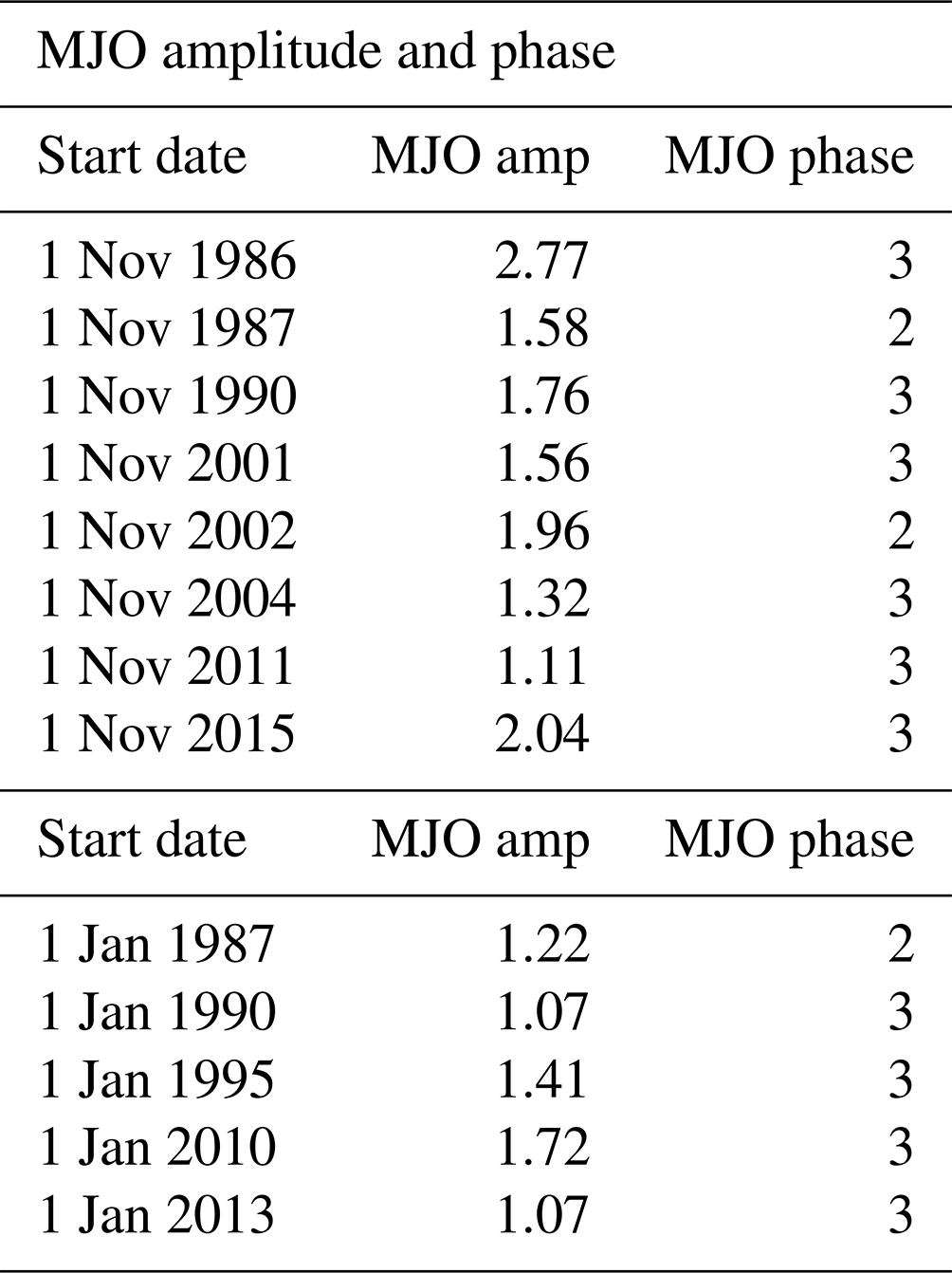
In addition, November and January ensemble reforecasts were made for all years between 1981 and 2016 with the initial dates of 1 November and 1 January. Here the ensemble size is nine, with a control (unperturbed) run and eight perturbed runs. Again the SPPT perturbations were confined to the tropical Indian Ocean. The purpose of these all-year reforecasts is to establish the model reforecast seasonal cycle for the November–December and January–February periods. Table 1 summarizes the MJO and all-year reforecasts, while Table 2 gives the MJO amplitude and phase present on each initial date listed in Table 1. Although these dates span a variety of phases of the El-Niño–Southern Oscillation (ENSO), we do not use a sufficient number of start dates to sample well the different ENSO phases separately.

Table 1 Summary of the model runs performed for this study for the November start dates (left) and the 1 January start dates (right).

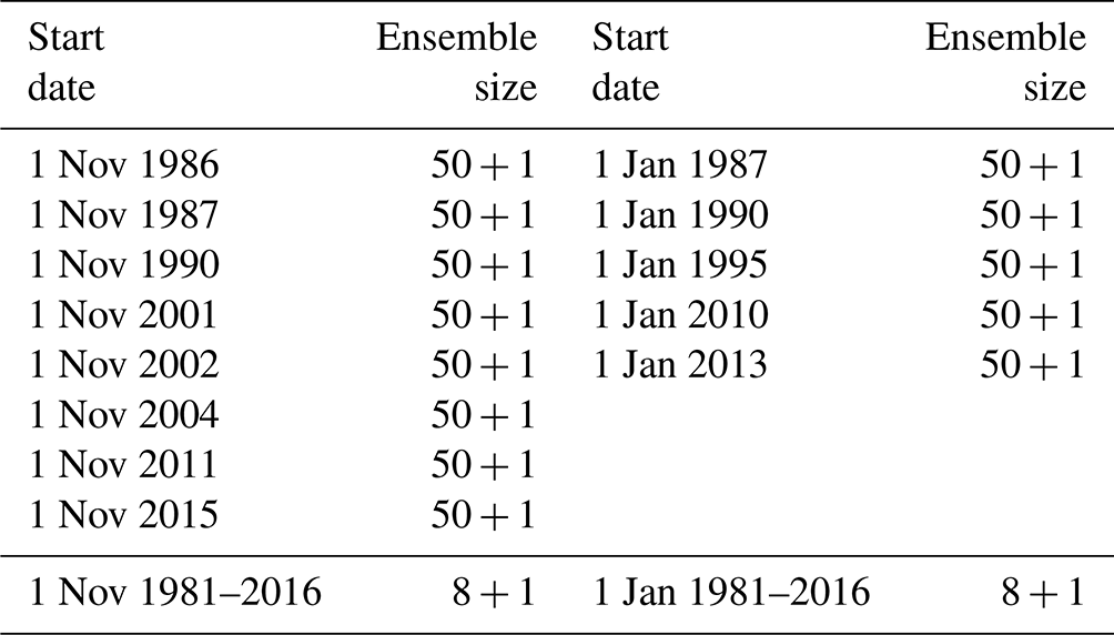
Table 2 Values of MJO amplitude and phase for the initial date of each reforecast ensemble.

2.3 Data and diagnostics

The output of the 60 d forecasts includes the fields of temperature T, geopotential height Z, horizontal winds (u,v) and vertical pressure velocity ω at 12 pressure levels: 1000, 925, 850, 700, 600, 500, 400, 300, 250, 200, 100 and 50 hPa. These fields were available twice daily on an N80 Gaussian (320^∘ × 160^∘) long × lat grid.

The diabatic heating was computed as a residual in the thermodynamic equation, with a resolution equivalent to T159 in spherical harmonic space, following the algorithm described in Swenson and Straus (2021). While the output of the algorithm yields the heating in watts per square meter (W m⁻²) integrated over three layers – 1000–850, 850–400 and 400–50 hPa – in this paper we present diagnostics from both the midlevel (850–400 hPa) heating Q_mid and the full vertical integral heating Q spanning 1000–50 hPa. The daily mean diabatic heating from the ERA5 reanalysis (Hersbach et al., 2020) was computed from the same fields, sampled four times per day, for the Novembers of the 8 years listed in Table 1.

The Rossby wave source was computed following the prescription of Sardeshmukh and Hoskins (1988) as

$$\begin{array}{}\text{(1)}& S=-\mathbf{\nabla }\cdot \left({\mathit{v}}_{\mathit{\chi }}{\mathit{\zeta }}_{\mathrm{a}}\right)=-{\mathit{\zeta }}_{\mathrm{a}}\mathbf{\nabla }\cdot {\mathit{v}}_{\mathit{\chi }}-\left({\mathit{v}}_{\mathit{\chi }}\cdot \mathbf{\nabla }\right){\mathit{\zeta }}_{\mathrm{a}},\end{array}$$

where ${\mathit{\zeta }}_{\mathrm{a}}=f+\mathit{\zeta }$ is the absolute vorticity and the vector v_χ the divergent component of the horizontal flow vector. In other words, S is the sum of the stretching term (vorticity times divergence) and the advection of vorticity by the divergent flow. We shall attempt to diagnose the contribution of each term in Sect. 3 and the Appendix.

In order to compute S, we made use of the following transforms between the Gaussian grid and spherical harmonic (spectral) representations:

$$\begin{array}{}\text{(2)}& {\displaystyle }(u,v)\to (\widehat{D},\widehat{V}),\text{(3)}& {\displaystyle }(\widehat{D},\widehat{V})\to (u,v),\text{(4)}& {\displaystyle }\widehat{F}\to F.\end{array}$$

Here (u,v) are the horizontal components of any vector on the grid, $(\widehat{D},\widehat{V})$ are the corresponding divergence and curl in spectral representation, F is the grid point representation of any scalar field, and $\widehat{F}$ is its representation in spectral space. Applying transform Eq. (2) to the horizontal flow vector gives the ordinary divergence and vorticity in spectral space; transform Eq. (4) then yields the relative vorticity ζ. To obtain the vector v_χ we apply transform Eq. (3) using the spectral divergence $\widehat{D}$ obtained from the horizontal winds but setting $\widehat{V}=\mathrm{0}$. Finally we use Eq. (2) on the vector (u_χζ_a,v_χζ_a) to obtain the corresponding divergence $\widehat{S}=\widehat{D}$ in spectral space, followed by a transform back to S. In applying this last transform, only spectral components corresponding to T21 were retained, and the final field was averaged over 2 d blocks.

In order to consider the source outside the deep tropics (where the background easterlies would suppress a stationary wave response) and in the vicinity of the subtropical jet, we consider the average source between 15 and 30^∘ N. The final values were divided by $\frac{\mathrm{2}\mathrm{\Omega }}{a}$, where Ω is the angular rotation rate of the earth and a the radius of the earth. The scaled values have units of meters per second (m s⁻¹). The results shown in this paper are robust to changes in the latitude band chosen, both to modest poleward displacement and to widening it by 5^∘.

2.4 Definition of anomalies

The seasonal cycles corresponding to the November and January MJO experiments listed in Table 1 are computed from the corresponding all-year experiments and are characterized by a single climatological parabola in time for each variable and grid point, as in Straus (1983). Deviations in time around this seasonal cycle give the anomalies.

2.5 Metrics of uncertainty

Several metrics of the growth in uncertainty are used in this paper. In all cases what is measured is the uncertainty due solely to the spread of each ensemble with forecast time without any reference to reanalysis or observations.

The internal error variance for a variable F is defined as the average squared difference between the perturbed reforecasts (to which the SPPT scheme has been applied) and the control reforecast for the same initial date. It is denoted as $V_{\mathrm{int}}^{\left(\mathrm{F}\right)}$.

The ensemble error variance is defined as the average of the squared difference between the perturbed reforecasts and the ensemble mean. Its square root is referred to as the ensemble spread. It is denoted as $V_{\mathrm{ens}}^{\left(\mathrm{F}\right)}$.

Finally, the external error variance, denoted by $V_{\mathrm{ext}}^{\left(\mathrm{F}\right)}$, is defined as the average of the squared difference between each reforecast and all the control forecasts from the all-year experiments for the same forecast time.

All error variances depend on forecast time, as well as level, latitude and longitude (or zonal wavenumber). The external error variance gives a simple measure of the saturation level of the internal error variance. This saturation level will depend on time due to the evolution of the seasonal cycle.

To express these definitions in formulae, let the index i denote ensemble member, running from 0 (the control forecast) to N=50, and let F_i,j denote the value of the field F for forecast i (i=0 being the control forecast) for initial condition j. Let 〈F〉_j denote the ensemble mean $\langle F{\rangle }_j=\frac{\mathrm{1}}{N+\mathrm{1}}{\sum }_i{F}_{i.j}$, and let ${\stackrel{\mathrm{̃}}{F}}_k$ denote the field F from the control run for year k of the all-year forecasts, with $\mathrm{1}\le k\le K=\mathrm{36}$.

$$\begin{array}{}\text{(5)}& {\displaystyle }{V}_{\mathrm{int}}^{\left(\mathrm{F}\right)}={\displaystyle \frac{\mathrm{1}}{J}}\sum _j{\displaystyle \frac{\mathrm{1}}{N}}\sum _{i=\mathrm{1}}^N{\left(F_{i,j}-F_{\mathrm{0},j}\right)}^{\mathrm{2}}\text{(6)}& {\displaystyle }{V}_{\mathrm{ens}}^{\mathrm{F}}={\displaystyle \frac{\mathrm{1}}{J}}\sum _j{\displaystyle \frac{\mathrm{1}}{N+\mathrm{1}}}\sum _{i=\mathrm{0}}^N{\left(F_{i,j}-\langle F{\rangle }_j\right)}^{\mathrm{2}}\text{(7)}& {\displaystyle }{V}_{\mathrm{ext}}^{\mathrm{F}}={\displaystyle \frac{\mathrm{1}}{J}}\sum _j{\displaystyle \frac{\mathrm{1}}{N+\mathrm{1}}}\sum _{i=\mathrm{0}}^N{\displaystyle \frac{\mathrm{1}}{K}}\sum _k{\left(F_{i,j}-{\stackrel{\mathrm{̃}}{F}}_k\right)}^{\mathrm{2}}\end{array}$$

Note that the error variances of the kinetic energy are just the sum of the corresponding error variances of the components of the horizontal winds (u,v) divided by 2.

3 Results

3.1 Tropical signal

The daily averaged evolution of vertically integrated diabatic heating anomaly is shown averaged for the 60 d experiments in Fig. 1a. The heating has been averaged over the tropical band (15^∘ S–15^∘ N), over all ensemble members and over all experiments. The eastward propagation of positive heating anomalies near longitude 90^∘ E can be seen for about 8 d, along with robust westward propagation of heating anomalies that appear after 4 d in the central Pacific. The ensemble spread of the heating (also averaged over the tropical band and all experiments) is shown in Fig. 1b. The dominant influence of the SPPT-generated perturbations over the Indian Ocean sector is clear, leading to the largest ensemble spread in this sector. Note that the range of longitudes over which the SPPT scheme is applied is shown with the red vertical lines.

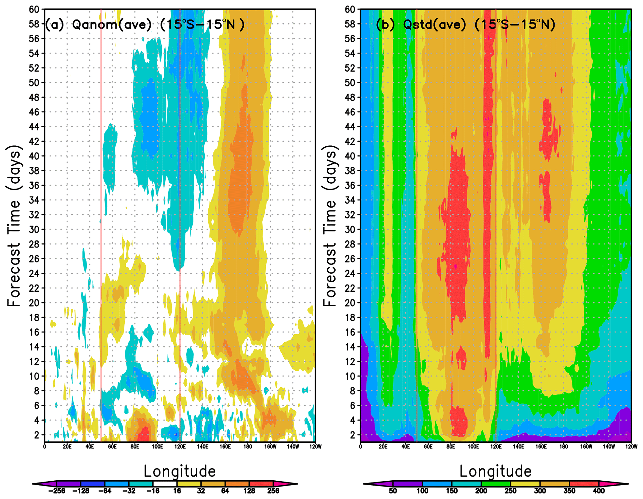
Figure 1 (a) Evolution of the daily mean, ensemble mean anomaly of diabatic heating anomaly Q (averaged 15^∘ S–15^∘ N) for days 1–60 of the 60 d experiments averaged over all experiments. (b) The evolution of the ensemble standard deviation of the daily mean heating (vertically integrated and averaged 15^∘ S–15^∘ N) averaged over all experiments. The abscissa gives the forecast time in days. The red lines indicate the range of longitudes over which the stochastic parametrization was applied. Units are watts per square meter (W m⁻²).

Figure 2 shows the evolution of the ensemble average of the latitudinally averaged RWS, averaged over all experiments for the first 30 forecast days. Figure 2a shows the results for averaging over latitudes 15–30^∘ N, while Fig. 2b shows the results for latitudes 20–35^∘ N. In both cases, coherent eastward propagation is seen over the first 10 d with negative values seen at longitudes 100–140^∘ E. The magnitude of the RWS is larger for the band that extends to 35^∘ N. Beyond forecast day 30, the mean signal in RWS shows little propagation (not shown).

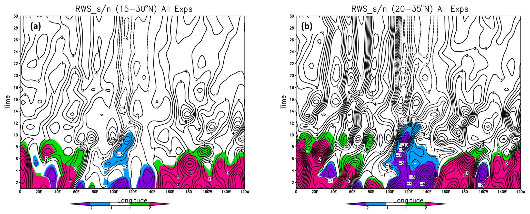
Figure 2 Evolution of the Rossby wave source (S) averaged over all experiments. Time is given in days. The RWS was computed at the equivalent of T21 triangular spectral truncation (see text for details). S was averaged between 15 and 30^∘ N (a) and between 20 and 35^∘ N (b). The color scale gives the ratio of the ensemble mean to ensemble spread. The units of the RWS are meters per second (m s⁻¹).

The colors indicate where the signal-to-noise ratio σ, defined as the ratio of the mean ensemble average to mean ensemble spread, is greater than 1.0 (for positive RWS) or less than −1.0 (for negative RWS). This ratio shows that the propagation of the RWS is coherent (with the magnitude of the signal-to-noise ratio exceeding 1.0) for the first 8 to 10 forecast days.

Figure A2 shows the evolution of the two components of the RWS, the stretching term and the advection of vorticity by the divergent flow (see Eq. 1). While the stretching term generally dominates, the eastward-propagating advection term to the east of the heating maximum is seen to contribute most to the signal at early forecast times.

3.2 Tropical error growth

The daily averaged ensemble spread of vertically integrated heating Q, averaged over all experiments, is shown in Fig. 1b. During the first few days, the heating spread grows substantially between longitudes 90 and 95^∘ in the Indian Ocean, precisely where the mean heating is greatest. The values of the maximum spread decrease after about 6 d, but large spread is seen over a wider area as the uncertainty propagates. (Note for reference that the longitudinal boundaries of the SPPT perturbations are indicated by the faint-red vertical lines in Fig. 1b.)

In order to determine whether the strength of the stochastic perturbations (reflected in the magnitude of the ensemble spread in the Indian Ocean region) is reasonable, we also computed the interannual standard deviation σ_IA of the tropical Q from the ERA5 reanalysis over the 8 years corresponding to the November experiment for the first 30 d. Figure A1 in the Appendix shows the daily evolution of the standard deviation with the same scale as in Fig. 1b. The ERA5 σ_IA is largely confined to the same regions as the model spread: the Indian Ocean region and the west-central Pacific. In the Indian Ocean sector, the model spread in heating has somewhat lower maximum values than σ_IA but extends over a wider area. The model spread is notably less than σ_IA over the Pacific up to forecast day 30.

In order to investigate the scale dependence of the uncertainty of the heating evolution, we calculated the zonal wavenumber spectra of the internal error variance of Q_mid (850–400 hPa) averaged over 2 d blocks and over the tropical belt 15^∘ S–15^∘ N. Figure 3 shows the spectra for the blocks ending on days 2, 4, 6, 10, 20, 40 and 60. The latter is indicated by the red line and can be compared to the external error (a measure of saturation) of the blue line. By day 2, the spectrum is relatively flat down to length scales of about 3000 km, consistent with the variance being forced by perturbations in a narrow longitude range. As time progresses, the variance increases without dramatic change in shape until after day 20, when the larger scales (wavelengths greater than about 3500 km) grow more rapidly than the smaller scales, leading to a steeper variance spectrum by 60 d. If we define the predictability time τ to be the time it takes for the error variance to reach a given fraction of saturation, τ increases with length scale.

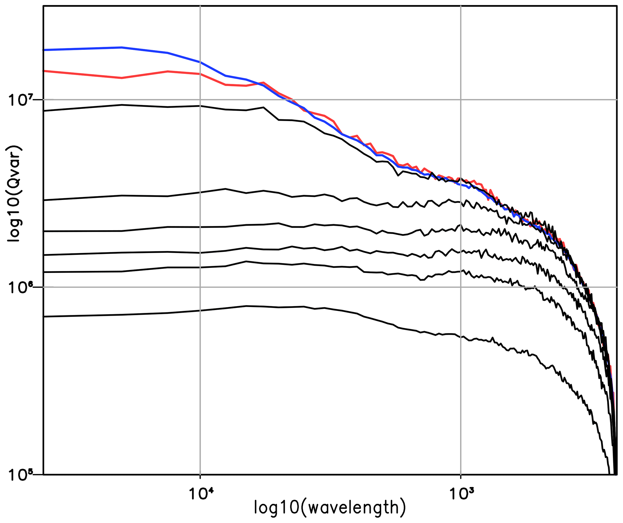
Figure 3 Zonal wavenumber spectra of internal error in midlevel tropical diabatic heating Q_mid for various forecast times. The heating was averaged in 2 d blocks and was averaged over latitudes 15^∘ S–15^∘ N. The six black lines give the spectra (starting at the lowest line) for days 1–2, 3–4, 5–6, 9–10, 18–20 and 39–40. The heating for days 59–60 is shown by the red line and the saturation (external) error by the blue line. Units are log₁₀ (W m⁻²).

To make this more precise, we show the time τ at which the error variance of Q reaches a fraction f_τ of the variance of the external error for f_τ= 0.50, 0.70 and 0.90, as a function of zonal wavenumber in Fig. 4a. The red curves give the results for Q with the solid, dashed and dotted lines, respectively. Prior to calculating the error variances for this plot, we have truncated Q (and the other fields to be shown) to a spherical harmonic T21 representation in order to eliminate excessive noise. τ increases with zonal scale (decreasing wavenumber) for all choices of f_τ, but this is particularly noticeable for f_τ= 0.70 and 0.90. In fact the limit of 0.90 of the external error is never reached for zonal wavenumbers 1 and 2.

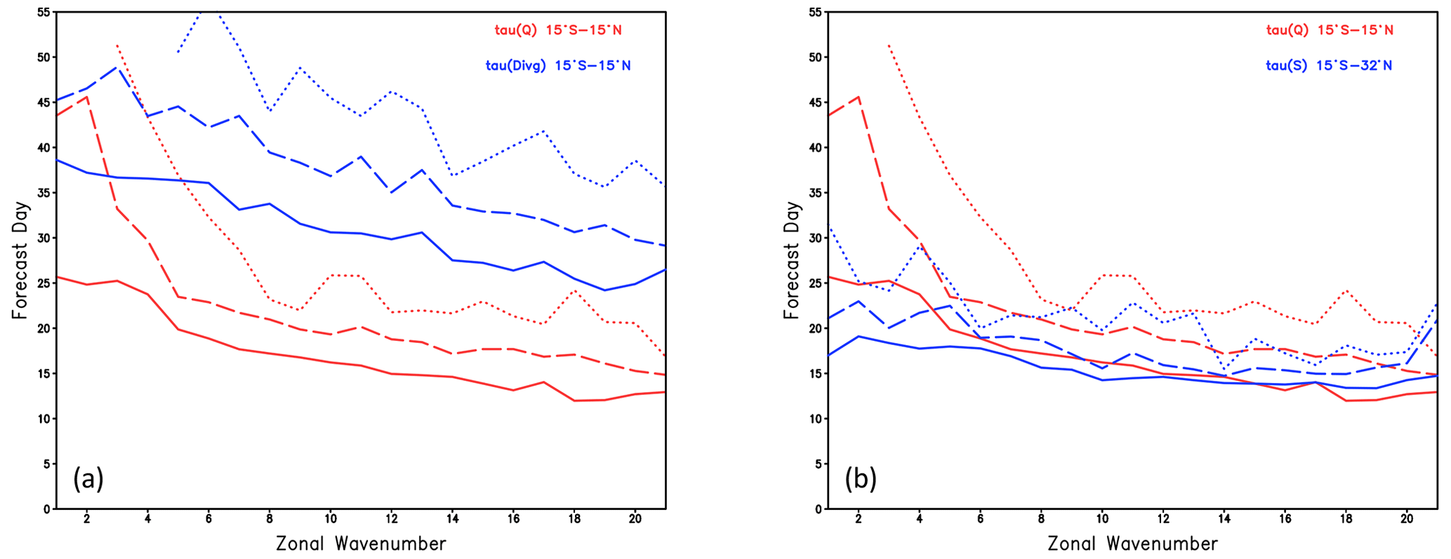
Figure 4 (a) The forecast day τ at which the error variance of heating Q (averaged 15^∘ S–15^∘ N) reaches a fraction f_τ of the external error for f_τ= 0.50, 0.70 and 0.90 shown in solid, dashed and dotted red lines. The blue lines show τ for the 200 hPa divergence averaged over the band 15^∘ S–15^∘ N. (b) τ for the error variance in heating as in (a) along with τ for the Rossby wave source (S) averaged over 15–32^∘ N shown with blue lines.

The predictability times for the T21 representation of the upper-level (200 hPa) divergence are shown in Fig. 4a with the blue curves. These times are notably longer than for the vertically integrated heating. For example, the divergence τ corresponding to f_τ=0.70 is greater than 35 d for the largest scales, compared to 20 d for the heating τ. While this might be taken to indicate high predictability for the extratropical response, the corresponding times for the Rossby wave source, shown with the blue curves in Fig. 4b, are considerably shorter than those for Q. This is especially true for the planetary waves (wavenumbers 1–3) for which the predictability time for the RWS is shorter than that for the heating by about 8 d for f_τ=0.50 and by about 10–20 d for f_τ=0.70. This reflects the sensitivity of the RWS to the subtropical divergent flow and also the subtropical absolute vorticity (as expressed in Eq. 1). The RWS is the sum of the stretching and advection components. Hence the error measures, which are quadratic, will have contributions not only from each component but also from their interaction. Figure A3 shows the total $V_{\mathrm{ens}}^{\left(\mathrm{RWS}\right)}$ as a function of zonal wavenumber and time. The interaction term (labeled NonLin in the figure) was computed by taking the difference between the total error and the stretching and advection components. For zonal wavenumbers greater than about 5, the error in the stretching term dominates, but for larger scales (lower wavenumbers) there is considerable compensation between the stretching and advection terms. The analysis of predictability times for the RWS has not, to our knowledge, been shown before and is an important result regarding the predictability of the extratropical circulation.

3.3 Global error growth

The forecast evolution of the spectra of the internal error variance of kinetic energy (KE) is presented in Fig. 5 for different latitude bands. In the tropics (15^∘ S–15^∘ N; Fig. 5d), the spectra grow without much change in shape between forecast days 3 and 10. Between days 10 and 20 the spectra for smaller scales approach saturation much more quickly than the larger scales do. Wavelengths shorter than about 3500 km are already saturated by day 20, while the larger-scale error variance continues to grow beyond day 40. The times for which the spectra are shown in Fig. 5d (3, 5, 10, 20, 40 and 60 d) are the same as in the other panels (Fig. 5a–c), which show latitude bands of 25–35, 45–55 and 65–75^∘ N, respectively. As one goes to higher latitudes (i.e., from panels c to b to a), the error variance curve for days 3 and 5 continuously moves to lower values, indicating the time it takes for the error to propagate poleward from the tropics. However by day 40, the curves are at about the same level for all latitudes except the 65–75^∘ N band, where the error is less than at other latitudes. The saturation error (estimated by the red curve at day 60) is also less.

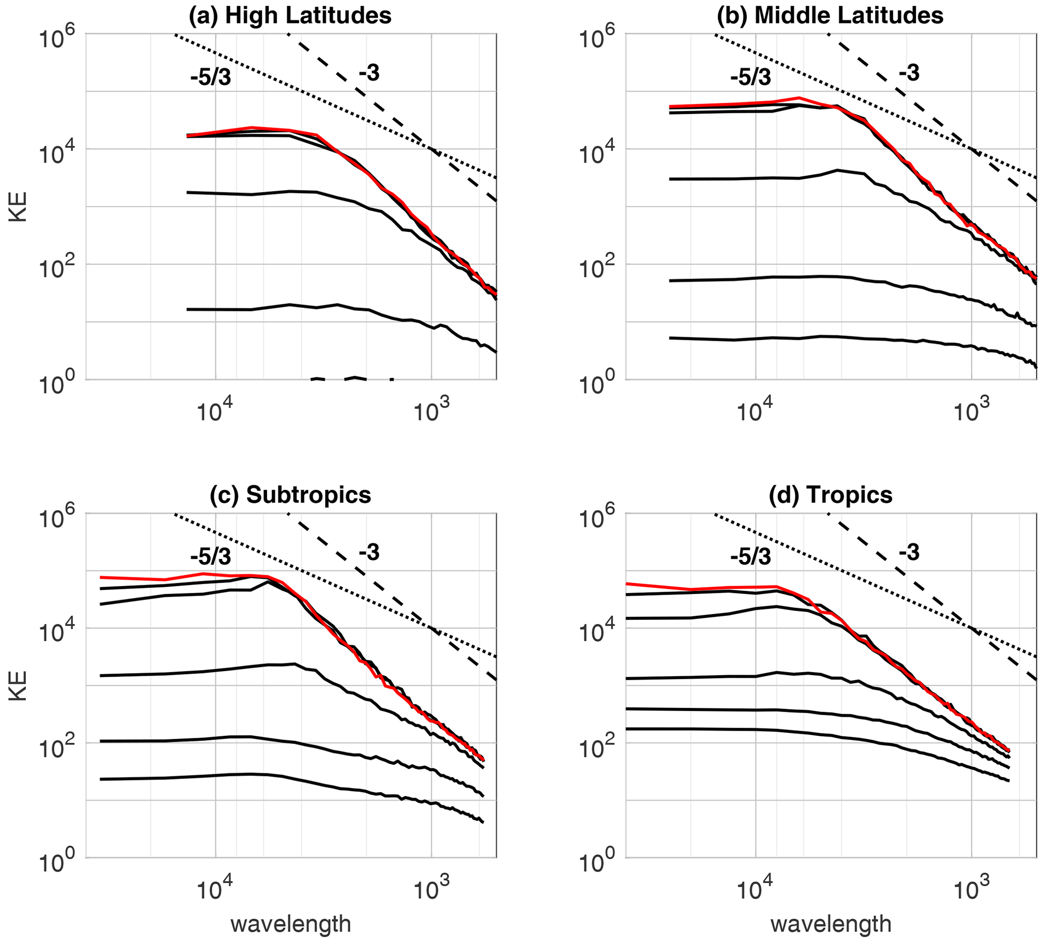
Figure 5 (a) Error variance spectra of 300 hPa kinetic energy, averaged over high latitudes (65–75^∘ N), shown at forecast days 3, 5, 10, 20, 30 and 60 (with the 60 d error shown in red). (b) As in (a) but for middle latitudes (45–55^∘ N). (c) As in (a) but for the subtropics (25–35^∘ N). (d) As in (a) but for the tropics (15^∘ S–15^∘ N). Units are log₁₀ (m² s⁻²). Reference spectral slopes corresponding to a $k^{-\mathrm{5}/\mathrm{3}}$ and k⁻³ dependence are indicated.

To get a sense of how the errors spread geographically, we present maps of the ensemble spread of the meridional wind in Fig. 6. The choice of meridional wind was motivated by its close relationship with storm tracks and circumpolar wave guides (Branstator and Teng, 2017). Much of the tropics outside of the Indian Ocean region is nearly error-free even at day 6. By day 10, substantial error has already appeared in the extratropics, particularly in the storm-track regions, and by day 16 the extratropical spread has almost saturated. By day 30 the spread in the extratropics has essentially reached its saturation value since it does not increase for longer lead times (not shown).

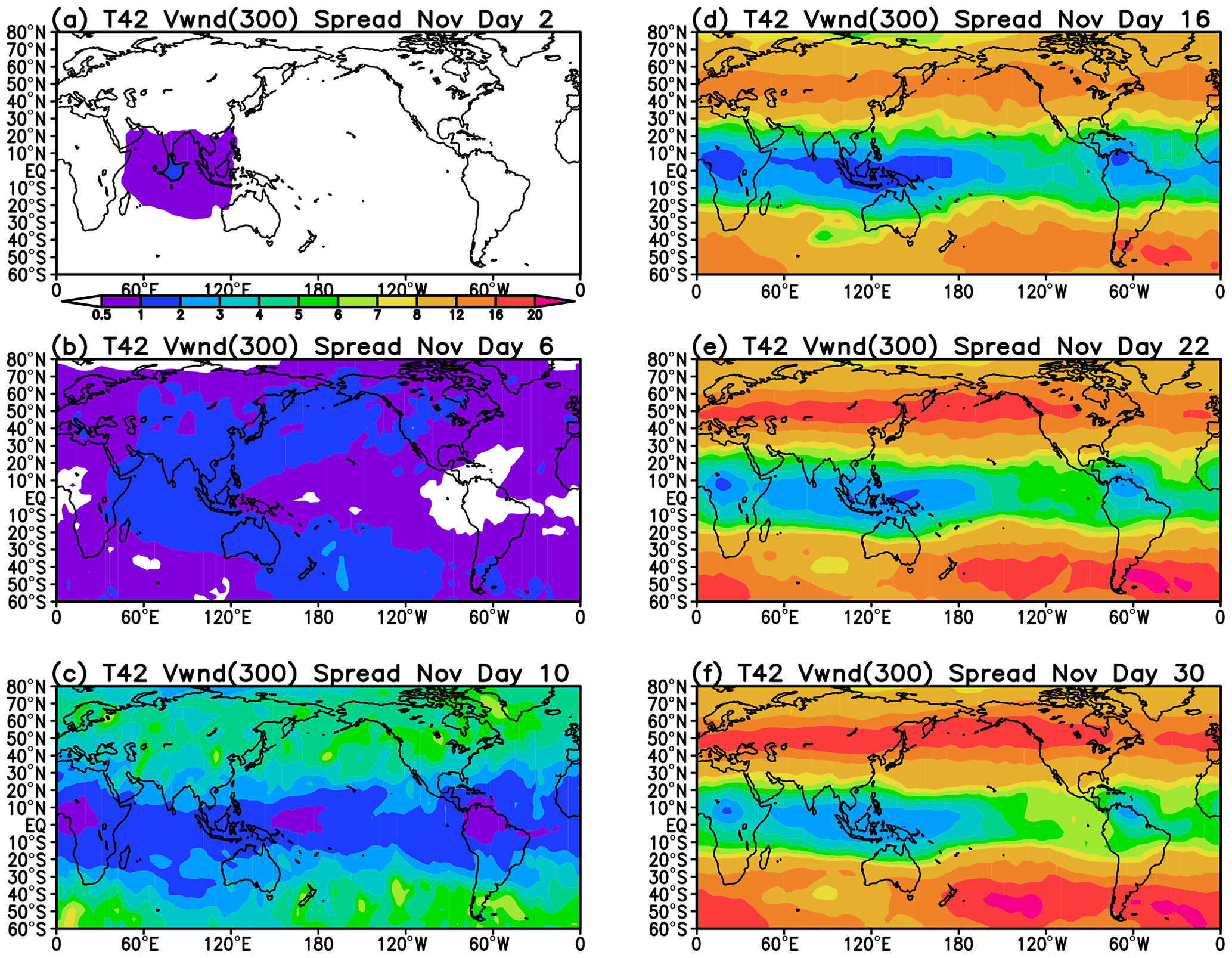
Figure 6 Ensemble spread of meridional wind v at 300 hPa for forecast days 2, 6, 10, 16, 22 and 30. Units are meters per second (m s⁻¹).

3.4 Error propagation through the stratosphere

Since the stratosphere plays a role in the teleconnections from the tropics as a modulator for extratropical long-range forecasts (e.g., Domeisen et al., 2015), we evaluate the role of the stratosphere in error propagation. Since the polar vortex tends to form in middle to late winter (Balwin and Holton, 1988), we present results for the November and January reforecasts separately. The ensemble error variance of the zonal wind u was integrated over the polar cap (60–90^∘ N), and the contributions to the zonal mean error variance from errors in the zonal flow and zonal wavenumbers m=1 to m=3 were computed. The corresponding spread (square root of the variance) is shown in Fig. 7a and b for the November reforecasts and Fig. 7c and d for January reforecasts at levels from 1000–50 hPa. Some evidence for the downward propagation of errors (in the form of ensemble spread increasing from the top, i.e., from 50 hPa) from the stratosphere appears during the last 10 d of the November experiments and slightly earlier in the January initializations in both the zonal mean and planetary wave contributions.

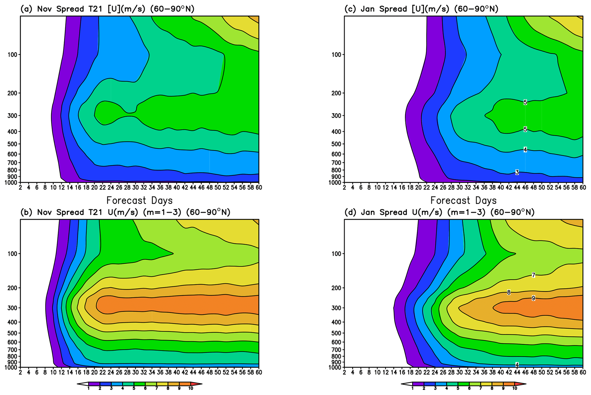
Figure 7 Ensemble spread of the zonal wind u, averaged between 60–90^∘ N for all levels (1000–50 hPa). The spread of the zonal-mean wind [u] is shown in panels (a) and (c) and the spread due to zonal wavenumber 1–3 in panels (b) and (d). The average spread over all November experiments is shown in panels (a) and (b) and over all January experiments in panels (c) and (d). Units are meters per second (m s⁻¹).

The upward propagation of the wave activity from the upper troposphere into the stratosphere, as measured by the vertical component of the Eliassen–Palm flux, is proportional to the zonal mean of the meridional eddy heat flux. Thus we would expect that if the spread in the tropospheric planetary wave activity is responsible for the growing ensemble error in the stratosphere, we should see evidence for this in the spread in the heat flux, especially in the contribution from zonal wavenumbers $m=\mathrm{1}-\mathrm{3}$. Figure 8 shows this heat flux as a function of time and pressure level for both November and January experiments. For the November experiments, enhanced spread in the eddy heat flux is seen by day 30, and by day 40 this spread has grown in the stratosphere. This occurs even earlier (by 10 d) in the January experiments, likely due to the stronger wave flux into the stratosphere and hence a stronger upward coupling. For the November experiments (Fig. 8a), the spread increase in the upper troposphere is seen slightly prior to its increase in the stratosphere, although for the January experiments the increased spread in the troposphere and stratosphere tends to occur nearly simultaneously.

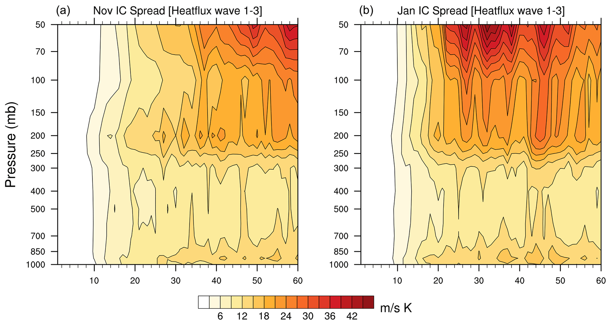
Figure 8 Ensemble spread for meridional eddy heat flux (summed over zonal wavenumbers 1 to 3) averaged between 40–80^∘ N for November (a) and January (b) experiments. Units are meters per second Kelvin (m s⁻¹ K).

In order to better understand the longitudinal dependence of the upward error growth, the geographical distribution of the planetary wave heat flux at 50 hPa is described in Fig. 9. This figure shows both the ensemble mean eddy heat flux due to $m=\mathrm{1}-\mathrm{3}$ and the ensemble spread, whose zonal mean is depicted in Fig. 8a and b. The four rows give pentad time averages for pentads 1, 3, 5 and 7. The heat flux itself is largely confined to the North Pacific in the ensemble mean, which is the region of upward propagation of planetary waves from the troposphere into the stratosphere in the MJO teleconnections (Schwartz and Garfinkel, 2020), but other high-latitude regions contribute substantially to the spread. This is true particularly for the January experiments (columns 3 and 4), in which large values of the spread are seen over the entire belt around 60^∘ N by pentad 5 (forecast days 21–25). The analysis of geopotential height spread at 500 hPa in the North Pacific sector (not shown) gives similar results.

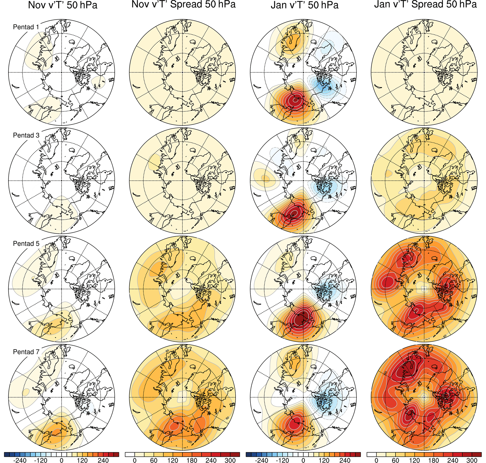
Figure 9 Geographical distribution of the planetary wave contribution to the zonal mean ensemble average and ensemble spread of meridional eddy heat flux at 50 hPa. The ensemble average is shown in columns 1 and 3 and the ensemble spread in columns 2 and 4 (as labeled). Rows 1–4 show averages over days 1–5, 11–15, 21–25 and 31–35, respectively. November experiments are given in columns 1 and 2 and January results in columns 3 and 4. Contour interval is 30 m s⁻¹ K.

4 Discussion

The evolution of tropical heating, averaged over all forecasts, does show the expected distinct eastward propagation for the first 10 d or so. The Rossby wave source shown in Fig. 2 shows a corresponding propagating signal over the broad Indian Ocean region for the first 10 d. While the initial conditions used in these experiments included various phases of ENSO, the small sample size (only 13 distinct initial dates) precludes any meaningful analysis of the dependence of MJO heating on ENSO.

The evolution of the average of the ensemble spread in vertically integrated heating (ΔQ) shown in Fig. 1d shows clearly that the within-ensemble variability induced by the application of the regionally confined SPPT scheme remains mostly confined to that region (50–120^∘ E) for the first 10 d or so. This is also true for the tropical meridional wind spread (Fig. 6) for the first 6 d. By day 10 the perturbations in midlatitudes cover all longitudes. The early confinement of the errors to the tropics suggests that the evolution of the tropical heating and circulation uncertainties would be different had the SPPT scheme been applied throughout the tropical belt. Whether this difference would strongly affect the growth of uncertainty in the extratropics is hard to assess directly from these experiments.

Consistent with the tropical ΔQ remaining somewhat regionally confined, its spectrum is relatively flat over a range of scales for the first 20 d or so (Fig. 3), with the error growth similar for different scales. However, after day 20 scales of less than a few thousand kilometers approach saturation, while the largest scales remain far from saturation. Here the saturation spectrum (given by the blue line) has become steeper, with the largest scales having the greatest variance.

The corresponding predictability times τ, shown in Fig. 4, reveal an interesting result: the upper-level tropical divergence, largely forced by the tropical heating, is far more predictable than the heating, with the largest scales reaching 0.50 (0.70) of their saturation level only near day 40 (50). Clearly the upper-level divergence is relatively insensitive to the details of the heating. A naive interpretation of the tropical divergence as the main forcing function for the extratropics would indicate long-range predictability related to the MJO. However, the predictability times for the Rossby wave source S are considerably shorter: the largest scales reach 0.50 (0.70) of saturation already at around 20 (30) d. This is understandable since S is influenced not only by tropical and subtropical divergence but also by the meridional gradient of the jet. The dominance of the stretching term for moderate scales shown in Fig. A3 is consistent with strong upper-level divergence associated with baroclinic disturbances near the Pacific jet, as expressed by an increase in frequency of warm conveyor belt outflows (Quinting et al., 2023) and also by the behavior of the longitude–time plots of the stretching term that show very consistent eastward propagation (not shown).

Thus we can conclude that one path by which midlatitude and subtropical variability may affect the response to tropical forcing is by changing the effective source for that response. Nevertheless, predictability times for S of 20–30 d are long enough to justify the approach of, for example, Matthews et al. (2004) in using stationary wave concepts to describe the extratropical response to the MJO.

The slopes of the saturation (or background) kinetic energy spectra presented in Fig. 5 are compared to those corresponding to a dimensional wavenumber dependence of k⁻³ and to a dependence of $k^{-\mathrm{5}/\mathrm{3}}$ as indicated by the dashed and solid lines in the figure. (The dimensional wavenumber $k=\frac{\mathrm{2}\mathit{\pi }}{\mathit{\lambda }}$ with λ being wavelength.) A slope corresponding to a k⁻³ dependence is evidence of the dominance of rotational flow, while a $k^{-\mathrm{5}/\mathrm{3}}$ dependence is associated with the dominance of convection and gravity waves and in general divergent flow (Charney, 1971; Sun et al., 2017; Zagar et al., 2017; Li et al., 2023).

Our tropical saturation spectrum, showing a k⁻³ dependence, is in distinct contrast to that of Judt (2020) (their Fig. 5), which shows a slope roughly corresponding to a $k^{-\mathrm{5}/\mathrm{3}}$ dependence, indicative of the dominance of convection and divergent flow. In midlatitudes, the background spectrum of Judt (2020) also shows a transition from a k⁻³ to a $k^{-\mathrm{5}/\mathrm{3}}$ dependence at several hundred kilometers, a transition our results are unable to resolve. These differences are due to the model resolution and dynamics, as J uses 4 km horizontal resolution and storm-resolving simulations without convective parameterizations, while the IFS model used here has a resolution of 36 km and makes use of parameterizations for unresolved processes. Similar to the spectra shown in Zhang et al. (2019) (their Fig. 6), the midlatitude error growth is rapid between days 5 and 10, while the continued error growth for the largest scales at later times is similar to that reported in Selz (2019) in their Fig. 4, noting that the spectra are plotted differently.

The growth of uncertainty in the stratospheric circulation, as seen in Fig. 7, is forced by the upward propagation of the planetary wave meridional flux of sensible heat (which is the dominant term in the vertical component of the Eliassen–Palm flux), shown in Fig. 8. This uncertainty then propagates downward into the upper and middle troposphere. While most of the upper-tropospheric sensible heat flux is due to planetary wave disturbances in the Pacific, its uncertainty in the North Atlantic and Asian sectors are also large, especially for the January experiments (Fig. 9). This downward propagation is potentially linked to wave–mean flow interaction which acts to bring anomalies in, e.g., wind and temperature to the lower stratosphere. The planetary wave error in the upper troposphere (300 hPa) for November reaches a maximum 20 d earlier than the error at 50 hPa does, hinting at a tropospheric forcing of the stratospheric spread.

The stratospheric descent of error seen in Fig. 7 occurs towards the end of the experiments, consistent with the tropospherically forced uncertainty being modulated by the stratospheric circulation (Domeisen et al., 2020b). This descent is seen about 10 d later in the reforecast period for the November experiments than for the January experiments. One factor contributing to this difference is the seasonality of the anomalies of height in the Pacific during phase 3 of the MJO (Wang et al., 2023), which leads to a greater upward component of Eliassen–Palm flux seen for the January experiments in Fig. 9. Another factor is likely to be the lack of a fully formed stratospheric vortex during November so that the establishment of a wave guide for vertically propagating Rossby waves is delayed. (It was not possible to verify this since data were retained only up to 50 hPa.) Note however that separating the effects of the MJO from those of ENSO and other conditions such as stratospheric sudden warmings is quite difficult (Domeisen et al., 2019).

5 Conclusions

The suite of ensemble reforecast experiments presented here was explicitly designed to gauge the effect of the intrinsic uncertainty of subgrid motions on the response to the MJO in phases 2 and 3. Each ensemble has all its members initialized identically during an observed MJO event, and they differ from each other only in the realization of the stochastic parameterizations, applied only in the tropical Indo-Pacific region. Thus even though the errors (deviations within the ensemble) spread globally, they are ultimately due to the uncertainty in this region. These subsequent errors in the tropical diabatic heating, tropical upper-level divergence and Rossby wave source indicate the path towards midlatitude uncertainty in the circulation response. We should point out that our results for the evolution of the Rossby wave source and its error growth hold only for MJO phases 2–3. Since the MJO modulates the Pacific storm track (Lee and Lim, 2012), the behavior of the RWS will be different in other phases of the MJO.

Caveats to this study include the dependence on the particular model used (the IFS) and the lack of comparison to experiments in which the perturbations were applied globally, as in the operational extended-range predictions of ECMWF, or in other regions. The IFS parameterizes convection and other subgrid-scale processes, possibly accounting for the difference between the tropical error spectra seen in these experiments (Fig. 5) and those seen in a convection-resolving model (Judt, 2020). Although we have evidence that the perturbations initially confined to the tropical Indo-Pacific region take at least 10 d to propagate to other tropical regions (Fig. 1), we have not conducted parallel experiments in which the error was applied over a broader tropical band. These await future research.

In conclusion we find the following:

• The uncertainty (average ensemble spread) in total vertically integrated heating is roughly the same magnitude as the MJO signal for the first 5 d but overtakes the signal subsequently (Fig. 1).

• The propagation of the full Rossby wave source is quite coherent in space out to 10 d (Fig. 2).

• The uncertainty of tropical heating is highly scale-dependent: the error on planetary scales has not fully saturated even at the end of the 60 d forecasts, while the predictability time corresponding to 50 % (70 %) of saturation in about 25 (45) d. For scales of roughly 1500 km (zonal wavenumbers 18–20), those times are reduced to 15 to 20 d (Figs. 3 and 4).

• While the predictability times for the planetary wave upper-level divergence are longer than those for diabatic heating (40 to 50 d), the full Rossby wave source is less predictable than the heating (planetary wave predictability times of 20 to 30 d). (Fig. 4). However this is long enough to validate the application of stationary-wave theory to the extratropical response, as in Matthews et al. (2004). The analysis of the predictability of the Rossby wave source is new.

• The kinetic energy error spectra show the spread of error from the tropics to the subtropics, midlatitudes and high latitude, with the error at a give time decreasing as latitude increases (Fig. 5).

• The ensemble spread in meridional wind generated over the tropical Indian Ocean amplifies and propagates into the extratropics, reaching a noticeable amplitude in the midlatitude storm tracks after approximately 15 d, after which it amplifies in situ during the following week (Fig. 6).

• The role of the stratosphere in amplifying uncertainty is generally confined to the latter part of the 60 d reforecasts, which is after the ensemble spread in upper-tropospheric heat flux has affected levels above 50 hPa (Figs. 7 and 8).

Appendix A

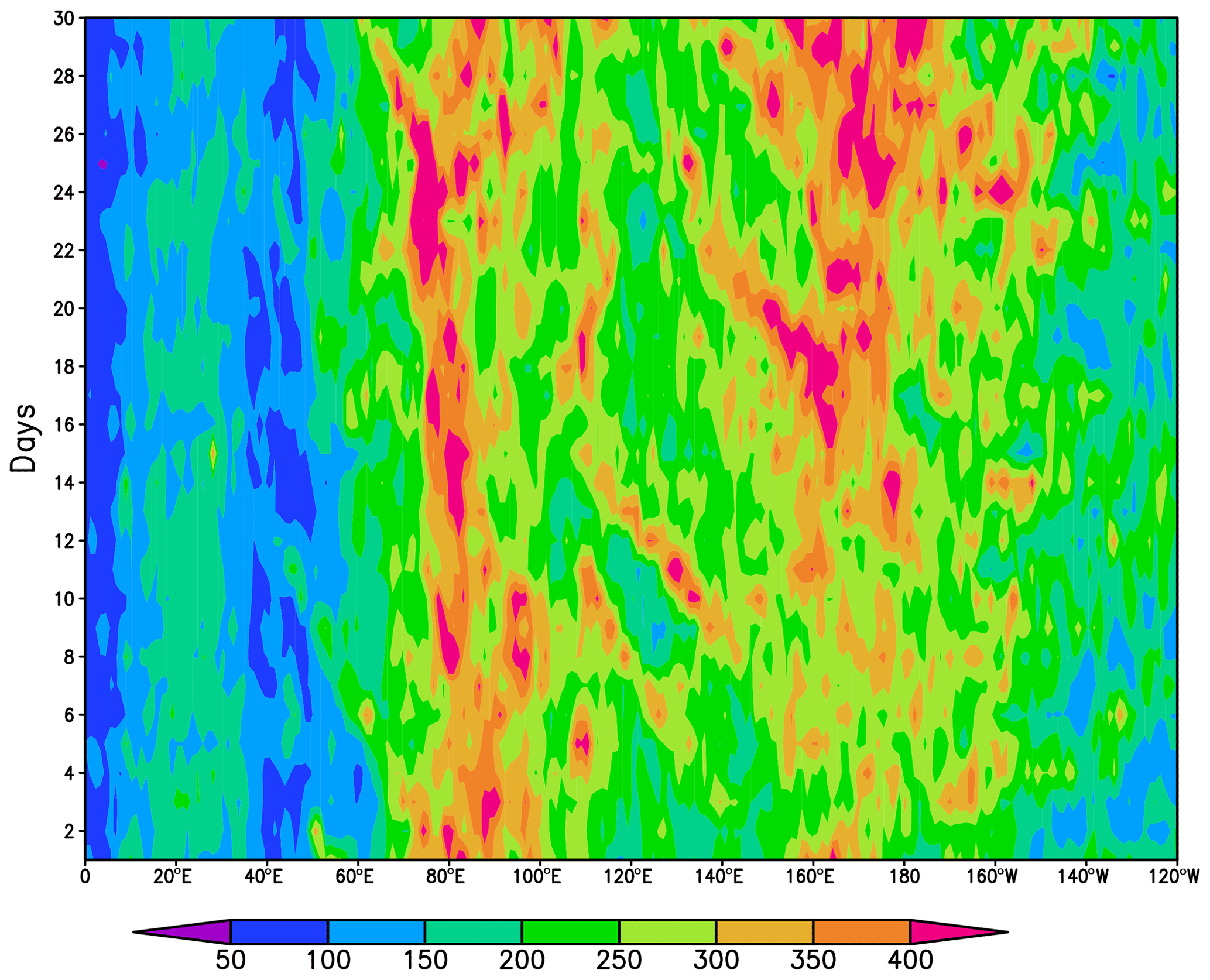
Figure A1 Variance of daily mean, vertically integrated diabatic heating (estimated from ERA5 reanalyses for days 1 to 30 of November) from the 8 years corresponding to the November experiments. See text for details. Units are watts per square meter (W m⁻²).

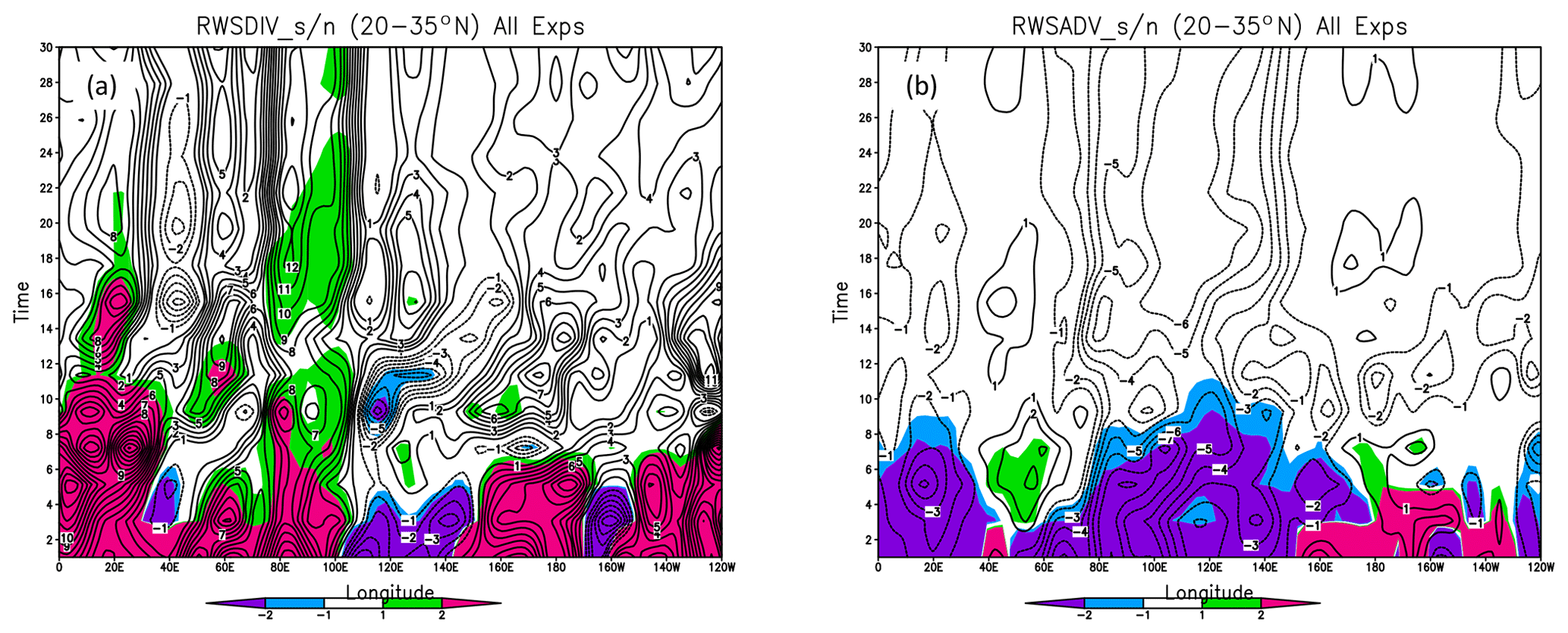
Figure A2 Evolution of the two components of the Rossby wave source (S): (a) the stretching term and (b) the advection term (as in Eq. 1), averaged over all experiments. The terms were computed at the equivalent of T21 triangular spectral truncation (see text for details). S was averaged between 20 and 35^∘ N. The color scale gives the ratio of the ensemble mean to ensemble spread. The units of the RWS are meters per second (m s⁻¹).

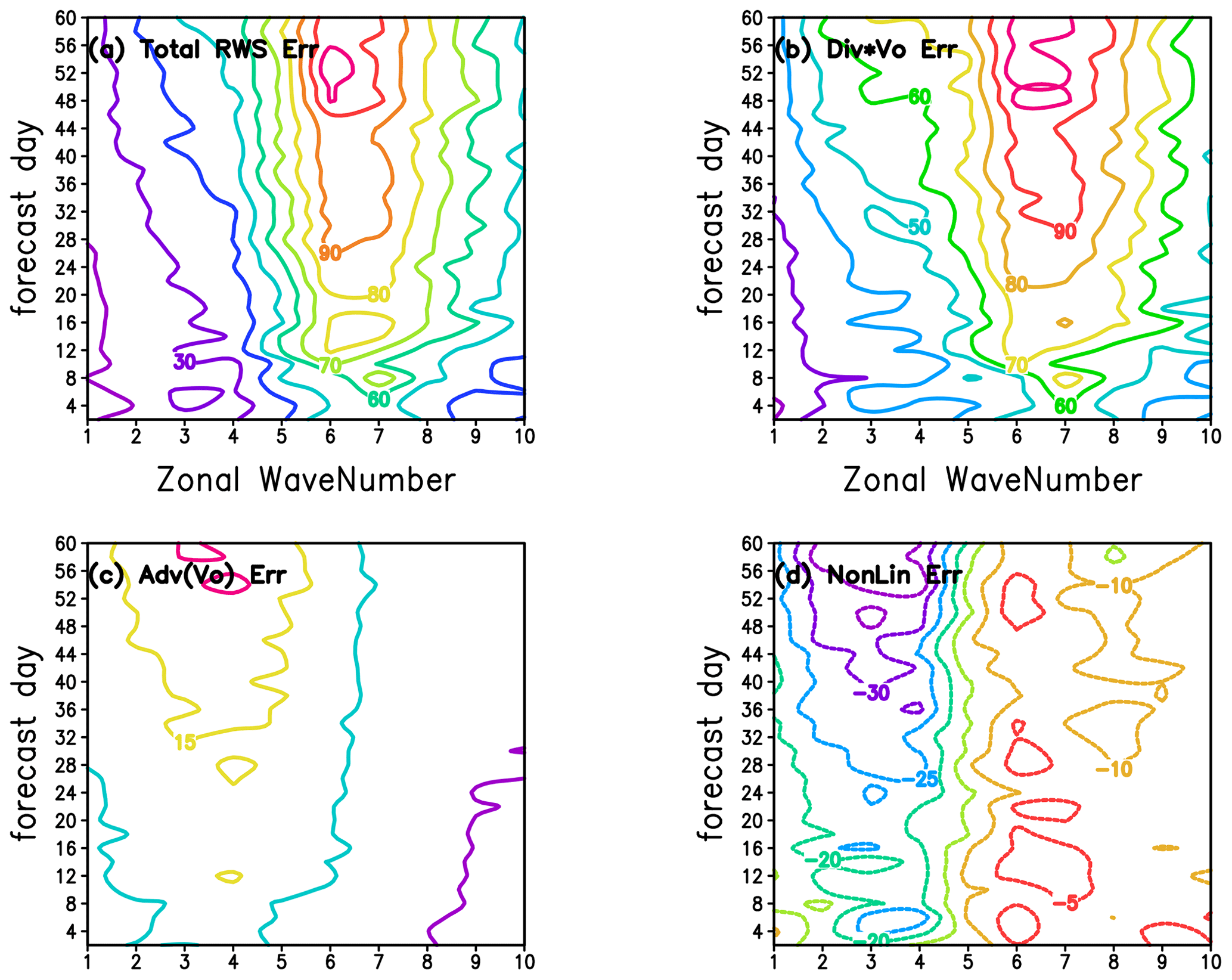
Figure A3 Evolution of the ensemble error of the Rossby wave source (S): (a) the total ensemble error $V_{\mathrm{ens}}^{\left(\mathrm{RWS}\right)}$; (b) the error due to the stretching term alone; (c) the error due to the advection term alone; and (d) the error due to the interaction of the two terms, obtained by subtracting the two contributions (b) and (c) from the total. The errors are averaged over the latitude band 20–35^∘ N. For details see Eq. (1) and the text. All results are averaged over all experiments. The units of the RWS error are (m² s⁻²).