the Creative Commons Attribution 4.0 License.
the Creative Commons Attribution 4.0 License.
 | 07 Dec 2023
Identifying quasi-periodic variability using multivariate empirical mode decomposition: a case of the tropical Pacific
Nour-Eddine Omrani
Noel S. Keenlyside
A variety of statistical tools have been used in climate science to gain a better understanding of the climate system's variability on various temporal and spatial scales. However, these tools are mostly linear, stationary, or both. In this study, we use a recently developed nonlinear and nonstationary multivariate time series analysis tool – multivariate empirical mode decomposition (MEMD). MEMD is a powerful tool for objectively identifying (intrinsic) timescales of variability within a given spatio-temporal system without any timescale pre-selection. Additionally, a red noise significance test is developed to robustly extract quasi-periodic modes of variability. We apply these tools to reanalysis and observational data of the tropical Pacific. This reveals a quasi-periodic variability in the tropical Pacific on timescales ∼ 1.5–4.5 years, which is consistent with El Niño–Southern Oscillation (ENSO) – one of the most prominent quasi-periodic modes of variability in the Earth’s climate system. The approach successfully confirms the well-known out-of-phase relationship of the tropical Pacific mean thermocline depth with sea surface temperature in the eastern tropical Pacific (recharge–discharge process). Furthermore, we find a co-variability between zonal wind stress in the western tropical Pacific and the tropical Pacific mean thermocline depth, which only occurs on the quasi-periodic timescale. MEMD coupled with a red noise test can therefore successfully extract (nonstationary) quasi-periodic variability from the spatio-temporal data and could be used in the future for identifying potential (new) relationships between different variables in the climate system.
- Article
(7088 KB) - Full-text XML
-
Supplement
(7094 KB) - BibTeX
- EndNote


The climate system is a highly complex system consisting of variability across many different timescales (e.g. Baede et al., 2001). Among these, quasi-periodic patterns of variability are important as they can be leveraged for medium-to-long-range predictions (e.g. Mariotti et al., 2018, 2020; L'Heureux et al., 2020). Statistical tools have been particularly helpful in identifying quasi-periodic variability.
The following are typical statistical tools used for exploring the patterns of variability on different temporal and/or spatial scales (Broomhead et al., 1987; Hasselmann, 1988; Penland and Sardeshmukh, 1995; Ghil et al., 2002; Huang et al., 1998; Ghil et al., 2002; Froyland et al., 2021): Fourier transform (FFT), wavelet transform, principal component analysis (PCA), (multi-channel) singular spectrum analysis ((M)SSA), principal oscillation patterns (POPs), linear inverse model (LIM), or even nonlinear Laplacian spectral analysis. However, these methods do not necessarily have a multivariate extension and/or are either stationary, linear, or both. Additionally, some methods, such as (M)SSA, require specification of a window over which quasi-periodic signals are sought, making them somewhat subjective. These can be drawbacks when studying complex, inherently nonlinear, and nonstationary systems, such as the climate system.
Multivariate empirical mode decomposition (MEMD) addresses these drawbacks as it is an analysis tool that is entirely data adaptive and is designed to extract nonlinear and nonstationary signals. MEMD is a generalisation of the empirical mode decomposition (EMD; Huang et al., 1998) to multivariate datasets of more than two time series (Rehman and Mandic, 2010). EMD is a 1-D time series analysis tool that is based on Hilbert transform and takes advantage of the instantaneous frequency, allowing a local extraction of modes of variability. Each mode that the EMD extracts consists of two elements: (1) typical timescale of the mode, i.e. average instantaneous frequency of the mode; and (2) the time series of the mode. Beyond this, MEMD extracts timescales common to all input time series (i.e. synchronises signals) and provides modes (patterns) of variability according to these timescales.
Despite their appeal, MEMD and EMD have hardly been used in climate research. EMD and its 1-D extension ensemble EMD (EEMD; Wu and Huang, 2009) have been used for smoothing, filtering, extracting trends, variability, and testing for red noise distribution of climate data (e.g. Duffy, 2004; Wu et al., 2007; Franzke, 2009; Lee and Ouarda, 2011; Qian et al., 2011; Franzke and Woollings, 2011; Franzke, 2012; Ezer and Corlett, 2012; Ezer et al., 2013; Wang and Ren, 2020). MEMD has only been used for an idealised analysis of atmosphere–ocean coupling strength (Alberti et al., 2021). Moreover, neither MEMD nor EMD has been used for extracting quasi-periodic modes of climate variability.
A major challenge in applying MEMD in climate analysis is that no statistical null hypothesis test for red noise has been developed. When applied to climate data, MEMD can reveal many modes that are consistent with red (or white) noise. In particular, sea surface temperature (SST) exhibits a red spectrum because it represents the integral response of the ocean to stochastic higher-frequency atmospheric (e.g. weather or white noise) variability (e.g. Hasselmann, 1976; Frankignoul and Hasselmann, 1977). However, there are also patterns of quasi-periodic variability (e.g. repeating every 2–8 years) that reflect more complex climate dynamics. To identify such quasi-periodic variability in the climate system, any analysis would first require a significance test that could distinguish this variability from the red noise. In other words, we seek spectral peaks (modes of variability) that pass the red noise threshold (Gilman et al., 1963; Madden and Julian, 1971; Bretherton et al., 1999; see also Sect. 4, Appendix B2).
In this study, we combine the MEMD method with a red noise test (Sects. 3 and 4) to robustly detect quasi-periodic modes of variability. Thus, MEMD becomes well suited for analysing nonlinear and nonstationary climate data. It also has the advantage of objectively detecting intrinsic timescales without pre-selecting and/or filtering for a frequency band (e.g. as in MSSA – multichannel singular spectrum analysis) and without any periodic signal or basis of functions specifications (e.g. as in Fourier transform and wavelet analysis). Since MEMD and (especially) its combination with a red noise test is a new tool in climate science, we test it on a known example of quasi-periodic variability. Namely, we analyse the tropical Pacific atmosphere–ocean variability to extract the El Niño–Southern Oscillation (ENSO). In the future, this tool may be used in other spatio-temporal applications where quasi-periodic variability has not yet been identified.
ENSO is a quasi-periodic phenomenon occurring on (interannual) timescales of 2–8 years (e.g. Philander, 1989; Wang and Fiedler, 2006; Timmermann et al., 2018). ENSO events are characterised by warming tropical Pacific SST during the development of El Niño (warm phase) and cooling of SST afterwards leading into La Niña (cold phase). These events are typically characterised by ocean–atmosphere interaction, whereby atmospheric changes in winds can lead to changes in the distribution of warm and cold waters in the ocean that in turn impact the atmosphere. ENSO exhibits significant nonlinearities, with marked skewness and phase locking to the seasonal cycle (e.g. Stein et al., 2010; Dommenget et al., 2013). It is also nonstationary (e.g. Crespo et al., 2022; Fedorov and Philander, 2000). This complex coupled dynamics is different from red noise and is therefore the focus of the present study.
The paper is structured as follows. Section 2 provides description of data used; Sect. 3 describes the EMD and MEMD implementation (Appendix A provides further details); Sect. 4 provides description of the red noise test (Appendix B provides further details); Sects. 5 and 6 identify modes of variability in the tropical Pacific and explore the physical mechanisms relevant on different timescales. Conclusions are given in Sect. 7.
We focus on the intrinsic variability of the tropical Pacific and analyse monthly mean data of three different variables relevant for atmosphere–ocean exchange: sea surface temperature (SST) from the HadISST observational dataset (Rayner et al., 2003), as well as surface zonal wind stress (τx) and thermocline depth (i.e. the depth of the 20 ∘C isotherm) – both from SODA2 ocean-reanalysis dataset (Carton and Giese, 2008). These three variables are used to assess the ENSO dynamics as these quantities typically play a leading role in the onset and decay of ENSO events and are typically used in the oscillator models that explain ENSO dynamics (see Sect. 6 and e.g. Wang, 2018). The data are analysed in the tropical Pacific (25∘ S–25∘ N, 110∘ E–65∘ W) over the period 1871–2010 for which all datasets are available. Note that surface wind stress and the ocean subsurface data reconstructions in the 19th and early 20th century are less reliable than in the late 20th century due to sparser data coverage; thus, the results presented here are only as accurate as these reconstructions can be (Wittenberg, 2004; Crespo et al., 2022). We use the early record data here to show the nonstationarity and nonlinearity of the tropical Pacific variability over the last ∼ 140 years. The identification of the two main quasi-oscillatory modes (Sect. 5) is also not affected by the inclusion of these data.
The MEMD analysis (Sect. 3) is performed on all fields simultaneously with SST at the highest resolution (1∘ in latitude and longitude), whereas the thermocline depth and τx (both 5∘ resolution in latitude, 9∘ resolution in longitude) have much lower resolution. This gives greater weight to SST data in the analysis and less towards the other variables, such that the mode does not change significantly by adding other variables in the analysis (i.e. results below for the SST are similar whether we use SST alone or together with other fields). This choice is made because we are primarily interested in the quasi-periodic behaviour in SST, since SSTs are used for defining ENSO (e.g. in the Niño3 region – see Table 1). SSTs are also typically smoother than other fields. This is especially true for wind stress, which is strongly affected by the noisy atmospheric variability. This ensures that modes that emerge from MEMD analysis are representative of quasi-periodic variability in SST (and thus ENSO), while the rest of the variables are enslaved to SST variability. The other variables are added to the MEMD input data to describe the climate dynamics involved in the quasi-periodic SST variability, e.g. ENSO (Sect. 6). Note that MEMD can be sensitive to input data; thus, we must carefully consider the input data structure (relevant to a specific study).
Table 1Tropical Pacific regions used for computing time series (see text for details). The rightmost column lists the variables that are averaged over specified regions.
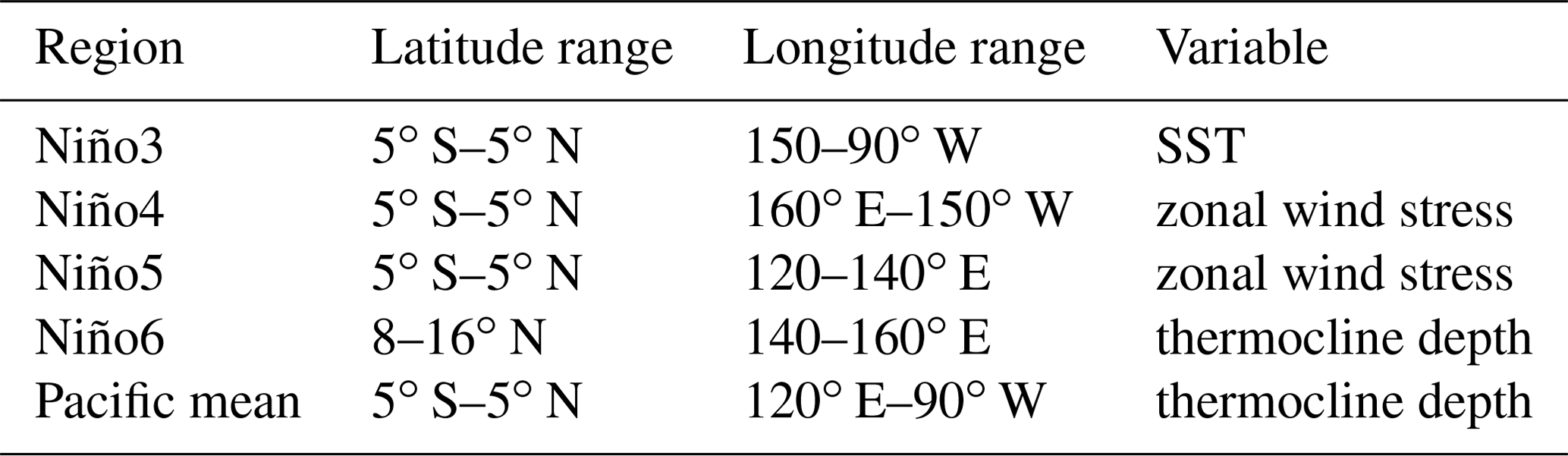
While the SST, thermocline depth, and τx play an important role in the ENSO dynamics, it is specific regions (see Table 1) that have historically been analysed in more detail, for example, in conceptual oscillator models (e.g. Jin, 1997a; Wang, 2018). The time series in the specific regions are thus used to assess if MEMD modes on ENSO timescales are consistent with physics described by conceptual oscillator models (Sect. 6). Additionally, analysing such time series helps with a simpler visualisation of temporal evolution of different variables. Thus, we average τx over Niño4 and Niño5 regions separately, the thermocline depth over the Niño6 region (off-equatorial thermocline depth) and over the tropical Pacific (Pacific mean), and the SST over the Niño3 region (again, see Table 1; see also Fig. 3 in Wang et al., 1999). Note that regional averages (Table 1) are computed after the MEMD analysis is performed (for details see Sect. 3).
Before performing the analysis, we detrend the data and remove their seasonal cycle, which is done the following way (see also, e.g., de la Cámara et al., 2019). First, we calculate 30-year means centred on every 10th year for each individual month. This yields one value for each individual month every 10 years. Then we interpolate between these values (of every 10th year) to obtain yearly time series, again for each individual month. This yields a smooth seasonal cycle that includes a trend and seasonal cycle for every month in the record. Detrended and deseasonalised data are then computed as the difference between the original monthly time series and the smooth trend/seasonal cycle. We do this at every grid point and for every variable separately.
This is done to avoid domination of the seasonal cycle or trend in the statistical analysis below, even though the MEMD can generally extract nonlinear trends by itself. Note that this means that we cannot assess the impact of long-term variability or seasonal cycle on ENSO variability in this study, but the latter may still be present indirectly, as ENSO is phase-locked to the seasonal cycle (e.g. Stein et al., 2010; Wengel et al., 2018).
3.1 MEMD description
We employ MEMD to objectively identify intrinsic modes of variability in nonlinear and nonstationary spatio-temporal data. To understand MEMD, it is easier to first consider the simpler implementation of the 1-D version, empirical mode decomposition (EMD), as outlined by Huang et al. (1998):
- i.
Local minima and maxima of the input (1-D) time series (e.g. see black solid line in Fig. 1) are identified.
- ii.
Envelopes are created by interpolating between subsequent maxima (upper envelope, shown as grey dotted line in Fig. 1) and between subsequent minima (lower envelope, represented by grey dashed line in Fig. 1).
- iii.
An average envelope is obtained by taking the mean of the upper and lower envelopes (depicted by the red solid line in Fig. 1).
- iv.
The average envelope is subtracted from the original time series data.
- v.
The subtracted data, i.e. the original data minus the average envelope, represent the first mode of variability and typically correspond to the highest-frequency signal in the dataset. However, the average envelope can be further analysed.
- vi.
Steps i–vi are repeated on the average envelope until only a trend or residual component remains. This occurs when we can no longer find at least two extrema in the dataset, which is a condition that needs to be satisfied by EMD's modes of variability.
The resulting modes of variability (i.e. the output of the EMD analysis), represented by their respective time series, are known as intrinsic mode functions (IMFs). The timescale of each IMF is characterised by the time lapse between two subsequent extrema, and the mean timescale of an IMF represents the average over all time lapses within its time series.
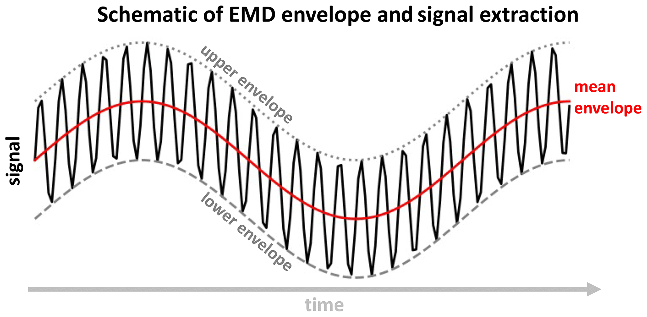
Figure 1Schematic for obtaining the average envelope during the EMD process. The black line shows a simple input signal that is a sum of two sine waves (a low-frequency and a high-frequency wave). Grey dotted and grey dashed lines show the upper and lower envelope, respectively. The red line shows the average envelope, which represents the low frequency of the input signal. If we remove the average envelope from our input data, we obtain the high-frequency signal (e.g. the first mode of EMD).
Additionally, each IMF has to satisfy two criteria: (a) the number of extrema and the number of zero crossings differs at most by one and (b) the mean value of the envelope of the IMF is zero. Note that the procedure from i to iv does not necessarily satisfy (a)–(b) immediately; thus, an additional sifting process (typically iterative) is used, which requires a stopping criteria to ensure the physical meaning of the IMFs. The stopping criteria can be based on the standard deviation of each IMF and on the maximum number of iterations, among others, which set tolerance and confidence limits for the IMF (for details see Huang et al., 1998; Rilling et al., 2003; Huang et al., 2003). Ultimately, this process extracts modes of variability that consist of (1) the typical timescale of the mode and (2) its time series. The modes are automatically ordered from the highest (shortest) in the first mode to lowest (longest) frequency (period) in the last mode. Note that modes that emerge are largely independent with only small correlations between them.
MEMD (Rehman and Mandic, 2010) is a generalisation of the EMD to multivariate datasets of more than two time series (for bivariate and trivariate data separate methods exist; Rilling et al., 2007; Rehman and Mandic, 2010). The method solves a similar problem as in i–vi, but the mean envelope is computed as (Rehman and Mandic, 2010) “an integral of all the envelopes along multiple directions in an N-dimensional space” (i.e. on an N sphere). This is much more complex, but the basic idea remains similar to the 1-D method, and the method retains similar stopping criteria for the sifting process. For further details on and visualisations of the method the reader is referred to Rehman and Mandic (2010) and Alberti et al. (2021).
The MEMD ultimately extracts timescales common to all input time series (i.e. synchronises signals; Rehman and Mandic, 2010) and provides multivariate IMFs (i.e. the outputs of MEMD method) describing those timescales. The timescales of IMFs are then consistent across the input time series – to visualise this, see Supplement Figs. S6–S10, Tables S1–S2, and Sect. S.3 for an idealised example.
As with all statistical methods, it is important to be aware of the drawbacks associated with the (M)EMD (e.g. Stallone et al., 2020). Similar to other time-series-filtering methods, (M)EMD can encounter issues at the edges of the time series, which can result in travelling waves and thus unrealistic peaks in the time series (e.g. Stallone et al., 2020). Another common challenge with (M)EMD is the mixing of modes (see below) where a single genuine mode may be split into multiple modes if inappropriate parameters are chosen (e.g. Huang et al., 1999, 2003; Stallone et al., 2020). However, this issue can also arise when there is no clear timescale separation. To address these challenges, it is crucial to test the physical relevance of the modes of variability identified using (M)EMD and to ensure convergence and stability of the modes through different parameter sweeps that are related to the stopping criteria (see Sect. 3.2). Note that different parameter sweeps may be relevant for different applications.
3.2 MEMD parameter sweep
The code for the MEMD is freely available on GitHub (https://github.com/mariogrune/MEMD-Python- (last access: 1 December 2020); similarly for the EMD discussed above: https://github.com/laszukdawid/PyEMD, last access: 4 December 2023), and the user ultimately only decides about the stopping criteria. These are set to the “fix_h” parameter following Huang et al. (2003), who suggest that limiting iterations yields better-behaved IMFs than other stopping criteria. We limit the number of iterations to 15 (parameter “n_iter” is 15), though other values were tested and a range for “n_iter” around 5–30 yielded similar results, suggesting some convergence for the significant modes of variability (see below).
Note that at higher/lower frequencies we find mode mixing in our MEMD analysis where timescales are not clear (here, this occurs on timescales shorter than about 8 months and longer than about 700 months), as well as with a larger number of iterations. These modes are not detected as different from red noise (see Sects. 4 and 5 for more details). However, the significant modes of variability on interannual timescales that are of interest here are largely unaffected by this (Sect. 5).
3.3 Obtaining modes of variability via MEMD
As mentioned in Sect. 2, we use 3-D data relevant for ENSO dynamics, i.e. (with Lt the length of the time dimension, Ly the length of the latitude dimension, Lx the length of the longitude dimension, and A the selected variable(s)/field(s); bold letters represent two- or three-dimensional arrays) as the basis for the MEMD analysis, which is done the following way.
- i.
First, we remove the smooth trend/seasonal cycle (described above; see also de la Cámara et al., 2019) from A to get a temporal anomaly, A′.
- ii.
We divide data by their standard deviations (σ; done separately for each variable and at each grid point).
- iii.
Since we use more than one variable (i.e. SST, surface wind stress, thermocline depth) in the analysis, we concatenate (denoted with ⊕) the different variables in their spatial dimensions; i.e. we get (with subscripts 1, 2, etc., representing spatial dimensions of the different variables).
- iv.
Then, we reduce the dimensionality by computing spatial patterns (empirical orthogonal functions, EOFs) and their time series (principal components, PCs) via singular value decomposition (SVD).
- v.
Finally, we only retain the first 20 PCs that explain the majority of the variance in the field A′. The PCs are then used as input data for the MEMD algorithm (for further details on the whole procedure see Appendix A).
MEMD analysis identifies 21 IMFs that are ordered by frequency from the highest (IMF 1) to the lowest (IMF 21) with the last 21st mode typically representing a trend, which in our case was already removed (see above). Namely, we find 21 potential intrinsic timescales within the tropical Pacific, i.e. common to all input PCs. This means that we obtain 21 IMFs for each PC time series, i.e. PC, with s the IMF number and m the PC number, where the sth IMF of each PCm has the same timescale (see Table S2). Since we initially obtained PCs via SVD analysis and we thus have corresponding EOF patterns, we can then reconstruct spatio-temporal patterns of variability for each field (i.e. SST, wind stress, and thermocline depth) from PCs and EOFs. The interest here is in the variability on different timescales (i.e. for each (sth) IMF separately, we can perform this reconstruction for each IMF across all 20 PCs/EOFs):
Please recall that input data for MEMD analysis were divided by σ; thus, for the variability of a field in its original units we need to multiply spatio-temporal IMFs by σ.
To compute an index, such as the eastern Pacific SST (Niño3), we can average over a latitude–longitude region (Table 1) from spatio-temporal IMFs (Eq. 1) to obtain time series of, for example, the eastern Pacific SST (Niño3) for each IMF separately – see Figs. S6–S10 for time series of different variables from Table 1 and Table S1 for their timescales. This yields an index for each IMF (e.g. IMFs(SST (Niño3)), with s the IMF number) corresponding to an equivalent index computed from input data (A′). The latter is approximately the same as the sum of indices computed from all IMFs, e.g. .
Once we have computed the IMFs, we need to test if they are statistically significant. The importance of each IMF can be assessed by computing the explained variance of each IMF relative to the input field (e.g. retaining those IMFs that explain more than 0.1 % variance) or through other significance tests (e.g. white noise test; Appendix B1; Wu and Huang, 2004). We develop a test for variability that can be distinguished from red noise, as appropriate for studying climate variability (see Introduction).
The red noise test can be performed in different ways (see also Sect. 5.1): (i) we can choose an index of interest and perform a red noise test on its IMFs (see below; Fig. 2) – this can be used when we are interested in the quasi-oscillatory behaviour of a specific index (e.g. areal average) we constructed or a known climate index we wish to test; (ii) more objectively, we can use IMFs of specific PC time series (e.g. PC1; Fig. S2) – this can be used when we are interested in quasi-oscillatory behaviour of an index that explains a specific amount of variance in a field or region (e.g. tropical Pacific); and (iii) we can test for quasi-periodic variability at each grid point (Sect. 5.1, Fig. 5) – this can be used to identify potential regions of quasi-oscillatory behaviour that have not been identified before. In general, all methods can be used together (as done here) for robustness, but their use will ultimately depend on the specific scientific question.
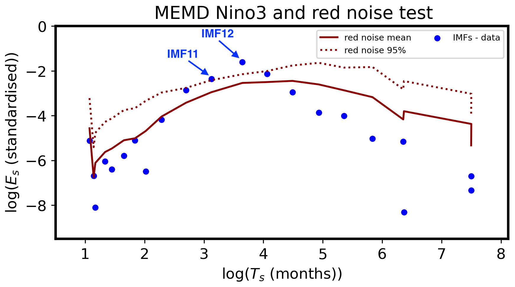
Figure 2The red noise significance test for spatio-temporal IMFs (from MEMD) via SST averaged over the Niño3 region (for details see text and Appendices A and B). Each blue dot represents the average squared amplitude (Es; Eq. B1) and average period (Ts; in months; for periods of IMFs see Table S1) of each IMF that we have identified within our time series/data. The average period is computed from the instantaneous frequency obtained via Hilbert transform (see text under Eq. B4). For visualisation purposes we obtain a natural logarithm of both the average squared amplitude (log e(Es); y axis) and the average period (log e(Ts); x axis) of each IMF and plot them as a scatterplot (blue dots). Note that the logarithms of periods (log e(Ts)) are ordered from the shortest period (highest frequency; IMF 1; leftmost blue dot) to the longest period (trend; IMF 21; rightmost blue dot). The red solid line represents the theoretical red spectrum fit (Eqs. 2 and B7–B9), and the red dotted line represents the one-tailed 95th percentile confidence level (via χ2 test). For further descriptions of the figure see text.
Here, we first test for potential quasi-periodic variability using SST time series that are relevant for (eastern Pacific) ENSO variability, i.e. the eastern Pacific SST (Niño3) from input data and the corresponding eastern Pacific SST (Niño3) from spatio-temporal IMFs (as described in Sect. 3; IMFs (SST (Niño3))). Then, we compute the power spectrum for each timescale/period (i.e. each IMF) by obtaining the average squared amplitude of each (sth) IMF (Es), i.e. (with Lt the length of the time series and j each time step). The average timescale (Ts) of each IMF is computed from the instantaneous frequency using Hilbert transform (see text around Eq. B4 in Appendix B1), which yields similar results to computing the time lapse between two extrema in the time series. Es is then plotted against Ts (here we use their logarithmic values) to yield the power spectrum plot (blue dots in Fig. 2).
The shape of the red noise fit (red solid line in Fig. 2), or rather red noise spectrum for every sth IMF, can be computed from the lag-one autocorrelation of the input data (e.g. eastern Pacific SST (Niño3)) as (see also Gilman et al., 1963; Kolotkov et al., 2016; for full derivation and further discussion see Appendix B)
is a theoretical estimate of the (mean) energy of the red noise of the sth IMF, is frequency, t is time, r is the lag-1 auto-correlation of input data of the eastern Pacific SST (Niño3), and , and subscript s represents the sth IMF of frequency νs (ordered from highest to lowest frequency).
is then scaled so that the variance of the red noise fit is identical to the variance of the spectra computed from the spatio-temporal IMFs (Es; Eq. B9; see also Madden and Julian, 1971; Bretherton et al., 1999). The 95 % confidence curve (red dashed line in Fig. 2) is computed by multiplying the red noise fit by the χ2 statistic for a one-sided p value of 0.05. The number of degrees of freedom for the sth IMF is computed as (for further details see Appendix B2; see also Bretherton et al., 1999; Wu and Huang, 2004; Kolotkov et al., 2016). Note that the same procedure (as described above) can be applied to any other time series/IMFs.
As MEMD in conjunction with a red noise test has not been applied in climate science before, we perform an extensive analysis of the method itself (in addition to an analysis of ENSO dynamics – see below). Then, we compare it to the basic band-pass filtering (fifth-order Butterworth filter) and to Fourier transform analysis to ensure consistency with other methods. Please recall that while other spectral methods often require prior knowledge about the spatial/temporal patterns of interest in order to construct appropriate indices, the MEMD method allows for the objective extraction of significant patterns and modes of variability from data without pre-existing knowledge (see also below and Appendices A and B).
5.1 Significant modes of variability
We identify two significant modes of variability in the eastern Pacific: the 11th IMF (IMF 11) and 12th IMF (IMF 12) (shown with blue arrows in Fig. 2) with average timescales of ∼ 23 and ∼ 39 months (∼ 2–3 years; see also Table S1), respectively. Their timescales fall well within the typical ENSO timescale range (2–8 years), as can be identified via a typical power spectrum analysis (Appendix B2, Fig. B3). These timescales (with their uncertainty ranges; see below) are consistent with previously identified quasi-biennial (QB; ∼ 2 years) and low-frequency/quasi-quadrennial (LF/QQ; ∼ 4 years) ENSO modes (e.g. Jiang et al., 1995; Allan, 2000; Kim et al., 2003; Keenlyside et al., 2007; Bejarano and Jin, 2008; Jajcay et al., 2018; Froyland et al., 2021).
The quasi-periodic mode of variability with a 39-month average period (IMF 12) is more statistically significant (than IMF 11). This can be seen in different ways. First, considering the Niño3 index (i.e. the eastern Pacific SST in the Niño3 region), IMF 11 (blue dot) lies only slightly above the 95 % red noise threshold (red dashed line), whereas IMF 12 lies well above the threshold (Fig. 2). Second, considering the PC1's IMFs (i.e. before we do spatio-temporal reconstruction of IMF data; Fig. S2), only IMF 12 is found to be significant, despite the generally good agreement between the Niño3 index and PC1 of the tropical Pacific SST (e.g. Ashok et al., 2007). Finally, we can perform a red noise test on each grid point of the tropical Pacific (similarly as for specific time series shown above) and plot the spatial structure of SST together with the significance test (Sect. 6, Figs. 5, S3). This shows that none of the grid points of spatio-temporal IMF 11 pass the red noise threshold (Fig. S3), but many grid points of the spatio-temporal IMF 12 are significant (not shaded in grey in Fig. 5).
Nevertheless, even though IMF 11 is marginally statistically significant, the MEMD analysis suggests that there may be two quasi-periodic modes of interannual SST variability in the tropical Pacific region. This agrees with previous results that have identified two statistically significant modes of variability with specific frequencies and distinguished by their dynamics. Note that we also find that the two modes of variability are well separated (in terms of timescale) from the other modes and from each other, as shown by Fig. 2. This ensures no mode mixing on the quasi-periodic timescales.
On longer timescales, we do not find any behaviour that would be discernible from red noise, suggesting that the lower-frequency range of ENSO (timescales longer than ∼ 4.5 years) (e.g. Allan, 2000; Jajcay et al., 2018) is better represented by red noise. Recall, however, that any potential oscillatory behaviour on timescales longer than 30 years was removed via detrending. Similarly, we do not find any quasi-periodic modes of variability on shorter timescales. Also, on these longer (> 700 months) and shorter (< 8 months) timescales we find some mode mixing. This is likely a consequence of inputting several different variables (i.e. SST, τx, thermocline depth) into the MEMD algorithm, where each variable can have different timescales represented. For example, wind stress can be much noisier than SST (or different parts of the tropical Pacific have different variabilities) and can thus lead to identification of several high-frequency modes of variability, resulting in mode mixing (see somewhat overlapping blue dots in Fig. 2).
5.2 Time series of significant modes of variability
Above we have established that the Niño3 index in the tropical Pacific exhibits two quasi-periodic modes of variability with average periods ∼ 2–3 years (via MEMD analysis). We now analyse the associated time series of the two IMFs (IMF 11 and IMF 12) and compare them with a band-pass-filtered (16–53 months) Niño3 index (Fig. 3).
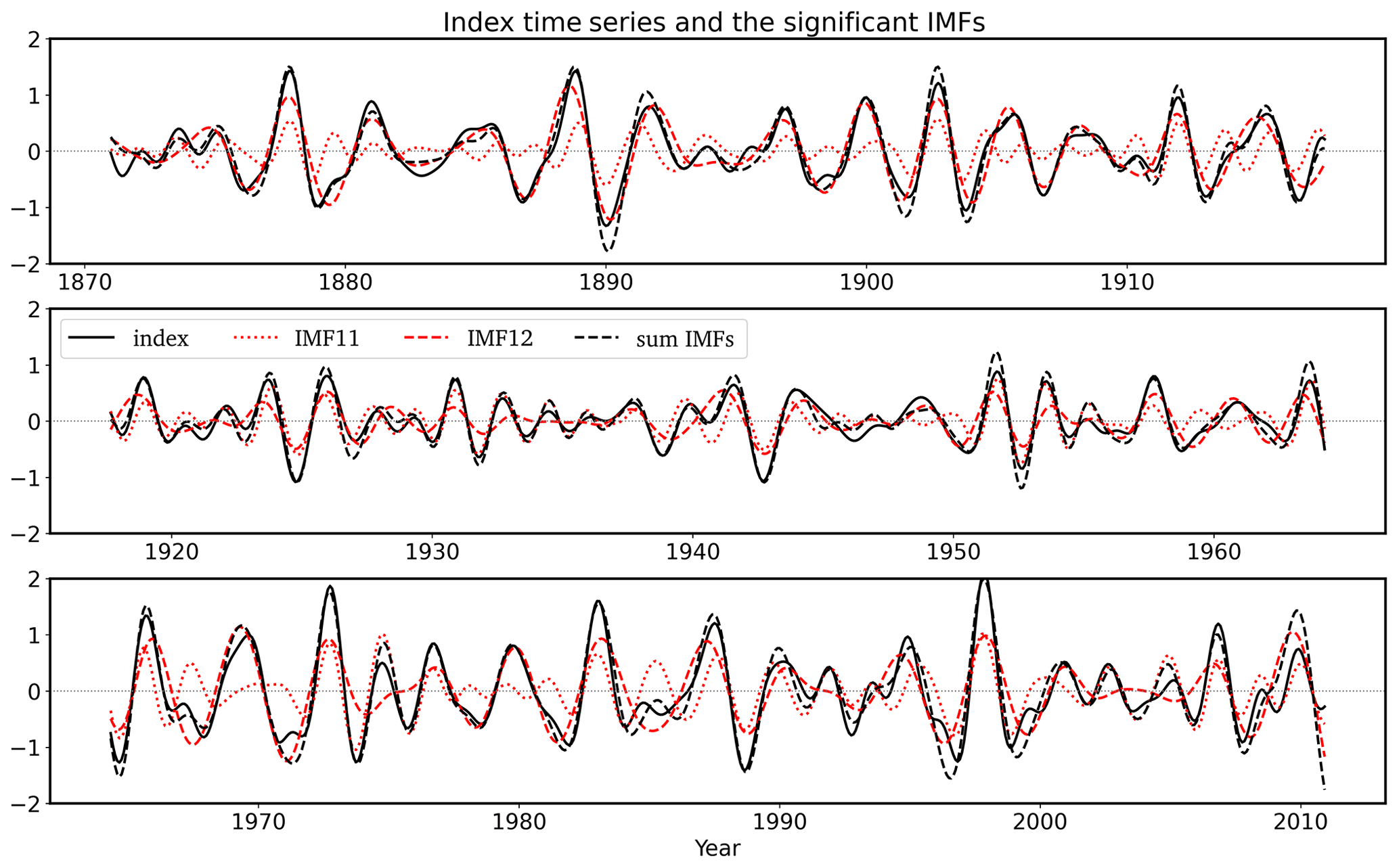
Figure 3Time series (1871–2010) of the Niño3 index from IMF 11 (red dotted line) and IMF 12 (red dashed line) obtained via MEMD. The sum of the two IMF indices (black dashed line) and the band-pass-filtered (16–53 months) Niño3 index (black solid line) are also shown. All data are standardised.
The period/frequency of the two modes is not constant (i.e. varies in time). Thus, we also specify a range of periods/frequencies for the two modes. The mean periods of IMF 11 and 12 with their uncertainty ranges (in square brackets) are: 23 [16, 33] (IMF 11), and 39 [29, 53] (IMF 12) months. These ranges are defined based on the 6.7th and 93.3rd percentiles of IMF 11 and IMF 12's instantaneous period/frequency values, which roughly correspond to ±1.5σ(instantaneous periods). Figure S1 shows power spectra of IMF 11 and IMF 12, which visualise the range of periods the two modes have. Recall that the instantaneous period/frequency can be obtained via Hilbert transform (see Eq. B4 in Appendix B1). This range was chosen as it captures most of the variability in a given mode. Additionally, this range yields a good agreement with other methods (e.g. band-pass filtering), although other (reasonable) percentile ranges give qualitatively similar results. We then use these period/frequency ranges to perform a band-pass filter (via fifth-order Butterworth filter) of the Niño3 index that is consistent with the individual modes (e.g. 29–53-month band of IMF 12 is used to construct band-pass-filtered Niño3 index composites in Fig. 6b; more below). We also use a band-pass filter of the Niño3 index consistent with the sum of the two modes where the band-pass range encompasses periods of both significant modes, i.e. 16–53 months (e.g. used to construct black solid line in Fig. 3).
Time series of the sum of IMFs (black dashed line) and the band-pass index (black solid line) largely agree (i.e. their correlation is 0.95; Fig. 3). Also, the individual modes show very good agreement with the band-passed index, with correlations of 0.68 (IMF 11) and 0.83 (IMF 12), which can be increased further if we consider only the specific IMF's timescale range (specified above) when band-pass filtering the Niño3 index. This merely confirms that MEMD results are consistent with other filtering methods.
Additionally, time series of the Niño3 index extracted from IMF 11 and 12 (Fig. 3) are largely consistent with the modes identified in Jiang et al. (1995) (their Fig. 9a), who used MSSA analysis, and with Wang and Ren (2020) (their Fig. 3), who used EEMD on the Niño3.4 index. IMF 12 is also similar to the Froyland et al. (2021) 4-year mode (their Fig. 10), which used an operator-theoretic approach. The average periods of the significant modes of variability (IMF 11 and 12) in this study are typically lower than in other studies; however, please recall that we have used much longer time series and that the time series of IMFs are nonstationary. Thus, within the overlapping time periods (e.g. recent decades), the timescale (and corresponding time series) is generally consistent across different studies. These similarities provide further confidence in the results from the MEMD. Note that these studies have focused on different ENSO timescales and associated different spatial patterns during QB and LF/QQ ENSO events. However, IMFs are nonstationary and can thus capture changing patterns over time (Sect. 5.3). Also, previous studies have not necessarily considered relationships between different variables that are relevant for the ENSO dynamics (Sect. 6) and related conceptual oscillator models on specific timescales.
Overall, MEMD is consistent with other filtering methods (i.e. it acts like an effective band-pass filter) and can thus be used for further analysis of ENSO dynamics and its nonstationarity to determine if IMFs hold any physical significance. If IMFs have physical meaning, the information inferred from them can be valuable for enhancing climate models, for long-term predictions, for understanding teleconnections, and for exploring the underlying physics and variability of specific fields of interest, such as ENSO. In the following sections we address some of these aspects.
5.3 Nonstationarity of ENSO
The period ranges provided above (see also Fig. S1) suggest that there is some overlap between the period/frequency bands of IMF 11 and IMF 12, which is a result of nonlinear and nonstationary evolution of the modes (period is not constant as seen in Fig. 3). Indeed, there is a low (yet statistically significant) correlation between the two modes (∼ 0.28). Thus, in some time windows the two IMFs can describe the variability of a similar timescale (e.g. similar temporal evolution in Fig. 3 around years 1923–1927, 1951–1955, and 1997), but in other time windows they describe variability on different timescales. Despite changing periods, the two IMFs pass the red noise threshold in the Niño3 region and are therefore still considered significant and thus quasi-periodic (Sects. 4 and 5.1).
In some decades the band-pass-filtered Niño3 index (black solid line) is more consistent with the lower-frequency IMF 12 (red dashed line; approximately 1870–1917 and 1968–2000), and in other periods it is more consistent with the higher-frequency IMF 11 (red dotted line; approximately 1917–1968 and 2000–2010) (Fig. 3). This is consistent with the interdecadal shifts in the frequency of ENSO (Hu et al., 2017, 2020) that have occurred around years 1970 (from higher frequency to lower frequency) and 2000 (from lower frequency to higher frequency). Similar behaviour can also be seen earlier in the record. We can also see interdecadal changes in the amplitude of the ENSO modes, i.e. middle panel (period 1920–1965) in Fig. 3 compared with top and bottom panels (periods 1870–1920 and 1965–2010). This is somewhat consistent with Crespo et al. (2022), who found reduced amplitude of ENSO during the 1901–1931 and 1935–1965 periods relative to the post-1970 period.
Similarly, IMFs can capture different propagation directions of SST anomalies (Fig. 4). Previous studies have highlighted that SST anomaly propagation changed from westward to stationary or eastward around 1970 (Fedorov and Philander, 2000, 2001; Wang and An, 2001). Indeed, the two IMFs show westward propagation of SST anomalies prior to 1970. However, after 1970 it is slightly more complex. SST anomaly propagation becomes stationary or eastward in IMF 11 (except for a period just before 1990; Fig. 4a), but IMF 12 (Fig. 4b) still indicates either stationary or westward propagation with some rare (eastward) exceptions. This is then reflected in the sum of the two modes (Fig. 4c), which generally shows variability in propagation of SST anomalies post-1970. Furthermore, some of the characteristics of SST anomaly propagation from the sum of IMF 11 and IMF 12 carry over to 1-year low-passed SST anomalies (e.g. in the 1960s and 1980s; Fig. 4d).
ENSO events have also been characterised as east Pacific (EP) or central Pacific (CP) depending on the longitude where SST anomalies maximise (e.g. Kao and Yu, 2009; Singh and Delcroix, 2013; Zhang et al., 2019). The two IMFs are less able to reproduce this feature of ENSO diversity (Fig. 4). Most EP events are captured by IMF 11 and 12. However, some CP events (e.g. early 1990s; Fig. 4d) are not captured by quasi-periodic modes of variability (Fig. 4a, b, c). This suggests that other processes are likely causing them, such as sub-ENSO variability (Keenlyside et al., 2007). Similarly, some persistent La Niña events (e.g. mid 1970s, mid-1980s, and around year 2000; Fig. 4d) are not necessarily captured by the quasi-periodic modes of variability alone (potentially related to ENSO asymmetry; e.g. Choi et al., 2013; An et al., 2020). These results could also reflect that some aspects of ENSO nonlinearity are not represented by these two IMFs (e.g. Dommenget et al., 2013).
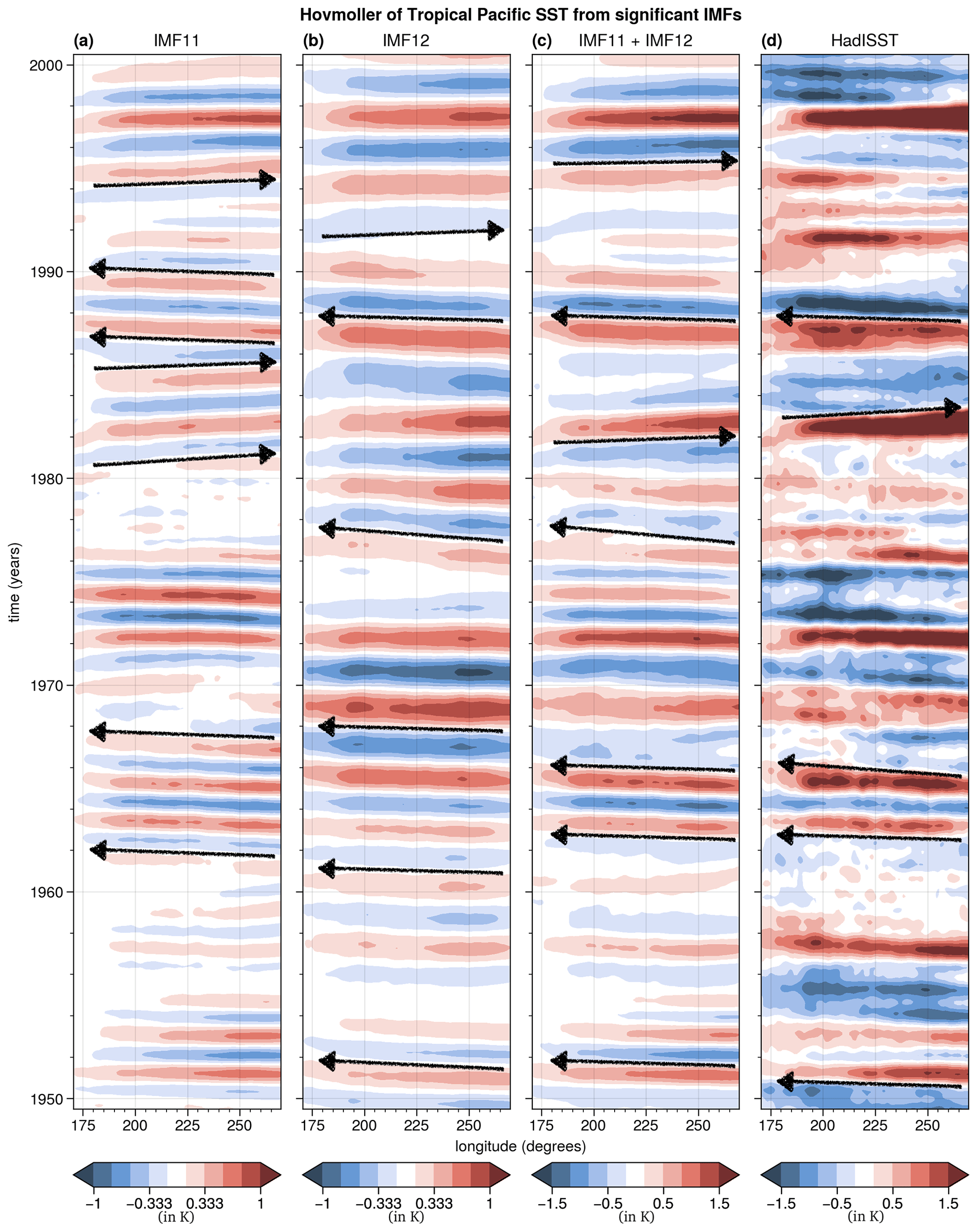
Figure 4Time–longitude Hovmöller diagram of tropical Pacific SST anomalies (in K) averaged between 5∘ S and 5∘ N from (a) IMF 11, (b) IMF 12, (c) IMF 11 + IMF 12, and (d) 1-year low-passed (via fifth-order Butterworth filter) SST data. Black arrows help visualise the direction of propagation of SST anomalies in some periods (other periods are more stationary). We show the time period around year 1970 (1950–2000) where a change in propagation direction has been identified in previous work. Note that the colour scale in panels (a)–(b) is smaller than in panels (c)–(d).
Note that the magnitude of ENSO ultimately depends on all underlying modes of variability in the tropical Pacific (not just on the IMFs discussed here) – as also seen in Fig. 4. In fact, we find ∼ 5 modes (i.e. IMFs 10–14 here) with timescales ranging from ∼ 1 to ∼ 11 years (assessed via the 6.7th and 93.3rd percentiles as above) that can reproduce the majority of the ENSO variability (not shown), but the rest of these modes (i.e. IMF 10, 13, 14 here) are consistent with red noise (Fig. 2).
Figures 3 and 4 also show that weak Niño3 events have either small amplitudes (e.g. 1930–1940) of both IMFs or opposite amplitudes (e.g. 1985–1987). However, strong Niño3 events generally show a constructive interference or mode combination (e.g. 1997, a super-El Niño event), which is consistent with Slawinska and Giannakis (2017), Jajcay et al. (2018), Wang and Ren (2020), and Froyland et al. (2021).
This section has clearly demonstrated that MEMD together with a red noise test is suitable for identifying nonstationary quasi-periodic multivariate signals. This is a clear advantage of MEMD over other multivariate signal processing methods (e.g. PCA, MSSA). Below we now turn to ENSO dynamics to show that IMFs are also physical.
The dynamics of ENSO typically involves positive (e.g. Bjerknes) and negative feedbacks between the atmosphere and ocean. The Bjerknes feedback (Bjerknes, 1969) refers to any decrease (increase) of trade winds that leads to reduced (enhanced) ocean upwelling (downwelling) and thus warming (cooling) in the eastern tropical Pacific, leading to reduced (enhanced) zonal SST and pressure gradients, which in turn reinforce the initial increase (decrease) of the trade winds. The most prominent and also the simplest negative feedback in the tropical Pacific involves recharge/discharge of ocean heat content via Sverdrup transport (e.g. Jin, 1997a, b; Burgers et al., 2005). Other negative feedbacks involve propagation and reflection of ocean Rossby and Kelvin waves (e.g. Suarez and Schopf, 1988; Battisti and Hirst, 1989; Picaut et al., 1997; Weisberg and Wang, 1997; Wang et al., 1999; Wang, 2001, 2018), where the latter can also be wind-forced. These processes generally involve changes in the thermocline depth, surface wind stress, and SST anomalies.
6.1 Quasi-oscillatory timescale
As ENSO dynamics is primarily related to the evolution of the ocean surface zonal wind stress (τx), thermocline depth, and the SST in the tropical Pacific (e.g. Wang, 2018), we demonstrate their relationship with phase composite maps of IMF 12 (Fig. 5). Shading in Fig. 5 represents SST anomalies, contours represent the thermocline depth anomalies (solid contours represent positive values and deeper thermocline), yellow arrows represent τx anomalies, and grey shading represents grid points of the SST that do not pass the red noise threshold. All values are standardised (i.e. divided by standard deviation).
The phase composites are computed using the instantaneous phase of the IMF 12's eastern Pacific SST (Niño3) time series (i.e. IMF 12 (SST (Niño3))) that we can obtain via Hilbert transform (Appendix B1, Eq. B4). This assigns every point in the eastern Pacific SST (Niño3) time series a phase between 0 and 360∘, which can then be split into 12 phases (marked phase 0 through 11; e.g. phase 0 is 0–30∘ and phase 11 is 330–360∘), and all points in the time series (of 1-D or 3-D fields) belonging to a specific phase are then averaged to form map phase composites shown in Fig. 5 (see also Fig. S3 for IMF 11). Line phase composites in Fig. 6 (see also Fig. S4 for IMF 11) are constructed similarly. The eastern Pacific SST (Niño3) is chosen as an index here to focus on east Pacific (EP) ENSO events and related dynamics.
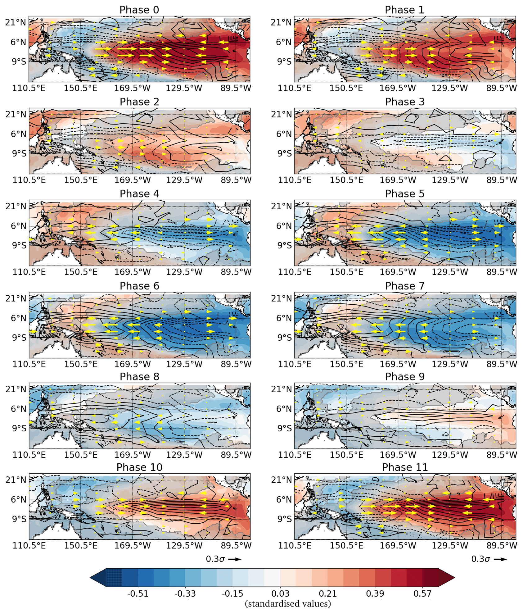
Figure 5Latitude–longitude phase composite (phases 0 to 11 as labelled) of IMF 12: shading for SST, contours for thermocline depth (contour interval is the same as in the colour bar with solid contours representing positive values, and dashed contours represent negative values), and arrows for τx (the scale is shown in the bottom left corner of panels for phases 10 and 11). All data are standardised and all fields were composited based on the phase of the eastern Pacific SST (Niño3) index.
Figure 5 shows a typical cycle of EP ENSO in the tropical Pacific (on a ∼ 3-year timescale) as composited over the IMF 12's Niño3 index. This cycle can also be summarised with line phase composites (Fig. 6a, c) by averaging over specific regions of the tropical Pacific (as labelled; see also Table 1). Here, we analyse the eastern Pacific SST (Niño3), central Pacific τx (Niño4), western Pacific τx (Niño5), off-equatorial western Pacific thermocline depth (Niño6), and Pacific mean thermocline depth as they have historically been considered important for ENSO dynamics and have been used in ENSO conceptual oscillator models (e.g. Jin, 1997a; Burgers et al., 2005; Wang, 2018).
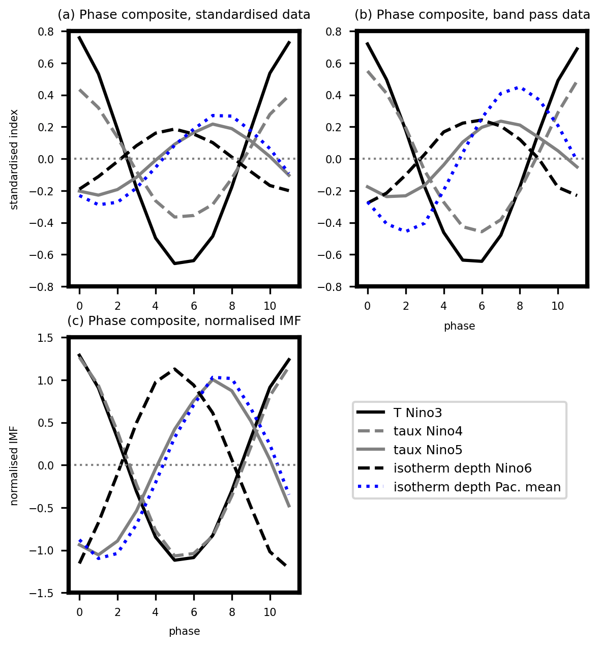
Figure 6Phase composites of the eastern Pacific SST (Niño3) (black solid line), off-equatorial western Pacific isotherm/thermocline depth (Niño6) (black dashed line), Pacific mean isotherm/thermocline depth (blue dotted line), central Pacific τx (Niño4) (grey dashed line), and western Pacific τx (Niño5) (grey solid line). All fields are composited over the phases of the eastern Pacific SST (Niño3), such that they fit the phases in Fig. 5. (a) Composites of IMF 12 for data divided by the standard deviation of the corresponding time series (e.g. IMF 12 (thermocline)/σ (thermocline)); (b) composites of band-pass-filtered (29–53 months) standardised time series; (c) as in panel (a) but IMF time series are divided by IMF's standard deviation (i.e. IMF 12 (thermocline)/σ (IMF 12 of thermocline)).
Together the two figures (Figs. 5, 6a, c) suggest the following sequence of events:
-
during La Niña (phases 5–7) we have negative SST anomalies and a shallower thermocline in the Niño3 region, stronger easterly wind stress in the Niño4 region, and deeper thermocline in the western Pacific (including the Niño6 region);
-
as La Niña weakens (phases 8–10), the westerly wind stress in the Niño5 region and thermocline depth averaged across the tropical Pacific peak, starting the El Niño cycle;
-
as the SST warms, the eastern Pacific thermocline (Niño3) becomes deeper, the central Pacific wind stress (Niño4) becomes westerly, and the thermocline in the western Pacific (including the Niño6 region) becomes shallower (phases 11,0,1);
-
El Niño weakens (phases 2–4), the western Pacific τx (Niño5) becomes easterly, and the thermocline averaged across the Pacific becomes shallower, starting a La Niña event (phases 5–7);
-
the cycle repeats.
The evolution described above is also seen in the band-pass-filtered (29–53 months; 2.5–4.5 years) data (Fig. 6b). Note that the values in Fig. 6b are slightly larger than in Fig. 6a, because slightly different frequency ranges are ultimately represented in the two panels, but they remain qualitatively similar.
While Fig. 6 describes an average evolution of the variables considered, not all individual events have this exact behaviour. This is partly reflected in the reduced amplitudes of τx and thermocline depth in Fig. 6a compared with the SST amplitude. The full time series of these parameters from IMF 12 (Fig. 7; line types/colours are the same as in Fig. 6) show that the relationships from Fig. 6 occur often in the analysed period, especially for strong events. However, for weak events (middle panel in Fig. 7) the relationships are harder to establish – every event seems to be slightly different. This is somewhat consistent with Crespo et al. (2022), who noted that the dynamics of ENSO was different prior to 1970 relative to after 1970, with a dominant recharge–discharge oscillator (Jin, 1997a, b; Burgers et al., 2005) in the latter period.
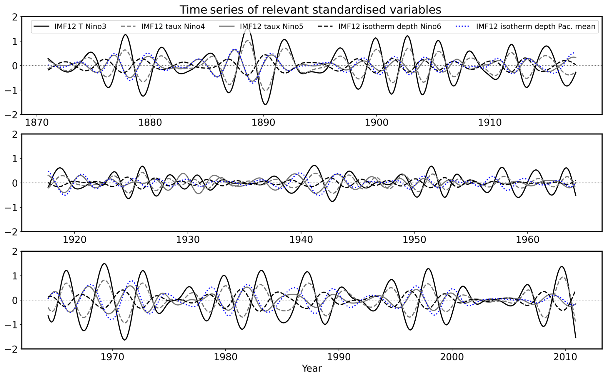
Figure 7IMF 12's standardised time series of the eastern Pacific SST (Niño3) (black solid line), off-equatorial western Pacific thermocline depth (Niño6) (black dashed line), Pacific mean thermocline depth (blue dotted line), central Pacific τx (Niño4) (grey dashed line), and western Pacific τx (Niño5) (grey solid line).
Similar results (phase composites) can also be obtained for the 16–33-month band-passed data and IMF 11 (Figs. S3, S4). This suggests that on average the QB and LF/QQ ENSO events have similar evolution and associated dynamics. However, the frequency of events (see full time series in Fig. S5) that follow the dynamics identified in the phase composites (Fig. S4) is lower in the IMF 11 case than in the IMF 12 case. This may be indicative of other processes that could be relevant for the QB ENSO.
The results presented here and summarised in the line phase composites (Figs. 6, S4) have some interesting implications for the dynamics of ENSO and conceptual oscillator models. The out-of-phase relationship between the Pacific mean thermocline depth (blue dotted line) and eastern Pacific SST (Niño3; black solid line) is a typical feature of the recharge–discharge oscillator (Jin, 1997a, b; Burgers et al., 2005). This suggests that IMFs that emerge from MEMD analysis can capture physical processes in the tropical Pacific. Furthermore, co-variability of the Pacific mean thermocline depth and the western Pacific wind stress (Niño5; grey solid line) suggests that wind forcing in the western Pacific may play a role in the recharge–discharge process or in the onset of ENSO in general as it precedes ENSO events (see also Roulston and Neelin, 2000; Capotondi et al., 2018; Lopez et al., 2013; Lopez and Kirtman, 2014; Timmermann et al., 2018).
On the other hand, the co-variability between the central Pacific wind stress (Niño4; grey dashed line), off-equatorial western Pacific thermocline depth (Niño6; black dashed line), and eastern Pacific SST (Niño3; black solid line) suggests that the unified oscillator proposed by Wang (2001) may need to be revised (see also Graham et al., 2015). This is because (i) in the unified oscillator model these three quantities should all be somewhat out of phase, but here we show that only the western Pacific wind stress and Pacific mean thermocline depth exhibit an out-of-phase relationship with the eastern Pacific SST (on average) and (ii) the Pacific mean thermocline depth does not co-vary with the off-equatorial western Pacific thermocline depth (Niño6), rendering the unified model's recharge–discharge oscillator simplification, which uses the off-equatorial western Pacific thermocline depth (Niño6), questionable.
That the central Pacific wind stress may be omitted in the unified model (due to co-variability with the eastern Pacific SST) was also mentioned in Graham et al. (2015). However, they suggested that western Pacific wind stress (Niño5) could also be omitted from the unified model, but Fig. 6 suggests that on 1.5–4.5-year timescale this variable should be kept. This may be because Graham et al. (2015) used 1-year low-pass-filtered data, which could have obscured the signal on a 1.5–4.5-year timescale (see Sect. 6.2). Additionally, Graham et al. (2015) suggested using the thermocline depth in the western Pacific averaged over a region that lies on the Equator rather than off-Equator. From Fig. 5 we can see that this would likely yield similar results to the off-equatorial western Pacific thermocline depth (Niño6) (to ±1 phase).
6.2 Other timescales
ENSO is a phenomenon that occurs on timescales of 2–8 years, and previous work has often used a 1-year low-pass filter to obtain ENSO. Thus, we now test the relationships between the eastern Pacific SST (Niño3), central Pacific τx (Niño4), western Pacific τx (Niño5), western Pacific off-equatorial thermocline depth (Niño6), and Pacific mean thermocline depth on slightly shorter and slightly longer timescales. We do this to test how relationships between different variables change across timescales that are still somewhat within the ENSO range.
Figure 8 shows phase composites similar to those in Fig. 6b but for band-passed data over a 12–19-month range (shorter periods; Fig. 8a) and over a 42–135-month range (longer periods; Fig. 8b). These timescale bands are consistent with IMF 10 (shorter periods) and IMFs 13 and 14 (longer periods), which are the modes that together with IMF 11 and 12 explain the majority of the variance in the eastern Pacific SST (Niño3).
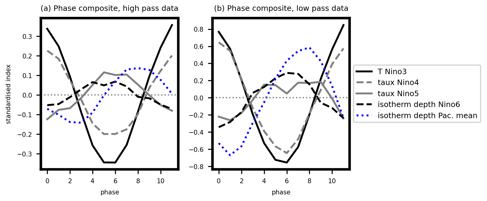
Figure 8As in Fig. 6b but for (a) higher-frequency (band-pass filter over 12–19 months) data and (b) lower-frequency (band-pass filter over 42–135 months) data. Note that higher- and lower-frequency timescale bands were chosen based on timescale ranges of the 10th and 13th–14th IMFs, i.e. the IMFs with slightly smaller or larger (respectively) timescales than IMF 11 and IMF 12.
Interestingly, on these shorter and longer timescales the evolution is different than on quasi-oscillatory timescales (1.5–4.5-year periods of IMF 11 and 12). Namely, the western Pacific wind stress (Niño5) closely follows the western Pacific off-equatorial thermocline depth (Niño6) (Fig. 8a, b). This suggests a very different role of the western Pacific wind stress on different timescales, which may be relevant for ENSO diversity and asymmetry. However, other variables remain similar across timescales (to ±1 phase). Thus, recharge–discharge processes operate throughout the ENSO timescale range (2–8 years), since the Pacific mean thermocline depth and eastern Pacific SST (Niño3) remain out of phase also on these shorter and longer timescales. Also, the results from these shorter and longer timescales indicate that the western Pacific wind stress (Niño5) may be omitted from conceptual oscillator models (on these timescales) as it is anti-correlated with the eastern Pacific SST (Niño3). This is consistent with Graham et al. (2015), who suggested this revision of the unified oscillator, but using 1-year low-pass-filtered data, which may have obscured the different behaviour on quasi-periodic timescales (Sect. 6.1; Fig. 6).
The above analysis shows that it is important to filter the data to correct frequency bands as there may be different behaviour present on different timescales, even within the ENSO range of 2–8 years.
In this study we have used a recently developed nonlinear and nonstationary method for identifying intrinsic variability of multivariate systems, the multivariate empirical mode decomposition (MEMD; Rehman and Mandic, 2010). The method can objectively identify modes of variability on different timescales within a nonlinear and nonstationary dataset describing a complex system such as the climate system. The timescale identification is objective as it is done without any pre-selection of a timescale window in which we expect the quasi-periodic behaviour. It finds a signal that is synchronised across input time series (here PC time series of combined fields, i.e. SST, wind stress, thermocline depth over the tropical Pacific) for every timescale within the given system. Also, the multivariate modes of variability that emerge from the MEMD analysis have nonstationary (i.e. evolving in time) patterns of variability (e.g. Fig. 4) – a clear advantage over some other multivariate time series analysis tools whose patterns are stationary.
Additionally, a red noise significance test has been developed to robustly identify quasi-periodic modes of variability in the given data, which had not been used before in the framework of MEMD. This means that MEMD can now be used as an alternative method for objective identification of the timescale of quasi-periodic motions in the climate system. Since the red noise test can be applied on every grid point separately, MEMD together with the red noise test can also be used for identifying potential new regions of quasi-periodic variability (similar to Fig. 5).
We demonstrate that MEMD can identify physical quasi-periodic modes of variability within the climate system by analysing the tropical Pacific SST variability. We have identified a clear quasi-periodic behaviour on a timescale of about 2–3 years (16–53 months) in the tropical Pacific. This timescale falls within the typical timescale range of ENSO, i.e. 2–8 years, and the dynamics of this quasi-periodic variability is consistent with ENSO dynamics. While ENSO quasi-periodic variability is well known, an identification (via MEMD) of a frequency range linked to the two dominant quasi-periodic modes of variability (i.e. 16–53 months) has still led to a few interesting results.
By analysing composites (e.g. Figs. 5, 6) of the thermocline depth, wind stress, and SST, we have shown that the ∼ 2–3-year (eastern Pacific) ENSO variability is generally consistent with the recharge–discharge conceptual oscillator model of ENSO (e.g. Jin, 1997a; Burgers et al., 2005). This oscillator describes an interplay between the Pacific mean thermocline depth and eastern Pacific SST (Niño3), which are related to recharge and discharge of ocean heat content on a timescale of about 3 years. However, the unified model (Wang, 2001) may need to be revised (see also Graham et al., 2015) as most of the variables relevant for the unified oscillator model co-vary. In particular, the western Pacific off-equatorial thermocline depth (Niño6), central Pacific wind stress (Niño4), and eastern Pacific SST (Niño3) exhibit the same phase relation and thus describe the same dynamics. As also the western Pacific wind stress (Niño5; relevant for the unified oscillator) and Pacific mean thermocline depth co-vary, there seems to be a close relationship between the recharge–discharge and unified oscillator models, but it may be different than previously thought.
On shorter and longer timescales (12–19 months and 42–135 months; Fig. 8) the relationships between variables are different; in particular, the western Pacific wind stress (Niño5) on these timescales co-varies with the eastern Pacific SST (Niño3). This suggests that the role of the western Pacific atmosphere–ocean processes (via wind stress) in tropical Pacific variability (and ENSO) can be very different on different timescales, whereas other variables (and in other regions) largely keep their relationships across timescales. This means that the recharge–discharge oscillator model operates on all timescales considered (12–135 months), even if it has a characteristic timescale. However, the relations underlying the unified oscillator model exhibit different behaviour on different timescales, the implications of which should be explored further in the future.
MEMD analysis could be extended in several ways, for example (i) to assess ENSO dynamics in models as they typically struggle with the representation of the western Pacific processes (i.e. relevant for Niño5 wind stress; Guilyardi et al., 2020; Planton et al., 2021) and (ii) to study ENSO teleconnections on different timescales (e.g. Brönnimann, 2007; Fereday et al., 2008; Jiménez-Esteve and Domeisen, 2018, 2020; Hardiman et al., 2019). Also, future studies should involve an examination of sensitivity and causal links (not established here) between different variables and their links across scales (e.g. Runge et al., 2015; Jajcay et al., 2018; Jenney et al., 2019; Kretschmer et al., 2021), as well as dedicated model experiments.
Overall, this study has analysed the variability in the tropical Pacific (using MEMD with a red noise test), identified two quasi-periodic modes of variability (on ∼ 2–3-year timescale), related their physics to the recharge–discharge oscillator, and suggested a revision to the unified oscillator model (somewhat consistent with Graham et al., 2015). As the variability on this timescale is quasi-periodic, it may be predictable far in advance, which calls for further investigations of the tropical Pacific variability and related teleconnections, for their prediction, and for further model improvements (see also Chen et al., 2021; Lee et al., 2021).
To find the intrinsic variability of our 3-D field, i.e. mentioned in Sect. 3.3, we first reduce the dimensionality of our data by decomposing it using the singular value decomposition (SVD), which yields spatial patterns of our data (empirical orthogonal functions, EOFs) and corresponding time series (principal components, PCs). First, we multiply A′ by (area weighting; with ϕ latitude), divide by standard deviation (σ) at each grid point (and for each variable separately, if relevant), and reshape A′ from a 3-D array to a 2-D array . Then A′ can be expressed with a singular value decomposition as
where U and V represent the left and right singular vectors related to PCs and EOFs, is a diagonal matrix with square roots of the explained variance of each mode (denoted Λ, i.e. eigenvalues) along the diagonal, Lt is the length of time series, and superscript T denotes transpose. PCs are defined as and EOFs as , such that can be represented as a function of PCs and EOFs:
where m corresponds to the PC number and is ordered according to the eigenvalues (m=1 for the largest eigenvalue). We retain only the leading 20 PCs for the analysis (they generally describe the majority of the variance in A′).
Now we can use the 20 PCs (PC(m,Lt)) as input to the MEMD algorithm (for details on the algorithm itself see Rehman and Mandic, 2010). This algorithm finds common timescales (i.e. intrinsic mode functions, IMFs) within the 20 PCs and splits each PC into several IMFs (the number of IMFs is not predetermined). Thus, each PC can be represented as a sum of IMFs
where s corresponds to IMF number and is ordered according to the timescale (s=1 for the shortest timescale and smax for the longest timescale, which is usually a trend or a residual). Equation (A3) shows that each PC is a superposition of different IMFs (see also Table S2) and with it also a superposition of modes of variability in the selected field(s) with different timescales.
Each PC is associated with a spatial pattern (EOF), which allows a reconstruction of the time–space structure/evolution for each IMF, yielding IMFs of the initial dataset A′ (IMFA). We do this by multiplying PCs for each IMF with corresponding EOFs and summing over all 20 PCs/EOFs (similar to Eq. A2):
Here note that to get IMFA in the units of the input field we must multiply it by the field's standard deviation as the input data for the SVD algorithm were standardised (Eq. A1). Again, IMFAs are ordered by timescale, i.e. IMFA1 with the shortest timescale and IMFAsmax with the longest timescale (trend). From here we can reconstruct A′ by summing over all IMFAs,
and ultimately one can also reshape A′ from a 2-D array to a 3-D array . The importance of each IMFA for A′ can be assessed by computing the explained variance of each IMFA or other significance methods. To find IMFA modes (and grid points) that correspond to potentially oscillatory behaviour we must perform a red noise test (see Appendix B).
Note that from here on (and in the main text) IMFAs are referred to as IMFs for simplicity.
Typically we can test if the modes (IMFs) are different from white or red noise, depending on the distribution of our data. In the climate system, variables often exhibit behaviour that resembles white or red noise. The IMFs that are significant (i.e. different from both red and white noise) likely represent quasi-oscillations, indicating higher potential for predictability of processes that correspond to the timescale of the significant IMF. Thus, this distinction is very important in climate science. Therefore, we discuss the white and red noise tests (for 1-D data, i.e. time series) below, whereas the robustness of IMFs from the MEMD analysis and the relevant significance tests are discussed in the main text (Sects. 4 and 5).
Note that the white and red noise tests are performed on 1-D time series; hence, EMD (univariate decomposition; see main text) is first used to test the performance of IMFs that arise from the EMD analysis. The multivariate data (via MEMD) in the main text are analysed with the simplest and most relevant test (i.e. theoretical red noise test described below).
B1 White noise test
The white noise significance test has been derived by Wu and Huang (2004), who showed that the energy density function of the sth IMF (Es; i.e. average squared amplitude of the sth IMF) is
where IMFs(j) is the sth IMF at time step j (), and Lt is the length of the time series. Wu and Huang (2004) further showed that the total energy density of the sth IMF can then be expressed as
where ν is frequency, and S(ν)s is the power spectrum of the sth IMF. From this they showed that for white noise,
where Ts is the average period of the sth IMF, and ln denotes the natural logarithm.
Note that the frequency (and thus also period) of each IMF is computed using Hilbert transform by first generating an analytical signal (e.g. Huang et al., 1998):
where t is time dimension, X(t) is our IMF time series, Y(t) is its Hilbert transform, Z(t) is the analytical signal, and is the instantaneous phase. The instantaneous frequency can then be computed by taking a time derivative of the phase, i.e. , and the average frequency of each IMF is computed by averaging the instantaneous frequency in time (note that period = , i.e. Ts).
The relationship between the logarithms of energy density and average period of the IMFs (Eq. B3) is then used in Fig. B1a (black solid line) to test whether an IMF (using EMD of the Niño3 index; blue dots in Fig. B1a; see also Sect. 3) is different from white noise or not. The mode is significant with respect to white noise if it exceeds the one-tailed 95th percentile threshold (denoted by the black dotted line). The percentile range serves as a significance test; i.e. if IMFs from our data are above, for example, the 95th percentile they are significant at the 95th percentile level. The percentile range can be expressed analytically as (Wu and Huang, 2004)
where p denotes a threshold (p=1.645 for the one-tailed 95th percentile of the Gaussian distribution). Note that typically the number of degrees of freedom (DoFs) for white noise data is expected to be equal to the total energy density of the sth IMF (i.e. DoFs=LtEs; Wu and Huang, 2004).
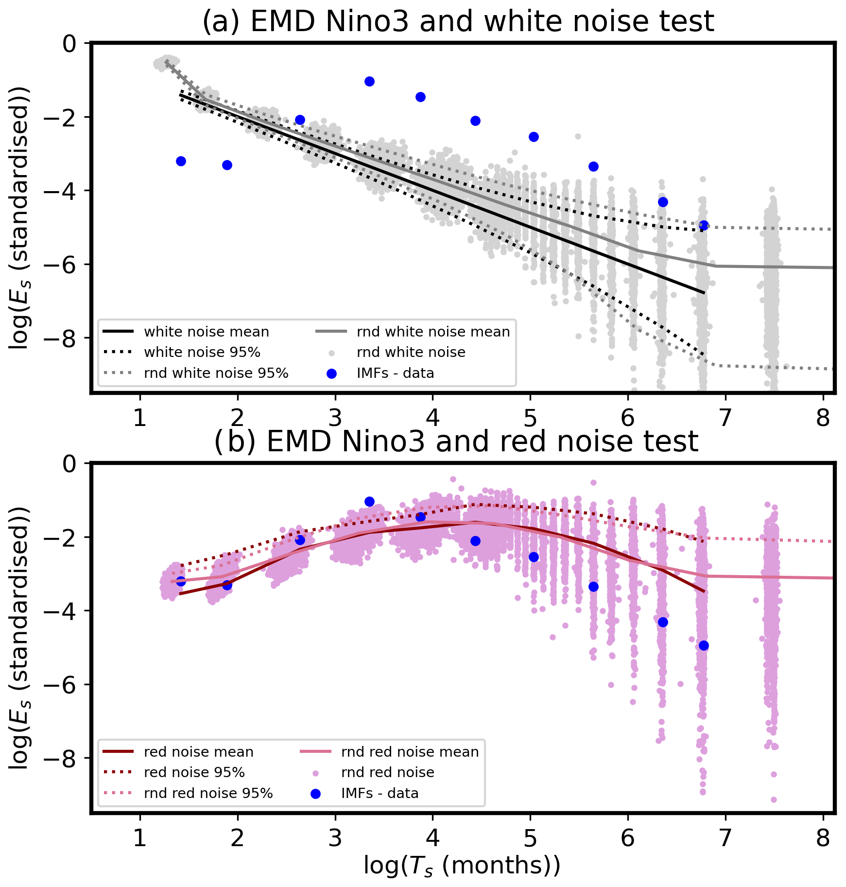
Figure B1Significance tests for EMD modes: (a) the white noise significance test and (b) the red noise significance test for EMD IMFs of the Niño3 index (blue dots). Blue dots are computed as in Fig. 2. (a) The black solid line represents the theoretical linear relationship between the logarithm of the average period (Ts) and the logarithm of energy density (Es; i.e. average squared amplitude; Eq. B3); the black dotted line represents 5th–95th percentile (Eq. B5); the grey dots represent I=Lt realisations of IMFs of white noise time series (the length is the same as for the Niño3 index), whereas the grey solid and dotted lines represent their mean and the 5th–95th percentile, respectively. (b) The red solid line represents the theoretical red spectrum energy density (Eqs. B7–B9); the red dotted line represents the 95th percentile (via χ2 test); the light pink dots represent I=Lt realisations of IMFs of the red noise time series (Eq. B6; the length Lt is the same as for the Niño3 index), whereas the pink solid and dotted lines represent their mean and the 95th percentile, respectively. Note that the x axis shows the logarithms of the period (log e(Ts)) ordered from the shortest period (highest frequency) to the longest period (trend). For further descriptions of the figure see text.
Alternatively, we can test whether the input data are different from white noise by constructing multiple (I) realisations of synthetic white noise time series wi (ith random normally distributed time series with standard deviation σ of 1). Then we can compute its IMFs via EMD (Sect. 3), and we can repeat the process I times. Employing Eq. B1 on these IMFs yields scattered grey dots in Fig. B1a (constructed in the same way as blue dots; see also Sect. 4, Fig. 2), where their mean and 5th–95th percentile are shown as grey solid and dotted lines, respectively.
A comparison with the IMFs from the input data (Niño3 index; blue dots in Fig. B1a) reveals that many IMFs lie outside the white noise range and that overall the data (blue dots) distribution does not resemble the white noise (grey dots) distribution (not noted in Wu and Huang, 2004). This suggests that a white noise test for such data is not a good test. Indeed, atmosphere–ocean coupled systems, such as ENSO, can often be represented as a red noise process (e.g. Hasselmann, 1976; Frankignoul and Hasselmann, 1977); thus, we now turn to a similar test but for data distributed as red noise.
B2 Red noise test
B2.1 Synthetic red noise data
To test if our data (e.g. Niño3 index) is purely red noise or it has inherent oscillations that we can identify through the (M)EMD analysis, we generate I realisations of synthetic red noise time series x (AR(1) process) as (e.g. Gilman et al., 1963)
where r is the lag-1 auto-correlation from our data (e.g. Niño3 index), w is white noise (as in Appendix B1), i runs over I realisations of synthetic red noise data, and j (j>1 and j≤Lt; with Lt length of our data, e.g. the length of Niño3 record) is an index that runs over the time steps (one time step is one time unit, e.g. 1 month). For j=1 (the first time step) we set .
Once we obtain the red noise time series xi we can compute its IMFs via EMD (Sect. 3) and we can repeat the process I times (as for the white noise; Appendix B1). This yields the pink scattered dots in Fig. B1b. The mean over I cases for each IMF (frequency band) is shown by the pink solid line, and the (one-tailed) 95th percentile across the I cases is shown by the pink dotted line. Note that we plot logarithmic values in Fig. B1, as mentioned above.
Note that Franzke (2009) used a similar approach for indices such as the North Atlantic Oscillation and found a simple relationship between the power spectrum and frequency, consistent with Kolotkov et al. (2016). However, we follow Gilman et al. (1963) to define a relationship between the power spectrum and frequency. This incorporates the lag-1 auto-correlation of the time series into the theoretical red noise power spectrum (see below).
B2.2 Theoretical red noise test
Alternatively, one can compute a theoretical power spectrum of the red noise (see Gilman et al., 1963):
where S is the power spectrum of red noise, is the frequency, and r is again the lag-1 auto-correlation from our data. For each frequency estimate we must multiply S(ν) by the frequency range (Δν) (as in Eq. B2) to obtain a theoretical estimate of the (mean) energy of the red noise (Ered) (cf. Kolotkov et al., 2016):
where and with s running over frequencies (from higher to lower frequency). Note that since EMD is a dyadic filter (each lower frequency is a half of the previous one; e.g. Flandrin et al., 2004; Rehman and Mandic, 2011) both α and β typically take a value of (consistent with Kolotkov et al., 2016). However, when mode mixing is present (e.g. here it is generally present at higher and lower frequencies of IMFs from MEMD analysis) this is not necessarily true, hence the use of α and β in Eq. (B8). Finally, Ered for every sth IMF (i.e. ) must be scaled such that its total energy is the same as the total energy of our data (e.g. Madden and Julian, 1971; Bretherton et al., 1999):
where smax is the number of IMFs (as above), and s represents the sth IMF of frequency νs; Es was defined previously (Eq. B1). Note that we scale from total energies of IMFs between s=2 and as the last IMF is typically a trend/residual and the first IMF does not necessarily follow the distribution correctly (but including the two usually does not significantly alter the results). is shown in Fig. B1b as a red solid line.
This red noise test is typically used in climate science to determine the significance of power spectra peaks in our data (using S(ν) from Eq. B7), and it differs from the red noise test of Kolotkov et al. (2016) as it takes into consideration the lag-1 auto-correlation of the data. If the cosine function in the S(ν) (Eq. B7) is expanded into the Taylor series () one can realise that for large ν (high frequencies) S(ν) indeed reduces to the spectrum γν−2 (with γ a constant) suggested by Kolotkov et al. (2016); Franzke (2009). However, for low frequencies (small ν) they do not agree well and ultimately S(ν) also becomes a constant (see Fig. B2 for comparison). Furthermore, as S(ν) depends on the lag-1 auto-correlation (r), we can see from Eq. (B7) that for r=0, S(ν)=1; i.e. it reduces to the power spectrum of the white noise. This means that this theoretical test can potentially be used for testing the significance of the data that correspond to either white or red noise.
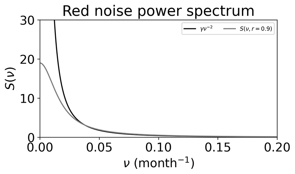
Figure B2Red noise power spectrum (S(ν)) for (black line) and (grey line) S(ν,r) from Eq. (B7) for r=0.9. γ was estimated as a ratio between the integrated power spectra of the two spectra for frequencies higher than 0.02 per month () where the two power spectra generally agree well.
The significance of the IMFs from the input data is tested using a χ2 test, where the sth IMF's value for the (one-tailed) 95th percentile is computed from DoFs=LeffEs degrees of freedom (instead of LtEs as was the case for white noise, due to strong correlations between neighbouring data points; Bretherton et al., 1999; Wu and Huang, 2004; Kolotkov et al., 2016), where
Then we multiply the expected red noise curve by (e.g. Madden and Julian, 1971; Bretherton et al., 1999) to ultimately obtain a threshold for the 95th percentile (red dotted line in Fig. B1b). Note that for DoFs<1 we set DoFs=1 (to avoid numerical issues). The IMFs derived from the data (blue dots in Fig. B1b) that exceed the red noise threshold (i.e. lie above the red/pink dotted line in Fig. B1b) are considered significant at the 95th percentile (one-tailed).
Figure B1b shows that the two (synthetic and theoretical) red noise tests (for the Niño3 index via EMD) are somewhat comparable and that the majority of the input (e.g. Niño3 index) data (blue dots) lie within the red noise range (i.e. within the pink dots and below the pink/red dotted line). However, we can identify one IMF (period ∼ 31 months or ∼ 2.5 years) that is above the red noise threshold and well within the typical ENSO timescale (2–8 years), suggesting quasi-periodic behaviour (oscillations).
Similarly, we can use the theoretical red noise significance test on IMFs obtained via MEMD, which yields two significant modes of variability in the eastern Pacific SST (Niño3) index (see the main text). Note, however, that we do not necessarily expect exactly the same results from the EMD (Fig. B1b) and MEMD (Fig. 2) methods since the MEMD finds a synchronised signal within the tropical Pacific and across different variables, whereas EMD only analyses the 1-D Niño3 time series. This is also true for the number of IMFs obtained via the two different methods. MEMD yields significantly more IMFs as EMD (21 versus 10), which is likely a result of inputting several different time series with different timescales, especially in the high- and low-frequency range (i.e. periods shorter than about 8 months and longer than about 700 months).
Alternatively, one can also compute significant modes by computing the red noise test at each grid point and then average the results over all grid points, but we have not used this here. Instead, we use an additional test on map plots in Sect. 5 (Figs. 5 and S3), where we identify potentially oscillatory grid points and use grey shading on areas that are well represented with red noise alone (i.e. not significant).
Despite some differences between the MEMD and EMD modes of variability (primarily due to different input time series), the two methods agree on the quasi-periodic timescale of 2–3 years in the Niño3 region. This is also consistent with the significant periods inferred from the usual 1-D wavelet transform (not shown) and the power spectrum analysis of the Niño3 index (1-D) obtained via Fourier transform (Fig. B3). The latter confirms that the 2–3-year timescale is quasi-periodic as there is a significant peak in the power spectrum of the Niño3 index on those timescales; i.e. the black solid line in Fig. B3 (Niño3 index) is above the red dashed line (red noise one-tailed 95 % threshold).
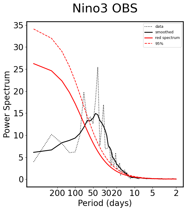
Figure B3Power spectrum of the Niño3 index. The power spectra are first computed for 500-month-long chunks (overlapped by 250 months) and then averaged over all cases (grey solid line). The black solid line represents a 10-point running mean of the black dotted line (to increase the number of degrees of freedom, which is ; see also Boljka et al., 2021). The red solid and dashed lines represent the theoretical red noise test and its (one-tailed) 95th percentile, respectively.
EMD and MEMD Python codes are available on GitHub (https://doi.org/10.5281/zenodo.5459184, Laszuk, 2017), https://github.com/mariogrune/MEMD-Python-, Rehman and Mandic, 2010). Other scripts are available upon request.
SODA2 data can be downloaded from http://apdrc.soest.hawaii.edu/dods/public_data/SODA/soda_pop2.2.4 (Carton and Giese, 2008); HadISST data can be downloaded from https://www.metoffice.gov.uk/hadobs/hadisst (Rayner et al., 2023).
The supplement related to this article is available online at: https://doi.org/10.5194/wcd-4-1087-2023-supplement.
LB performed the analysis, prepared the figures, and wrote the first draft of the manuscript. NEO and NSK provided additional insight and helped improve the manuscript for the final version.
The contact author has declared that none of the authors has any competing interests.
This work reflects the analysis and views of the author Lina Boljka. No reader should interpret this work to present the views of any third party. Assumptions, opinions, views, and estimates constitute the author's judgement as of the date given and are subject to change without notice and without duty to update.
Publisher’s note: Copernicus Publications remains neutral with regard to jurisdictional claims made in the text, published maps, institutional affiliations, or any other geographical representation in this paper. While Copernicus Publications makes every effort to include appropriate place names, the final responsibility lies with the authors.
This work was supported by the Trond Mohn Foundation (project BCPU, grant no. BFS2018TMT01) and was performed on NIRD/Sigma2 (project NS9039K). Noel S. Keenlyside and Nour-Eddine Omrani acknowledge support from the Research Council of Norway (grant no. 312017, RACE; grant no. 316618, ROADMAP). We thank three anonymous reviewers and William Roberts for their constructive comments that helped improve the original manuscript. We also thank Lander Crespo for helpful discussions and Ingo Bethke for help with the data.
This research has been supported by the Trond Mohn stiftelse (grant no. BFS2018TMT01) and the Research Council of Norway (grant no. 312017, RACE; grant no. 316618, ROADMAP).
This paper was edited by William Roberts and reviewed by three anonymous referees.
Alberti, T., Donner, R. V., and Vannitsem, S.: Multiscale fractal dimension analysis of a reduced order model of coupled ocean–atmosphere dynamics, Earth Syst. Dynam., 12, 837–855, https://doi.org/10.5194/esd-12-837-2021, 2021. a, b
Allan, R. J.: ENSO and Climatic Variability in the Past 150 Years, 3–56, Cambridge University Press, https://doi.org/10.1017/CBO9780511573125.002, 2000. a, b
An, S.-I., Tziperman, E., Okumura, Y. M., and Li, T.: ENSO Irregularity and Asymmetry, Chap. 7, American Geophysical Union (AGU), 153–172, https://doi.org/10.1002/9781119548164.ch7, 2020. a
Ashok, K., Behera, S. K., Rao, S. A., Weng, H., and Yamagata, T.: El Niño Modoki and its possible teleconnection, J. Geophys. Res.-Oceans, 112, C11007, https://doi.org/10.1029/2006JC003798, 2007. a
Baede, A., Ahlonsou, E., Ding, Y., and Schimel, D.: The Climate System: an Overview, Cambridge University Press, Cambridge, United Kingdom and New York, NY, USA, 1–881, https://www.ipcc.ch/report/ar3/wg1/chapter-1-the-climate-system-an-overview/ (last access: 4 December 2023), 2001. a
Battisti, D. S. and Hirst, A. C.: Interannual Variability in a Tropical Atmosphere–Ocean Model: Influence of the Basic State, Ocean Geometry and Nonlinearity, J. Atmos. Sci., 46, 1687–1712, https://doi.org/10.1175/1520-0469(1989)046<1687:IVIATA>2.0.CO;2, 1989. a
Bejarano, L. and Jin, F.-F.: Coexistence of Equatorial Coupled Modes of ENSO, J. Climate, 21, 3051–3067, https://doi.org/10.1175/2007JCLI1679.1, 2008. a
Bjerknes, J.: ATMOSPHERIC TELECONNECTIONS FROM THE EQUATORIAL PACIFIC, Mon. Weather Rev., 97, 163–172, https://doi.org/10.1175/1520-0493(1969)097<0163:ATFTEP>2.3.CO;2, 1969. a
Boljka, L., Thompson, D. W. J., and Li, Y.: Downstream Suppression of Baroclinic Waves, J. Climate, 34, 919–930, https://doi.org/10.1175/JCLI-D-20-0483.1, 2021. a
Bretherton, C. S., Widmann, M., Dymnikov, V. P., Wallace, J. M., and Bladé, I.: The Effective Number of Spatial Degrees of Freedom of a Time-Varying Field, J. Climate, 12, 1990–2009, https://doi.org/10.1175/1520-0442(1999)012<1990:TENOSD>2.0.CO;2, 1999. a, b, c, d, e, f
Broomhead, D. S., Jones, R., and King, G. P.: Topological dimension and local coordinates from time series data, J. Phys. A-Math. Gen., 20, L563–L569, https://doi.org/10.1088/0305-4470/20/9/003, 1987. a
Brönnimann, S.: Impact of El Niño–Southern Oscillation on European climate, Rev. Geophys., 45, RG3003, https://doi.org/10.1029/2006RG000199, 2007. a
Burgers, G., Jin, F.-F., and van Oldenborgh, G. J.: The simplest ENSO recharge oscillator, Geophys. Res. Lett., 32, L13706, https://doi.org/10.1029/2005GL022951, 2005. a, b, c, d, e
Capotondi, A., Sardeshmukh, P. D., and Ricciardulli, L.: The Nature of the Stochastic Wind Forcing of ENSO, J. Climate, 31, 8081–8099, https://doi.org/10.1175/JCLI-D-17-0842.1, 2018. a
Carton, J. A. and Giese, B. S.: A Reanalysis of Ocean Climate Using Simple Ocean Data Assimilation (SODA), Mon. Weather Rev., 136, 2999–3017, https://doi.org/10.1175/2007MWR1978.1, 2008 (data available at: http://apdrc.soest.hawaii.edu/dods/public_data/SODA/soda_pop2.2.4). a
Chen, H.-C., Jin, F.-F., Zhao, S., Wittenberg, A. T., and Xie, S.: ENSO Dynamics in the E3SM-1-0, CESM2, and GFDL-CM4 Climate Models, J. Climate, 34, 9365–9384, https://doi.org/10.1175/JCLI-D-21-0355.1, 2021. a
Choi, K.-Y., Vecchi, G. A., and Wittenberg, A. T.: ENSO Transition, Duration, and Amplitude Asymmetries: Role of the Nonlinear Wind Stress Coupling in a Conceptual Model, J. Climate, 26, 9462–9476, https://doi.org/10.1175/JCLI-D-13-00045.1, 2013. a
Crespo, L. R., Rodríguez-Fonseca, M. B., Polo, I., Keenlyside, N., and Dommenget, D.: Multidecadal variability of ENSO in a recharge oscillator framework, Environ. Res. Lett., 17, 074008, https://doi.org/10.1088/1748-9326/ac72a3, 2022. a, b, c, d
de la Cámara, A., Birner, T., and Albers, J. R.: Are Sudden Stratospheric Warmings Preceded by Anomalous Tropospheric Wave Activity?, J. Climate, 32, 7173–7189, https://doi.org/10.1175/JCLI-D-19-0269.1, 2019. a, b
Dommenget, D., Bayr, T., and Frauen, C.: Analysis of the non-linearity in the pattern and time evolution of El Niño southern oscillation, Clim. Dynam., 40, 2825–2847, https://doi.org/10.1007/s00382-012-1475-0, 2013. a, b
Duffy, D. G.: The Application of Hilbert–Huang Transforms to Meteorological Datasets, J. Atmos. Ocean. Tech., 21, 599–611, https://doi.org/10.1175/1520-0426(2004)021<0599:TAOHTT>2.0.CO;2, 2004. a
Ezer, T. and Corlett, W. B.: Is sea level rise accelerating in the Chesapeake Bay? A demonstration of a novel new approach for analyzing sea level data, Geophys. Res. Lett., 39, L19605, https://doi.org/10.1029/2012GL053435, 2012. a
Ezer, T., Atkinson, L. P., Corlett, W. B., and Blanco, J. L.: Gulf Stream's induced sea level rise and variability along the U.S. mid-Atlantic coast, J. Geophys. Res.-Oceans, 118, 685–697, https://doi.org/10.1002/jgrc.20091, 2013. a
Fedorov, A. V. and Philander, S. G.: Is El Niño Changing?, Science, 288, 1997–2002, https://doi.org/10.1126/science.288.5473.1997, 2000. a, b
Fedorov, A. V. and Philander, S. G.: A Stability Analysis of Tropical Ocean–Atmosphere Interactions: Bridging Measurements and Theory for El Niño, J. Climate, 14, 3086–3101, https://doi.org/10.1175/1520-0442(2001)014<3086:ASAOTO>2.0.CO;2, 2001. a
Fereday, D. R., Knight, J. R., Scaife, A. A., Folland, C. K., and Philipp, A.: Cluster Analysis of North Atlantic–European Circulation Types and Links with Tropical Pacific Sea Surface Temperatures, J. Climate, 21, 3687–3703, https://doi.org/10.1175/2007JCLI1875.1, 2008. a
Flandrin, P., Rilling, G., and Goncalves, P.: Empirical mode decomposition as a filter bank, IEEE Signal Proc. Let., 11, 112–114, https://doi.org/10.1109/LSP.2003.821662, 2004. a
Frankignoul, C. and Hasselmann, K.: Stochastic climate models, Part II Application to sea-surface temperature anomalies and thermocline variability, Tellus, 29, 289–305, https://doi.org/10.3402/tellusa.v29i4.11362, 1977. a, b
Franzke, C.: Multi-scale analysis of teleconnection indices: climate noise and nonlinear trend analysis, Nonlinear Proc. Geoph., 16, 65–76, https://doi.org/10.5194/npg-16-65-2009, 2009. a, b, c
Franzke, C.: Nonlinear Trends, Long-Range Dependence, and Climate Noise Properties of Surface Temperature, J. Climate, 25, 4172–4183, https://doi.org/10.1175/JCLI-D-11-00293.1, 2012. a
Franzke, C. and Woollings, T.: On the Persistence and Predictability Properties of North Atlantic Climate Variability, J. Climate, 24, 466–472, https://doi.org/10.1175/2010JCLI3739.1, 2011. a
Froyland, G., Giannakis, D., Lintner, B., Pike, M., and Slawinska, J.: Spectral analysis of climate dynamics with operator-theoretic approaches, Nat. Commun., 12, 6570, https://doi.org/10.1038/s41467-021-26357-x, 2021. a, b, c, d
Ghil, M., Allen, M. R., Dettinger, M. D., Ide, K., Kondrashov, D., Mann, M. E., Robertson, A. W., Saunders, A., Tian, Y., Varadi, F., and Yiou, P.: Advanced spectral methods for climatic time series, Rev. Geophys., 40, 3–1–3–41, https://doi.org/10.1029/2000RG000092, 2002. a
Gilman, D. L., Fuglister, F. J., and Mitchell, J. M.: On the power spectrum of “red noise”, J. Atmos. Sci., 20, 182–184, 1963. a, b, c, d, e
Graham, F. S., Brown, J. N., Wittenberg, A. T., and Holbrook, N. J.: Reassessing Conceptual Models of ENSO, J. Climate, 28, 9121–9142, https://doi.org/10.1175/JCLI-D-14-00812.1, 2015. a, b, c, d, e, f, g
Guilyardi, E., Capotondi, A., Lengaigne, M., Thual, S., and Wittenberg, A. T.: ENSO Modeling, Chap. 9, American Geophysical Union (AGU), 199–226, https://doi.org/10.1002/9781119548164.ch9, 2020. a
Hardiman, S. C., Dunstone, N. J., Scaife, A. A., Smith, D. M., Ineson, S., Lim, J., and Fereday, D.: The Impact of Strong El Niño and La Niña Events on the North Atlantic, Geophys. Res. Lett., 46, 2874–2883, https://doi.org/10.1029/2018GL081776, 2019. a
Hasselmann, K.: Stochastic climate models Part I. Theory, Tellus, 28, 473–485, https://doi.org/10.1111/j.2153-3490.1976.tb00696.x, 1976. a, b
Hasselmann, K.: PIPs and POPs: The reduction of complex dynamical systems using principal interaction and oscillation patterns, J. Geophys. Res.-Atmos., 93, 11015–11021, https://doi.org/10.1029/JD093iD09p11015, 1988. a
Hu, Z.-Z., Kumar, A., Zhu, J., Huang, B., Tseng, Y.-h., and Wang, X.: On the Shortening of the Lead Time of Ocean Warm Water Volume to ENSO SST Since 2000, Sci. Rep., 7, 4294, https://doi.org/10.1038/s41598-017-04566-z, 2017. a
Hu, Z.-Z., Kumar, A., Huang, B., Zhu, J., L’Heureux, M., McPhaden, M. J., and Yu, J.-Y.: The Interdecadal Shift of ENSO Properties in 1999/2000: A Review, J. Climate, 33, 4441–4462, https://doi.org/10.1175/JCLI-D-19-0316.1, 2020. a
Huang, N. E., Shen, Z., Long, S. R., Wu, M. C., Shih, H. H., Zheng, Q., Yen, N.-C., Tung, C. C., and Liu, H. H.: The empirical mode decomposition and the Hilbert spectrum for nonlinear and non-stationary time series analysis, P. Roy. Soc. Lond. A Mat., 454, 903–995, https://doi.org/10.1098/rspa.1998.0193, 1998. a, b, c, d, e
Huang, N. E., Shen, Z., and Long, S. R.: A new view of nonlinear water waves: The Hilbert Spectrum, Annu. Rev. Fluid Mech., 31, 417–457, https://doi.org/10.1146/annurev.fluid.31.1.417, 1999. a
Huang, N. E., Wu, M.-L. C., Long, S. R., Shen, S. S., Qu, W., Gloersen, P., and Fan, K. L.: A confidence limit for the empirical mode decomposition and Hilbert spectral analysis, P. Roy. Soc. Lond. A Mat., 459, 2317–2345, https://doi.org/10.1098/rspa.2003.1123, 2003. a, b, c
Jajcay, N., Kravtsov, S., Sugihara, G., Tsonis, A. A., and Paluš, M.: Synchronization and causality across time scales in El Nño Southern Oscillation, NPJ Clim. Atmos. Sci., 1, 33, https://doi.org/10.1038/s41612-018-0043-7, 2018. a, b, c, d
Jenney, A. M., Randall, D. A., and Barnes, E. A.: Quantifying Regional Sensitivities to Periodic Events: Application to the MJO, J. Geophys. Res.-Atmos., 124, 3671–3683, https://doi.org/10.1029/2018JD029457, 2019. a
Jiang, N., Neelin, J. D., and Ghil, M.: Quasi-quadrennial and quasi-biennial variability in the equatorial Pacific, Clim. Dynam., 12, 101–112, https://doi.org/10.1007/BF00223723, 1995. a, b
Jiménez-Esteve, B. and Domeisen, D. I. V.: Nonlinearity in the tropospheric pathway of ENSO to the North Atlantic, Weather Clim. Dynam., 1, 225–245, https://doi.org/10.5194/wcd-1-225-2020, 2020. a
Jiménez-Esteve, B. and Domeisen, D. I. V.: The Tropospheric Pathway of the ENSO–North Atlantic Teleconnection, J. Climate, 31, 4563–4584, https://doi.org/10.1175/JCLI-D-17-0716.1, 2018. a
Jin, F.-F.: An Equatorial Ocean Recharge Paradigm for ENSO. Part I: Conceptual Model, J. Atmos. Sci., 54, 811–829, https://doi.org/10.1175/1520-0469(1997)054<0811:AEORPF>2.0.CO;2, 1997a. a, b, c, d, e, f
Jin, F.-F.: An Equatorial Ocean Recharge Paradigm for ENSO. Part II: A Stripped-Down Coupled Model, J. Atmos. Sci., 54, 830–847, https://doi.org/10.1175/1520-0469(1997)054<0830:AEORPF>2.0.CO;2, 1997b. a, b, c
Kao, H.-Y. and Yu, J.-Y.: Contrasting Eastern-Pacific and Central-Pacific Types of ENSO, J. Climate, 22, 615–632, https://doi.org/10.1175/2008JCLI2309.1, 2009. a
Keenlyside, N. S., Latif, M., and Dürkop, A.: On Sub-ENSO Variability, J. Climate, 20, 3452–3469, https://doi.org/10.1175/JCLI4199.1, 2007. a, b
Kim, K.-Y., O'Brien, J. J., and Barcilon, A. I.: The Principal Physical Modes of Variability over the Tropical Pacific, Earth Interact., 7, 1–32, https://doi.org/10.1175/1087-3562(2003)007<0001:TPPMOV>2.0.CO;2, 2003. a
Kolotkov, D. Y., Anfinogentov, S. A., and Nakariakov, V. M.: Empirical mode decomposition analysis of random processes in the solar atmosphere, Astron. Astrophys., 592, A153, https://doi.org/10.1051/0004-6361/201628306, 2016. a, b, c, d, e, f, g, h
Kretschmer, M., Adams, S. V., Arribas, A., Prudden, R., Robinson, N., Saggioro, E., and Shepherd, T. G.: Quantifying causal pathways of teleconnections, B. Am. Meteorol. Soc., 102, E2247–E2263, https://doi.org/10.1175/BAMS-D-20-0117.1, 2021. a
Laszuk, D.: Python implementation of Empirical Mode Decomposition algorithm, Zenodo [code], https://doi.org/10.5281/zenodo.5459184, 2017.
Lee, J., Planton, Y. Y., Gleckler, P. J., Sperber, K. R., Guilyardi, E., Wittenberg, A. T., McPhaden, M. J., and Pallotta, G.: Robust Evaluation of ENSO in Climate Models: How Many Ensemble Members Are Needed?, Geophys. Res. Lett., 48, e2021GL095041, https://doi.org/10.1029/2021GL095041, 2021. a
Lee, T. and Ouarda, T. B. M. J.: Prediction of climate nonstationary oscillation processes with empirical mode decomposition, J. Geophys. Res.-Atmos., 116, D06107, https://doi.org/10.1029/2010JD015142, 2011. a
L'Heureux, M. L., Levine, A. F. Z., Newman, M., Ganter, C., Luo, J.-J., Tippett, M. K., and Stockdale, T. N.: ENSO Prediction, Chap. 10, American Geophysical Union (AGU), 227–246, https://doi.org/10.1002/9781119548164.ch10, 2020. a
Lopez, H. and Kirtman, B. P.: WWBs, ENSO predictability, the spring barrier and extreme events, J. Geophys. Res.-Atmos., 119, 10114–10138, https://doi.org/10.1002/2014JD021908, 2014. a
Lopez, H., Kirtman, B. P., Tziperman, E., and Gebbie, G.: Impact of interactive westerly wind bursts on CCSM3, Dynam. Atmos. Oceans, 59, 24–51, https://doi.org/10.1016/j.dynatmoce.2012.11.001, 2013. a
Madden, R. A. and Julian, P. R.: Detection of a 40–50 Day Oscillation in the Zonal Wind in the Tropical Pacific, J. Atmos. Sci., 28, 702–708, https://doi.org/10.1175/1520-0469(1971)028<0702:DOADOI>2.0.CO;2, 1971. a, b, c, d
Mariotti, A., Ruti, P. M., and Rixen, M.: Progress in subseasonal to seasonal prediction through a joint weather and climate community effort, NPJ Clim. Atmos. Sci., 1, 4, https://doi.org/10.1038/s41612-018-0014-z, 2018. a
Mariotti, A., Baggett, C., Barnes, E. A., Becker, E., Butler, A., Collins, D. C., Dirmeyer, P. A., Ferranti, L., Johnson, N. C., Jones, J., Kirtman, B. P., Lang, A. L., Molod, A., Newman, M., Robertson, A. W., Schubert, S., Waliser, D. E., and Albers, J.: Windows of Opportunity for Skillful Forecasts Subseasonal to Seasonal and Beyond, B. Am. Meteorol. Soc., 101, E608–E625, https://doi.org/10.1175/BAMS-D-18-0326.1, 2020. a
Penland, C. and Sardeshmukh, P. D.: The Optimal Growth of Tropical Sea Surface Temperature Anomalies, J. Climate, 8, 1999–2024, https://doi.org/10.1175/1520-0442(1995)008<1999:TOGOTS>2.0.CO;2, 1995. a
Philander, S. G. H.: El Niño, La Niña, and the southern oscillation, Academic Press, Inc., San Diego, California, ISBN 9780125532358, 1989. a
Picaut, J., Masia, F., and du Penhoat, Y.: An Advective-Reflective Conceptual Model for the Oscillatory Nature of the ENSO, Science, 277, 663–666, https://doi.org/10.1126/science.277.5326.663, 1997. a
Planton, Y. Y., Guilyardi, E., Wittenberg, A. T., Lee, J., Gleckler, P. J., Bayr, T., McGregor, S., McPhaden, M. J., Power, S., Roehrig, R., Vialard, J., and Voldoire, A.: Evaluating Climate Models with the CLIVAR 2020 ENSO Metrics Package, B. Am. Meteorol. Soc., 102, E193–E217, https://doi.org/10.1175/BAMS-D-19-0337.1, 2021. a
Qian, C., Wu, Z., Fu, C., and Wang, D.: On Changing El Niño: A View from Time-Varying Annual Cycle, Interannual Variability, and Mean State, J. Climate, 24, 6486–6500, https://doi.org/10.1175/JCLI-D-10-05012.1, 2011. a
Rayner, N. A., Parker, D. E., Horton, E. B., Folland, C. K., Alexander, L. V., Rowell, D. P., Kent, E. C., and Kaplan, A.: Global analyses of sea surface temperature, sea ice, and night marine air temperature since the late nineteenth century, J. Geophys. Res., 108, 4407, https://doi.org/10.1029/2002JD002670, 2003 (data available at: https://www.metoffice.gov.uk/hadobs/hadisst). a
Rehman, N. and Mandic, D. P.: Multivariate empirical mode decomposition, P. Roy. Soc. A Mat., 466, 1291–1302, https://doi.org/10.1098/rspa.2009.0502, 2010 (code available at: https://github.com/mariogrune/MEMD-Python-). a, b, c, d, e, f, g, h
Rehman, N. and Mandic, D. P.: Filter Bank Property of Multivariate Empirical Mode Decomposition, IEEE T. Signal Proces. 59, 2421–2426, https://doi.org/10.1109/TSP.2011.2106779, 2011. a
Rilling, G., Flandrin, P., and Gonçalves, P.: On empirical mode decomposition and its algorithms, in: Proceedings of IEEE-EURASIP Workshop on Nonlinear Signal and Image Processing NSIP-03, Grado, Italy, https://hal.inria.fr/inria-00570628 (last access: 4 December 2023), 2003. a
Rilling, G., Flandrin, P., Goncalves, P., and Lilly, J. M.: Bivariate Empirical Mode Decomposition, IEEE T. Signal Proces., 14, 936–939, https://doi.org/10.1109/LSP.2007.904710, 2007. a
Roulston, M. S. and Neelin, J. D.: The response of an ENSO Model to climate noise, weather noise and intraseasonal forcing, Geophys. Res. Lett., 27, 3723–3726, https://doi.org/10.1029/2000GL011941, 2000. a
Runge, J., Petoukhov, V., Donges, J. F., Hlinka, J., Jajcay, N., Vejmelka, M., Hartman, D., Marwan, N., Paluš, M., and Kurths, J.: Identifying causal gateways and mediators in complex spatio-temporal systems, Nat. Commun., 6, 8502, https://doi.org/10.1038/ncomms9502, 2015. a
Singh, A. and Delcroix, T.: Eastern and Central Pacific ENSO and their relationships to the recharge/discharge oscillator paradigm, Deep-Sea Res. Pt. I, 82, 32–43, https://doi.org/10.1016/j.dsr.2013.08.002, 2013. a
Slawinska, J. and Giannakis, D.: Indo-Pacific Variability on Seasonal to Multidecadal Time Scales. Part I: Intrinsic SST Modes in Models and Observations, J. Climate, 30, 5265–5294, https://doi.org/10.1175/JCLI-D-16-0176.1, 2017. a
Stallone, A., Cicone, A., and Materassi, M.: New insights and best practices for the successful use of Empirical Mode Decomposition, Iterative Filtering and derived algorithms, Sci. Rep., 10, 15161, https://doi.org/10.1038/s41598-020-72193-2, 2020. a, b, c
Stein, K., Schneider, N., Timmermann, A., and Jin, F.-F.: Seasonal Synchronization of ENSO Events in a Linear Stochastic Model, J. Climate, 23, 5629–5643, https://doi.org/10.1175/2010JCLI3292.1, 2010. a, b
Suarez, M. J. and Schopf, P. S.: A Delayed Action Oscillator for ENSO, J. Atmos. Sci., 45, 3283–3287, https://doi.org/10.1175/1520-0469(1988)045<3283:ADAOFE>2.0.CO;2, 1988. a
Timmermann, A., An, S. I., Kug, J. S., Jin, F. F., Cai, W., Capotondi, A., Cobb, K. M., Lengaigne, M., McPhaden, M. J., Stuecker, M. F., Stein, K., Wittenberg, A. T., Yun, K. S., Bayr, T., Chen, H. C., Chikamoto, Y., Dewitte, B., Dommenget, D., Grothe, P., Guilyardi, E., Ham, Y. G., Hayashi, M., Ineson, S., Kang, D., Kim, S., Kim, W., Lee, J. Y., Li, T., Luo, J. J., McGregor, S., Planton, Y., Power, S., Rashid, H., Ren, H. L., Santoso, A., Takahashi, K., Todd, A., Wang, G., Wang, G., Xie, R., Yang, W. H., Yeh, S. W., Yoon, J., Zeller, E., and Zhang, X.: El Nino-Southern Oscillation complexity, Nature, 559, 535–545, https://doi.org/10.1038/s41586-018-0252-6, 2018. a, b
Wang, B. and An, S.-I.: Why the properties of El Niño changed during the late 1970s, Geophys. Res. Lett., 28, 3709–3712, https://doi.org/10.1029/2001GL012862, 2001. a
Wang, C.: A Unified Oscillator Model for the El Niño-Southern Oscillation, J. Climate, 14, 98–115, https://doi.org/10.1175/1520-0442(2001)014<0098:AUOMFT>2.0.CO;2, 2001. a, b, c
Wang, C.: A review of ENSO theories, Nat. Sci. Rev., 5, 813–825, https://doi.org/10.1093/nsr/nwy104, 2018. a, b, c, d, e
Wang, C. and Fiedler, P. C.: ENSO variability and the eastern tropical Pacific: A review, Prog. Oceanogr., 69, 239–266, https://doi.org/10.1016/j.pocean.2006.03.004, 2006. a
Wang, C., Weisberg, R. H., and Virmani, J. I.: Western Pacific interannual variability associated with the El Niño-Southern Oscillation, J. Geophys. Res.-Oceans, 104, 5131–5149, https://doi.org/10.1029/1998JC900090, 1999. a, b
Wang, R. and Ren, H.-L.: Understanding Key Roles of Two ENSO Modes in Spatiotemporal Diversity of ENSO, J. Climate, 33, 6453–6469, https://doi.org/10.1175/JCLI-D-19-0770.1, 2020. a, b, c
Weisberg, R. H. and Wang, C.: A Western Pacific Oscillator Paradigm for the El Niño-Southern Oscillation, Geophys. Res. Lett., 24, 779–782, https://doi.org/10.1029/97GL00689, 1997. a
Wengel, C., Latif, M., Park, W., Harlaß, J., and Bayr, T.: Seasonal ENSO phase locking in the Kiel Climate Model: The importance of the equatorial cold sea surface temperature bias, Clim. Dynam., 50, 901–919, https://doi.org/10.1007/s00382-017-3648-3, 2018. a
Wittenberg, A. T.: Extended Wind Stress Analyses for ENSO, J. Climate, 17, 2526–2540, https://doi.org/10.1175/1520-0442(2004)017<2526:EWSAFE>2.0.CO;2, 2004. a
Wu, Z. and Huang, N. E.: A study of the characteristics of white noise using the empirical mode decomposition method, P. Roy. Soc. A Mat., 460, 1597–1611, https://doi.org/10.1098/rspa.2003.1221, 2004. a, b, c, d, e, f, g, h
Wu, Z. and Huang, N. E.: Ensemble empirical mode decomposition: a noise-assisted data analysis method, Advances in Adaptive Data Analysis, 1, 1–41, https://doi.org/10.1142/S1793536909000047, 2009. a
Wu, Z., Huang, N. E., Long, S. R., and Peng, C.-K.: On the trend, detrending, and variability of nonlinear and nonstationary time series, P. Natl. Acad. Sci. USA, 104, 14889–14894, https://doi.org/10.1073/pnas.0701020104, 2007. a
Zhang, Z., Ren, B., and Zheng, J.: A unified complex index to characterize two types of ENSO simultaneously, Sci. Rep., 9, 8373, https://doi.org/10.1038/s41598-019-44617-1, 2019. a
- Abstract
- Introduction
- Data
- (Multivariate) empirical mode decomposition
- Statistical significance test for climate
- Tropical Pacific modes of variability
- ENSO dynamics
- Conclusions
- Appendix A: MEMD for 3-D fields
- Appendix B: Significance tests
- Code availability
- Data availability
- Author contributions
- Competing interests
- Disclaimer
- Acknowledgements
- Financial support
- Review statement
- References
- Supplement