the Creative Commons Attribution 4.0 License.
the Creative Commons Attribution 4.0 License.
 | 19 Feb 2024
Stratospheric influence on the winter North Atlantic storm track in subseasonal reforecasts
Hilla Afargan-Gerstman
Dominik Büeler
C. Ole Wulff
Michael Sprenger
Daniela I. V. Domeisen
Extreme stratospheric polar vortex events, such as sudden stratospheric warmings (SSWs) or extremely strong polar vortex events, can have a significant impact on surface weather in winter. SSWs are most often associated with negative North Atlantic Oscillation (NAO) conditions, cold air outbreaks in the Arctic and a southward-shifted midlatitude storm track in the North Atlantic, while strong polar vortex events tend to be followed by a positive phase of the NAO, relatively warm conditions in the extratropics and a poleward-shifted storm track. Such changes in the storm track position and associated extratropical cyclone frequency over the North Atlantic and Europe can increase the risk of extreme windstorm, flooding or heavy snowfall over populated regions. Skillful predictions of the downward impact of stratospheric polar vortex extremes can therefore improve the predictability of extratropical winter storms on subseasonal timescales. However, there exists a strong inter-event variability in these downward impacts on the tropospheric storm track. Using ECMWF reanalysis data and reforecasts from the Subseasonal to Seasonal (S2S) Prediction Project database, we investigate the stratospheric influence on extratropical cyclones, identified with a cyclone detection algorithm. Following SSWs, there is an equatorward shift in cyclone frequency over the North Atlantic and Europe in reforecasts, and the opposite response is observed after strong polar vortex events, consistent with the response in reanalysis. However, although the response of cyclone frequency following SSWs with a canonical surface impact is typically captured well during weeks 1–4, less than 25 % of the reforecasts manage to capture the response following SSWs with a “non-canonical” impact. This suggests a possible overconfidence in the reforecasts with respect to reanalysis in predicting the canonical response after SSWs, although it only occurs in about two-thirds of the events. The cyclone forecasts following strong polar vortex events are generally more successful. Understanding the role of the stratosphere in subseasonal variability and predictability of storm tracks during winter can provide a key for reliable forecasts of midlatitude storms and their surface impacts.
- Article
(13090 KB) - Full-text XML
- BibTeX
- EndNote


Extratropical cyclones along the North Atlantic storm track have a strong impact on regional weather and climate in Europe, giving rise to extreme weather hazards such as heavy precipitation and strong surface winds. These storms typically develop and intensify over the baroclinic regions in the western part of the North Atlantic, where strong meridional temperature gradients are found. In midlatitudes, the position of the storm track, i.e., the aggregated paths of extratropical cyclones, is closely related to the jet stream and is often found on the poleward flank of the jet (e.g., Blackmon et al., 1977; Chang et al., 2002; Shaw et al., 2016). In the North Atlantic, the occurrence of intense extratropical cyclones can produce extreme surface winds, leading in some cases to severe damage over Europe, huge economic losses and even casualties (e.g., Befort et al., 2019). On the other hand, cyclones can strongly influence the evolution of blocking anticyclones downstream (e.g., Pfahl et al., 2015; Steinfeld and Pfahl, 2019), which can lead to cold waves in winter and heat waves in summer (e.g., Kautz et al., 2022). Improving the understanding and prediction of extratropical cyclone activity on subseasonal to seasonal timescales, i.e., timescales of several weeks to months, is therefore of great scientific interest and has the potential to provide more accurate forecasts of these storms and reduce the risk of devastating events.
A range of drivers may give rise to increased prediction skill on subseasonal to seasonal timescales, including the stratosphere (Baldwin and Dunkerton, 2001; Scaife et al., 2005; Stockdale et al., 2015) and tropical variability modes such as the El Niño–Southern Oscillation (ENSO; Brönnimann, 2007; Scaife et al., 2014; Domeisen et al., 2015) and the Madden–Julian oscillation (MJO; Cassou, 2008; Guo et al., 2017; Zheng et al., 2018). These drivers are often associated with external forcing of midlatitude variability acting on longer timescales than the day-to-day weather. Such information is essential for indicating changes in surface weather several weeks in advance. One of these drivers that can influence storm track behavior in the North Atlantic is the stratosphere, the layer of the Earth's atmosphere between about 10 to 50 km height.
Variability in the stratospheric polar vortex can have a long-lasting influence on surface weather (Baldwin and Dunkerton, 1999, 2001). In particular, a strengthening or weakening of the stratospheric polar vortex can lead to changes in the latitudinal position and strength of the tropospheric jet, associated with the polarity of the North Atlantic Oscillation (NAO), for extended periods of several weeks. Roughly two-thirds of extremely weak polar vortex events, known as sudden stratospheric warmings (SSWs), are followed by a southward shift in the North Atlantic eddy-driven jet stream (e.g., Karpechko et al., 2017; Maycock et al., 2020), generally corresponding to a southward shift in the North Atlantic storm track (Baldwin and Dunkerton, 2001). For roughly one-third of SSW events, the tropospheric response is associated with a poleward shift in the tropospheric jet in the North Atlantic (Afargan-Gerstman and Domeisen, 2020). On the other hand, a strengthening of the stratospheric polar vortex, which can result in so-called strong polar vortex events when the stratospheric wind speed increases above a certain threshold, is generally associated with a poleward shift in the North Atlantic storm track (Baldwin and Dunkerton, 2001; Kidston et al., 2015; Goss et al., 2021).
However, while the response of the troposphere to stratospheric forcing is generally characterized in terms of changes in the large-scale sea level pressure pattern (Baldwin and Dunkerton, 2001), surface temperature and precipitation patterns (Butler et al., 2017), the NAO (Charlton-Perez et al., 2018; Domeisen, 2019), atmospheric rivers (Lee et al., 2022), or shifts in the eddy-driven jet stream (Afargan-Gerstman and Domeisen, 2020; Maycock et al., 2020), less is known about the impact of the stratosphere on the storm track on subseasonal timescales or how single storms might be affected. However, there are indications that anomalies in the stratospheric polar vortex intensity can provide subseasonal prediction skill for cyclone activity in the eastern Atlantic, northern Europe and the Iberian Peninsula (Zheng et al., 2019; Hansen et al., 2019). There exists a range of examples of single storms or series of storms that may have been driven or at least made more likely by preceding stratospheric events, such as the storms following the 2018 SSW event that triggered the persistent precipitation anomalies ending the Iberian drought (Ayarzagüena et al., 2018) or the storm series that hit the United Kingdom during the record strong Arctic Oscillation in February 2020 that was potentially linked to an extremely strong stratospheric polar vortex (Lawrence et al., 2020; Lee et al., 2020; Rupp et al., 2022). In turn, cyclogenesis can affect the downward impact from the stratosphere (González-Alemán et al., 2022). It is, however, not the goal of this study to attribute single storms to stratospheric origins. In this study, we aim to better characterize the role of the stratosphere in impacting storm tracks and extratropical cyclones.
Here, we evaluate the stratospheric influence on extratropical cyclones in a state-of-the-art Subseasonal to Seasonal (S2S) Prediction Project model. Cyclones are identified with a cyclone detection algorithm. Cyclone detection schemes for S2S forecasts are not yet common, and their use provides a new way of evaluating forecast bias from a weather system perspective. This method is of particular interest following events that may provide windows of opportunity for extending the forecast lead time, as in the case of extreme stratospheric events.
2.1 Reanalysis data and subseasonal reforecasts
In order to obtain a better understanding of how the stratosphere affects the storm tracks, we first establish the storm track response in the North Atlantic in reanalysis. We use 24-hourly instantaneous mean sea level pressure (MSLP) reanalysis from ERA5 (Hersbach et al., 2020) to assess the cyclone frequency for the winter season (December–March) from 2000 to 2019 at a horizontal resolution of (∼100 km). Lower-tropospheric jet intensity is identified using 24-hourly instantaneous 850 hPa zonal wind obtained from ERA5. Other atmospheric fields examined include 10 hPa zonal wind and 100 hPa geopotential height.
We compare the reanalysis results to a subseasonal prediction system, as this is the relevant tool that will be used to forecast such storms on extended-range timescales. For this purpose, subseasonal reforecasts (also called hindcasts), i.e., predictions of past weather, spanning the time period from 1 January 2000 until 31 December 2019 are used from the ECMWF forecast system. The reforecasts consist of an 11-member ensemble initialized from ERA5 twice a week (on Monday and Thursday) for a period of 20 years. For example, in addition to the 51-member real-time forecast that was run on 2 January 2020, an 11-member hindcast was initialized on the same calendar date (2 January) for each of the 20 years previous to the initialization of the real-time forecast, i.e., for 2 January 2000, 2 January 2001, ..., and 2 January 2019. Resolution varies with time and is approximately 16 km up to day 15 and about 32 km after day 15. These simulations are part of the S2S Prediction Project research database, an ongoing research effort for improving the forecast skill and the understanding of the climate system on subseasonal to seasonal timescales (Vitart et al., 2017).
For the major part of this study, in which the spatial characteristics of cyclone frequency are investigated, we use reforecasts from the model cycle 46R1 with 24-hourly instantaneous output. In Sect. 3.4, which discusses the characteristics of the full cyclone track life cycles, we use 6-hourly output from several model versions with the cycles 47R1, 47R2 and 47R3. A minimum of 6-hourly output is needed for a physically meaningful objective cyclone tracking.
The reforecasts are run for 46 d. In this study, we focus on the first 4 weeks of the reforecasts. For all reforecasts, week 1 is defined as 1–7 d when day 1 is the first day after initialization, week 2 is 8–14 d after initialization, week 3 is at 15–21 d, and week 4 is at 22–28 d.
2.2 Extratropical cyclone identification
Feature-based identification schemes have been developed for cyclones, fronts, warm conveyor belts and jet streams. In particular, cyclone identification schemes have been widely used for reanalysis data (e.g., Sprenger et al., 2017), as well as for future projections using climate models (Harvey et al., 2020; Priestley and Catto, 2022).
Extratropical cyclones in the ECMWF model and in the reanalysis are identified from the mean sea level pressure (SLP) field using the Wernli and Schwierz (2006) detection algorithm, refined in Sprenger et al. (2017), as regions delimited by the outermost closed SLP contour enclosing one or several local SLP minima. The position of 6-hourly cyclone tracks are detected according to Sprenger et al. (2017). To neglect weak and short-lived cyclones, we only select the cyclone tracks with a lifetime of at least 24 h and a maximum intensity (i.e., lowest sea level pressure minimum along the track) of at least 990 hPa.
For every cyclone, the application of the cyclone detection algorithm yields a two-dimensional binary field with a value of 1 at grid points that meet the cyclone criterion and 0 otherwise. Using this method, the entire area influenced by the cyclone is included within the cyclone frequency field rather than a detection of only the cyclone core.
The climatology is then computed by temporally averaging the cyclone areas (i.e., the binary fields) (Sprenger et al., 2017). For example, a climatological value of 0.45 in December–March (DJFM) indicates that this grid point is affected by a cyclone 45 % of all time steps. We apply this algorithm on both the reanalysis and reforecast data.
Cyclone frequency anomaly for each ensemble member is computed as the difference in the number of cyclones detected in the 28 d after the SSW and strong vortex events and the climatological cyclone frequency for this period. In the NH, anomalies in the tropospheric circulation after extreme stratospheric events can persist for up to 60 d after their onset (Baldwin and Dunkerton, 2001) and thus may prove to be useful for tropospheric weather and climate prediction. A period of 28 d after the onset of SSWs and strong vortex events is chosen in order to understand the initial tropospheric response and its potential for subseasonal predictions of the surface response. Composites of surface impact following stratospheric extreme events are produced by taking the ensemble mean forecast for each of the events as defined below. As the reforecasts are initialized only twice per week, we examine the closest initialization date that occurs either on the same date or after each SSW and strong vortex event, hence a date between 0 and 3 d with respect to the central date of the event. For example, for the SSW event on 12 February 2018 a reforecast initialized on 13 February is used.
2.3 Detection of stratospheric events
For the detection of SSWs and strong polar vortex events in the reanalysis, we use daily (averaged from 6-hourly) ERA5 reanalysis data for the period 2000–2019. A direct comparison finds similar SSW dates in previous work (e.g., Butler et al., 2017).
SSWs are defined as a reversal of the zonal mean zonal winds at 60∘ N and 10 hPa from westerly to easterly during the extended winter period from November to March, excluding final warming events (according to the list of final warming events given in Butler and Domeisen, 2021). The central date of the SSW is defined as the first day on which the daily zonal mean zonal winds are easterly. This definition follows Charlton and Polvani (2007) and is commonly used in the literature (Butler et al., 2017). The winds must return to westerly for at least 20 consecutive days between events to ensure that each event is counted only once. A reversal event is also detected in ERA5 on 17 February 2002; however, this event is not detected in previous reanalysis datasets (e.g., Butler et al., 2017) and thus not included in the event list for the current study. Overall, 14 SSW events are identified in our study period (2000–2019).
Strong polar vortex events are defined using a threshold of 48 m s−1. This threshold is the 90th percentile level of the zonal wind distribution at 10 hPa and 60∘ N from December through March. The central date is the first day of zonal mean zonal winds above this threshold, and the winds must go below 48 m s−1 for at least 20 consecutive days between events. Similar thresholds for the detection of strong polar vortex events can be found in the literature (e.g., Domeisen et al., 2020; Oehrlein et al., 2020). Between 2000 and 2019, 14 strong polar vortex events are selected according to the above criterion. A full list of SSW and strong polar vortex dates that are used in this study can be found in Fig. 6.
3.1 Cyclone frequency bias in subseasonal predictions of the ECMWF model
Extratropical cyclone frequencies in the Northern Hemisphere are generally highest over the midlatitude North Pacific and North Atlantic oceans (Hoskins and Hodges, 2002, 2005; Chang et al., 2002; Sprenger et al., 2017). Over the North Atlantic, the highest cyclone frequency occurs between Greenland and Iceland, with a maximum cyclone frequency of 45 % (Fig. 1a).
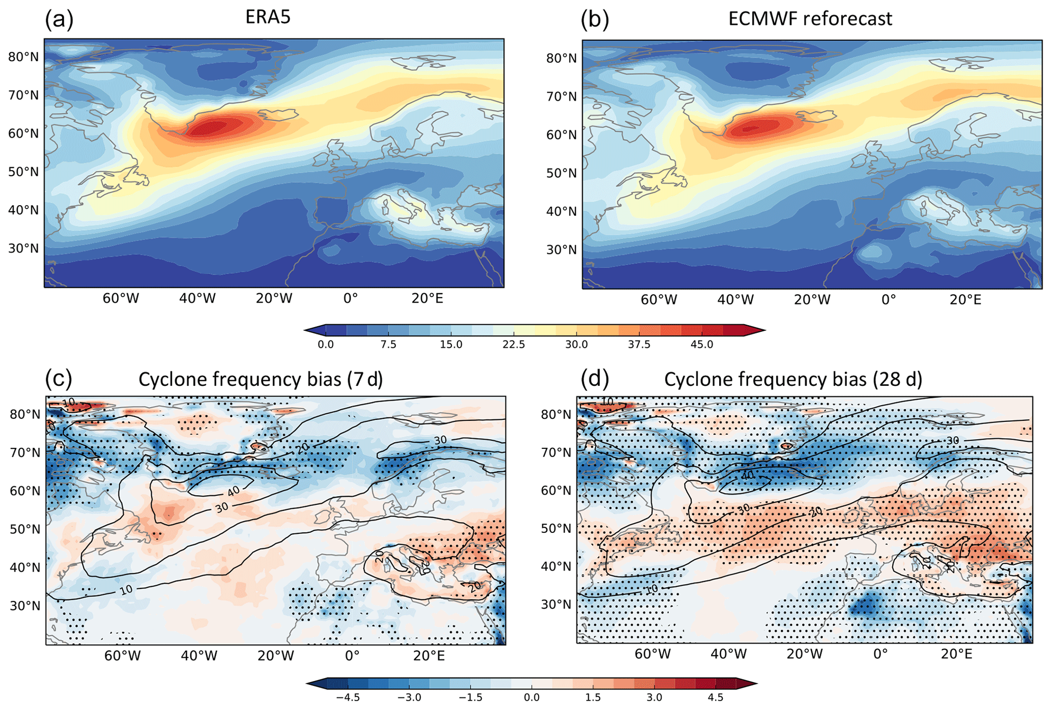
Figure 1Climatology of cyclone frequency (in %) for December to March (DJFM) in (a) ERA5 for the years 2000–2019 and in (b) ECMWF reforecasts for the same period. The climatology for the reforecasts is computed using all available initializations between 1 December and 1 March and averaged over a period of 28 d (days 1–28 with respect to the initialization date). (c) Model bias (shading, in %) according to the difference between ECMWF reforecasts and reanalysis (reforecast minus reanalysis) over a period of 7 d starting on the day of initialization, and (d) is the same as (c), but for a period of 28 d. Black contours in (c) and (d) show the climatological cyclone frequency in the reforecasts as shown in panel (b).
The spatial distribution of cyclone frequency is generally well represented in the reforecasts (Fig. 1b). Yet, the forecast system overestimates the cyclone frequency across midlatitudes between about 40–60∘ N (Fig. 1c and d), while it underestimates the cyclone frequency along the storm track maximum and north of 60∘ N. The signature of the midlatitude bias in cyclone frequency is significantly larger when computed for a period of 28 d starting on the day of initialization (Fig. 1d), compared to the biases over a period of 7 d (Fig. 1c).
These results demonstrate the general ability of the ECMWF forecast systems to reproduce the DJFM climatological storm track, although regional biases exist, particularly in the North Atlantic and over northern Europe, whose origin and consequences will have to be investigated further. A more in-depth analysis of subseasonal reforecast biases for Northern Hemisphere cyclone frequency and life cycle characteristics will be published in a separate future study.
3.2 Zonal wind response following SSW and strong polar vortex events
As a next step, we assess the prediction of the surface response following stratospheric extreme events on subseasonal timescales. We first analyze zonal wind anomalies at 850 hPa following stratospheric extreme events, focusing on the differences between SSW and strong polar vortex events.
Figure 2 shows a composite of 850 hPa zonal wind after SSW and strong polar vortex events in the ERA5 and the ECMWF reforecasts. Following SSW events, zonal wind anomalies in the reanalysis strengthen over the subtropical North Atlantic, particularly equatorward of 40∘ N, whereas a weakening of the zonal wind occurs in midlatitude, between 40–60∘ N in the North Atlantic (Fig. 2a). These changes correspond to an equatorward shift in the eddy-driven jet. A similar spatial pattern of the downward impact is found in the reforecasts; however, the maximum weakening occurs over a wider region in the reforecasts compared to the reanalysis, e.g., over the North Atlantic, as well as over the Baltic Sea and Scandinavia (Fig. 2c). Over the midlatitudes of the North Atlantic, as well as over the subtropical Atlantic, 850 hPa zonal wind anomalies are statistically significant. Note the difference in sample size between reanalysis and the reforecasts due to the ensemble size (although ensemble members are not independent of each other).
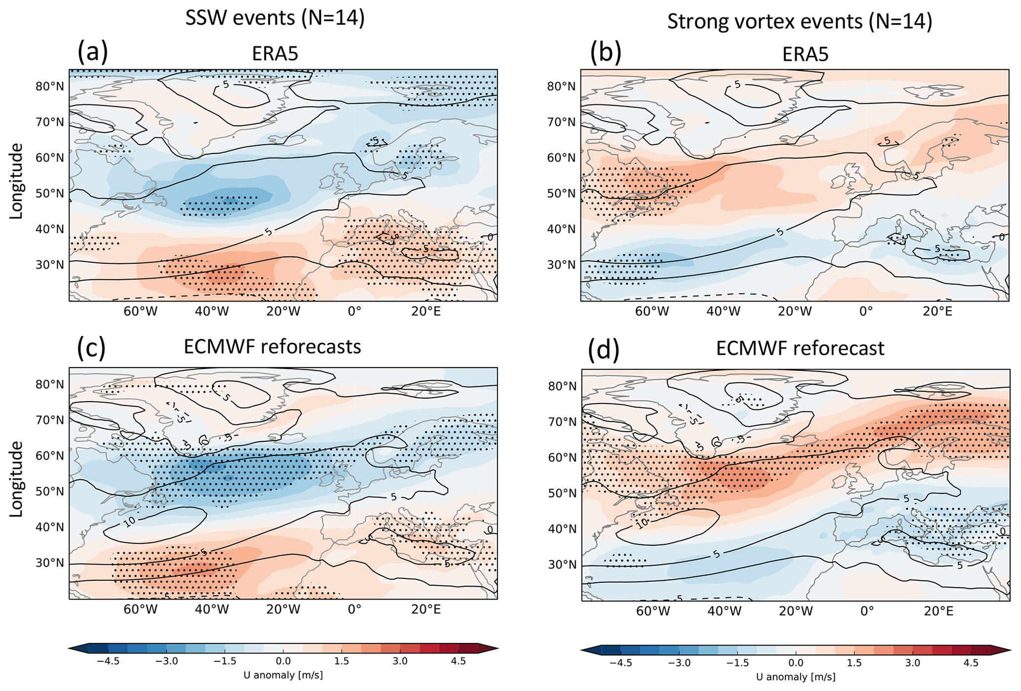
Figure 2Zonal wind anomalies at 850 hPa (color shading; in m s−1) following (left) sudden stratospheric warming (SSW) and (right) strong polar vortex events in (a, b) ERA5 following stratospheric extreme events and (c, d) ECMWF reforecasts initialized on the same date of the events or between 1 to 3 d after their first day and averaged over a period of 28 d starting on the day of initialization. ERA5 and the reforecasts are averaged over the same period. Black contours in each panel show the 850 hPa zonal wind climatology for DJFM of the respective dataset. Anomalies statistically significant at the 90 % confidence level based on Student's t test are indicated by the hatching.
In contrast to SSW events, 850 hPa zonal wind anomalies after strong polar vortex events show a strengthening over middle and high latitudes in the North Atlantic in the reanalysis, while a weakening of the wind occurs more equatorward, in the subtropical North Atlantic (Fig. 2b). A similar pattern is observed in the reforecasts, with a significant increase in zonal wind anomalies over in middle and high latitudes compared to the reanalysis (Fig. 2d). These changes coincide with a poleward jet shift in the North Atlantic region.
3.3 Cyclone frequency response following SSW and strong polar vortex events
After SSW events, the North Atlantic storm track in reanalysis strengthens on its southern flank relative to its climatological position and extends further into Europe (red box in Fig. 3a). This response of the North Atlantic storm track is consistent with the change in the North Atlantic jet stream, which also strengthens on its southern flank after SSWs (Fig. 2a). Over northern Europe, the cyclone frequency response is found to be stronger in reanalysis (Fig. 3a) compared to the reforecasts (red box in Fig. 3c).
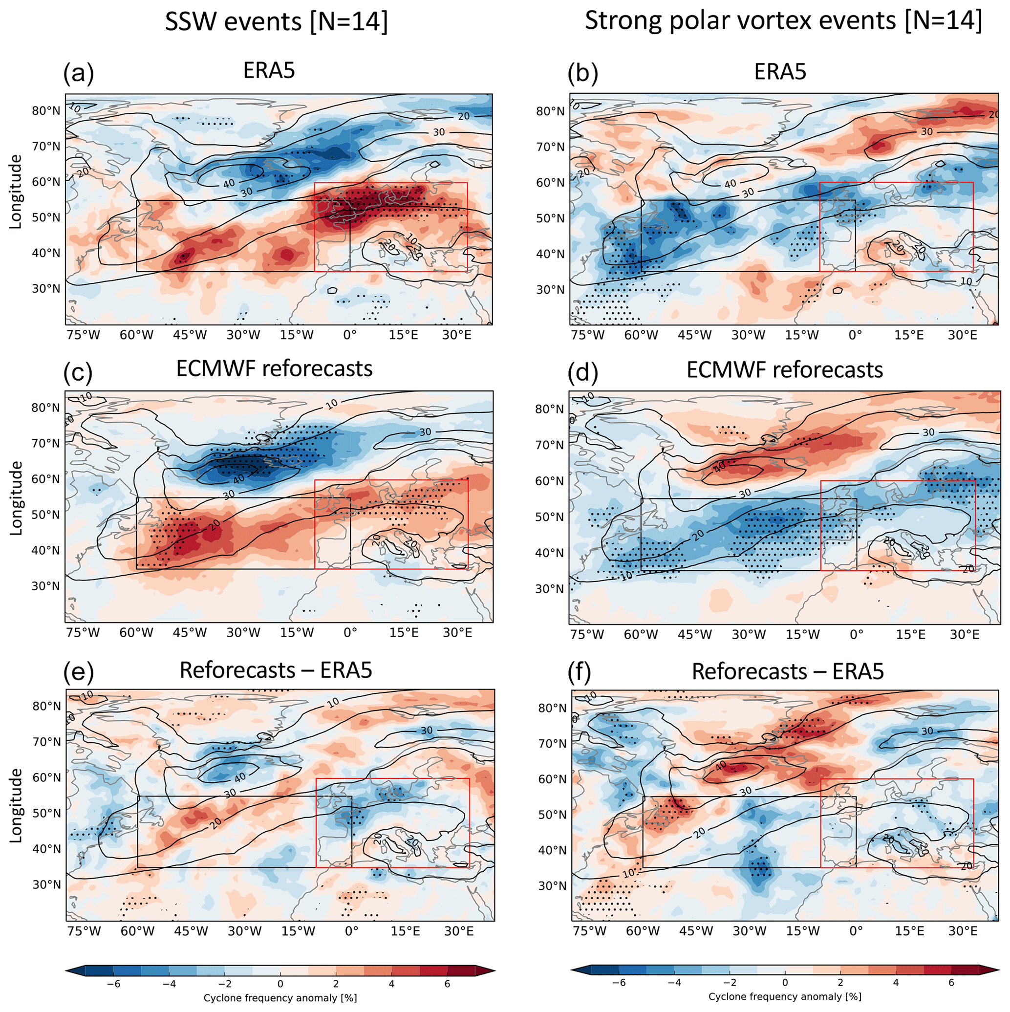
Figure 3Same as Fig. 2, but for cyclone frequency anomalies (in %). Reforecasts are initialized on the same date of stratospheric extreme events or between 1 to 3 d after their first day and averaged over a period of 28 d. ERA5 is averaged over the same dates. (e, f) Differences in cyclone frequency anomalies between reforecasts and reanalysis following (e) SSW and (f) strong polar vortex events. Black contours show the climatological cyclone frequency in reforecasts for DJFM. Anomalies statistically significant at the 95 % confidence level based on Student's t test are indicated by the hatching.
Consistent with the zonal wind response, cyclone frequency in the strong polar vortex composite is enhanced over high latitudes in the North Atlantic (particularly 60–70∘ N) both in the reanalysis and in the model (Fig. 3b and d). The maximum strengthening, however, occurs more northeastward in the reanalysis (e.g., over the Norwegian and Barents seas; Fig. 3b) compared to the reforecasts, where most of the strengthening is between Greenland and Iceland (Fig. 3d). Both the reanalysis and the reforecasts show a significantly reduced cyclone frequency over the central North Atlantic (particularly between 35 to 55∘ N) (black box in Fig. 3b and d).
Figure 3e and f show the difference in cyclone frequency anomalies between reforecasts and reanalysis after SSW (Fig. 3e) and strong polar vortex (Fig. 3f) events. After SSWs, the model overestimates cyclone frequency over the central North Atlantic compared to the reanalysis, particularly between 40 and 50∘ N and over the Norwegian Sea (Fig. 3e). At higher latitudes, particularly south of Greenland, the reforecasts overestimate the reduction in cyclone frequency after SSW events compared to the reanalysis.
Overestimation of cyclone frequency anomalies in the reforecasts in comparison with reanalysis also occurs at higher latitudes (particularly between 60 to 70∘ N) after strong polar vortex events (Fig. 3f), with statistically significant anomalies along the tilted storm track maximum. Over the central Atlantic the reforecasts underestimate the cyclone frequency relative to the reanalysis.
The regional aspects of the cyclone frequency response after stratospheric extreme events can be more clearly characterized by analyzing the changes in cyclone frequency anomalies over specific regions after extreme stratospheric events. One of the surface impacts of SSW events is the occurrence of anomalously wet conditions over western Europe and the Mediterranean and anomalously dry conditions over Scandinavia (e.g., Butler et al., 2017). These changes in precipitation patterns are likely linked to the cyclone frequency over these regions. Hence, in the next subsections we examine whether cyclone frequency after SSW events is indeed increased over the central and southern Atlantic region, and decreased in more poleward regions. For this purpose, we focus our analysis on the midlatitude region (35–55∘ N) of the North Atlantic (60∘ W–0∘ E) and over Europe (35–60∘ N, 10∘ W–33∘ E). These regions, located on the southern flank of the North Atlantic storm track, are where the change in cyclone frequency after SSW and strong polar vortex events is the largest (black and red boxes in Fig. 3, respectively).
3.4 Cyclone life cycle characteristics following SSW and strong polar vortex events
We now investigate how the average cyclone life cycle characteristics depend on the extreme states of the stratospheric polar vortex at forecast initialization. More specifically, we analyze the spatial propagation and intensity characteristics of individual cyclone tracks, which have been identified based on an objective tracking algorithm (see Sect. 2.2 for details). Figure 4 shows all cyclone tracks in ERA5 and in the reforecasts during the 28 d following SSW and strong polar vortex events. There are more tracks shown for the reforecasts than for reanalysis due to the use of all available ensemble members (11 members in each reforecast). Independent of the stratospheric state, the highest track densities can be found in the climatological hotspot regions along the US east coast and south of Greenland (see black contours in Fig. 4e and f, which show the DJFM climatological cyclone frequency), while fewer cyclones are present over Europe and the Mediterranean. Focusing on the median track (red and blue lines, corresponding to SSW and strong polar vortex events, respectively), however, reveals a slight equatorward shift in the average cyclone propagation after SSWs, particularly over the eastern half of the North Atlantic and over Europe, which is largely in line with the findings of Baldwin and Dunkerton (2001, see their Fig. 5). However, this shift is only significant (i.e., the two confidence intervals do not overlap; see caption of Fig. 4 for details) in the reforecasts (Fig. 4f) but not in ERA5 (Fig. 4e), which might partly be related to the smaller sample size in ERA5.
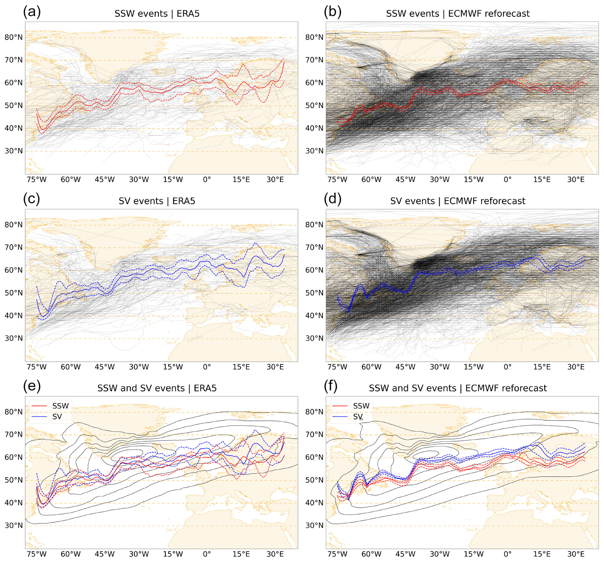
Figure 4Statistics of individual cyclone tracks with a lifetime of at least 24 h and a maximum intensity of at least 990 hPa reached within the North Atlantic–European domain in ERA5 (a, c, e) and in the reforecasts (b, d, f). The individual tracks occurring within 28 d after the SSW and strong polar vortex (SVs) events are shown in black (a–d), and the corresponding median latitude (solid) of all tracks in 1∘ longitudinal bands and its 90 % confidence interval (dashed) are shown in red and blue. The confidence interval is obtained from a bootstrapped distribution of median latitudes (based on 1000 random resamples of the tracks with replacement). The DJFM cyclone frequency climatology is shown as black contours in (e) and (f).
We further investigate how extratropical cyclones following SSW and strong polar vortex events differ in terms of intensity as an important metric for surface impacts. The cyclones following strong polar vortex events tend to reach higher maximum intensities (i.e., lower sea level pressure) than the cyclones following SSW events in both ERA5 and in the reforecasts, as the shift between the red (SSW) and blue (strong polar vortex) distributions in the upper left panels of Fig. 5a and b indicates. To determine whether these differences are significant, we split the SSW and strong polar vortex distributions into 1 % sized percentile bins, compute the difference between the percentile values of the SSW and strong polar vortex distributions for each of these bins (black line in bottom left panels of Fig. 5a and b), and check whether this difference is outside the corresponding 99.9 % confidence interval (gray shading; see caption of Fig. 5a and b for how the confidence interval is computed). According to this analysis, the difference in intensities following SSW and strong polar vortex events is highly significant in the reforecasts but not significant in ERA5, which, however, might again be related to the smaller sample size in ERA5. To some degree, the higher intensities might be explained by the fact that the more northern cyclones following strong polar vortex events (see Fig. 4e and f) are located in regions with climatologically lower sea level pressure. Nevertheless, cyclones following strong polar vortex events also tend to experience higher maximum intensification rates (upper right panels of Fig. 5a and b). These stronger intensification rates might be linked to the larger poleward component of the cyclones' propagation direction, as well as the stronger North Atlantic jet following strong polar vortex events (Fig. 2), which both correlate with cyclone intensification (e.g., Rivière et al., 2012; Tamarin and Kaspi, 2016; Besson et al., 2021). However, the differences in maximum intensification between SSW and strong polar vortex events are not significant in ERA5 and only significant for the most strongly intensifying cyclones (i.e., the lower percentiles) in the reforecasts (bottom right panels of Fig. 5a and b).
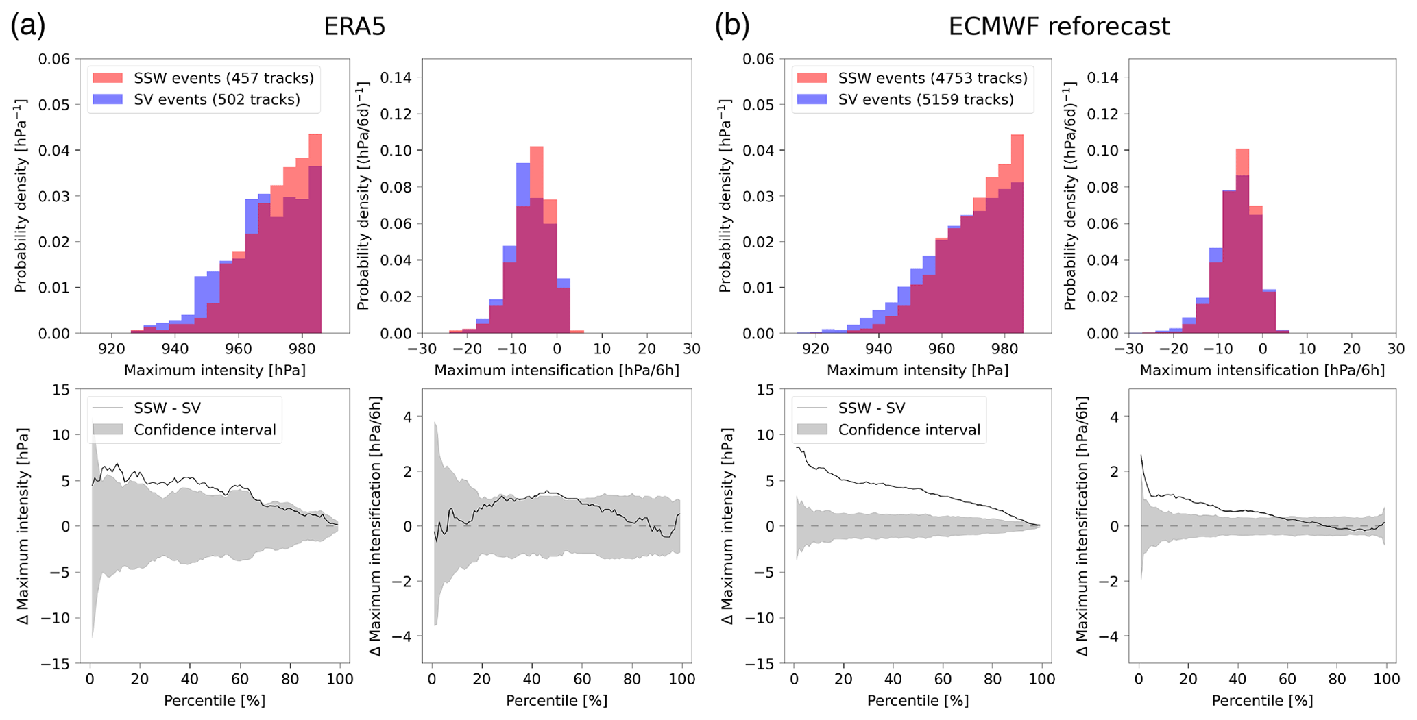
Figure 5Frequency histograms for maximum intensity (defined as the lowest sea level pressure minimum along the track) and maximum 6-hourly intensification along the track of the cyclones occurring within 28 d after the SSW (red) and strong polar vortex events (blue) in ERA5, and the reforecasts are shown in the first row. The corresponding differences between the percentile values of the SSW and strong polar vortex distributions are shown by the black lines in the second row (see text for details), complemented by their 99.9 % confidence intervals in gray. The confidence intervals are obtained as follows: all data points of both the reforecasts and ERA5 are combined into one distribution, and this distribution is randomly shuffled. The shuffled distribution is then split into two new equally sized distributions mimicking the “ERA5” and “reforecast” distributions, and the percentile-wise difference between these two random distributions is computed in the same way as for the original distribution. This procedure is repeated 10 000 times to obtain a distribution of differences for each 1 % sized percentile bin.
3.5 Reforecast performance for regional cyclone frequency after SSW and strong polar vortex events
Next, the ability of the subseasonal ensemble reforecasts in predicting North Atlantic cyclone frequency after SSW or strong polar vortex events is examined (Fig. 6). We focus on two sectors: the central region of the North Atlantic (35–55∘ N, 60∘ W–0∘ E; black box in Fig. 3) and Europe (35–60∘ N, 10∘ W–33∘ E; red box), where anomalous cyclone frequencies are expected following SSW and strong polar vortex events (see Fig. 3). Red bars in Fig. 6a indicate the proportion of ensemble members that show an average increase in cyclone frequency over this region, whereas blue bars indicate a decrease. For simplicity, 10 ensemble members (i.e., 10 perturbed simulations of the forecast system, excluding the control run) are analyzed for each event.
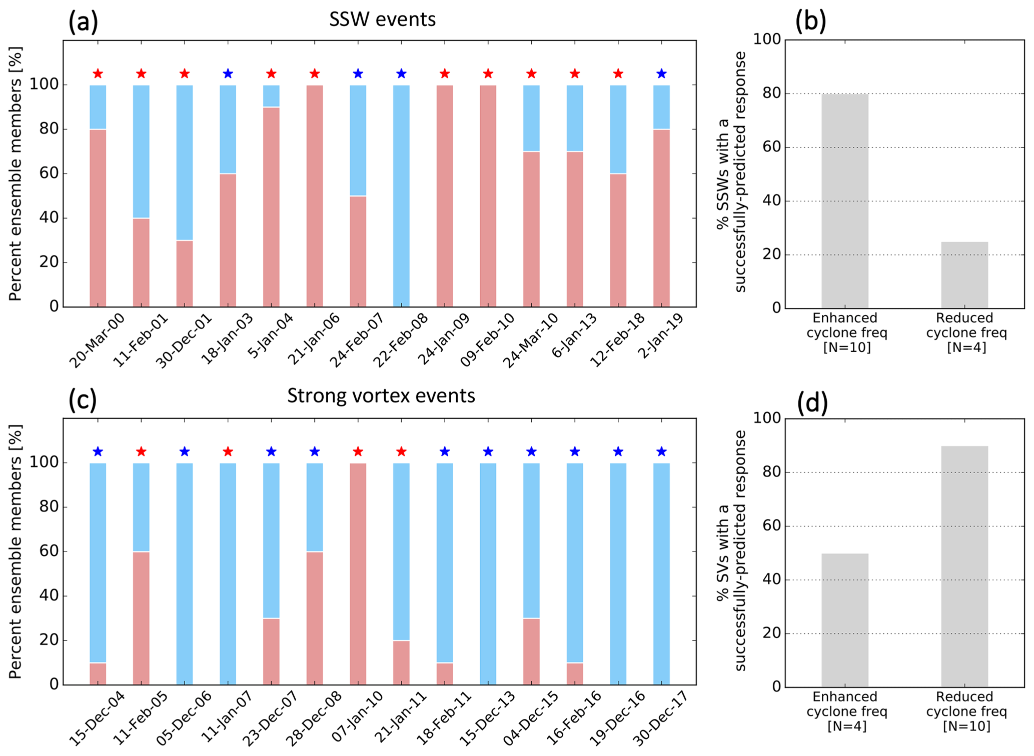
Figure 6(a, c) Bars represent the percentage of ensemble members that predict an enhancement (red) or a reduction (blue) of cyclone frequency anomaly over the central North Atlantic (35–55∘ N, 60∘ W–0∘ E; black box in Fig. 3a) after (a) SSW and (c) strong polar vortex events (SVs) in the ECMWF reforecasts. The x axis in (a, c) indicates the central dates of the stratospheric events. Anomalies are averaged over days 1–28 of the reforecast. Red and blue asterisks indicate the average response based on ERA5, with red (blue) indicating an increase (decrease) of cyclone frequency anomaly over this region. (b, d) The percentage of events where more than 50 % of the ensemble members predict the correct sign of the cyclone frequency anomaly over the midlatitude North Atlantic region for (b) SSW and (d) strong polar vortex events.
3.5.1 North Atlantic
The majority of SSW events are followed by an enhancement of cyclone frequency in the central North Atlantic in the reanalysis (10 out of 14 events) as indicated by the red stars in Fig. 6a. The cyclone frequency response following these events is generally well predicted, with an increase in cyclone frequency predicted by more than 60 % of the ensemble members in the reforecasts (Fig. 6a). In contrast, the response after SSW events with a decrease in cyclone frequency over the central Atlantic tends to be less predictable, with the majority of ensemble members predicting a decrease in only one out of four SSW events (Fig. 6a).
Strong polar vortex events, on the other hand, tend to be followed by a decrease in cyclone frequency in the reanalysis (10 out of 14 events, indicated by the blue stars in Fig. 6c). This response is generally captured well by the reforecasts, with 60 % or more of the ensemble members predicting a reduction in cyclone frequency after strong vortex events (Fig. 6c).
On average over all events, about 60 % of ensemble members predict a positive sign of the cyclone frequency anomaly in the central Atlantic after SSW events, compared to 40 % of ensemble members predicting a negative anomaly. The opposite ratio between ensemble members with an enhanced versus reduced cyclone frequency response is found after strong polar vortex events. For SSWs, this ratio corresponds to the percentage of SSW events with a canonical downward response, i.e., an equatorward shift in the North Atlantic jet (e.g., Afargan-Gerstman and Domeisen, 2020).
Another way to evaluate the model performance in predicting anomalies of cyclone frequency is by computing the percentage of hits for SSW and strong polar vortex events (Fig. 6b and d). A hit is defined when more than 50 % of the ensemble members predict the correct sign (i.e., the same as in reanalysis) of the cyclone frequency anomaly over the selected region.
Overall, we find that the majority of SSW events with an enhanced cyclone frequency response in the midlatitude Atlantic are well predicted (80 % of SSWs) in terms of the sign of their downward impact, compared to only 25 % of SSW events with a reduced cyclone frequency response (Fig. 6b). For comparison, strong polar vortex events tend to have higher success rates than SSWs, with more than 70 % of strong polar vortex events having a successfully predicted cyclone frequency response (Fig. 6d). These success rates are found for strong polar vortex events with both an enhanced or reduced response.
3.5.2 Europe
Similar to the North Atlantic, we find that the majority of SSW events are followed by an enhancement of cyclone frequency over Europe in the reanalysis (12 out of 14 events; Fig. 7a), whereas strong polar vortex events are generally followed by a decrease in cyclone frequency over Europe (8 out of 14 events; Fig. 7b). However, the number of strong vortex events with a reduced cyclone frequency response is lower over Europe compared to the North Atlantic (8 versus 10 events). In terms of the percentage of hits, SSW events with an enhanced cyclone frequency response over Europe are found to be well predicted (80 % of SSWs), compared to only 50 % of SSW events with a reduced cyclone frequency response (Fig. 7b). This ratio is higher over Europe compared to the North Atlantic (Fig. 6b), where only 25 % of SSW events with a reduced cyclone frequency response are successfully predicted (however, the number of events with such a response is larger).
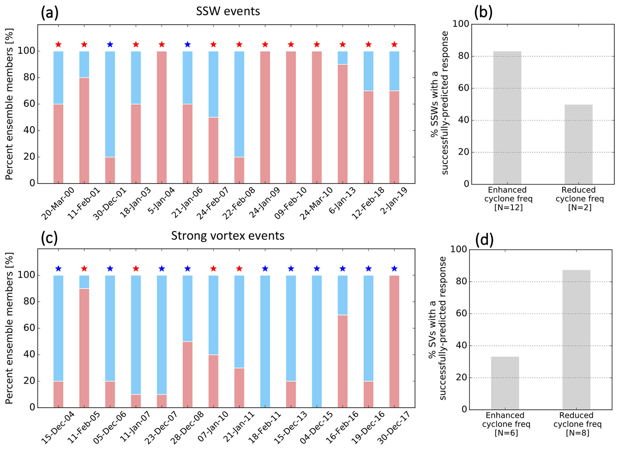
Strong polar vortex events, on the other hand, exhibit a high number of hits compared to SSWs over the European region, with more than 90 % of strong polar vortex events having a successfully predicted reduced cyclone frequency response (Fig. 7d). Success rates, however, are lower over Europe compared to the North Atlantic for strong polar vortex events with enhanced cyclone frequency response (30 % of strong vortex events over Europe, compared to 50 % over the North Atlantic). Overall, these differences in predictability over Europe compared to the North Atlantic suggest that SSWs are characterized by higher success rates over Europe, for both enhanced and reduced cyclone response.
3.6 Evaluation of cyclone frequency prediction on weekly timescales
Next, in order to better understand the time evolution of the cyclone frequency response to stratospheric influences, we evaluate the hits for each week separately, starting from the central date of the SSW or strong polar vortex event (Fig. 8). For the majority of SSW events, the percentage of hits is lower in weeks 3–4 compared to weeks 1–2 (Fig. 8a). Out of 14 SSW events, several events have a low hit rate even in week 1 (e.g., 20 March 2000, 5 January 2004, 24 March 2010). Strong polar vortex events, on the other hand, are followed by a high hit rate for week 1, with a 100 % hit rate for most strong polar vortex events (Fig. 8b). The hit rate rapidly drops in the subsequent weeks.
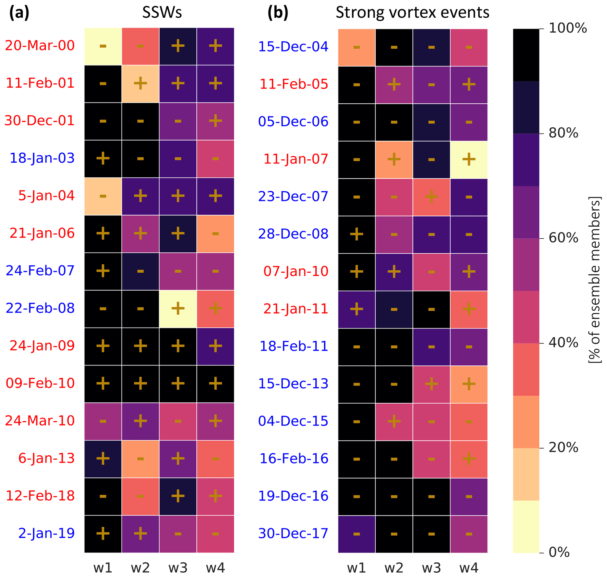
Figure 8Percentage of ensemble members that predict the observed cyclone frequency response over the central North Atlantic (35–55∘ N, 60∘ W–0∘ E) after (a) SSW and (b) strong polar vortex events in the ECMWF reforecasts. Anomalies are averaged for every week in the reforecast (w1 is between days 1–7, w2 between days 8–14, etc.) with respect to the central date of the event. For each week, the observed response is indicated by a “+” (“−”) sign corresponding to an increase (decrease) of cyclone frequency anomaly in the selected region. A red (blue) date corresponds to an average increase (decrease) of cyclone frequency anomaly during weeks 1–4.
These differences between SSW and strong polar vortex events again suggest that the model may encounter more challenges in predicting the cyclone frequency response after SSW events compared to strong polar vortex events. The reasons for this behavior can vary between the events: for example, the SSW event of 22 February 2008 was followed by a reduction in cyclone frequency over the central Atlantic (as indicated by the red star in Fig. 6a); while the forecast model prediction is in good agreement with observations for weeks 1 and 2 (Fig. 8a), none of the ensemble members predicted the observed cyclone frequency response in week 3, and the hit rate remained relatively low in the following week.
Overall, this analysis shows that while 70 % of the reforecasts capture the sign of the cyclone frequency response over the North Atlantic during weeks 1–2 after SSWs, less than 50 % of the reforecasts capture the response during weeks 3–4. The cyclone forecasts following strong polar vortex events are generally more successful, with around 80 % of the reforecasts predicting the response during week 1 and around 60 % capturing the response in the following weeks.
3.7 Dynamical aspects of successful and unsuccessful predictions
Here, the relationship between ensemble members predicting the observed cyclone frequency response after SSW and strong polar vortex events and the large-scale atmospheric circulation patterns at the surface and in the lower stratosphere is examined. We use 850 hPa zonal wind (U'850) and geopotential height anomalies at 100 hPa (Z'100) in the aftermath of the stratospheric events to evaluate the predictions.
Figure 9 shows the time evolution of the cyclone frequency prediction averaged over the North Atlantic (60∘ W–0∘ E) after SSW and strong vortex events (Fig. 9a and b, respectively). Only events with a canonical downward response (according to the reanalysis) are used: SSW events with an enhanced cyclone frequency in the midlatitude North Atlantic and strong polar vortex events with a reduced cyclone frequency in the same region.
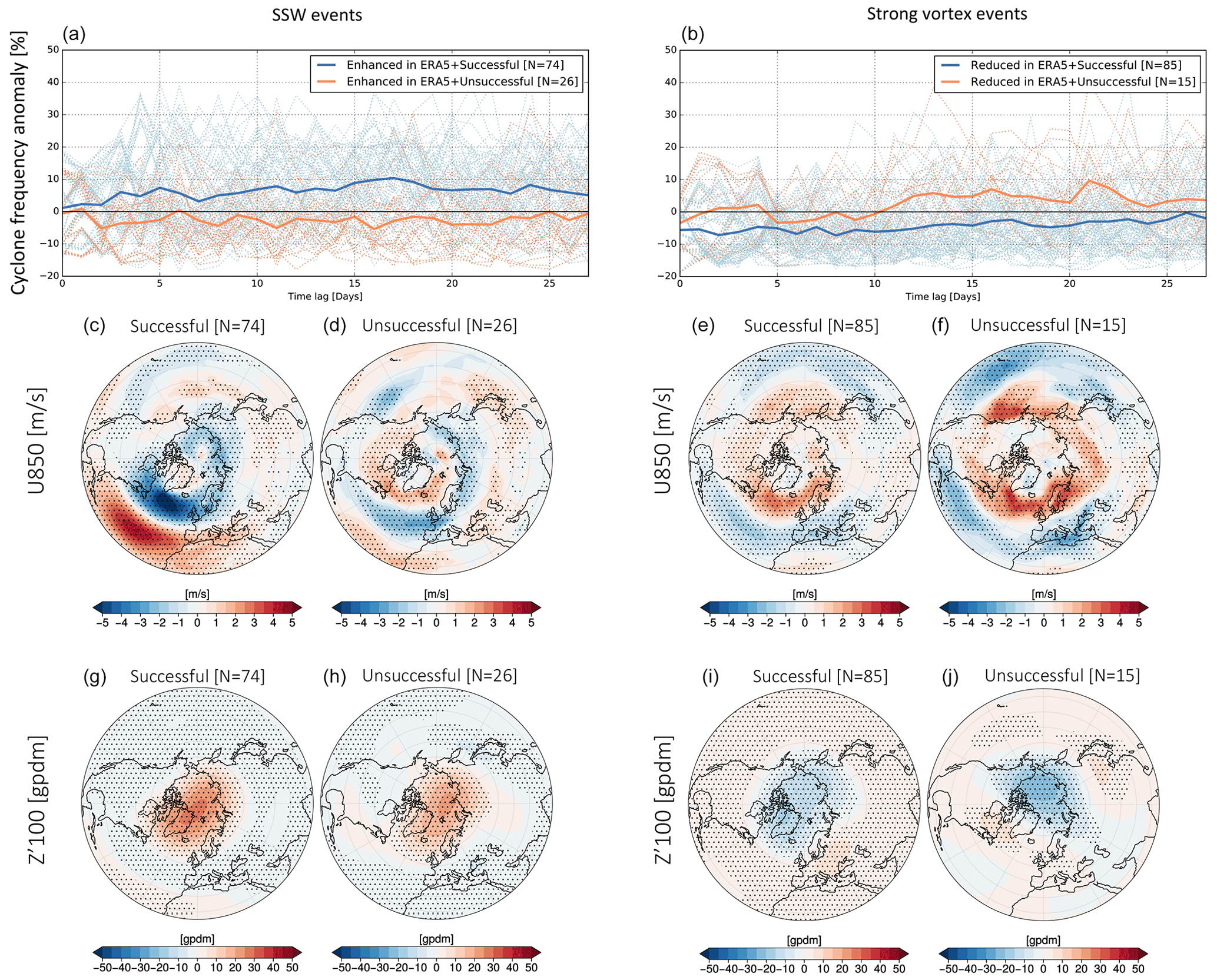
Figure 9(a, b) Time evolution of cyclone frequency anomaly (in %), zonally averaged over the midlatitude North Atlantic, following (a) SSW events and (b) strong polar vortex events with a canonical surface response (see text for definition). Ensemble members with a successful (blue) and unsuccessful (orange) prediction of cyclone frequency are highlighted. The bold line is the ensemble mean of each composite. The numbers in the brackets of the legend show the number of events in each composite. (c–f) Composites averaged over 28 d of 850 hPa zonal wind anomalies (in m s−1) for (c, e) successful and (d, f) unsuccessful prediction after SSW and strong polar vortex events, respectively. (g–j) Same as (c–f), but for geopotential height anomalies of the 100 hPa surface (Z'100; in gpdm). Anomalies statistically significant at the 90 % confidence level based on Student's t test are indicated by the stippling.
For each reforecast, the ensemble members are separated into two subgroups according to the success of their prediction. A successful prediction (indicated by the blue curves in Fig. 9a and b) is defined here per ensemble member that predicts the observed sign of the cyclone frequency anomaly in the North Atlantic (based on a 28 d average of the response after the onset of SSW or strong vortex events, respectively). In contrast, unsuccessful predictions (indicated by the orange curves in Fig. 9a and b) are defined as members that do not predict the observed sign on the response for the same period.
We find that out of 100 ensemble members of SSW events with a canonical surface response (i.e., enhanced cyclone frequency in the midlatitude North Atlantic), 74 % successfully predict the sign of the downward response, whereas 26 % are unsuccessful in predicting the correct sign. For strong polar vortex events with a canonical surface response (i.e., reduced cyclone frequency in the midlatitude North Atlantic), 85 % out of 100 ensemble members result in a successful prediction and 15 % in an unsuccessful prediction. Furthermore, we find that cyclone frequency anomalies in unsuccessful predictions diverge from the successful forecasts within the first 2–4 d with respect to the central date.
Lower-tropospheric zonal wind anomalies at 850 hPa for successful and unsuccessful predictions of the cyclone frequency response in the North Atlantic after SSW and strong vortex events are shown in Fig. 9c and d and e and f, respectively. As expected, SSW events with a successful canonical response are characterized by negative U'850 anomalies poleward of 45∘ N and positive U'850 anomalies more equatorward, consistent with an equatorward jet shift in this region (Fig. 9c). The unsuccessful predictions, however, are characterized by a weakening of the zonal wind in the central North Atlantic, as well as in southern and central Europe (Fig. 9d). For strong polar vortex events, strengthening of the North Atlantic jet poleward of 45∘ N is consistent with a poleward jet shift in both successful and unsuccessful predictions of the surface response.
Anomalies of Z'100 are found to be positive over the polar cap after SSW events (Fig. 9g and h), and negative anomalies are found after strong vortex events (Fig. 9i and j) in both successful and unsuccessful predictions. For SSW events, positive polar cap anomalies of Z'100 are found to be stronger for SSWs with a successful prediction, compared to the unsuccessful predictions, consistent with previous studies on the importance of lower-stratospheric geopotential height anomalies for the downward impact (e.g., Karpechko et al., 2017; Afargan-Gerstman et al., 2022). For the strong polar vortex events, however, negative geopotential height anomalies over the polar cap are found to have a more zonally symmetric pattern at 100 hPa in the case of a successful prediction (Fig. 9i) and a more asymmetric pattern for unsuccessful predictions (Fig. 9j).
Thus, we find that ensemble members with a successful prediction of the canonical downward influence in the Atlantic differ from unsuccessful members mostly in their representation of tropospheric circulation anomalies after SSW events, indicating that the troposphere plays a dominant role in a successful prediction of the downward impact of stratospheric anomalies after SSW events, as, for example, indicated by Domeisen et al. (2020b). Following strong polar vortex events, however, members with successful predictions differ from unsuccessful members in both their tropospheric and lower-stratospheric anomalies.
To further understand the difference in tropospheric circulation between successful and unsuccessful predictions of the cyclone frequency response, we analyze the time evolution of zonal wind and geopotential height anomalies for successful and unsuccessful predictions after SSW and strong vortex events (Figs. 10 and 11, respectively). Anomalies are plotted for every week in the reforecast with respect to the central date of the event.
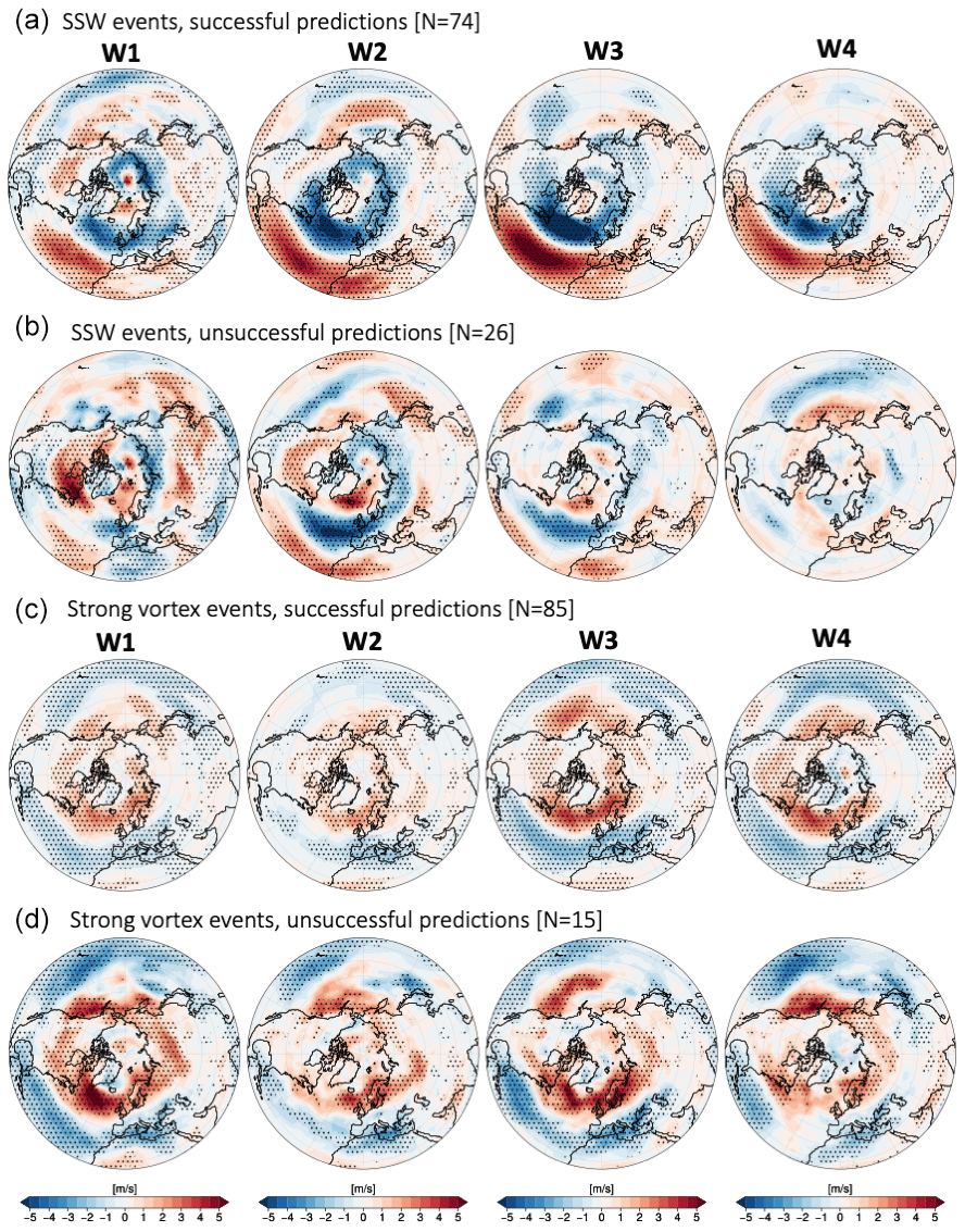
Figure 10Same as panels (c–j) in Fig. 9, but for U'850 anomalies in every week in the reforecast (w1 is between days 1–7, w2 between days 8–14, etc.) with respect to the central date of the event. Anomalies are shown for (a, c) successful and (b, d) unsuccessful predictions after SSW and strong polar vortex events, respectively.
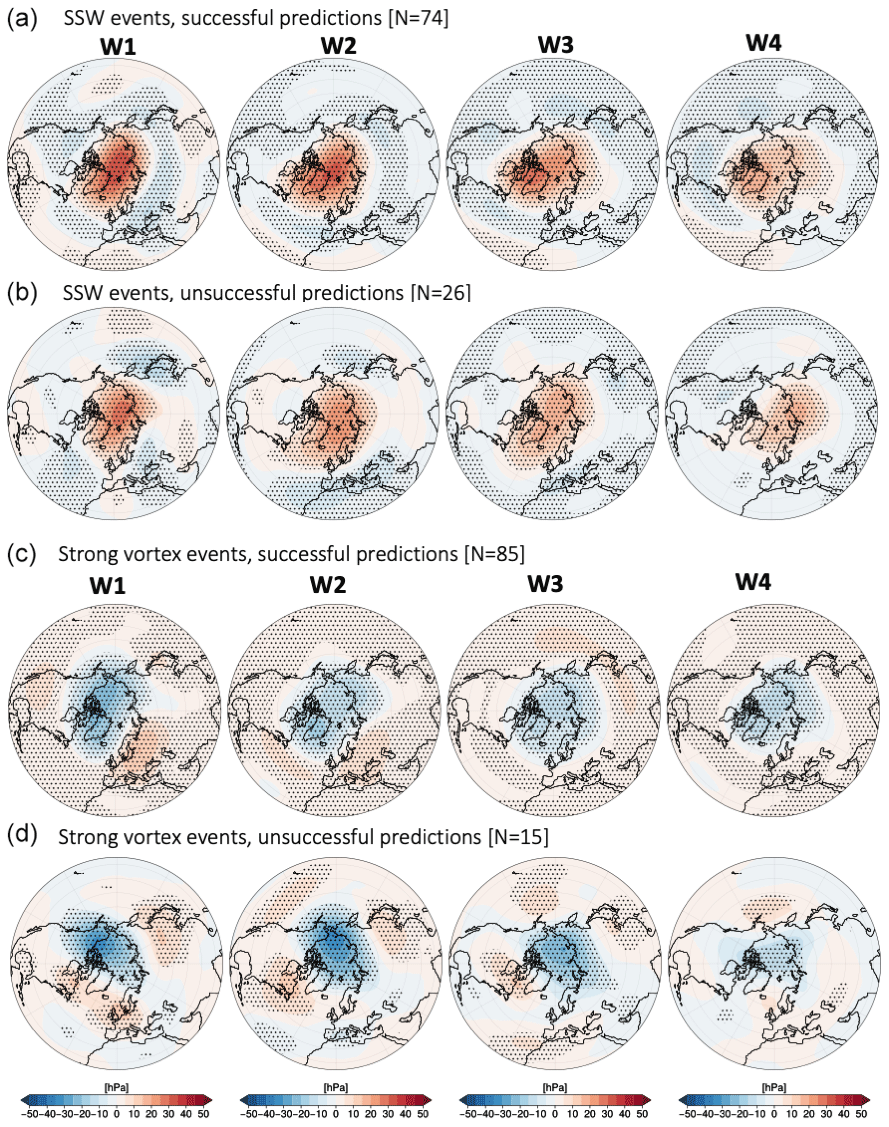
Figure 11Same as Fig. 10, but for Z'100 for (a, c) successful and (b, d) unsuccessful predictions after SSW and strong polar vortex events, respectively.
Successful predictions of the canonical downward impact after SSW events are found to be associated with a persistent equatorward shift in the North Atlantic jet between week 1 and week 4, as shown by the zonal wind anomalies at 850 hPa (Fig. 10a), while unsuccessful predictions show a persistent pattern only during weeks 2 and 3 (Fig. 10b). In contrast to SSW events, both successful and unsuccessful predictions of the canonical impact after strong polar vortex events exhibit a persistent response between week 1 and week 4, particularly after week 3 (Fig. 10c and d).
For comparison, successful predictions of the canonical downward impact are characterized by positive Z'100 anomalies over the polar cap in weeks 1 to 4 and a similar but weaker pattern of polar cap Z'100 anomalies in unsuccessful predictions (Fig. 11a and b). On the other hand, strong polar vortex events are followed by a negative pattern of Z'100. Unsuccessful predictions exhibit larger variability in the surface circulation compared to successful predictions, with a zonally asymmetric anomalous Z'100 pattern in every week of the reforecast (Fig. 11c and d).
Figure 12 shows the time evolution of the ensemble mean prediction for cyclone frequency anomaly (Fig. 12a and b) averaged over the North Atlantic (60∘ W–0∘ E) for SSW and strong vortex events, respectively. All reforecasts are initialized after the onset of the events (see Sect. 2.3 for details). The ensemble mean is computed for each event separately and then averaged over all selected events.
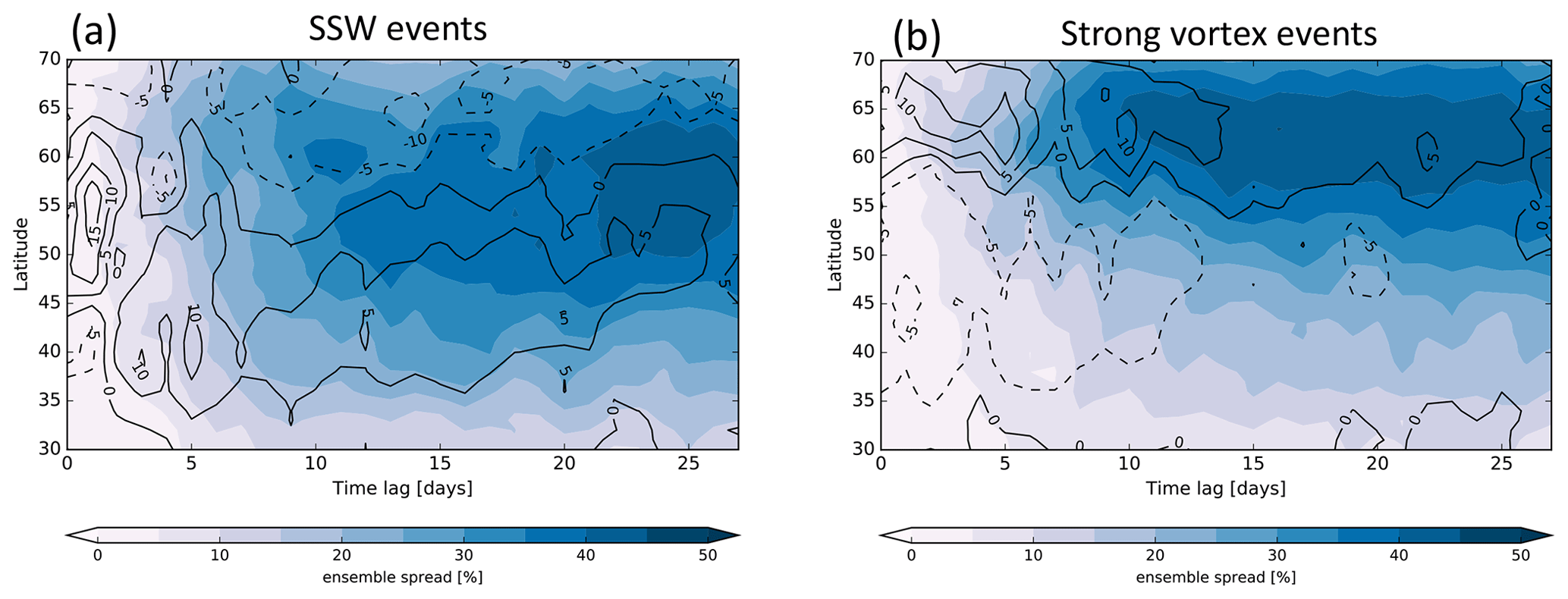
Figure 12Ensemble mean prediction (black contours; negative values are dashed) and ensemble spread (color shading) for zonal mean cyclone frequency anomaly (in %), averaged over the North Atlantic (60∘ W–0∘ E) for reforecasts initialized after (a) SSW and (b) strong polar vortex events. Only events with a canonical surface response in the reanalysis are included in the composites.
The ensemble mean shows the enhancement of cyclone frequency in the midlatitudes after SSW events (solid contours in Fig. 12a). After initialization, cyclone frequency is increased between 45 to 60∘ N. Starting from day 5, positive anomalies are observed further equatorward (mostly between 30 to 55∘ N), consistent with an equatorward shift in the storm track. On the other hand, ensemble predictions after strong vortex events show a decrease in cyclone frequency in the midlatitude region (30 to 55∘ N), starting at day 0 (dashed contours in Fig. 12b), indicative of an average poleward shift in the storm track in this region.
Next, we examine the ensemble spread for these reforecasts. The ensemble spread is represented by the standard deviation with respect to the ensemble mean. As for the ensemble mean, the ensemble spread shown in Fig. 12 is averaged over all events with a canonical downward response. Reforecasts after SSWs exhibit a relatively small spread in the first days after the onset of the SSW events; however, the spread increases gradually with time, in particular after day 10 (Fig. 12a). An additional increase in ensemble spread occurs after day 20. Throughout its evolution, the spread is largest between 45 and 60∘ N, which marks the transition zone between positive and negative cyclone frequency anomalies after SSW events. Interestingly, the ensemble spread after strong vortex events is largest at high latitudes, between 55 and 70∘ N (Fig. 12b), which is the region corresponding to the poleward shift in the ensemble mean.
Overall, the largest spread is found between 50 and 65∘ N for SSW events and between 60 and 65∘ N for strong vortex events. While SSW and strong vortex events generally exhibit a similar but opposite tropospheric response, differences in the predictability of their response can be found, as shown by the ensemble spread beyond 10 d.
Our results show that stratospheric extremes can have a clear impact on the storm track and on cyclone occurrence and tracks, with clear differences between weak and strong stratospheric polar vortex events. In more detail, our results can be summarized as follows:
-
The subseasonal forecasts show the expected response of the North Atlantic jet stream following stratospheric extreme events (i.e., an equatorward shift after SSW events and a poleward shift after strong polar vortex events) when averaging over all events.
-
The North Atlantic storm track (measured by the local frequency of cyclone occurrence) exhibits a behavior consistent with the jet, i.e., an enhanced cyclone frequency equatorward of the climatological storm track maximum after SSW, and a reduced frequency after strong polar vortex events.
-
The strongest biases in the cyclone frequency model response are observed over northwestern Europe after SSW events, where cyclone frequency is underestimated, and after strong polar vortex events to the south and east of Greenland, where cyclone frequency is overestimated.
-
The southward shift after SSWs compared to strong polar vortex events also manifests itself over the eastern North Atlantic when defining the storm track by the median of individual cyclone tracks. Furthermore, the cyclones after strong polar vortex events intensify more strongly and reach higher intensities than after SSW events. However, both the differences in cyclone track location and cyclone intensity are only significant in the reforecasts but not in the reanalysis (with the exception of the significantly stronger cyclone intensities following strong polar vortex events also in reanalysis). A larger sample size would be required to determine whether this result is simply due to the smaller sample size in ERA5 or whether this might indicate a slight overconfidence of the reforecasts in predicting the storm track response.
-
For individual events, the sign of a canonical (expected) response, i.e., an enhancement in cyclone frequency in the central North Atlantic after SSWs and a reduction after strong polar vortex events, is generally well predicted (above 80 % of all events).
-
For SSW and strong polar vortex events without a canonical response, an enhanced cyclone frequency in the midlatitude North Atlantic is well predicted in 50 % of all strong polar vortex events, while a reduced cyclone frequency response is predicted only in 25 % of all SSW events.
-
SSWs exhibit significantly more variability between events with respect to predictability. In particular, the surface response to strong polar vortex events can almost always be predicted in the first lead week, with a decrease in predictability thereafter, while the predictability behavior for SSW events is much less uniform between events.
-
A successful prediction of the canonical response depends more strongly on a correct representation of the state of the troposphere than the lower stratosphere at the time of the SSW event, while for strong vortex events both the lower stratosphere and the surface state are important.
Concluding, the model successfully represents the surface cyclone frequency response after most strong polar vortex events, especially for short lead times. For SSW events, however, the results are more mixed: the model is generally more successful in predicting the cyclone frequency after SSWs when the response to the stratospheric events exhibits the canonical response, i.e., an equatorward shift in the storm track. This result points towards a possible overconfidence of the model with respect to reanalysis to predict the canonical response after SSW events, which is, however, only warranted for about two-thirds of SSW events. This is consistent with previous findings on the prediction of the NAO following stratospheric events, which tends to overpredict the occurrence of the negative NAO phase after SSW events (Kolstad et al., 2020, 2022), leading to a poor prediction of surface temperatures over Europe after SSW events in these cases (Domeisen et al., 2020).
This relation between cyclone activity and variations in the stratospheric polar vortex is consistent with previous studies on the subseasonal prediction of wintertime extratropical cyclones, particularly over the eastern Atlantic, Europe and East Asia (Zheng et al., 2019). We find that the majority of ensemble members predicted well the cyclone frequency over the midlatitude Atlantic and Europe in the period that followed stratospheric extreme events, i.e., strengthening of the cyclone frequency after SSW events, and the opposite response after strong polar vortex events. While the tropospheric response following these two types of stratospheric events is overall similar but of opposite signs, we also find differences in their downward impact. For example, the downward influence after SSW events exhibits larger uncertainty in midlatitudes than the corresponding influence of strong polar vortex events. These results are in agreement with Rupp et al. (2022), who found the downward influence of positive stratospheric zonal circulation anomalies to be less robust than negative anomalies, as well as asymmetries in the stratosphere–troposphere wave coupling during these events.
Further investigation of the role of the stratosphere in subseasonal storm track and cyclone variability will have significant benefits for improving the prediction of extratropical cyclones and large-scale weather patterns in these regions. Understanding the links between extratropical cyclones and persistent atmospheric circulation patterns, as forced by the downward impact of the stratosphere, has the potential to provide more accurate forecasts of intense storm impacts and helps to reduce the risk against damage incurred by such extreme events.
This work is based on S2S data. S2S is a joint initiative of the World Weather Research Programme (WWRP) and the World Climate Research Programme (WCRP). The original S2S database is hosted at the ECMWF as an extension of the TIGGE database and can be downloaded from the ECMWF server: https://apps.ecmwf.int/datasets/data/s2s (Vitart et al., 2017). The ERA5 reanalysis (Hersbach et al., 2020) is available from the Copernicus Climate Change Service Climate Data Store (https://doi.org/10.24381/cds.bd0915c6, Hersbach et al., 2023). The code that was used to produce all plots in this study is available via Zenodo https://doi.org/10.5281/zenodo.10076816 (Afargan-Gerstman, 2023). Cyclone frequency datasets and other diagnostic code are available from the corresponding authors upon request.
HAG: conceptualization, methodology and analysis of ERA5 and S2S reforecasts, writing of the original draft and the review, and editing. DB performed the analysis of the cyclone life cycle characteristics and contributed to the writing of the manuscript. COW provided the S2S reforecasts for the cyclone frequency analysis and contributed to the interpretation of the results. MS applied the cyclone detection scheme for the S2S reforecasts and contributed to the interpretation of the results. DIVD contributed to the analysis and interpretation of the results and to the writing of the manuscript. All authors contributed to the editing of the final manuscript.
At least one of the (co-)authors is a member of the editorial board of Weather and Climate Dynamics. The peer-review process was guided by an independent editor, and the authors also have no other competing interests to declare.
Publisher's note: Copernicus Publications remains neutral with regard to jurisdictional claims made in the text, published maps, institutional affiliations, or any other geographical representation in this paper. While Copernicus Publications makes every effort to include appropriate place names, the final responsibility lies with the authors.
Hilla Afargan-Gerstman acknowledges funding from the European Union's Horizon 2020 research and innovation program under the Marie Skłodowska-Curie grant agreement no. 891514. Support from the Swiss National Science Foundation through project PP00P2_198896 to Daniela I. V. Domeisen is gratefully acknowledged. Dominik Büeler acknowledges funding from the Swiss National Science Foundation (grant no. 205419). C. Ole Wulff acknowledges funding from the Research Council of Norway through the Centre for Research-Based Innovation Climate Futures, project no. 309562. We further want to thank two anonymous referees and the editor Irina Rudeva for their constructive and helpful comments on earlier versions of this paper. We further thank Rachel W.-Y. Wu for her help with obtaining some of the reforecast data and for useful discussions.
This research has been supported by Horizon 2020 (grant no. 891514), the Schweizerischer Nationalfonds zur Förderung der Wissenschaftlichen Forschung (grant nos. PP00P2_198896 and 205419), and the Norges Forskningsråd (grant no. 309562).
This paper was edited by Irina Rudeva and reviewed by two anonymous referees.
Afargan-Gerstman, H.: Scientific processing and analysis tools for studying the stratospheric downward impact in sub-seasonal to seasonal (S2S) forecasts and ERA5 reanalysis, Zenodo [code], https://doi.org/10.5281/zenodo.10076816, 2023. a
Afargan-Gerstman, H. and Domeisen, D. I. V.: Pacific modulation of the North Atlantic storm track response to sudden stratospheric warming events, Geophys. Res. Lett., 47, e2019GL085007, https://doi.org/10.1029/2019GL085007, 2020. a, b, c
Afargan-Gerstman, H., Jiménez-Esteve, B., and Domeisen, D. I.: On the Relative Importance of Stratospheric and Tropospheric Drivers for the North Atlantic Jet Response to Sudden Stratospheric Warming Events, J. Climate, 35, 2851–2865, 2022. a
Ayarzagüena, B., Barriopedro, D., Perez, J. M. G., Abalos, M., de la Camara, A., Herrera, R. G., Calvo, N., and Ordóñez, C.: Stratospheric Connection to the Abrupt End of the 2016/2017 Iberian Drought, Geophys. Res. Lett., 45, 12639–12646, 2018. a
Baldwin, M. P. and Dunkerton, T. J.: Propagation of the Arctic Oscillation from the stratosphere to the troposphere, J. Geophys. Res.-Atmos., 104, 30937–30946, 1999. a
Baldwin, M. P. and Dunkerton, T. J.: Stratospheric harbingers of anomalous weather regimes, Science, 294, 581–584, 2001. a, b, c, d, e, f, g
Befort, D. J., Wild, S., Knight, J. R., Lockwood, J. F., Thornton, H. E., Hermanson, L., Bett, P. E., Weisheimer, A., and Leckebusch, G. C.: Seasonal forecast skill for extratropical cyclones and windstorms, Q. J. Roy. Meteor. Soc., 145, 92–104, 2019. a
Besson, P., Fischer, L. J., Schemm, S., and Sprenger, M.: A global analysis of the dry-dynamic forcing during cyclone growth and propagation, Weather Clim. Dynam., 2, 991–1009, https://doi.org/10.5194/wcd-2-991-2021, 2021. a
Blackmon, M., Wallace, J., Lau, N., and Mullen, S.: An observational study of the Northern Hemisphere wintertime circulation, J. Atmos. Sci., 34, 1040–1053, 1977. a
Brönnimann, S.: Impact of El Niño–Southern Oscillation on European climate, Rev. Geophys., 45, RG3003, https://doi.org/10.1029/2006RG000199, 2007. a
Butler, A. H. and Domeisen, D. I. V.: The wave geometry of final stratospheric warming events, Weather Clim. Dynam., 2, 453–474, https://doi.org/10.5194/wcd-2-453-2021, 2021. a
Butler, A. H., Sjoberg, J. P., Seidel, D. J., and Rosenlof, K. H.: A sudden stratospheric warming compendium, Earth Syst. Sci. Data, 9, 63–76, https://doi.org/10.5194/essd-9-63-2017, 2017. a, b, c, d, e
Cassou, C.: Intraseasonal interaction between the Madden–Julian oscillation and the North Atlantic Oscillation, Nature, 455, 523–527, 2008. a
Chang, E. K. M., Lee, S., and Swanson, K. L.: Storm Track Dynamics, J. Climate, 15, 2163–2183, 2002. a, b
Charlton, A. J. and Polvani, L. M.: A new look at stratospheric sudden warmings. Part I: Climatology and modeling benchmarks, J. Climate, 20, 449–469, 2007. a
Charlton-Perez, A. J., Ferranti, L., and Lee, R. W.: The influence of the stratospheric state on North Atlantic weather regimes, Q. J. Roy. Meteor. Soc., 144, 1140–1151, 2018. a
Domeisen, D. I. V.: Estimating the Frequency of Sudden Stratospheric Warming Events from Surface Observations of the North Atlantic Oscillation, J. Geophys. Res.-Atmos., 124, 3180–3194, 2019. a
Domeisen, D. I. V., Butler, A. H., Fröhlich, K., Bittner, M., Müller, W. A., and Baehr, J.: Seasonal predictability over Europe arising from El Niño and stratospheric variability in the MPI-ESM seasonal prediction system, J. Climate, 28, 256–271, 2015. a
Domeisen, D. I. V., Butler, A. H., Charlton-Perez, A. J., Ayarzaguena, B., Baldwin, M. P., Dunn Sigouin, E., Furtado, J. C., Garfinkel, C. I., Hitchcock, P., Karpechko, A. Y., Kim, H., Knight, J., Lang, A. L., Lim, E.-P., Marshall, A., Roff, G., Schwartz, C., Simpson, I. R., Son, S.-W., and Taguchi, M.: The Role of the Stratosphere in Subseasonal to Seasonal Prediction: 2. Predictability Arising From Stratosphere-Troposphere Coupling, J. Geophys. Res.-Atmos., 125, e2019JD030923, https://doi.org/10.1029/2019JD030923, 2020. a, b
Domeisen, D. I. V., Grams, C. M., and Papritz, L.: The role of North Atlantic–European weather regimes in the surface impact of sudden stratospheric warming events, Weather Clim. Dynam., 1, 373–388, https://doi.org/10.5194/wcd-1-373-2020, 2020b. a
González-Alemán, J. J., Grams, C. M., Ayarzagüena, B., Zurita-Gotor, P., Domeisen, D. I., Gómara, I., Rodríguez-Fonseca, B., and Vitart, F.: Tropospheric role in the predictability of the surface impact of the 2018 sudden stratospheric warming event, Geophys. Res. Lett., 49, e2021GL095464, https://doi.org/10.1029/2021GL095464, 2022. a
Goss, M., Lindgren, E. A., Sheshadri, A., and Diffenbaugh, N. S.: The Atlantic jet response to stratospheric events: a regime perspective, J. Geophys. Res.-Atmos., 126, e2020JD033358, https://doi.org/10.1029/2020JD033358, 2021. a
Guo, Y., Shinoda, T., Lin, J., and Chang, E. K.: Variations of Northern Hemisphere storm track and extratropical cyclone activity associated with the Madden–Julian oscillation, J. Climate, 30, 4799–4818, 2017. a
Hansen, F., Kruschke, T., Greatbatch, R. J., and Weisheimer, A.: Factors influencing the seasonal predictability of Northern Hemisphere severe winter storms, Geophys. Res. Lett., 46, 365–373, 2019. a
Harvey, B., Cook, P., Shaffrey, L., and Schiemann, R.: The response of the northern hemisphere storm tracks and jet streams to climate change in the CMIP3, CMIP5, and CMIP6 climate models, J. Geophys. Res.-Atmos., 125, e2020JD032701, https://doi.org/10.1029/2020JD032701, 2020. a
Hersbach, H., Bell, B., Berrisford, P., Hirahara, S., Horányi, A., Muñoz-Sabater, J., Nicolas, J., Peubey, C., Radu, R., Schepers, D., Simmons, A., Soci, C., Abdalla, S., Abellan, X., Balsamo, G., Bechtold, P., Biavati, G., Bidlot, J., Bonavita, M., De Chiara, G., Dahlgren, P., Dee, D., Diamantakis, M., Dragani, R., Flemming, J., Forbes, R., Fuentes, M., Geer, A., Haimberger, L., Healy, S., Hogan, R. J., Hólm, E., Janisková, M., Keeley, S., Laloyaux, P., Lopez, P., Lupu, C., Radnoti, G., de Rosnay, P., Rozum, I., Vamborg, F., Villaume, S., and Thépaut, J.-N.: The ERA5 global reanalysis, Q. J. Roy. Meteor. Soc., 146, 1999–2049, https://doi.org/10.1002/qj.3803, 2020. a, b
Hersbach, H., Bell, B., Berrisford, P., Biavati, G., Horányi, A., Muñoz Sabater, J., Nicolas, J., Peubey, C., Radu, R., Rozum, I., Schepers, D., Simmons, A., Soci, C., Dee, D., and Thépaut, J-N.: ERA5 hourly data on pressure levels from 1940 to present, Copernicus Climate Change Service (C3S) Climate Data Store (CDS) [data set], https://doi.org/10.24381/cds.bd0915c6, 2023. a
Hoskins, B. J. and Hodges, K. I.: New perspectives on the Northern Hemisphere winter storm tracks, J. Atmos. Sci., 59, 1041–1061, 2002. a
Hoskins, B. J. and Hodges, K. I.: A new perspective on Southern Hemisphere storm tracks, J. Climate, 18, 4108–4129, 2005. a
Karpechko, A. Y., Hitchcock, P., Peters, D. H., and Schneidereit, A.: Predictability of downward propagation of major sudden stratospheric warmings, Q. J. Roy. Meteor. Soc., 143, 1459–1470, 2017. a, b
Kautz, L.-A., Martius, O., Pfahl, S., Pinto, J. G., Ramos, A. M., Sousa, P. M., and Woollings, T.: Atmospheric blocking and weather extremes over the Euro-Atlantic sector – a review, Weather Clim. Dynam., 3, 305–336, https://doi.org/10.5194/wcd-3-305-2022, 2022. a
Kidston, J., Scaife, A. A., Hardiman, S. C., Mitchell, D. M., Butchart, N., Baldwin, M. P., and Gray, L. J.: Stratospheric influence on tropospheric jet streams, storm tracks and surface weather, Nat. Geosci., 8, 433–440, https://doi.org/10.1038/ngeo2424, 2015. a
Kolstad, E., Lee, S., Butler, A., Domeisen, D., and Wulff, C.: Diverse surface signatures of stratospheric polar vortex anomalies, J. Geophys. Res.-Atmos., 127, e2022JD037422, https://doi.org/10.1029/2022JD037422, 2022. a
Kolstad, E. W., Wulff, C. O., Domeisen, D. I. V., and Woollings, T.: Tracing North Atlantic Oscillation forecast errors to stratospheric origins, J. Climate, 33, 9145–9157, 2020. a
Lawrence, Z. D., Perlwitz, J., Butler, A. H., Manney, G. L., Newman, P. A., Lee, S. H., and Nash, E. R.: The remarkably strong Arctic stratospheric polar vortex of winter 2020: Links to record-breaking Arctic oscillation and ozone loss, J. Geophys. Res.-Atmos., 125, e2020JD033271, https://doi.org/10.1029/2020JD033271, 2020. a
Lee, S. H., Lawrence, Z. D., Butler, A. H., and Karpechko, A. Y.: Seasonal forecasts of the exceptional Northern Hemisphere winter of 2020, Geophys. Res. Lett., 47, e2020GL090328, https://doi.org/10.1029/2020GL090328, 2020. a
Lee, S. H., Polvani, L. M., and Guan, B.: Modulation of Atmospheric Rivers by the Arctic Stratospheric Polar Vortex, Geophys. Res. Lett., e2022GL100381, https://doi.org/10.1029/2022GL100381, 2022. a
Maycock, A. C., Masukwedza, G. I. T., Hitchcock, P., and Simpson, I. R.: A Regime Perspective on the North Atlantic Eddy-Driven Jet Response to Sudden Stratospheric Warmings, J. Climate, 33, 3901–3917, 2020. a, b
Oehrlein, J., Chiodo, G., and Polvani, L. M.: The effect of interactive ozone chemistry on weak and strong stratospheric polar vortex events, Atmos. Chem. Phys., 20, 10531–10544, https://doi.org/10.5194/acp-20-10531-2020, 2020. a
Pfahl, S., Schwierz, C., Croci-Maspoli, M., Grams, C. M., and Wernli, H.: Importance of latent heat release in ascending air streams for atmospheric blocking, Nat. Geosci., 8, 610–614, 2015. a
Priestley, M. D. K. and Catto, J. L.: Future changes in the extratropical storm tracks and cyclone intensity, wind speed, and structure, Weather Clim. Dynam., 3, 337–360, https://doi.org/10.5194/wcd-3-337-2022, 2022. a
Rivière, G., Arbogast, P., Lapeyre, G., and Maynard, K.: A potential vorticity perspective on the motion of a mid-latitude winter storm, Geophys. Res. Lett., 39, L12808, https://doi.org/10.1029/2012GL052440, 2012. a
Rupp, P., Loeffel, S., Garny, H., Chen, X., Pinto, J. G., and Birner, T.: Potential Links Between Tropospheric and Stratospheric Circulation Extremes During Early 2020, J. Geophys. Res.-Atmos., 127, e2021JD035667, https://doi.org/10.1029/2021JD035667, 2022. a, b
Scaife, A. A., Arribas, A., Blockley, E., Brookshaw, A., Clark, R. T., Dunstone, N., Eade, R., Fereday, D., Folland, C. K., Gordon, M., Hermanson, L., Knight, J. R., Lea, D. J., MacLachlan, C., Maidens, A., Martin, M., Peterson, A. K., Smith, D., Vellinga, M., Wallace, E., Waters, J., and Williams, A.: Skillful long-range prediction of European and North American winters, Geophys. Res. Lett., 41, 2514–2519, 2014. a
Scaife, A. A., Knight, J. R., Vallis, G. K., and Folland, C. K.: A stratospheric influence on the winter NAO and North Atlantic surface climate, Geophys. Res. Lett., 32, https://doi.org/10.1029/2005GL023226, 2005. a
Shaw, T. A., Baldwin, M., Barnes, E. A., Caballero, R., Garfinkel, C. I., Hwang, Y.-T., Li, C., O'Gorman, P. A., Rivière, G., Simpson, I. R., and Voigt, A.: Storm track processes and the opposing influences of climate change, Nat. Geosci., 9, 656–664, https://doi.org/10.1038/ngeo2783, 2016. a
Sprenger, M., Fragkoulidis, G., Binder, H., Croci-Maspoli, M., Graf, P., Grams, C.M., Knippertz, P., Madonna, E., Schemm, S., Škerlak, B., and Wernli, H.: Global climatologies of Eulerian and Lagrangian flow features based on ERA-Interim, B. Am. Meteorol. Soc., 98, 1739–1748, 2017. a, b, c, d, e
Steinfeld, D. and Pfahl, S.: The role of latent heating in atmospheric blocking dynamics: a global climatology, Clim. Dynam., 53, 6159–6180, 2019. a
Stockdale, T. N., Molteni, F., and Ferranti, L.: Atmospheric initial conditions and the predictability of the Arctic Oscillation, Geophys. Res. Lett., 42, 1173–1179, 2015. a
Tamarin, T. and Kaspi, Y.: The poleward motion of extratropical cyclones from a potential vorticity tendency analysis, J. Atmos. Sci., 73, 1687–1707, 2016. a
Vitart, F., Ardilouze, C., Bonet, A., Brookshaw, A., Chen, M., Codorean, C., Déqué, M., Ferranti, L., Fucile, E., Fuentes, M., Hendon, H., Hodgson, J., Kang, H., Kumar, A., Lin, H., Liu, G., Liu, X., Malguzzi, P., Mallas, I., Manoussakis, M., Mastrangelo, D., MacLachlan, C., McLean, P., Minami, A., Mladek, R., Nakazawa, T., Najm, S., Nie, Y., Rixen, M., Robertson, A. W., Ruti, P., Sun, C., Takaya, Y., Tolstykh, M., Venuti, F., Waliser, D., Woolnough, S., Wu, T., Won, D., Xiao, H., Zaripov, R., and Zhang, L.: The subseasonal to seasonal (S2S) prediction project database, B. Am. Meteorol. Soc., 98, 163–173, https://doi.org/10.1175/BAMS-D-16-0017.1, 2017 (data available at: https://apps.ecmwf.int/datasets/data/s2s). a
Wernli, H. and Schwierz, C.: Surface cyclones in the ERA-40 dataset (1958–2001). Part I: Novel identification method and global climatology, J. Atmos. Sci., 63, 2486–2507, 2006. a
Zheng, C., Kar-Man Chang, E., Kim, H.-M., Zhang, M., and Wang, W.: Impacts of the Madden–Julian oscillation on storm-track activity, surface air temperature, and precipitation over North America, J. Climate, 31, 6113–6134, 2018. a
Zheng, C., Chang, E. K.-M., Kim, H., Zhang, M., and Wang, W.: Subseasonal to sasonal prediction of wintertime Northern Hemisphere extratropical cyclone activity by S2S and NMME models, J. Geophys. Res.-Atmos., 124, 12057–12077, 2019. a, b