Attributing the occurrence and intensity of extreme events with the flow analogue method

Extreme event attribution methodologies have been proposed to estimate the impacts of anthropogenic global warming on observed climatological and meteorological extremes. The classical risk-based approach uses extreme value theory (EVT) to derive changes in the unconditional probabilities of yearly maxima but bears the risk of comparing events with different dynamical mechanisms. The flow analogue method is a conditional attribution method which compares events with similar synoptic-scale dynamics. Here we propose a procedure for estimating both the conditional intensity change and the probability ratio of observed extreme events with this method. We illustrate the procedure on three recent extreme events in Europe and compare the results obtained to the EVT-based approach. We show that the conditional flow analogue method tends to give more significant results for these events, which suggests a stronger climate change signal than the one detected with the unconditional approach.

1 Introduction

Extreme meteorological and climatological events negatively affect societies and ecosystems (Clarke et al., 2022). The frequency and intensity of these events can change under anthropogenic global warming, further exacerbating their impacts (Seneviratne et al., 2021). The occurrence of extreme events with strong societal impacts has prompted the development of so-called extreme event attribution methods, whose aim is to assess the role of anthropogenic global warming (AGW) in the occurrence and intensity of these extremes. The idea of risk-based extreme event attribution methods (National Academies of Sciences Engineering and Medicine, 2016) is to compare the probabilities $\mathbb{P}(X\ge x|F)$ of an observable X exceeding a certain observed level x during an extreme event in a counterfactual world (F=0) and in a factual world (F=1). The difference between the two worlds usually lies in the anthropogenic influence on the climate, often measured in terms of increases in the global or regional mean temperature (GMST or RMST). GMST or RMST indeed integrates the effects of multiple anthropogenic forcings, and, at least until recently, the distributions of extremes have mostly responded linearly to the increase in GMST or RMST (Arnell et al., 2019; Van Loon and Thompson, 2023). In extreme event attribution, the factual world refers to the current state of the climate, which includes the influence of human activities, such as greenhouse gas emissions, land use changes, and other anthropogenic factors that have contributed to global warming and climate change. In contrast, the counterfactual world is a hypothetical scenario that represents what the climate would be without these human influences, essentially reflecting a pre-industrial or “natural” climate baseline. If $\mathbb{P}(X\ge x|F=\mathrm{1})>\mathbb{P}(X\ge x|F=\mathrm{0})$, then it is more likely that an event with the intensity x in the factual world will be observed, and it is thus inferred that anthropogenic climate change made the observed event more likely. One typically reports the ratio between these probabilities (called the probability ratio), which indicates how much more (or less) likely the event is in the factual world compared to the counterfactual world (Stott et al., 2016).

This framework requires the estimation of the probabilities of the observable X reaching the level x in the counterfactual and factual worlds, i.e., estimating low probabilities, which can be problematic in practice. The classical approach (Philip et al., 2020; Naveau et al., 2020) is to make use of results from extreme value theory (EVT) in order to estimate a parametric probability distribution based on past observations or outputs from climate models. EVT shows (Coles, 2001) that the distribution of block maxima – typically yearly maxima for climate data – of a random variable converges towards a universal distribution called the generalized extreme value (GEV) distribution, which has three parameters: the location μ, scale σ and shape ξ parameters. The existence of this mathematical result suggests fitting a GEV distribution to yearly maxima of X, taking into account the non-stationarity of the climate system by letting, for example, the location parameter μ depend on a measure of global warming such as global mean surface temperature (GMST) or regional mean surface temperature (RMST) (Naveau et al., 2020; Robin and Ribes, 2020): $\mathit{\mu }\left(\mathrm{RMST}\right)={\mathit{\mu }}_{\mathrm{0}}+{\mathit{\mu }}_{\mathrm{1}}\mathrm{RMST}$. It is then possible to compare the probabilities of reaching the level x of the observed event with RMST in the counterfactual and RMST in the factual world and to compute the associated probability ratio. The expected intensity change of the event between the two worlds can also be estimated as $\mathrm{\Delta }X={\mathit{\mu }}_{\mathrm{1}}\times \left(\mathrm{RMST}\right(F=\mathrm{1})-\mathrm{RMST}(F=\mathrm{0}\left)\right)$, although this expression for the intensity change has to be adapted when other hypotheses are made regarding the GEV parameters to take into account the non-stationarity of the climate system.

This method is unconditional in the sense that it is purely statistical and gives absolute probabilities for the yearly maxima of the observable X of interest. Whatever the actual dynamics of the observed event, it compares its intensity with the yearly maximum intensities of the past. It therefore bears the risk of comparing events that were yearly maxima but that had different dynamical mechanisms. To alleviate this issue, several conditional methods have been proposed (Yiou et al., 2017; Terray, 2021; de Vries et al., 2024; Leach et al., 2024). These methods condition the attribution analysis on the large-scale synoptic pattern 𝒞 associated with the observed event. As a consequence, they address the question of the mean changes between the counterfactual and factual worlds for events dynamically similar to the event observed: ${\mathrm{\Delta }}_{\mathcal{C}}X=\mathbb{E}\left[X\right|F=\mathrm{1},\mathcal{C}]-\mathbb{E}[X|F=\mathrm{0},\mathcal{C}]$ where each expectation is conditional on the large-scale synoptic pattern 𝒞 of the event. In this sense, these methods condition on the dynamics to isolate the thermodynamical signal. Conditional methods are also useful to explore the physical causes of changes in the extremes, one of the key elements to support the results of attribution studies.

This conditional attribution framework allows the following question to be answered: how does a similar large-scale circulation pattern in the two worlds lead to different outcomes in an observable of interest? If the difference Δ_𝒞X is statistically significant, then one can say that in the factual world the event has been rendered more (or less) intense by Δ_𝒞X. The conditional attribution thus separates the thermodynamical and dynamical changes due to climate change and addresses only the former. The unconditional probability ratio and intensity change can in principle be obtained (Yiou et al., 2017) if one can estimate the probabilities ℙ[𝒞|F] and $\mathbb{P}\left[\mathcal{C}\right|X\ge x]$ in the two worlds. Estimating these two probabilities is however very difficult in practice because of the under-sampling of synoptic-scale patterns similar to 𝒞 in limited-size data sets. Moreover, the conditional probability ratio is also not provided by these methods.

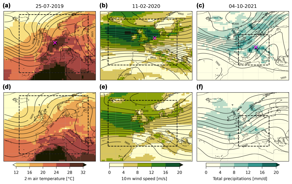
Figure 1 Synoptic situation and observables considered for the three events studied and the composite of their analogues. (a) Geopotential height at 500 hPa (m, contours) and 2 m air temperature (°C, colors) for 25 July 2019, (b) geopotential height at 500 hPa (m, contours) and 10 m wind speed (m s⁻¹, colors) for 11 February 2020, and (c) geopotential height at 500 hPa (m, contours) and total precipitation averaged over 5 d (mm d⁻¹, colors) for 4 October 2021. For all events the dashed black box shows the region where the analogues are computed and the magenta cross shows the grid point taken as the example in Fig. 3. (d–f) The same for the composite of their n=72 analogues.

Here we use the conditional flow analogue attribution methodology proposed by Faranda et al. (2022) and adapted from Yiou et al. (2017). This method is used, for example, by the ClimaMeter tool developed to provide rapid attribution results (Faranda et al., 2024). We propose a procedure to compute both conditional intensity changes and probability ratios when using analogues of the synoptic circulation. We illustrate the procedure on three recent impactful events in Europe: the 25 July 2019 heatwave event in northwestern Europe, the 11 February 2020 wind event in Ireland and the UK, and the 4 October 2021 precipitation event in the Italian Alps. The synoptic situations and the observables considered for the three events are presented in Fig. 1a–c. The 25 July 2019 event was characterized by a strongly meridional meander of the mid-level jet which led to exceptional heat in northern France, Belgium, western Germany and southern England (Fig. 1a; see also Vautard et al., 2020). The 11 February 2020 event coincided with the presence of Storm Ciara in western Europe and led to important wind damage in Ireland, the UK, France, Belgium and the Netherlands (Fig. 1b; Galvin, 2022). Finally, the 4 October 2021 event was an extreme Mediterranean episode which led to intense precipitation in northern Italy and southeast France (Fig. 1c; Cassola et al., 2023).

The paper is organized as follows. In Sect. 2 we present the data used and the method employed. We especially detail the hypotheses of the method and the statistical procedure employed to test the significance of the results obtained. The results are presented in Sect. 3. We discuss these results and the limits of the method in Sect. 4. Finally, the conclusions are drawn in Sect. 5.

2 Data and method

2.1 Data

For all the analyses presented here we use the ERA5 reanalysis data set over the period 1950–2021 (Hersbach et al., 2020). We consider daily mean fields for the geopotential height at 500 hPa (z₅₀₀, 2 m air temperature (t2m​​​​​​​) and 10 m wind speed (wind₁₀), and we use a 5 d rolling mean for total daily precipitation (tp). Using a 5 d rolling mean for precipitation allows us to focus on the synoptic driving rather than on the day-to-day variability in this variable. Note that the ERA5 reanalysis procedure does not assimilate precipitation data and can present important biases with respect to observational data sets (Lavers et al., 2022; Xu et al., 2022). The absolute values provided here must therefore be taken with care. We nevertheless choose to use ERA5 precipitation data for consistency with the other fields and because this paper proposes a methodological development rather than a formal attribution study. We regrid the original 0.25° ERA5 resolution to a 1° resolution for the fields studied here. The reason for using such a lower resolution is that, with the analogue method and using a limited-size data set, the analogues found can be slightly shifted horizontally. This would also correspond to a horizontal shift of the observables of interest, and therefore we cannot expect to reconstruct properly their distributions at the original 0.25° resolution.

For estimating trends, we regress quantities of interest on the regional mean surface temperature (RMST) rather than on the global mean surface temperature (GMST). We make this choice to encompass the local warming trend which can result from additional mechanisms compared to the GMST, for example aerosols concentrations and land-cover changes (Robin and Ribes, 2020; Schumacher et al., 2024). RMST is computed as the area-weighted average of t2m between 35–70° N and 15° W–30° E over both land and ocean, and we then twice apply an 11-year rolling mean as a low-pass filter to obtain a smoothed time series. We note that this simple procedure tends to underestimate the actual warming of Europe for the last years of the time series because there are no data for the years after 2023 in our data set to compute the rolling mean. This would therefore make our results conservative when drawing conclusions on the anthropogenic influence on the events studied.

2.2 Analogue attribution: computation of intensity change and probability ratio

The flow analogue attribution methodology is based on the idea of finding synoptic circulation patterns – called analogues – in the past that are similar to the pattern observed for the extreme event and comparing the hazards they produce. Here we look for analogues of the synoptic circulation using geopotential height at 500 hPa (z₅₀₀) for the three events as it acts as an approximate streamfunction of the free-troposphere atmospheric circulation. There is a positive trend in the geopotential height field which reflects the thickening due to warming of the atmosphere and can lead to finding inappropriate analogues. To avoid this effect, we uniformly detrend the geopotential height field against RMST. We emphasize that doing so only shifts the z₅₀₀ patterns vertically while keeping the correct latitudinal and longitudinal gradients from which the winds can be derived using the geostrophic approximation.

The analogues are found over the period 1950–2021 – without separation into two periods as in Faranda et al. (2022) – using the domains shown in Fig. 1 (dashed boxes): 30–68° N and 20° W–25° E for the temperature event, 35–65° N and 25° W–20° E for the wind event, and 35–55° N and −3° W–17° E for the precipitation event. These domains are chosen using our own expert judgment to find the synoptic structures associated with the events considered, as is customary in attribution studies. We explore the sensitivity of the results obtained in the following by shrinking and expanding these domains by 3° of latitude and longitude at each edge. For our analysis, we take the 72 best analogues as the synoptic patterns minimizing the pointwise Euclidean distance with respect to the synoptic pattern of the event. This is equivalent to finding approximately one analogue per year, although we emphasize that we do not impose the condition that one analogue per year has to be found (there can be several analogues per year). We only impose the condition that the analogues should be separated by at least 5 d, and we exclude the event itself as an analogue. In order to take into account the seasonal cycle and to be close to the observed event, we impose the condition that the analogues must be found in certain months: June to August for the temperature event, October to March for the wind event and September to November for the precipitation event. We also test the sensitivity of the results to the number of analogues found by increasing and decreasing the number of analogues by 25 % (54 and 90 analogues).

To check the quality of the analogues found with our procedure, as in Faranda et al. (2022), we compute the analogue quality metric Q. For each event, its quality Q is computed as the average Euclidean distance of its n=72 analogues. For each analogue k of each event, its own analogue quality metric Q^k is then computed as the average Euclidean distance from its n=72 closest analogues computed over the same domain and time period as for the event. These need not a priori be the same as the n=72 analogues of the event itself. In other words, the fact that a pattern A is among the n=72 closest analogues of a pattern B does not necessarily mean that pattern B is among the n=72 closest analogues of pattern A. We then compare the value of the analogue quality Q^event for the event with the distribution of the ${\left(Q^k\right)}_{\mathrm{1}\le k\le n}$ of its analogues. If Q^event is a clear outlier of the distribution of ${\left(Q^k\right)}_{\mathrm{1}\le k\le n}$ – for example if it is higher than the maximum of ${\left(Q^k\right)}_{\mathrm{1}\le k\le n}$ – this means that the synoptic pattern of the event is unique and therefore that it has bad analogues. In this case, a conditional (and probably also unconditional) attribution statement is likely impossible based on past data only.

As a result of this procedure, we have n=72 analogue dates for each event and therefore n observables of interest (temperature, wind, precipitation) ${\left(X_{i,j}^k\right)}_{\mathrm{1}\le k\le n}$ at each grid point i,j. For these n dates, we also have n values of RMST: ${\left({\mathrm{RMST}}^k\right)}_{\mathrm{1}\le k\le n}$. As in the EVT-based approach, the results obtained will crucially depend on the hypothesis made to relate the ${\left(X_{i,j}^k\right)}_{\mathrm{1}\le k\le n}$ and the ${\left({\mathrm{RMST}}^k\right)}_{\mathrm{1}\le k\le n}$. Here, we follow the practice of current attribution methods (Philip et al., 2020) and assume a linear link for temperature and wind,

$$\begin{array}{}\text{(1)}& X_{i,j}^k={\mathit{\alpha }}_{i,j}+{\mathit{\beta }}_{i,j}{\mathrm{RMST}}^k+{\mathit{ϵ}}_{i,j},\end{array}$$

and a log-linear link for precipitation,

$$\begin{array}{}\text{(2)}& \ln X_{i,j}^k={\mathit{\alpha }}_{i,j}+{\mathit{\beta }}_{i,j}{\mathrm{RMST}}^k+{\mathit{ϵ}}_{i,j},\end{array}$$

the latter expressing a Clausius–Clapeyron-like relationship between global/regional temperatures and precipitation. The ϵ_i,j terms are random terms with a hypothesized parametric distribution (see below). The α_i,j and β_i,j are then determined by ordinary least-squares (OLS) regression. The intensity change IC_i,j at grid point i,j is therefore computed as

$$\begin{array}{}\text{(3)}& {\mathrm{IC}}_{i,j}={\mathit{\beta }}_{i,j}\times ({\mathrm{RMST}}_{\mathrm{event}}-{\mathrm{RMST}}_{\mathrm{1950}})\end{array}$$

for temperature and wind and as

$$\begin{array}{}\text{(4)}& {\mathrm{IC}}_{i,j}=X_{i,j}^{\mathrm{event}}-X_{i,j}^{\mathrm{event}}{e}^{{\mathit{\beta }}_{i,j}({\mathrm{RMST}}_{\mathrm{1950}}-{\mathrm{RMST}}_{\mathrm{event}})}\end{array}$$

for precipitation. Here RMST_event is the RMST for the event (assumed to be the factual world) and RMST₁₉₅₀ is the RMST in 1950 (assumed to be the counterfactual world). For precipitation, $X_{i,j}^{\mathrm{event}}$ is the intensity of the event at grid point i,j.

At this stage, we detrend the time series ${\left(X_{i,j}^k\right)}_{\mathrm{1}\le k\le n}$ with the coefficients determined above to obtain a new time series ${\left({\stackrel{\mathrm{̃}}{X}}_{i,j}^k\right)}_{\mathrm{1}\le k\le n}$. This time series is an empirical sampling (up to the detrending procedure) of the distribution ${\stackrel{\mathrm{̃}}{X}}_{i,j}|\mathcal{C}$ of the observable ${\stackrel{\mathrm{̃}}{X}}_{i,j}$ conditional on the synoptic situation 𝒞 of the extreme event. If we had enough data – i.e., a longer-running data set and therefore more analogues – we could give an empirical estimation of the probability of reaching level ${\stackrel{\mathrm{̃}}{X}}^{\mathrm{event}}$ for this conditional distribution. Considering that ${\stackrel{\mathrm{̃}}{X}}^{\mathrm{event}}$ is likely extreme – even when conditioning on the synoptic pattern 𝒞 – it is usually not possible to give a precise empirical value to this probability. We therefore need to use a parametric hypothesis to estimate probabilities in both worlds. The difficulty is that, contrary to the EVT-based method, we have no a priori choice for what distribution ${\stackrel{\mathrm{̃}}{X}}_{i,j}|\mathcal{C}$ should follow. Here, we propose to use the skew-normal distribution for temperature and wind and the gamma distribution for precipitation (see Sects. 3 and 4 for a discussion on the choice of these probability distributions). We fit a skew-normal or gamma distribution to the ${\left({\stackrel{\mathrm{̃}}{X}}_{i,j}^k\right)}_{\mathrm{1}\le k\le n}$ using the method of moments. The choice of this method for the fits was made to speed up computations considering the large number of fits necessary with our bootstrap procedure (see below and Appendix A for the detail of the method of moments for the skew-normal and gamma distributions). Once we have access to the parameters of the distribution, we evaluate the probability of $X_{i,j}^{\mathrm{event}}$ for these distributions in the counterfactual world and in the factual world. For the skew-normal distribution, this procedure means shifting the fitted location parameter by β_i,jRMST₁₉₅₀ (counterfactual world) and β_i,jRMST_event (factual world). For the gamma distribution, this is equivalent to multiplying the scale parameter by $e^{{\mathit{\beta }}_{i,j}{\mathrm{RMST}}_{\mathrm{1950}}}$ (counterfactual world) and $e^{{\mathit{\beta }}_{i,j}{\mathrm{RMST}}_{\mathrm{event}}}$ (factual world).

The full procedure can be summarized as follows:

1. Find n analogues over the period 1950–2021.

2. Extract the n values of the observable X at grid point i,j: ${\left(X_{i,j}^k\right)}_{\mathrm{1}\le k\le n}$.

3. Extract the n values of RMST: ${\left({\mathrm{RMST}}^k\right)}_{\mathrm{1}\le k\le n}$.

4. Detrend the time series ${\left(X_{i,j}^k\right)}_{\mathrm{1}\le k\le n}$ with respect to ${\left({\mathrm{RMST}}^k\right)}_{\mathrm{1}\le k\le n}$, linearly for temperature and wind and log-linearly for precipitation.

5. Compute the intensity change as the difference between the event and the projection of the event in 1950 based on the detrending hypothesis.

6. Fit a parametric distribution to the detrended time series ${\left({\stackrel{\mathrm{̃}}{X}}_{i,j}^k\right)}_{\mathrm{1}\le k\le n}$, a skew-normal distribution for temperature and wind and a gamma distribution for precipitation.

7. Compute the probabilities for the present event and 1950 using the fitted distribution and evaluate the probability ratio $\mathbb{P}(X\ge x|F=\mathrm{1})/\mathbb{P}(X\ge x|F=\mathrm{0})$.

We assess the sensitivity of the results obtained using a bootstrap procedure: at each grid point i,j we resample 10³×n values of the analogue observables ${\left(X_{i,j}^k\right)}_{\mathrm{1}\le k\le n}$ with replacement and execute the procedure described above. We report the median value of the 10³ resamplings. This result is said to be significant if the critical value (0 for the intensity change and 1 for the probability ratio) is either above the 97.5th quantile or below the 2.5th quantile of the 10³ resamplings. The same procedure is applied to each grid point i,j, all grid points being treated independently.

2.3 EVT-based attribution

We additionally compare our procedure to the unconditional EVT approach. To do so, at each grid point i,j we compute the yearly maxima of the observable of interest, restricting the time span to the same months as the ones over which the analogues are computed (June to August for the temperature event, October to March for the wind event, September to November for the precipitation event). We then detrend this time series of yearly maxima and compute the intensity change similarly to the method presented above for the analogue procedure. We emphasize however that there is no a priori reason that the intensity change computed on the yearly maxima should be similar to the one for the analogue distribution because the yearly maxima may not correspond to analogues of the event. We then fit a GEV distribution to the detrended time series using the method of L-moments (Hosking, 1990). The probabilities in the counterfactual and factual worlds are recovered as above by shifting the location parameter by β_i,jRMST₁₉₅₀ and β_i,jRMST_event for temperature and wind and multiplying the location and scale parameters by $e^{{\mathit{\beta }}_{i,j}{\mathrm{RMST}}_{\mathrm{1950}}}$ and $e^{{\mathit{\beta }}_{i,j}{\mathrm{RMST}}_{\mathrm{event}}}$ for precipitation. From these probabilities we recover the probability ratio. To estimate the sensitivity of these results, we also use a bootstrap procedure with 10³ resamplings, and we report the median result when it is significant.

We note that this procedure is not exactly the same as the one of the World Weather Attribution (Philip et al., 2020), which directly fits a non-stationary GEV with the maximum likelihood method. We made this choice here in order to be more similar to our procedure for the analogue-based attribution. Nonetheless, this procedure can be adapted straightforwardly if one wants to use the maximum likelihood method with non-stationary skew-normal, gamma and GEV distributions.

3 Results

3.1 Illustration of the method with three grid points

To investigate the relevance of the analogues found for the three events, in Fig. 1d–f we show the composite fields of z₅₀₀ and of the observables of interest (temperature, wind and precipitation). The n=72 analogues found for each event are shown in Figs. B1, B2 and B3. For the temperature and wind events, the synoptic situation is qualitatively similar to the event itself, and so are the observable fields, although with an intensity that is less than that of the events as can be expected because we are investigating extreme situations. For the temperature event, the mid-tropospheric flow is nonetheless less meridional than for the event. The synoptic situation for the precipitation events is not as satisfying insofar as the composite does not show the secondary trough that can be seen over the eastern Pyrenees in Fig. 1c and the downstream ridge is less intense than for the event. Despite this discrepancy, the structure of the precipitation field is qualitatively similar to the one of the event itself, with precipitation in southeast France and northern Italy.

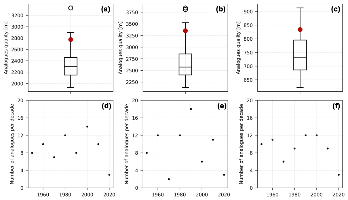
Figure 2 Analogue quality and trend in the number of analogues per decade. First row: distribution of the analogue quality over the 72 analogues for (a) the 25 July 2019 event, (b) the 11 February 2020 event and (c) the 4 October 2021 event. The boxplots show the 25th and 75th quantiles and the median of the distribution. For each plot, the red dot shows the analogue quality for the event itself. Second row: number of analogues per decade for (d) the 25 July 2019 event, (e) the 11 February 2020 event and (f) the 4 October 2021 event.

In Fig. 2a–c, we show the distributions of Q^k for the analogues found (boxplots) and the analogue quality Q for the event itself (red dot). The analogue quality metrics Q of all events are in the upper tail of the distribution of Q^k – which may be expected insofar as they are all rare events – but are not outliers of the distributions. There are 4 analogues with worse analogue quality for the temperature event, 3 for the wind event and 8 for the precipitation event. Figure 2d–f show the number of analogues per decade for each event. We compute the linear trend over this number of analogues to explore whether they have become more likely with time. The significance of the trend is computed using a bootstrap procedure: we resample 10³×72 analogues and compute the trend. If the value 0 is outside the 95 % interval centered around the median of these trends, then the trend is said to be significant. Note that because we have only 2 years in the 2020 decade, these years are not taken into account for computing the trend. For none of the events is this trend significant, which shows that the analogues are well distributed over the period 1950–2021.

In order to give probability ratios measuring the increasing/decreasing likelihood of the extreme events considered, we need to rely on a parametric hypothesis for the distribution of the observable conditional on the synoptic pattern of the event. If we had a much larger sample size than the one ERA5 reanalysis provides, we could compute empirical probabilities, and this could for example be done with either a long run or a large ensemble of a climate model. Contrary to the EVT approach to attribution, which is based on a theoretical result that provides which parametric distributions should be used for computing probability ratios, here we have no a priori theoretical basis for which distribution to use. Figure B4 shows the empirical skewness (first row) and excess kurtosis (second row) for the analogue distributions of the observables for the three events considered (after the detrending procedure). We assess the statistical significance of these quantities using the same bootstrap procedure as the one described for the analogue attribution (see Sect. 2) and show in white grid points those which are not statistically significant. These results should nevertheless be taken with care as the precise estimation of the third and fourth moment with n=72 is difficult. For temperature and wind (Fig. B4a, b, d and e), most of the grid points do not show a significant departure from 0, i.e., from the third and fourth moments of a Gaussian distribution. Temperature tends to be negatively skewed over sea surfaces (Fig. B4a), and wind tends to be negatively skewed over sea surfaces in northern Europe and positively skewed over the Mediterranean land surfaces (Fig. B4b), but for both observables, the departure from 0 is small over the regions of interest for both events, except over the North Sea for the wind event. Similarly, the excess kurtosis is not different from 0, and, if anything, it tends to be slightly negative – although this may arise as the result of under-sampling the very extremes. As a consequence, we propose to use the skew-normal distribution – which is a modification of the Gaussian distribution to take into account the skewness of the distribution (see Appendix A) – to represent the analogue distribution of these observables at each grid point.

For precipitation (Fig. B4c and f) the results are different. The conditional distribution is significantly positively skewed for most grid points, as expected for an observable which is bounded downwards by 0, and the excess kurtosis is not significantly different from 0 for most land grid points. For grid points where the excess kurtosis is significant, it is strongly positive, which would be likely to be the same for most grid points if we had more analogues insofar as precipitation distributions are usually long tailed. As a consequence, we treat the precipitation observable differently and use a gamma distribution to fit its distribution. The gamma distribution is commonly used to fit precipitation data (Stagge et al., 2015; Gudmundsson and Seneviratne, 2016; Martinez-Villalobos and Neelin, 2019). We come back to the question of the choice of these distributions in the Discussion section.

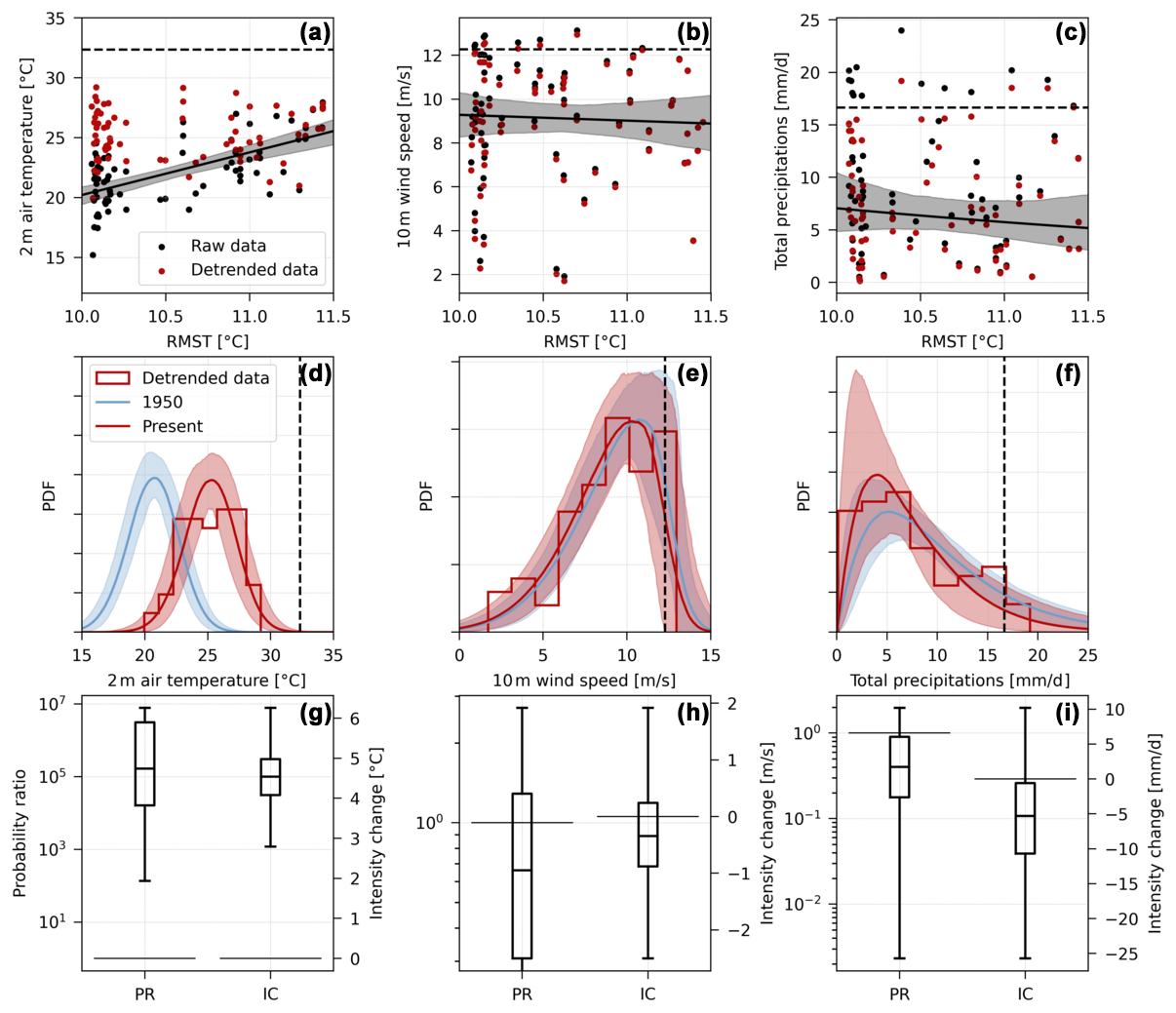
Figure 3 Illustration of the analogue attribution method for the three example grid points of Fig. 1. First row (a–c): raw values of the analogue observables (black dots) and detrended values of the analogue observables (red dots) vs. RMST. The detrended values are shifted to the 2020 RMST value. The observables are detrended to correspond to the RMST of the event. The solid black line and the black shading show the median regression line and the 95 % uncertainties interval for the regression of the raw values of the analogue observables against RMST. The horizontal dashed black line shows the intensity of the event. Note that for panel (c) the regression is logarithmic with respect to RMST (see Sect. 2). Second row: fitted (d, e) skew-normal and (f) gamma distributions for RMST in 1950 and in the present (i.e., for the event). The solid line shows the median fit and the shading the 95 % uncertainty interval obtained after bootstrapping (see Sect. 2). The empirical histogram corresponds to the detrended values of the analogue observables. The vertical dashed black line shows the intensity of the event. Third row (g–i): bootstrap distribution of probability ratios and intensity changes for the events. For the probability ratios, the horizontal black line shows the value 1 (no probability change). For the intensity changes, the horizontal black line shows the value 0 (no intensity change).

Figure 3 shows an illustration of our method on three example grid points marked by a magenta cross in Fig. 1. For the 25 July 2019 temperature event, the intensity reached is so extreme that it is never reached by its analogues, even after detrending the analogue observables of the past (Fig. 3a). As a consequence, it is in the far tail of the fitted distributions for both the past (1950) and the present (2019, Fig. 3d) and the probability ratios are largely higher than 1, with a median value around 10⁵. Accordingly, the median intensity change is around 4.5 °C. For the 11 February 2020 wind event, the event itself was intense but four analogues in the past show higher values than the event. The trend of the analogue observables with respect to RMST is weak, and as a consequence, the conditional distributions in the past and the present are close. The median probability ratio is around 0.7 and the median intensity change around −0.5 m s⁻¹, but none of these values are statistically significant according to the bootstrap procedure. For the 4 October 2021 precipitation event, the event itself was also intense but exceeded by 13 analogues in the past. The logarithmic regression points towards a small decrease in the intensity of these events, which slightly decreases the intensity of the analogue events as projected in 2021 (Fig. 3c). The event therefore becomes slightly more unlikely in the present (Fig. 3f), and the median probability ratio is around 0.7 with an intensity change of around −5 mm d⁻¹, but these changes are not statistically significant. To test the parametric hypothesis made for computing the probability ratios, we employ the two-sided Kolmogorov–Smirnov test on each resampled time series to test the hypothesis that the distribution of the resampled time series is different from the fitted distribution, i.e., a skew-normal distribution for temperature and wind and a gamma distribution for precipitation. Using the 5 % confidence level, 99.9 % of the resampled time series are not distinguishable from the target distribution for the temperature and wind events and around 99 % are not for the precipitation event. This shows that the chosen distributions are compatible with the data.

3.2 Results in Europe

We apply the same procedure to every grid point in Europe. The results for the median probability ratios and intensity changes are shown in Fig. 4. For the intensity changes, in addition to the observable considered, we also show the significant changes in the synoptic field (geopotential height at 500 hPa). The temperature event is associated with significant increases in probability ratios over western Europe, especially in northern France, Belgium, the Netherlands and southern England, where they are higher than 10³ (Fig. 4a). The intensity changes show a similar pattern (Fig. 4d), although with interesting differences: whereas the intensity changes are similar in northeast Spain to the ones in northern France, Belgium and southern England, the probability ratios of the former are smaller. This likely reflects different scales and shapes of the fitted distributions of the observables. The wind event presents no changes in the probability ratios. In the main zone of interest for the event (Ireland, the UK and the North Sea), no grid points show a significant change (Fig. 4b), which is also reflected in the intensity changes (Fig. 4e). For the precipitation event, except for some grid points in southeast France, most grid points do not show significant values in the probability ratio and the intensity change (Fig. 4c). Finally, we note that the changes in the synoptic fields for all events are minimal or nonexistent: there is a small increase in the intensity of the anticyclone over the ocean west of Brittany for the temperature event and no changes for the wind and precipitation events. Figure B5 in the Appendix shows at each grid point the proportion of resampled time series which pass the Kolmogorov–Smirnov test at the 5 % level, i.e., the proportion of the resampled time series for which the proposed distribution is a correct representation of the empirical distribution. For all events, over the regions of interest this proportion is higher than 90 % and close to 100 % for most grid points.

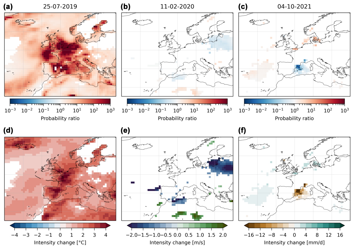
Figure 4 Probability ratios and intensity changes with the analogue method. First row (a–c): median probability ratios obtained at each grid point for (a) the temperature event, (b) the wind event and (c) the precipitation event. The grid points are colored in white when the probability ratios are not statistically different than 1 (see Sect. 2). Second row (d–f): median intensity changes for the observable (colors) and the synoptic field (z₅₀₀ in m, contours). For the observable, the grid points are colored in white when the intensity change is not statistically different than 0 (see Sect. 2). For the synoptic field, the intensity change is not shown when it is not statistically different than 0.

To test the sensitivity of these results, we present similar figures to Fig. 4 in the Appendix, where we change the number of analogues by ±25 % (54 and 90 analogues over 1950–2021, Figs. B6 and B7) and the size of the domain to find analogues within ±3° of longitude and latitude at the edge of the domains defined in Fig. 1 (Figs. B8 and B9). For the temperature event, the results presented above are stable regardless of a change in the number of analogues and in the size of the domain. This likely reflects the strong warming in extreme temperatures observed in western Europe and already discussed by several previous works (Vautard et al., 2023; Patterson, 2023; Noyelle et al., 2023). For the wind event, the results obtained tend to be similar, with no detectable changes. Finally, for the precipitation event in southeast France and the Italian Alps, the changes are mostly insignificant even though some grid points see a significant decrease between 5 and 10 mm d⁻¹.

3.3 Comparison with the climatological and EVT-based approaches

The intensity changes presented in Fig. 4 are computed conditionally on the analogues, i.e., on the synoptic pattern of the extreme events observed. To investigate the difference with respect to conditioning on the analogues compared to other methods, in Fig. 5a–c we present the intensity changes deduced from the climatological trends computed on the months when the analogues are found. At each grid point, we compute the intensity change as previously, but this time the trend is computed by considering all days of the months when the analogues are searched (June to August for the temperature event, October to March for the wind event, September to November for the precipitation event). Figure 5d–f show the difference with the analogue intensity changes when they are statistically significant according to the bootstrap procedure, as previously. For the temperature and precipitation events, the intensity changes conditional on the analogues over the regions of interest for the extremes are stronger than the climatological trends, and they are even the reverse for the precipitation events. This demonstrates the contribution of conditioning on the analogues. For the wind events there are weak or no trends in the region of interest for both the climatology and the analogues. We could in principle do the same analysis for probability ratios, but we would need to make a parametric assumption about the full distribution of the observable over the months considered, which is likely more difficult than for the distribution conditional on the analogues.

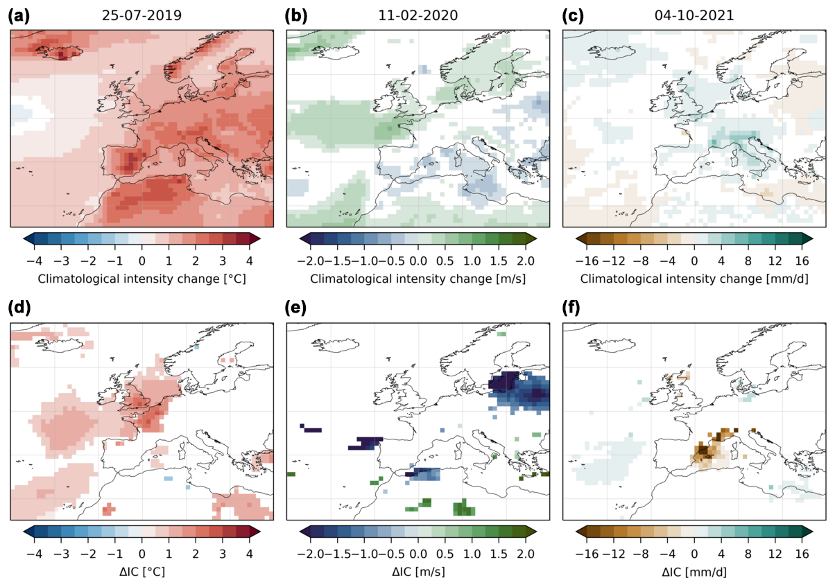
Figure 5 Climatological intensity changes and comparison with analogue intensity changes. First row (a–c): median climatological intensity changes based on the trend over the months where the analogues are searched for. Second row (d–f): difference between climatological intensity changes and analogue intensity changes of Fig. 4. The grid points are colored in white when the difference is not statistically significant according to the bootstrap procedure (see Sect. 2).

Finally, we compare our results with the classical EVT-based approach for extreme events. The EVT approach is unconditional and compares the intensity of the event observed to a non-stationary GEV distribution fitted to the yearly maxima over the period 1950–2021. Figure 6 shows the results with this approach for the three grid points studied in Fig. 3. For the temperature event, both approaches conclude that there is an increasing probability and intensity of this event but the EVT approach provides lower probability ratios and intensity changes (Fig. 3g vs. Fig. 6g). For the wind event, both approaches give similar non-significant results for the grid point selected (Fig. 3h vs. Fig. 6h). Lastly, for the precipitation event, the EVT approach gives a non-significant result but points towards an increase in the probability and intensity of this event, which is contrary to the analogue approach (Fig. 3i vs. Fig. 6i).

Figure 6 The same as Fig. 3 with the EVT approach.

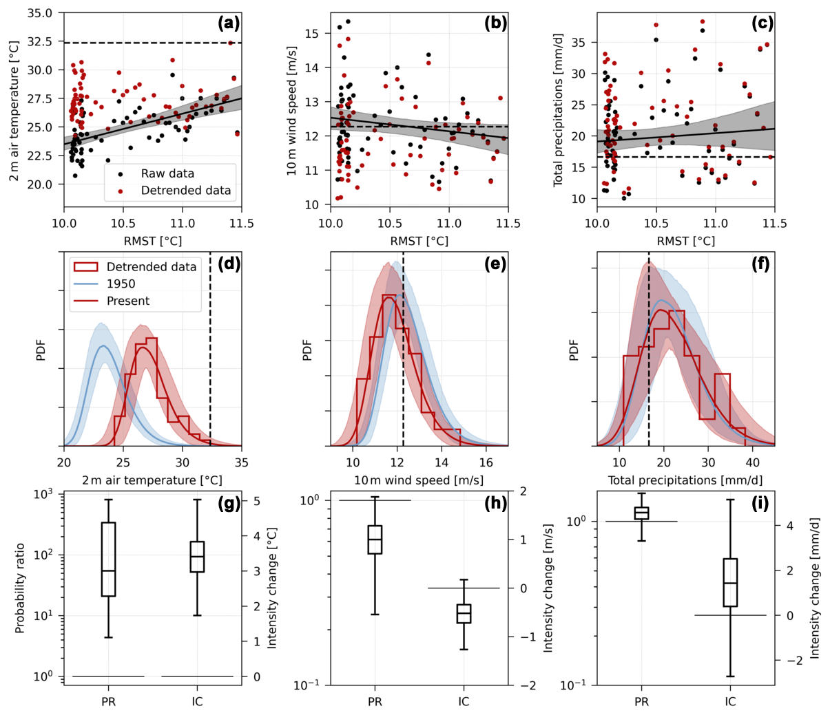
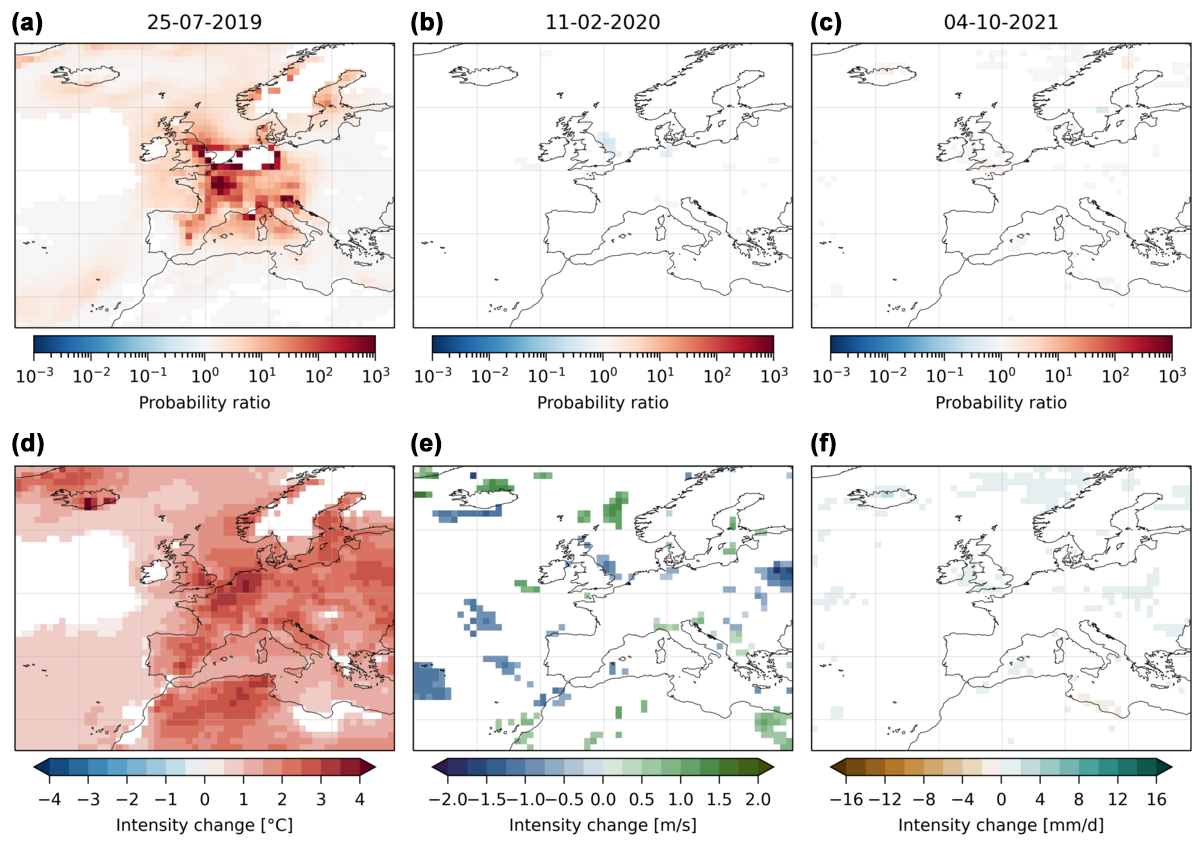
Figure 7 The same as Fig. 4 with the EVT approach.

Figure 7 shows the equivalent of Fig. 4 with the EVT approach. It displays the median probability ratios and intensity changes found with the EVT approach after 10³ resamplings when they are statistically significant at each grid point. The results obtained are rather different from the analogue approach. For the temperature event, the significant probability ratios tend to be confined to western Europe (especially France) and the intensity changes are smaller than the ones observed with the analogue method. For the wind event, only few and sparse grid points show a significant change. The precipitation event also does not show significant changes over most of Europe and especially in the Italian Alps. This result is mostly similar to the one obtained with the analogue method, despite some grid points showing a significant decrease, especially in southeast France. We come back to this discrepancy in the Discussion section. Note that for precipitation, it is not clear that yearly maxima have converged towards a GEV distribution and it may be more suitable to use larger block sizes (Alaya et al., 2020), although this would reduce the sample sizes for the fits.

4 Discussion

In this paper we propose to estimate intensity changes and probability ratios for the flow analogue extreme event attribution method. The main improvement compared to the method proposed by Faranda et al. (2022) is to avoid the arbitrary split of the analogues into two periods. Doing so increases the number of analogues found and therefore gives more statistical strength to the results obtained, even though we have to make some additional statistical assumptions.

Our procedure estimates intensity changes by regressing the observables of interest on a metric measuring anthropogenic global warming – regional mean surface temperature (RMST) here. We applied this method grid point by grid point, but it could be applied, for example, over a spatial average to study a particular region of interest. The hypotheses made to estimate intensity changes are minimal and unrelated to the parametric assumption for the computation of the probability ratios. The results obtained can thus be considered a good approximation of the response to increasing RMST of the mean of the observables of interest conditional on the synoptic pattern of the event of interest (as soon as they are stable with respect to small changes in the number of analogues and the domain to compute analogues). The intensity changes thus give an estimate of the mean observed thermodynamical response for a particular synoptic-scale pattern.

The hypotheses made to estimate probability ratios on the other hand are more problematic because they rely on a parametric approximation. If the fitted distributions for the conditional distribution of the observable are incorrect, this could lead to large errors in the estimated probability ratios, especially when the extreme event studied is largely outside the distribution of its analogues (such as for the 25 July 2019 temperature event). Here we presented arguments based on the third and fourth moments of the conditional distributions to justify the use of skew-normal distributions for temperature and wind and gamma distributions for precipitation. We nevertheless acknowledge that these arguments are based on empirical results and have to be tested case by case. As a consequence, it is likely that the choice of the fitted distributions can be questioned and could be adapted to find more suitable distributions for the estimation of probability ratios for other events and other observables. Moreover, even with our parametric choice, as illustrated here in Figs. 3 and 6, the range of uncertainties in the probability ratios can be several orders of magnitude large according to the bootstrap procedure. This is a known problem for risk-based extreme event attribution method which arises as a result of the estimation of a ratio of low or very low probabilities. It is however not even clear that the mean value of this ratio is well defined statistically – for example if the mean probability of the event in the counterfactual world is equal to 0. For these reasons, it is probably more meaningful to be cautious and use intensity changes rather than probability ratios for reporting attribution results. As a consequence, the parametric hypotheses made to represent the probabilities conditional on the synoptic pattern may not be that important to establishing an attribution statement for extreme events, as soon as the intensity change is significantly different from 0.

Similarly to the EVT-based attribution method, the flow analogue method may suffer from an under-sampling of extremes due to the use of a limited-size reanalysis data set only. In other words, good analogues need to be found for the conditional attribution to make sense, and therefore the strongest unprecedented extreme events may not be attributable with this method if they have no past analogues. This method can straightforwardly be used with climate models outputs to strengthen the analysis, especially with large ensembles to find more analogues. Conditioning on a measure of global warming as done here could also allow the comparison of results for models with different climate sensitivities. However, models have known deficiencies, including biases (Maraun, 2016; Vrac et al., 2023; François et al., 2020) and incorrect dynamics of extremes under forcing over western Europe (Van Oldenborgh et al., 2022; Patterson, 2023; Vautard et al., 2023; D'Andrea et al., 2024), which may not counterbalance the sampling issue of the reanalysis. Another sampling issue concerns the natural variability in the climate system. If a long-term physical phenomenon has covaried over a long period of time with RMST and can influence the intensity of the events studied, then this would lead to an incorrect estimation of the impact of global warming per se. Using analogues over 72 years, as done here, partially alleviates this risk compared to separating them into two periods as in Faranda et al. (2022), especially when they are well distributed over time with little increasing or decreasing trend (Fig. 2). Another way to circumvent this issue could be to include measures of natural variability on the regressions of the observable, for example the Atlantic Meridional Variability (AMV) for extremes in Europe (Suarez-Gutierrez et al., 2023).

We nevertheless want to note that the main drawbacks of the method presented here are also common to the classical EVT method, namely under-sampling, representation of natural variability, and use of past observations vs. model outputs. The interpretation of the results is also different between the two approaches. The EVT-based approach gives the probability that the yearly maximum of an observable is above a given level, and therefore the probability ratio indicates how this probability has changed between the factual and counterfactual worlds. It thus encompasses both the dynamical changes – increasing frequency of certain weather patterns caused by anthropogenic global warming (Vautard et al., 2023; Faranda et al., 2023; Dong et al., 2024; D'Andrea et al., 2024) – and the thermodynamical changes for the strongest extremes. As a consequence, its analysis may be far from the actual extreme event observed and in particular can always make an attribution statement even though the dynamics of the event has never been observed in the past at the place considered (Faranda et al., 2024). The flow analogue method on the other hand gives the change in the probability of a certain level given the synoptic pattern as soon as the synoptic pattern has good analogues in the past. This method separates the dynamical contribution from the thermodynamical contribution. It does not address the unconditional probability of reaching an extreme – which may be the most interesting aspect for the general public – but it tends to give a better attribution signal because thermodynamical changes are likely more easily detectable than dynamical changes (Shepherd, 2014; Vautard et al., 2023). Our results suggest that the EVT-based approach may tend to be too conservative in its attribution statements by considering only the strongest extremes for which rare or very rare dynamical mechanisms may overrun the climate change thermodynamical signal.

As illustrated, the two methods do not give the same absolute results in general and may also give opposing results, as is suggested for the precipitation event here. For this event in particular, contrary to the previous literature (Min et al., 2011; Fischer and Knutti, 2015; Donat et al., 2016; Pfahl et al., 2017; Tramblay and Somot, 2018; Zittis et al., 2021), we tend to see no change or a small decrease in the intensity of precipitation conditional on the analogues. This result is surprising and goes against the Clausius–Clapeyron scaling for the strongest precipitation events. However, when looking at the trend in the 2 m air temperature for the analogues of this event, we found no significant trend in the region investigated (not shown), which does not come from a change in the seasonality of the analogues found over 1950–2021. This may explain why we observe no significant change and may arise from the fact that analogues of this particular synoptic pattern do not show a significant warming response. This however may also be due to the fact that no or few good analogues of this event exist in the reanalysis. The intensity of precipitation events is forced both by synoptic-scale and mesoscale structures: while there may be good analogues of the latter, the former are likely not well sampled in the ERA5 reanalysis. This leads us to advocate for a cautious use of the flow analogue attribution method for intense precipitation events, especially when most precipitation is convective.

When two attribution methods differ in their results, as shown here, it is not clear which one should be preferred. The unconditional attribution method likely gives a more general and useful answer for the general change in the intensity of extremes, which is the most relevant to adaptation purposes. However, conditional attribution methods, such as the one presented here or others (Yiou et al., 2017; Terray, 2021; de Vries et al., 2024; Leach et al., 2024), are more focused on the very dynamics of the event observed and may provide a more detectable (thermodynamical) signal. The main advantage of our method is to use only past data and therefore to avoid common pitfalls of modeling studies. But, as explained above, the method also has its own issues. As argued recently by Coumou et al. (2024), using a range of methods to provide multiple lines of evidence for an attribution statement useful for practitioners is therefore absolutely necessary.

5 Conclusions

In this paper we proposed a way to compute intensity changes and probability ratios for the flow analogue extreme event methodology proposed by Faranda et al. (2022) and adapted from Yiou et al. (2017). Contrary to Faranda et al. (2022), we do not separate the data sets into two periods but search for analogues of the synoptic pattern of the extreme event in the full data set (1950–2021). We then fit a linear model to the analogue observable of interest to estimate intensity changes with increasing regional mean surface temperature (RMST). We compute probability ratios by making a parametric hypothesis about the distribution of the observables conditional on the synoptic-scale pattern. We finally estimate the sensitivity of the results with a bootstrap procedure and report the median values when they are statistically significant. The method proposed here can be applied to other observables of interest and using outputs of climate models, especially to check the consistency of their thermodynamical evolution for observed weather patterns leading to extremes. One advantage of the method proposed here is that we perform conditioning on a measure of global warming, which, when applied with model outputs, would allow us to compare models with different climate sensitivities. The method nevertheless requires the existence of past good analogues, which may not exist in reanalysis data sets for the most intense and unprecedented extremes.

We illustrate the method using three recent events in Europe: the 25 July 2019 temperature event, the 11 February 2020 wind event and the 4 October 2021 precipitation event. We find that the intensity changes for the temperature event over western Europe are around 4.5°C and the probability ratios above 10³. These results are stable with a change in the parameters of the method, which makes it possible to say that this event was made more likely and more intense under climate change. The intensity changes and probability ratios over Ireland, the UK and the North Sea for the wind event do not detect any change, and this result seems robust to specifications, which suggests that this event was not impacted by AGW. Lastly, the precipitation event in the Italian Alps and southeast France tends to be slightly less likely and intense under climate change, but the results are sensitive to the specification of the method. For the precipitation event, our results with the analogue method tend to be different from the results obtained with the EVT-based method, which suggests a small, insignificant increase in intense precipitation for the region and the period studied. All our attribution statements are conditional on the synoptic-scale pattern observed during the events.

Appendix A: Method of moments for the skew-normal and gamma distributions

A1 Skew-normal distribution

The skew-normal distribution is an adaptation of the Gaussian distribution to account for non-zero skewness. Its probability density function (PDF) can be expressed as

$$\begin{array}{}\text{(A1)}& f\left(x\right)=\mathit{\varphi }\left({\displaystyle \frac{x-\mathit{\mu }}{\mathit{\sigma }}}\right)\mathrm{\Phi }\left(\mathit{\xi }{\displaystyle \frac{x-\mathit{\mu }}{\mathit{\sigma }}}\right),\end{array}$$

where $\mathit{\varphi }\left(x\right)=\frac{\mathrm{1}}{\sqrt{\mathrm{2}\mathit{\pi }}}{e}^{-\frac{\mathrm{1}}{\mathrm{2}}{x}^{\mathrm{2}}}$ is the PDF of the standard normal; $\mathrm{\Phi }\left(x\right)={\int }_{-\mathrm{\infty }}^x\mathit{\varphi }\left(t\right)\mathrm{d}t$ is the cumulative density function (CDF) of the standard normal; and μ, σ and ξ are the location, scale and shape parameters of the distribution.

The method of moments take a simple analytic form for this distribution. Let us note ${\widehat{\mathit{\gamma }}}_{\mathrm{1}}$, the empirical skewness (centered and normalized third-order moment) of the samples $(X^k{)}_{\mathrm{1}\le k\le n}$. We define

$$\begin{array}{}\text{(A2)}& \widehat{\mathit{\delta }}:=\sqrt{{\displaystyle \frac{\mathit{\pi }}{\mathrm{2}}}{\displaystyle \frac{|{\widehat{\mathit{\gamma }}}_{\mathrm{1}}{|}^{\mathrm{2}/\mathrm{3}}}{|{\widehat{\mathit{\gamma }}}_{\mathrm{1}}{|}^{\mathrm{2}/\mathrm{3}}+{\left(\frac{\mathrm{4}-\mathit{\pi }}{\mathrm{2}}\right)}^{\mathrm{2}/\mathrm{3}}}}}.\end{array}$$

From this value, we can derive an estimation of the three parameters of the distribution:

$$\begin{array}{}\text{(A3)}& \left\{\begin{array}{l}\widehat{\mathit{\xi }}=\frac{\widehat{\mathit{\delta }}}{\sqrt{\mathrm{1}-{\widehat{\mathit{\delta }}}^{\mathrm{2}}}}\\ \widehat{\mathit{\sigma }}={\displaystyle \frac{\widehat{s}}{\sqrt{\mathrm{1}-\mathrm{2}{\widehat{\mathit{\delta }}}^{\mathrm{2}}/\mathit{\pi }}}}\\ \widehat{\mathit{\mu }}=\widehat{m}-\widehat{\mathit{\sigma }}\widehat{\mathit{\delta }}\sqrt{{\displaystyle \frac{\mathrm{2}}{\mathit{\pi }}}}\end{array}\right.,\end{array}$$

where $\widehat{m}$ and $\widehat{s}$ are the empirical mean and standard deviation of the samples $(X^k{)}_{\mathrm{1}\le k\le n}$. Note that for the skew-normal distribution, the skewness has a maximum absolute value close to 0.99. Therefore, when applying the method of moments here, we take

$$\begin{array}{}\text{(A4)}& \left|{\widehat{\mathit{\gamma }}}_{\mathrm{1}}\right|=min\left(\mathrm{0.99},\sum _{k=\mathrm{1}}^n{\left({\displaystyle \frac{X^k-\widehat{m}}{\widehat{s}}}\right)}^{\mathrm{3}}\right)\end{array}$$

and $\widehat{\mathit{\delta }}$ has the same sign as ${\widehat{\mathit{\gamma }}}_{\mathrm{1}}$.

A2 Gamma distribution

Here we use the gamma distribution defined on $[\mathrm{0},+\mathrm{\infty })$, i.e., with a null location parameter. The PDF of the distribution is

$$\begin{array}{}\text{(A5)}& f\left(x\right)={\displaystyle \frac{\mathrm{1}}{\mathrm{\Gamma }\left(\mathit{\xi }\right){\mathit{\sigma }}^{\mathit{\xi }}}}{x}^{\mathit{\xi }-\mathrm{1}}{e}^{-x/\mathit{\sigma }},\end{array}$$

where Γ is the gamma function, ξ is the shape parameter and σ is the scale parameter.

The method of moments also takes a simple analytic form for this distribution:

$$\begin{array}{}\text{(A6)}& \left\{\begin{array}{l}\widehat{\mathit{\sigma }}=\frac{{\widehat{s}}^{\mathrm{2}}}{\widehat{m}}\\ \widehat{\mathit{\xi }}=\widehat{m}/\widehat{\mathit{\sigma }}\end{array}\right.,\end{array}$$

where $\widehat{m}$ and $\widehat{s}$ are the empirical mean and standard deviation of the samples $(X^k{)}_{\mathrm{1}\le k\le n}$.

Appendix B: Additional figures

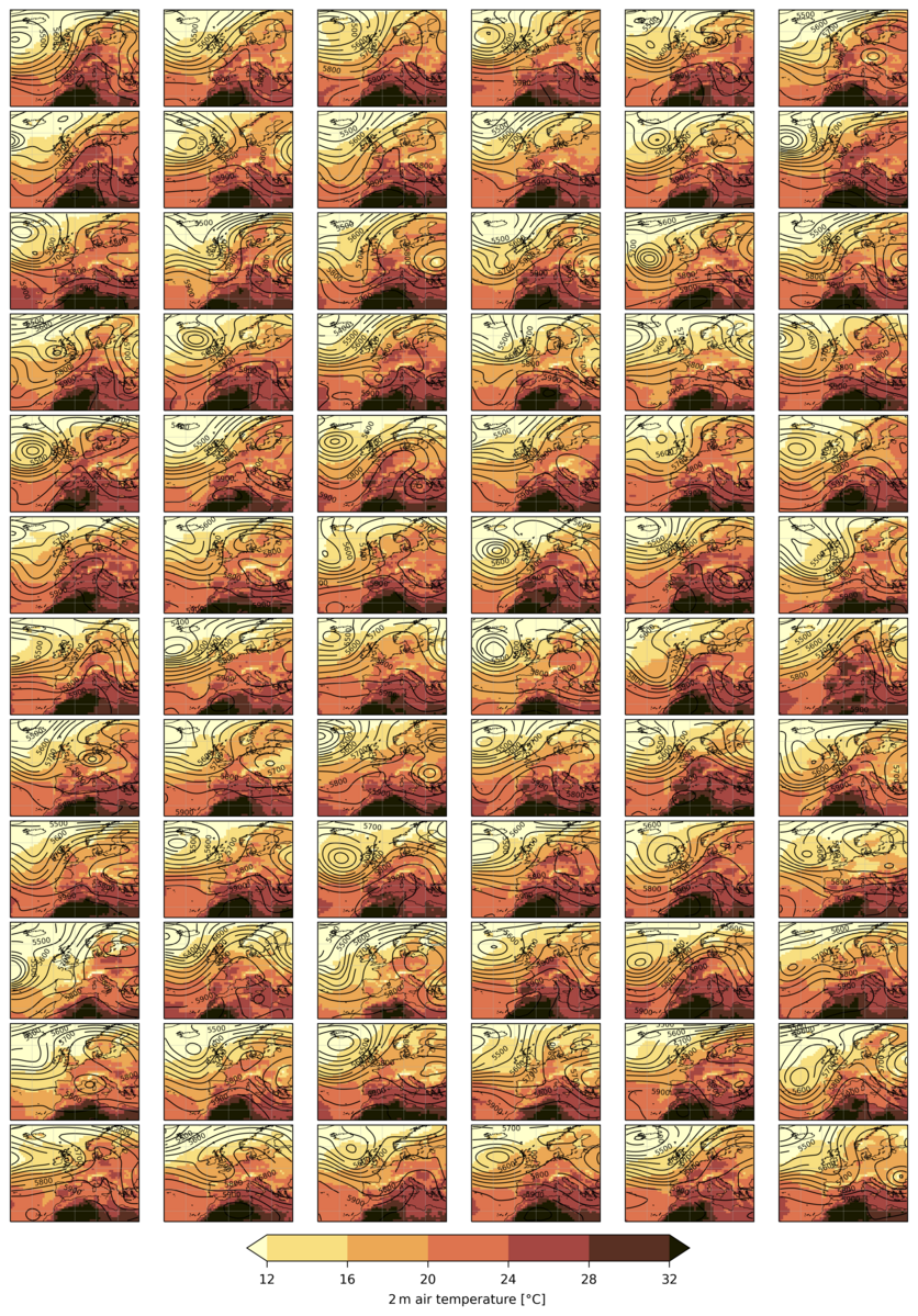
Figure B1 Analogues of the temperature event.

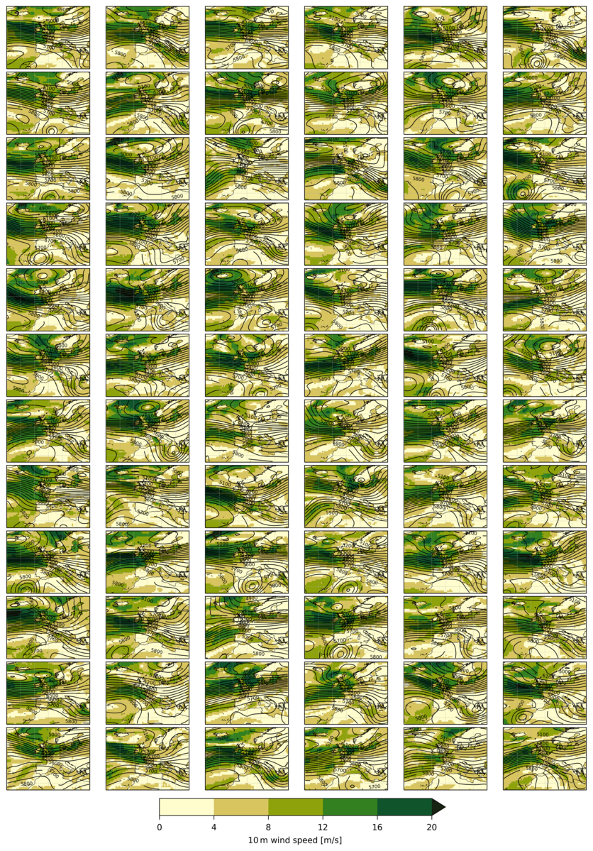
Figure B2 Analogues of the wind event.

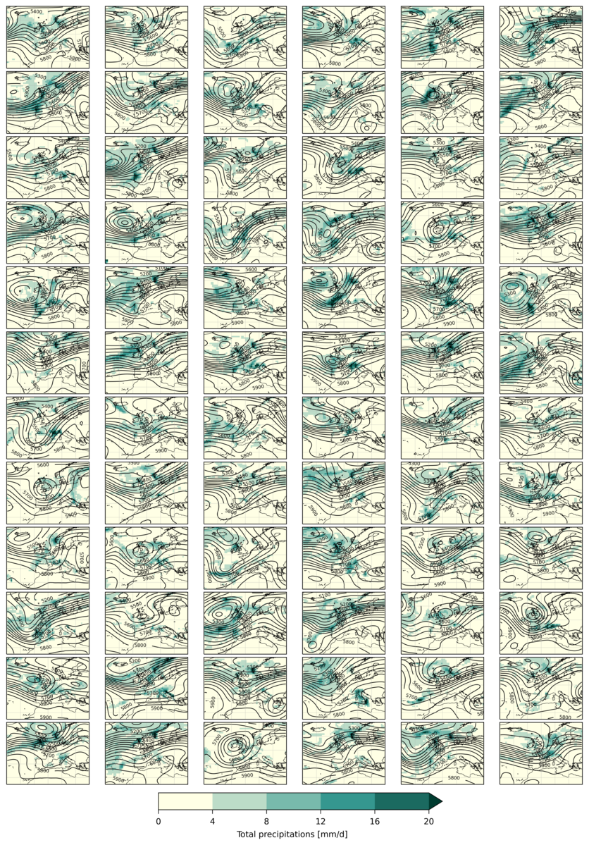
Figure B3 Analogues of the precipitation event.

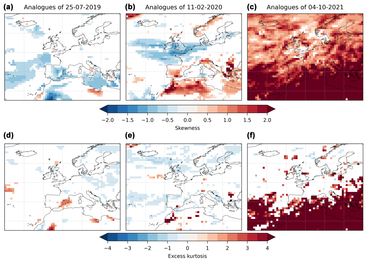
Figure B4 Empirical skewness (a–c) and excess kurtosis (d–f) of the analogue distribution of observables for the three events considered. Only the grid points where the skewness and excess kurtosis are significantly different than 0 are shown (see text for details).

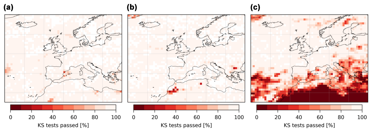
Figure B5 Kolmogorov–Smirnov tests. Proportion of Kolmogorov–Smirnov tests passed at the 5 % level over the 10³ resamplings at each grid point of the analogue distribution of (a) the 25 July 2019 temperature event, (b) the 11 February 2020 wind event and (c) the 4 October 2021 precipitation event.

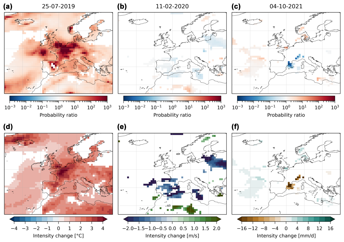
Figure B6 The same as Fig. 4 with 54 analogues.

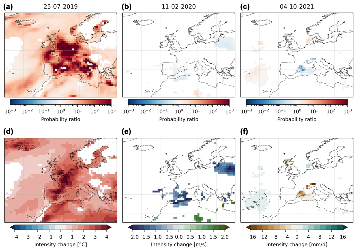
Figure B7 The same as Fig. 4 with 90 analogues.

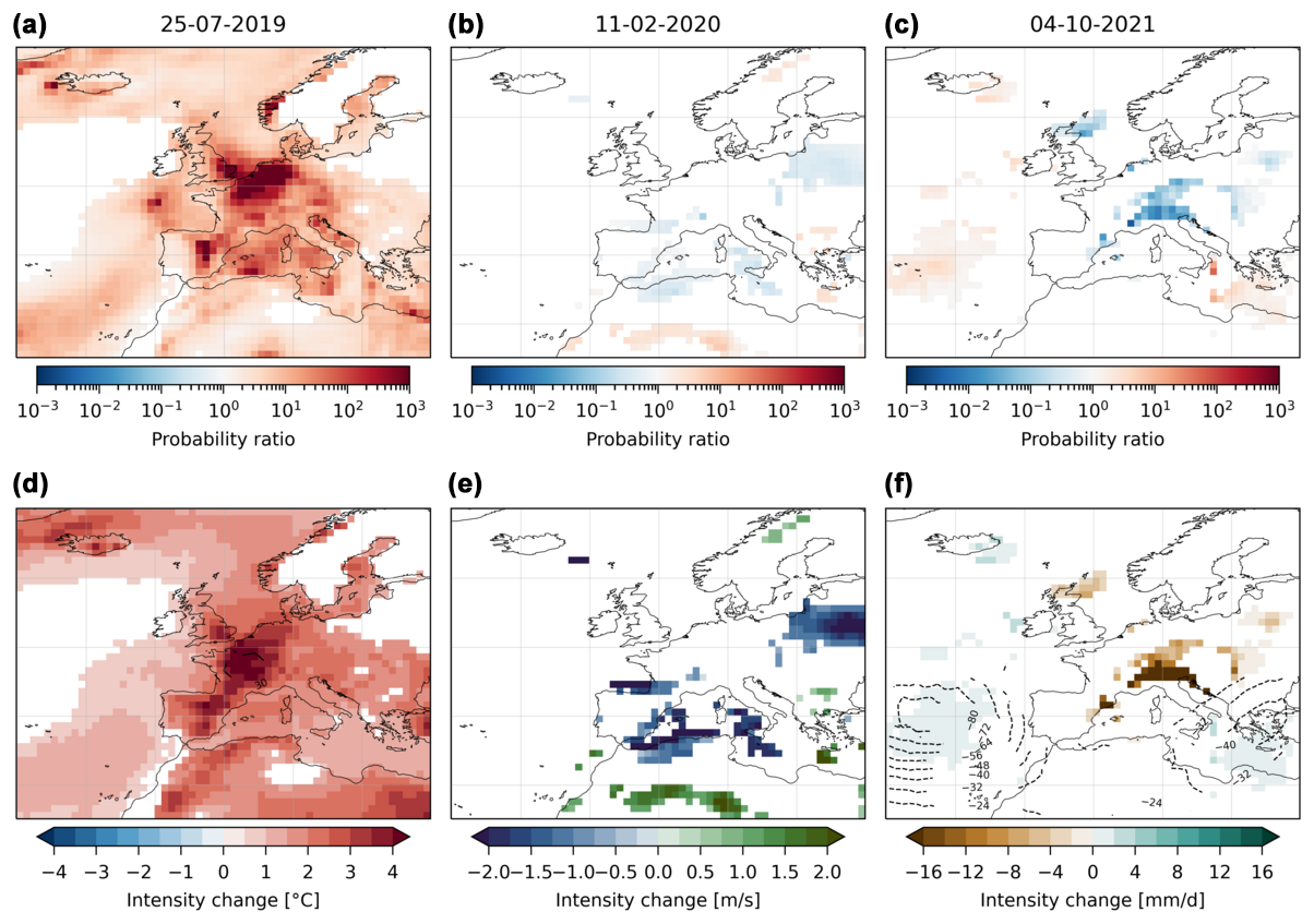
Figure B8 The same as Fig. 4 with an analogue domain larger by 3° of latitude and longitude at each edge.

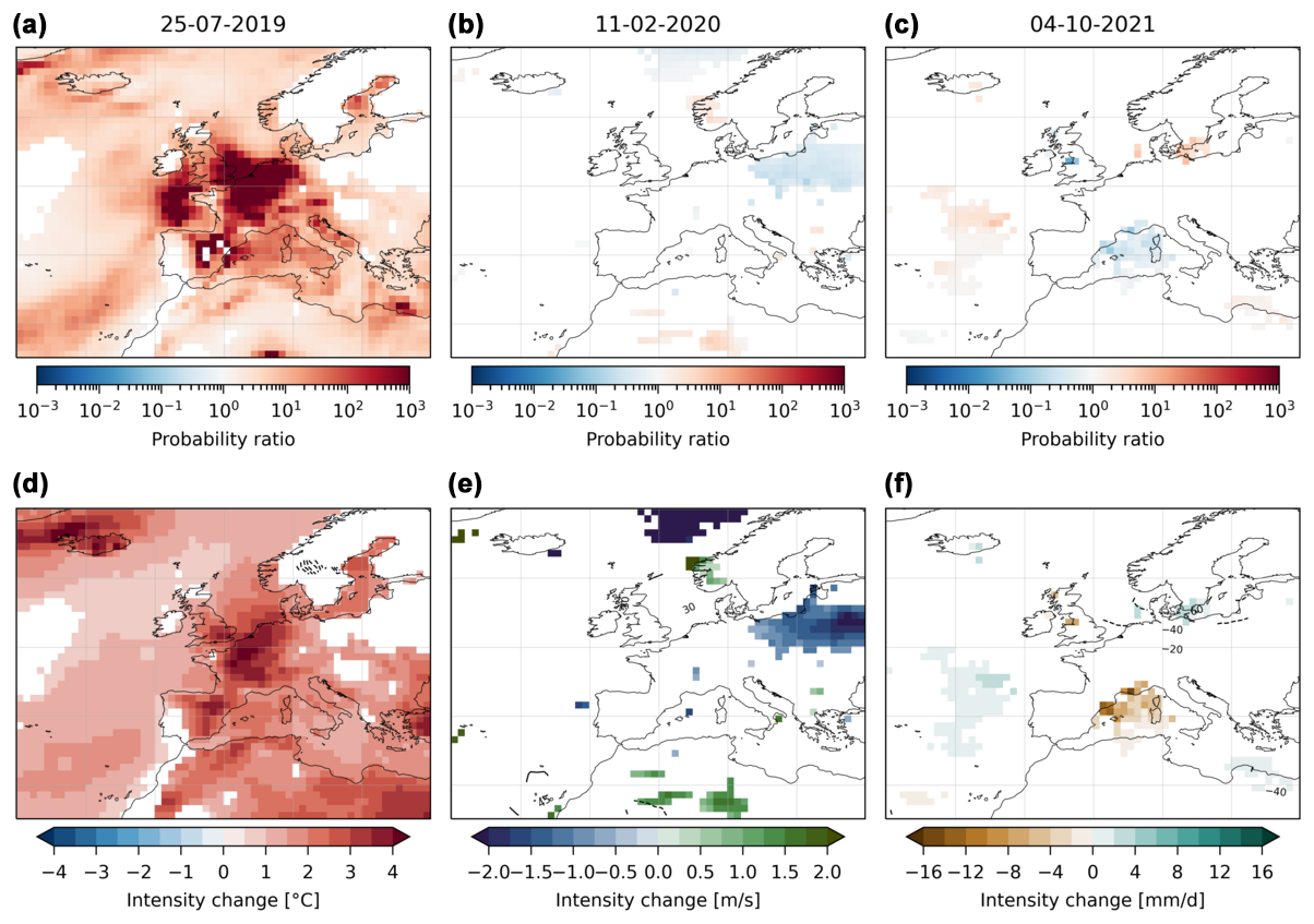
Figure B9 The same as Fig. 4 with an analogue domain smaller by 3° of latitude and longitude at each edge.