Forecast-based attribution of the role of stratospheric variability in weather extremes

Variability of the stratospheric polar vortex, particularly its dramatic breakdown during sudden stratospheric warming (SSW) events, has been linked to a number of surface weather extremes. However, attributing the role of stratospheric variability in a specific observed weather extreme, rather than an abstracted class of extremes, has proved highly challenging. Here we use an ensemble of subseasonal forecast simulations from 7 forecast systems participating in the Stratospheric Nudging and Predictable Surface Impacts (SNAPSI) project to carry out this task. By comparing the likelihood of extreme events in free-running forecasts to those with the zonal-mean stratospheric state nudged towards its observed or climatological evolution (while the troposphere is freely-evolving), we are able to calculate the changes in the risk and severity of extremes due to the occurrence, or non-occurrence, of an SSW. We focus on three case-study events: (i) the 2018 boreal SSW and subsequent Eurasian cold air outbreak and snowfall, (ii) the 2019 boreal SSW and subsequent North American cold air outbreak, and (iii) the 2019 austral near-SSW and subsequent Australian heat wave. Through an extreme value statistical analysis, we find in all three cases a significant stratospheric contribution to the risk of relevant weather extremes. In case (i), improving the SSW prediction by nudging as much as doubles the forecast risk of extreme Eurasian cold and UK snow. The differences in risk and severity between experiments nudged to the SSW and to climatology are relatively insensitive to the lead time before the cold air outbreak of case (i). By contrast, in case (ii) this difference only emerges at short lead times before the event, indicating a stratospheric influence on this event that is dependent on the tropospheric state. For case (iii) we find a stronger and more robust stratospheric impact on the severity of the Australian heat wave than on its risk, with the latter being highly sensitive to model bias. The methodology outlined here, including both the experimental design and the semi-parametric approaches for calculating risks, can be applied to attribute several other internal climate system drivers of extreme event risk.

1 Introduction

Following a severe weather event it is regularly asked what factors might have influenced its likelihood or severity. Of such factors, most interest has focussed on the role of anthropogenic climate change and there are now several hundred studies investigating the human influence on a wide range of extremes such as floods, droughts, heat waves, and storms (Stott et al., 2016; Otto, 2017, 2023; Seneviratne et al., 2021; Faranda et al., 2024). The field of extreme event attribution has also evolved to focus not just on weather events themselves, but also on their economic, human health, and ecosystem impacts (e.g. Mitchell et al., 2016; Perkins-Kirkpatrick et al., 2024). Relatively less attention has been paid to attributing the roles of internal climate system processes in extreme event probabilities. Here we will explore the role of one of these processes: polar stratospheric variability.

Methodologies for extreme event attribution can be broadly categorized into either probabilistic or storyline approaches (Noy et al., 2024). The probabilistic approach (Allen, 2003) evaluates changes in the likelihood of an abstracted class of event (such as annual maximum temperature) rather than a specific observed event (such as a heatwave). In contrast, storyline approaches focus on physical mechanisms and the change in magnitude of the particular event (Hoerling et al., 2013), which can be achieved through the use of circulation analogues (Shepherd, 2016), nudged model simulations (van Garderen et al., 2021; Sánchez-Benítez et al., 2022), perturbed reanalysis (Hawkins et al., 2023), or ensemble boosting (Gessner et al., 2021). Both methods have significant drawbacks. For instance, probabilistic approaches may give misleading results if the response of the abstracted class of event is not representative of the given observed event, while storyline approaches cannot determine changes to an event's likelihood, only its magnitude or a plausible range of magnitudes. These differing approaches have led to some seemingly contradictory conclusions (Otto et al., 2012; Hauser et al., 2017), and both are further limited by the inability of climate model simulations to capture the dynamics underlying many extreme events (Bellprat and Doblas-Reyes, 2016). Leach et al. (2021, 2024) proposed that an attribution approach based on medium-to-extended-range forecasts can help mitigate the above deficiencies. They showed that by varying the lead-time of forecasts the approach can move flexibly between a probabilistic framing (at long lead times) and storyline framing (at short lead times), and by using a successful forecast, the ability of the model to capture the given extreme event and its causes can be ensured.

We will here aim to adapt the forecast-based attribution methodology to investigate the role of stratospheric variability in three case studies of extreme weather events. The ensemble of subseasonal forecast experiments performed within the Stratospheric Nudging And Predictable Surface Impacts (SNAPSI) project (Hitchcock et al., 2022) will form the basis of our study. These consist of three core experiments: a standard free-running forecast ensemble, an ensemble in which the zonal-mean stratospheric state is nudged towards observations, and an ensemble in which the zonal-mean stratospheric state is nudged towards time-evolving climatology. In the typical framing of event attribution, we can view the two nudged ensembles as counterfactual scenarios in which the future evolution of the polar stratosphere can be predicted with either near-perfect skill or no skill (beyond that provided by climatology). By comparing extreme event probabilities in the counterfactual and standard forecasts, we will aim to answer two related questions:

1. What is the stratospheric contribution to the risk of a given extreme event?

2. How much can improved (or degraded) forecasts of the stratosphere improve (or degrade) the prediction of a given extreme event?

We will find that the answers to these questions depend on the event in question.

It is well established that polar stratospheric variability can be associated with a variety of extreme weather events, including cold air outbreaks, heatwaves, storms, and precipitation extremes (Domeisen and Butler, 2020). This link has been most clearly shown following sudden stratospheric warming (SSW) events (Baldwin et al., 2021), in which the stratospheric polar vortex rapidly breaks down in winter in the Northern Hemisphere and spring in the Southern Hemisphere, the impacts of which may propagate downwards and influence large-scale circulation patterns such as annular modes during the following two months. Several studies have used observational data to identify SSW impacts on specific surface extremes through analyses of weather regimes and dynamical processes such as wave propagation and reflection (Ayarzagüena et al., 2018; Matthias and Kretschmer, 2020; Lim et al., 2021). However, in such studies the lack of counterfactuals makes it impossible to quantify stratospheric impact on the risk or magnitude of a weather extreme, only to infer it qualitatively. Other studies have quantified a stratospheric impact through statistical causal inference (Kretschmer et al., 2018; Huang et al., 2021) or analysis of subseasonal-to-seasonal hindcasts (Spaeth and Birner, 2022; Rao et al., 2025), but these studies calculate an average over many SSW events, rather than the impact of a given event. SSWs vary widely in their tropospheric precursors, magnitude, and morphology Charlton and Polvani (e.g. 2007) so it is reasonable to expect that their impacts may be similarly varied. This expectation is further motivated by the wide range of surface weather events observed following SSWs. For instance, only around half of boreal SSWs are followed by European cold spells (Hall et al., 2023); likewise, many cold spells occur in the absence of significant stratospheric variability. In summary, while a mean downward impact of SSWs is well established, a quantitative measure of this impact on an event-by-event basis has remained challenging (see further discussion in the review of Butler et al., 2019).

Kautz et al. (2020) address this challenge with an approach that is similar to ours, using nudging of the zonal-mean stratospheric state to quantify its contribution to extreme weather risk. Specifically, they investigate the boreal major SSW of 12 February 2018 (one of the three case studies considered here), using the European Centre for Medium-range Weather Forecasts (ECMWF) Integrated Forecasting System (IFS) (one of the 7 models considered here). They find that the nudged forecasts initialized on 1 February 2018 have about a 9-times higher risk of a Eurasian cold spell than do the standard forecasts (absolute risks of 45 % and 5 %, respectively). As well as considering more case studies and forecast systems, we expand upon Kautz et al. (2020) in two other ways. First, we consider lead-time dependence by initializing all experiments at two dates for each case study. Second, we develop a semi-parametric approach to quantifying risk over a broad range of severity thresholds, in this case using extreme value distributions but easily applicable to other parametric families.

The nudging approach we use here is not limited to studies of SSWs and indeed has been applied to several other aspects of atmospheric variability, such as the quasi-biennial oscillation (Martin et al., 2021), as well as broader climate variability, such as sea-ice concentrations (Audette and Kushner, 2022) and sea-surface temperatures (Amaya et al., 2019). We therefore hope that the general forecast-based “process attribution” methodology described in this study can be adapted for quantifying the roles of other drivers of extreme events, which in turn can aid forecasters and risk analysts, and be used to compare anthropogenic and natural risks.

The remainder of this article is structured as follows. Section 2.1 gives a general description of the SNAPSI experimental protocol and describes the three case study events, while Sect. 2.2 explains the extreme value statistics approach. Section 3.1 then presents the attribution of extreme temperatures to stratospheric variability in each of the case study events. We then briefly investigate the attribution of extreme snow accumulation in Sect. 3.2; the aim being to illustrate how our methodology can be adapted for different variables, and, with this in mind, we limit our discussion here to the case of the southern UK and Ireland following the 12 February 2018 SSW case study. Finally, a discussion and conclusions of our results is given in Sect. 4.

2 Methodology

2.1 Experimental design and case studies

SNAPSI experiments consist of retrospective forecasts of three case study stratospheric polar vortex disruption events: the boreal major SSW of 12 February 2018 (which we refer to as SSWFeb18), the boreal major SSW of 2 January 2019 (SSWJan19), and the austral minor warming of 18 September 2019 (SSWSep19). SSWFeb18 and SSWJan19 are referred to as major warmings as the zonal-mean zonal wind at 10 hPa, 60° N reversed to become easterly, and their central dates are those on which the winds reversed. In contrast, this threshold (at 60° S) was not crossed for SSWSep19, although the zonal winds did decelerate rapidly; in SSWSep19 the central date is taken to be that of minimum zonal wind at 10 hPa, 60° S. For each case study we consider three experiments:

•  

  free A standard forecast ensemble, which is free-running following initialization.

•  

  nudged An ensemble in which stratospheric zonal-mean zonal wind and temperature are relaxed (i.e. nudged) to their observed evolution. The lower boundary of nudging is at 90 hPa, with a ramp to full strength at 50 hPa and above.

•  

  control An ensemble in which the relaxation is instead towards climatological mean values, which evolve in time following the seasonal cycle.

Table 1 Case study dates and spatial and temporal regions of interest for analyzing temperature extremes.

Swart et al. (2019)Richter et al. (2022)Danabasoglu et al. (2020)Voldoire et al. (2019)Williams et al. (2018)Walters et al. (2017)Koo et al. (2023)ECMWF (2023)

Table 2 Modeling centers and model names for the 7 forecast systems analyzed.

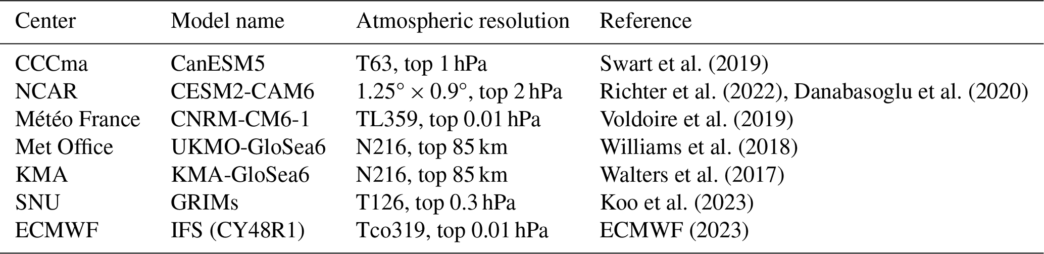
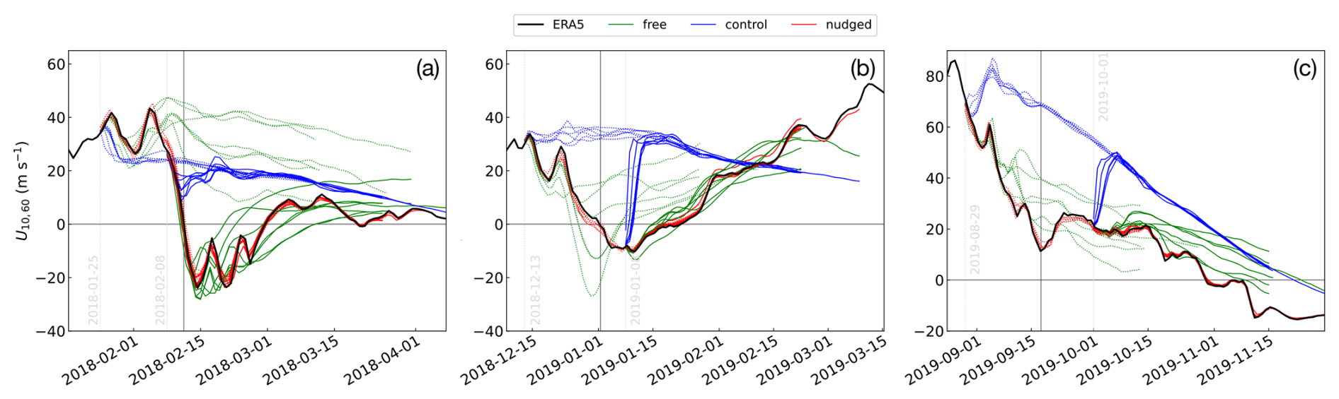
Figure 1 Stratospheric zonal-mean zonal wind evolution for the three case study events of SSWFeb18 (a), SSWJan19 (b) and SSWSep19 (c), in ERA5 reanalysis (black) and the three SNAPSI experiments (colors). Values are shown at 10 hPa and 60° N (a, b) or 60° S (c). Colored lines represent ensemble means of the 7 individual forecast systems in our analysis (excepting CanESM5 in panels b and c, for which the necessary data was not available). Dashed colored lines are used for the early initialization, solid lines for the late initialization. Solid vertical lines indicate the central date for each event and dashed vertical lines indicate the experiment initialization dates.

The observed evolution and climatology used for nudging are derived from the ERA5 reanalysis (Hersbach et al., 2020). Each experiment is initialized at two different dates for each case study (given in Table 1), and each consists of a 50-member ensemble, generated according to a methodology that varies by forecast system. For example, the IFS generates oceanic and atmospheric perturbations separately, the atmospheric component combining singular vectors and ensemble data assimilation. The same set of perturbations is applied to the free, control, and nudged experiments for fair comparisons. We analyze the output of 7 forecasting systems contributing to SNAPSI, which at the time of analysis had the data necessary (archived on the JASMIN facility; Lawrence et al., 2013) for our study available. These systems are listed in Table 2. A detailed description of the observed dynamical evolution of the three events and of the SNAPSI experimental design is given by Hitchcock et al. (2022), the impact of nudging on upward wave activity is investigated by Ayarzagüena et al. (2026), and an analysis of surface predictability within the SNAPSI experiments is given by Kim et al. (2026). However, to allow for interpretation of our later results, we illustrate the ensemble-mean impact of nudging on the polar mid-stratospheric zonal-mean zonal wind (at 10 hPa, 60° N/S) in Fig. 1.

SSWFeb18 (Fig. 1a) is seen to be poorly predicted by the free experiment at the early initialization, but well predicted at the late initialization. Indeed, for most models, the early initialization free experiment has a stronger polar vortex than the control. For SSWJan19 (Fig. 1b) , there is a smaller difference between early initialization free and nudged experiments, with some free models successfully predicting an SSW despite being initialized 20 d before it occurred. The late initialization for SSWJan19 comes after the SSW central date (this was chosen due to the longer lag between the SSW and surface anomalies, described further in Hitchcock et al., 2022), and the subsequent recovery of the polar vortex from this time is well predicted by the free experiments, with a large difference between these and control until early February. Similarly, for SSWSep19 (Fig. 1c), the differences between free and nudged experiments are smaller than with either of those and control, at least until November, indicating relatively good skill in the prediction of this event.

One motivation for the choice of these three case study events for SNAPSI was the range of surface weather extremes that were observed in the months following them. Here we will describe some key features of these events, with a focus on surface temperature extremes. In the period following SSWFeb18, from late-February to early-March 2018, negative Northern Annular Mode (NAM) and North Atlantic Oscillation (NAO) patterns were associated with anomalously cold temperatures extending over much of Eurasia (Lü et al., 2020). Concurrent weather events included snow over the UK (which we analyze in Sect. 3.2) (Galvin et al., 2019), as well as enhanced precipitation over Iberia (Ayarzagüena et al., 2018), ending an extended period of drought. An analysis of precipitation within SNAPSI experiments of SSWFeb18 is presented in Dai et al. (2025).

In contrast, during the period following the SSW of SSWJan19 the NAM remained near neutral, and temperature anomalies over Eurasia were comparably muted (Butler et al., 2020; Rao et al., 2020). However, more significant temperature anomalies occurred in North America, with an extensive cold spell in late January 2019 covering much of the Midwestern US and eastern Canada, with several daily cold temperature records being set in this region (Lillo et al., 2021). The dynamical evolution of this event has been described on synoptic scales as relating to an equatorward deviation of the extratropical jet stream as well as a tropopause polar vortex (Lillo et al., 2021), and on larger scales as linked to an Alaskan Ridge weather regime. However, in an analysis of SNAPSI experiments, Lee et al. (2025) find little stratospheric impact on the development of this weather regime. Indeed, by contrasting stratospherically- and tropically-nudged seasonal hindcast experiments, Knight et al. (2021) proposed a stronger tropical influence. Nonetheless, a direct attribution of the stratospheric role in the extreme cold spell has not been carried out.

SSWSep19 was the most significant disturbance to the austral stratospheric polar vortex since the major warming of 2002 (Lim et al., 2021). Following the central date of 18 September on which zonal mean winds at 10 hPa, 60° S reached a minimum (in the ERA5 data set), a negative Southern Annular Mode (SAM) pattern slowly descended from the mid-stratosphere, reaching the surface from approximately mid-October. The negative SAM pattern has been associated with hot and dry conditions over eastern Australia during late October to December, which in turn contributed to unprecedented destructive wildfires in the region (Lim et al., 2019, 2021). Stratosphere-troposphere coupling within the SSWSep19 SNAPSI experiments is discussed in detail by Feng et al. (2025), including an analysis of wildfire risk.

Motivated by these observed events we restrict our analysis to broad regions that capture the dominant observed temperature extremes for each case study (Fig. 2). For SSWFeb18 (Fig. 2a) this region matches exactly that of Kautz et al. (2020), for SSWJan19 (Fig. 2b) we select a region containing the most extreme cold anomalies identified by Lillo et al. (2021), and for SSWSep19 (Fig. 2c) we select a region containing the entire continent of Australia, in all cases considering only land areas for extreme temperature analysis. We also define a time window for each case study in which to determine temperature extremes. In doing so, we balance a desire to capture events similar in timing to that observed, while also not overly penalizing models that capture the magnitude of events well but have errors in timing. As such, we define periods that follow the central date of each SSW and bracket the most extreme temperatures observed in reanalysis by a margin of at least 5 d, or as wide as possible while remaining fully inside the common forecast period of both early and late initializations – with an exception of SSWSep19, where we extend the horizon beyond the range of the early forecast in order to bracket the highest extremes seen in the late ensemble. The SSWFeb18 ensembles bracket the extremes comfortably, but the SSWJan19 ensembles end before the greatest extremes and the late SSWSep19 ensembles start just barely before the greatest extremes, making them more sensitive to the choice of time interval. Expanded forecast horizons may be a goal for future experiments, and more systematic sensitivity analysis may be a goal for future attribution methods, but the current setup suffices to demonstrate our core methodology. The spatial and temporal boundaries of our below analysis are shown in Table 1, and Fig. 2 shows large and relatively spatially coherent anomalies of temperature extremes within the chosen regions, motivating their suitability for area-averaged analysis. The following spatial maps will focus only on the selected sub-regions.

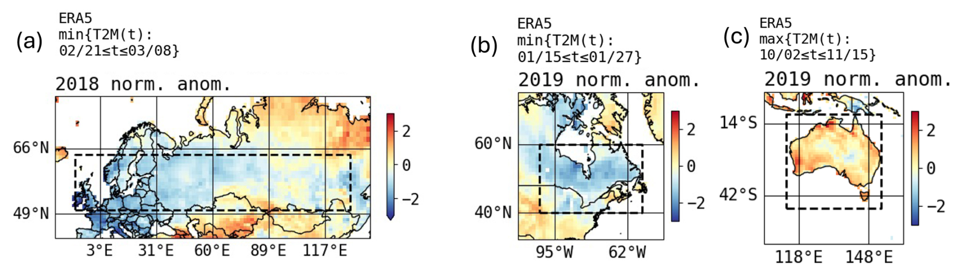
Figure 2 Anomalies of observed (ERA5) near-surface land temperature extremes for the three case studies, during their time windows of interest. Minima are shown for SSWFeb18 (a) and SSWJan19 (b), and maxima for SSWSep19 (c). Values are calculated relative to the climatological mean minimum (a, b) or maximum (c) temperature during the time window of interest at each grid point over 1979–2020, and normalized by the standard deviation over those years. The regions of interest for later area-averaged analysis for each case study are illustrated by dashed black boxes. Arrows on colorbars indicate values extending beyond the range shown.

2.2 Extreme value statistical analysis

For the purposes of our analysis we define severity as the spatially averaged and then temporally minimized (for SSWFeb18 and SSWJan19) or maximized (for SSWSep19) temperature. We notably consider absolute temperature, not anomaly, which is better connected to some major societal impacts (Sheridan et al., 2019), and on which several downstream impacts (e.g. snow) depend. Crucially, we quantify statistical responses to different nudging interventions using two quantities:

•  

  relative risk  (RR), a ratio of probabilities of exceeding some fixed severity, and

•  

  quantile shift  (QS), a difference in severity at some fixed exceedance probability.

These two quantities have complementary strengths and weaknesses that allow us to discern robust causal signals that partially overcome model bias.

We need some notation to summarize our statistical approach. Let g be an index for the data-generating system, either a forecast system or reanalysis, $\in \mathit{\{}\text{CESM2-CAM6},\mathrm{\dots },\text{IFS},\text{ERA5}\mathit{\}}$; e be an index for the experimental nudging protocol $\in \mathit{\{}\mathit{control},\mathit{free},\mathit{nudged}\mathit{\}}$ (not applicable to ERA5); i be an index for the initialization date $\in \mathit{\{}\text{early},\text{late}\mathit{\}}$ (not applicable to ERA5); t be a timestamp within the temporal window [A,B] in which the extremes can occur; m denote the ensemble member, $\in \mathit{\{}\mathrm{1},\mathrm{\dots },M=\mathrm{50}\mathit{\}}$ (for forecast systems) or $\mathit{\{}\mathrm{1980},\mathrm{\dots },\mathrm{2019}\mathit{\}}$ (for ERA5); and $S_{g,e,i,m}\left(t\right)$ be the intensity simulated by system g, experiment e, initialized from date i, as realized by the mth ensemble member, on day t. When g=ERA5, the subscripts (e,i) are not applicable, and are replaced by $(\cdot ,\cdot )$. For all three SSWs, S represents a land-only area-averaged 2 m temperature 〈T(t)〉 that is maximised daily over four six-hourly samples. For SSWFeb18 and SSWJan19, 〈T(t)〉 is multiplied by −1 before maximising, such that a more positive S represents colder temperature minima for these events, while a more positive S represents warmer temperature maxima for SSWSep19. The areas for averaging and the time intervals of interest are described in the previous section and shown in Table 1.

The format of the ensemble lends itself naturally to extreme value analysis with the method of block maxima (Coles, 2001). For each $(g,e,i,m)$, we define the severity as the peak intensity attained, and call it $S_{g,e,i,m}^{\ast }$:

$$\begin{array}{}\text{(1)}& {\displaystyle }{S}_{g,e,i,m}^{\ast }=\underset{A\le t\le B}{max}{S}_{g,e,i,m}\left(t\right),\end{array}$$

and fit a generalized extreme value (GEV) distribution to each ensemble $\mathit{\{}{S}_{e,i,m}^{\ast }:m=\mathrm{1},\mathrm{\dots },M\mathit{\}}$, using the method of probability-weighted moments, which tends to be more stable than maximum-likelihood for small sample sizes (Hosking et al., 1985). In other words, we consider $S_{g,e,i}^{\ast }$ to be a random variable whose cumulative distribution function (CDF) is defined for any value s as

$$\begin{array}{}\text{(2)}& \begin{array}{l}\mathbb{P}\mathit{\{}{S}_{g,e,i}^{\ast }\le s\mathit{\}}=F\left(s;{\mathit{\mu }}_{g,e,i},{\mathit{\sigma }}_{g,e,i},{\mathit{\xi }}_{g,e,i}\right)\\ \text{where}\\ F(s;\mathit{\mu },\mathit{\sigma },\mathit{\xi })=\left\{\begin{array}{ll}\exp [-(\mathrm{1}+\mathit{\xi }\frac{s-\mathit{\mu }}{\mathit{\sigma }}{)}_{+}^{-\mathrm{1}/\mathit{\xi }}]& \text{if}\mathit{\xi }\ne \mathrm{0}\\ \exp [-\exp (-\frac{s-\mathit{\mu }}{\mathit{\sigma }}{)}_{+}]& \text{if}\mathit{\xi }=\mathrm{0},\end{array}\right.\end{array}\end{array}$$

where the subscript + denotes the positive part of the expression, i.e. $x_{+}:=max(x,\mathrm{0})$. We will also refer below to the complementary CDF, or CCDF, which is the exceedance probability: $\text{CCDF}=\mathrm{1}-\text{CDF}$. The three parameters of the GEV $(\mathit{\mu },\mathit{\sigma },\mathit{\xi })$ are called the location, scale, and shape, respectively, which we abbreviate as a vector $\mathit{\theta }=[\mathit{\mu },\mathit{\sigma },\mathit{\xi }]$.

We emphatically acknowledge that the GEV is not a priori guaranteed to be appropriate, as this would require S^∗ to be the maximum of a set of random variables that is large in number (much more than 2 weeks), independent (unlike an ensemble of skillful forecasts), and identically distributed (devoid of any seasonal cycle). For this reason, we note that confidence intervals calculated with the GEV are likely to be underestimates. However, the GEV was found to capture the distribution of temperature extrema better than a Gaussian, and we use it only as a regularizing tool for the relatively small ensemble size of M=50. It is worth exploring other distribution choices more thoroughly – RR and QS are equally well-defined for any parametric family – but GEV was a natural, illustrative, and sufficiently fitting distribution family for the present demonstration.

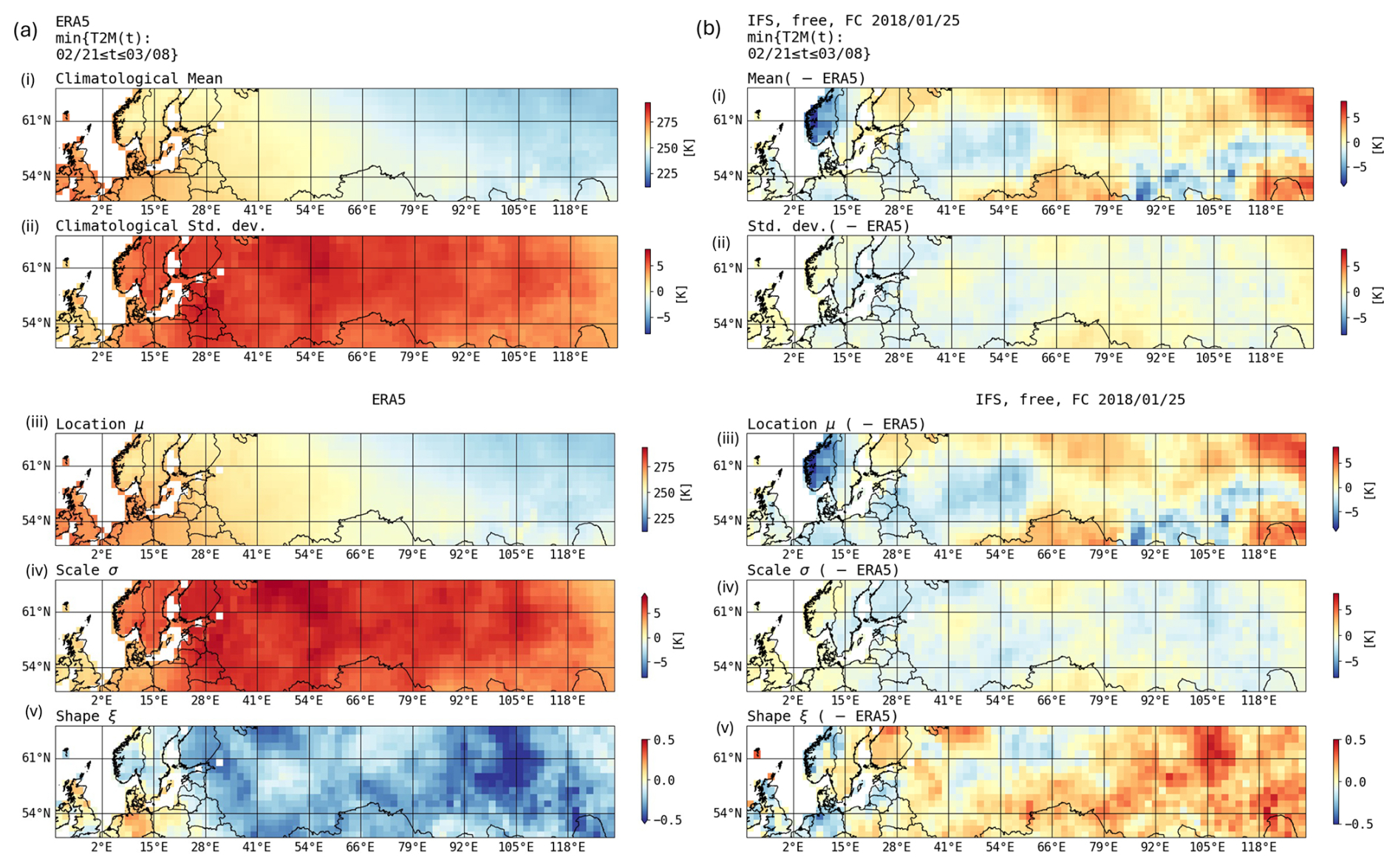
Figure 3 Statistical summary maps of surface temperature minima in the 16 d interval from 21 February. (a) Shows values over the “ensemble” of years from 1980–2020 in ERA5, (b) shows values from the IFS free ensemble for SSWFeb18 initialized on 25 January 2018 (early), as a difference relative to ERA5. Panels (i) show mean minima, (ii) standard deviation of minima, and (iii), (iv), and (v) show GEV parameters of location, scale, and shape, respectively. The similarity in spatial patterns between “normal” summary statistics (mean, standard deviation) with analogous GEV summary statistics (location, scale) affirms qualitatively that the GEV distribution is an appropriate parametric choice. The small differences in shown in panels (b)(i)–(iv), relative to corresponding panels (a)(i)–(iv), affirm qualitatively that the early forecast is not highly skillful, but statistically accurate with respect to climatology. Only the shape parameter ξ differs between ERA5 and IFS on the same order as its ERA5 value, which reflects is high sensitivity to the far tail.

To provide some context and aid the interpretation of the GEV results to follow, we provide in Fig. 3a a visual summary of distributional parameters derived from ERA5. Specifically, we consider the 16 d time interval (as in Table 1) from 21 February (ending on 7 or 8 March depending on the year, inclusive) each year from 1980 to 2019 as a different ensemble member (thus, M=40 in the ERA5 case). We compute the severity for each year, but for geographic illustration, the area averages are performed separately on each of the boxes tiling the domain (restricting the average to land pixels in all boxes). The mean severity and its standard deviation are shown in Figs. 3a(i,ii). Similar maps for SSWJan19 and SSWSep19, over their respective areas of interest, can be found in the Supplement.

We then fit a GEV distribution to each grid box, and plot the corresponding parameter maps in Fig. 3a(iii, iv, and v). The mean and GEV location have a clearly similar spatial pattern as do the standard deviation and GEV scale, confirming that these two GEV parameters represent what their names suggest. The shape parameter (Fig. 3a(v)) stands apart as a subtler-to-interpret, but highly influential parameter: a negative shape parameter imposes a bound on severity equal to $\mathit{\mu }-\mathit{\sigma }/\mathit{\xi }$, whereas a positive shape parameter allows for unbounded severity (see Eq. 2). The map indicates negative shape nearly everywhere, which is usually the case in GEV analysis of temperature extremes (Huang et al., 2016), despite the lack of any a priori bounds on surface temperature (Krakauer, 2024). Recent work has, however developed theoretical frameworks for upper bounds temperature in terms of geopotential height and soil moisture (Zhang and Boos, 2023; Li and Tamarin-Brodsky, 2026), and fruitfully applied this framework to data-driven statistical models (Noyelle et al., 2023, 2026).

We also illustrate equivalent distribution parameters for the 25 January 2018 initialization of the free ensemble of the IFS model in Fig. 3b. In general, the IFS model parameters are similar to those from reanalysis indicating that the ensemble is a close match to the climatology of extremes, but has little precision from this initialization date.

Although each grid box sub-region has its own severity distribution, the following quantitative risk analysis only considers full-region severities. Note the full-region GEV parameters are not simply the average of the sub-region GEV parameters, and a legitimate concern with the full-region average is lumping together many different regional climatologies, each of which merits a separate localized analysis. We deem the fits shown in the next section sufficiently good to provide robust results and establish the methodology, but a follow-on paper will quantify the extremal behavior across sub-regions and averaging scales.

3 Results

3.1 Extreme temperatures

We now aim to apply our statistical analysis to compare temperature extremes in the three SNAPSI experiments and in ERA5. Figure 4 summarizes full-region risk analysis on the IFS model for SSWFeb18. The left and right Fig. 4 panel groups (i and ii) display results for the early and late initializations, respectively, and the three rows display in order results for free, nudged, and control experiments. For each experiment (in red) and for ERA5 (in black) we show, on the left Fig. 4(i), the empirical risk function consisting of ordered pairs of points at ($\mathrm{1}/m$, T_(m)) for $m=\mathrm{1},\mathrm{\dots },M$, where T_(m) is the temperature (area-averaged and then time-minimized) of the mth ensemble member (or year, for ERA5) in order of increasing severity (i.e., the severity with a $\frac{\mathrm{1}}{m}$ chance, empirically, of being equalled or exceeded). We also plot as solid lines the GEV-fitted risk functions and their 50th percentile-bootstrapped confidence intervals (resampling with replacement 1000 times, re-calculating GEV parameters for each, and shading between the 25th and 75th percentiles). The ±1 standard deviation error bars on the GEV parameters themselves are indicated in the legends.

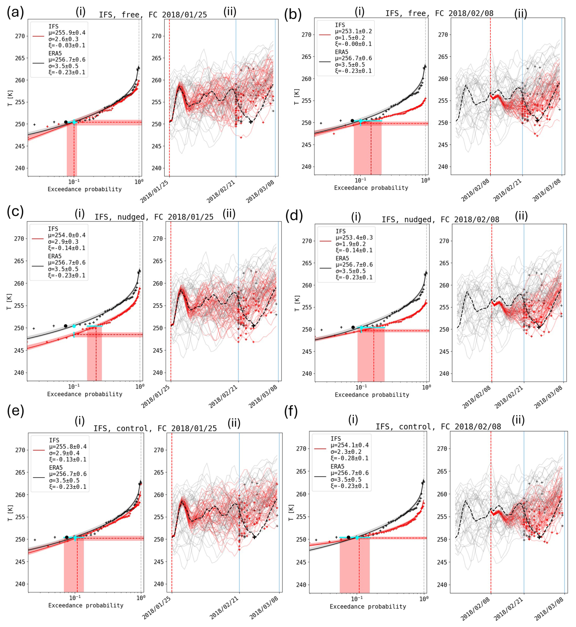
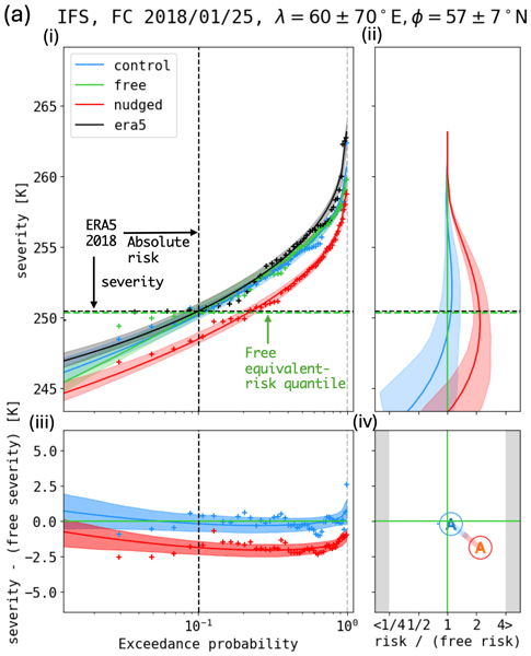
Figure 4 Forecast ensembles for SSWFeb18 produced by the IFS model: severity distributions (i) and timeseries (ii) of daily-minimum surface temperature, T, averaged over the full spatial region in Fig. 3. Left (a, c, e) and right (b, d, f) columns show early and late forecast dates. Top (a, b), middle (c, d), and bottom (e, f) rows show free, nudged, and control experiments. In more detail, panels (ii) display individual ensemble members' evolution as red timeseries, spreading out from the 2018 reanalysis (dashed black line) following the initialization date (red dashed vertical line). Gray lines show other years (“ensemble members” of ERA5) from the 1980–2020 record. Crosses (red for IFS and black for ERA5) mark the minimum of each member during the time span of interest (demarcated with blue vertical lines). These same minima are plotted as crosses in panels (i), versus the empirical exceedance probability (the probability of being even more extreme, in this case colder; e.g., for the 4th-coldest ensemble member out of 50, $\frac{\mathrm{4}}{\mathrm{50}}$ = 0.07). GEV fits and 50 % bootstrapped confidence intervals are overlaid. Dashed lines illustrate the calculation of absolute risk and equivalent severity: the observed severity (larger black crosses in panels ii) has, according to the ERA5 GEV fit ensemble, an exceedance probability given by the black curve's horizontal position at the same vertical level. We find the corresponding quantile in the early, free ensemble (cyan circle in panel a(i)) and fix this temperature as the reference against which all other forcing experiments are measured. The same cyan circle is plotted in panels (b)–(f).

We next explain how each forecast ensemble is boiled down to two numbers for later inter-model comparison. Starting at the ERA5 SSWFeb18 severity (∼ 250 K), we read off the horizontal position of the black curve to get a baseline risk level, regularized by the GEV fit, which we denote as AR₀. Then we draw a vertical line through this risk level and find the intersection with the early, free ensemble to get a temperature value, EQ₀, against which all other forcing experiments will be compared. The rationale is to substitute the observed ERA5 climatology with the model's early, free ensemble, which is very similar for IFS but is markedly different for some other models, in a form of bias-correction that treats the model as a “fixed-effect” and enables a clearer comparison between forcings, rather than a comparison between raw model fidelity. This baseline pairing is marked as a cyan dot. Then, for all six (forcing, initialization date) pairs, the corresponding ensemble's absolute risk (AR), shown by the vertical red dashed line, is the probability of exceeding EQ₀ (noting that, although we use the term “absolute”, AR remains conditional on the forecast initialization and any nudging). Similarly, each pair's equivalent-risk quantile (EQ) is shown by the horizontal red dashed line, as the severity at the same quantile as the baseline ERA5 value. In the (free, early) ensemble, these coincide with the baseline values EQ₀ and AR₀. Mathematically, following the notation in Sect. 2.2, let g denote the model, e denote the forcing experiment, and $i\in \mathit{\{}\mathrm{1},\mathrm{2}\mathit{\}}$ denote the initialization. We define for the (free, early) ensemble

$$\begin{array}{}\text{(3)}& {\displaystyle }\begin{array}{rl}{\text{AR}}_{\text{ERA5},\mathrm{2018}}& =\mathbb{P}\mathit{\{}{S}_{\text{ERA5}}^{\ast }\ge S_{\text{ERA5},\mathrm{2018}}^{\ast }\mathit{\}}\\ & =\mathrm{1}-F(S_{\text{ERA5},\mathrm{2018}}^{\ast };{\mathit{\theta }}_{\text{ERA5}})\end{array}\text{(4)}& {\displaystyle }{\text{AR}}_{g,\text{free},\mathrm{1}}={\text{AR}}_{\text{ERA5},\mathrm{2018}}\text{(5)}& {\displaystyle }{\text{EQ}}_{g,\text{free},\mathrm{1}}=F^{-\mathrm{1}}(\mathrm{1}-{\text{AR}}_{\text{ERA5},\mathrm{2018}};{\mathit{\theta }}_{g,\text{free},\mathrm{1}})\end{array}$$

where F⁻¹ is the inverse function of F, also known as the quantile function.

Then, for all (e,i) pairs,

$$\begin{array}{}\text{(6)}& {\displaystyle }{\mathrm{\text{AR}}}_{g,e,i}=\mathbb{P}\mathit{\{}{S}_{g,e,i}^{\ast }\ge {\text{EQ}}_{g,\text{free},\mathrm{1}}\mathit{\}}=\mathrm{1}-F(S_{g,\text{free},\mathrm{1}}^{\ast };{\mathit{\theta }}_{g\text{,e,i}})\text{(7)}& {\displaystyle }{\text{EQ}}_{g,e,i}=F^{-\mathrm{1}}(\mathrm{1}-{\text{AR}}_{g,\text{free},\mathrm{1}};{\mathit{\theta }}_{g,e,i})\end{array}$$

In the following, RR is a ratio of two absolute risks while QS is a difference in quantile. For example,

$$\begin{array}{}\text{(8)}& \begin{array}{rl}& \text{RR}={\displaystyle \frac{{\text{AR}}_{\text{IFS},\text{nudged},\mathrm{1}}}{{\text{AR}}_{\text{IFS},\text{free},\mathrm{1}}}}\text{and }\\ & \text{QS}={\text{EQ}}_{\text{IFS},\text{nudged},\mathrm{1}}-{\text{EQ}}_{\text{IFS},\text{free},\mathrm{1}}\end{array}\end{array}$$

measure two aspects of the response to nudging in the IFS model, initialized on 25 January 2018 (the early date, i=1). RR and QS have complementary advantages and drawbacks: RR is interpretable on a universal scale, no matter the event type or the physical units, but it may be zero or infinite in the presence of model bias. QS is always finite, but has physical units and characteristic magnitudes that depend, for example, on the spatial scale used for averaging. As we will find below, RR and QS should be interpreted with consideration for the underlying forecast skill of the event in question. For instance, if an event is well-predicted in free, nudging will be unlikely to influence its risk or severity (even if the event is stratospherically-influenced), hence the RR of nudged relative to free might be close to unity. In such a case, a better indicator of stratospheric influence might be the RR of control relative to free.

In order to further illustrate the calculation of the empirical risk function, the right-hand panels (a)–(f)(ii) of Fig. 4 show time series of intensity (daily region-averaged temperature) from the model ensemble and from all years of ERA5. The red and black crosses show the location of the minimum temperature during the period of interest, lining up with the locations of the points shown in the empirical risk function. The black dashed line shows the ERA5 time series for 2018. We see that the 2018 minimum temperature during this period, reached on 27 February, is the coldest on record for that day of year, and is the third coldest temperature reached over the whole period of interest. It is also apparent that in all 6 model experiment cases this observed severity lies within the ensemble spread, indicating the IFS model's ability to capture events of this magnitude. The same is true for SSWJan19 and SSWSep19, for which plots equivalent to Fig. 4 are shown in the Supplement.

At the earlier initialization, the risk function for all three experiments matches relatively closely that for ERA5 (Fig. 4, left column). This both illustrates that the forecasts from this initialization date have little precision beyond climatology (as previously noted in Fig. 3), and also that the “IFS climatology” – interpreted in the sense of an ensemble that has run just long enough to disperse, not a long multi-year single run – is relatively unbiased. The control climatology matches ERA5 climatology even better, which makes some heuristic sense because the control forcing makes the stratosphere match the ERA5 climatological mean by construction; however, nudging toward a single mean value does not imply matching the full distribution better, and might equally be expected to reduce the variance across members as a result of the lack of dispersion in the stratosphere and its influence on the troposphere. In other words, it is not obvious whether free or control experiments should better match the climatological distribution, especially when the climatological mean stratosphere is a sum over both SSW and non-SSW years and might not even be physically realizable. This is an important caveat for interpretation, and a potential improvement area for experimental design. For the later initialization (Fig. 4, right column), the IFS risk function is notably flatter than that of ERA5, indicative of greater forecast precision at the later initialization.

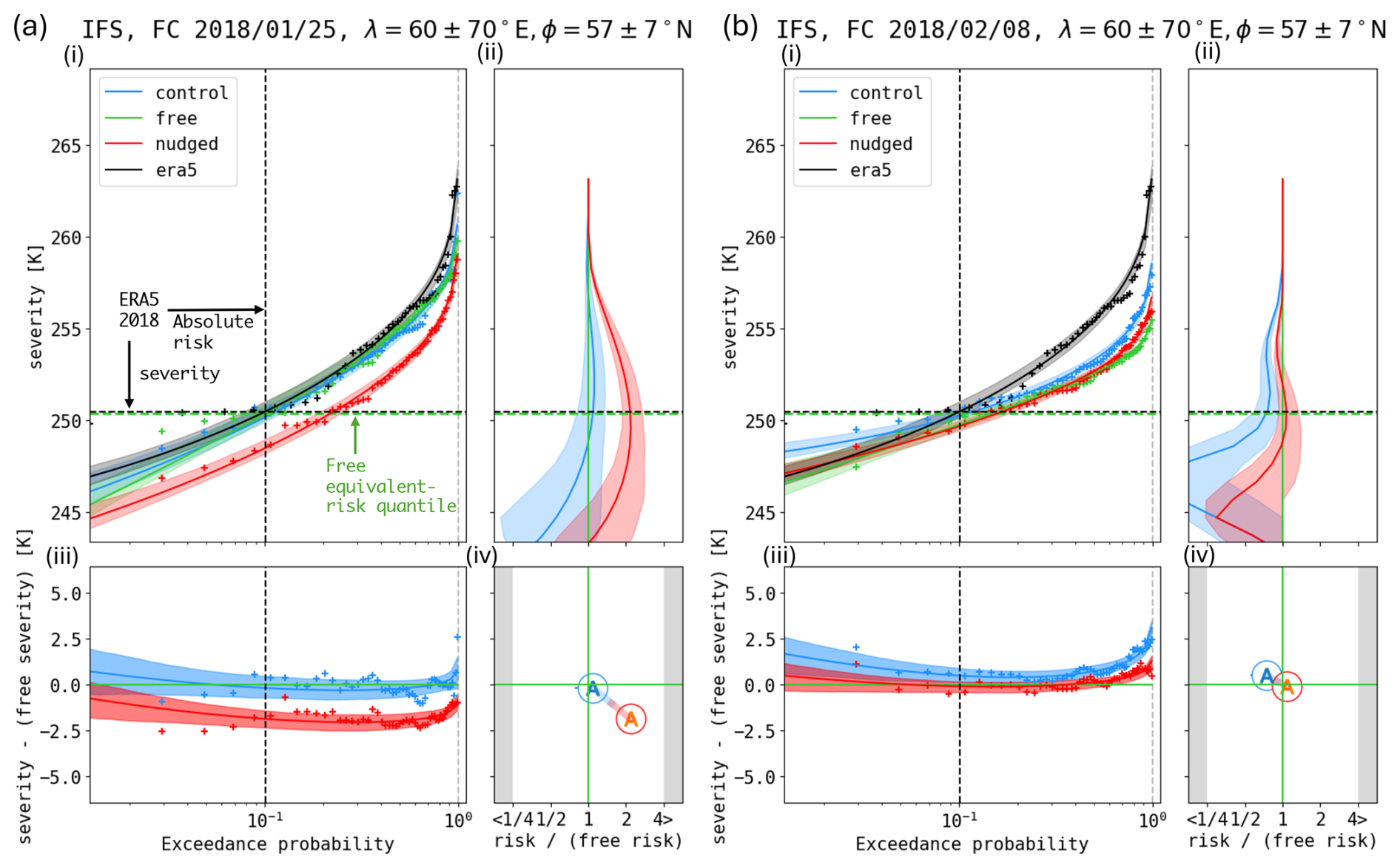
Figure 5 Summary of experimental effects according to IFS for SSWFeb18, for both early (a) and late (b) initialization dates. Panels (i) show severities S^∗ vs. risk, meaning the probability of an event of even greater severity. Crosses represent empirical risks, solid lines represent GEV-fitted risks, and shaded bands represent 50 % confidence intervals of GEV fits based on 1000 bootstrap resamplings. Panels (ii) show RR of the control and nudged distributions relative to free, as a function of severity. Panels (iii) show QSs of the control and nudged distributions relative to the free, as a function of risk, as well as empirical differences (available only when the two ensembles are equal in size). In other words, panels (ii, iii), respectively show horizontal and vertical differences between curves (or crosses) in panels (i). In panels (iv), we summarize each response as a single ordered pair (relative risk, quantile shift), by reading off intersections with the green dashed line in panels (ii) and the black vertical line in panels (iii). Any ratios < $\frac{\mathrm{1}}{\mathrm{4}}$ or > 4 would be clipped to the gray shading at the margins (see also Fig. 6).

The exceedance probabilities (CCDFs) for the three experiments, and both initialization dates of SSWFeb18 (retaining IFS as our example model), are overlaid in Fig. 5. RR is shown in panels Fig. 5(ii) as a function of severity, and QS is shown in panels Fig. 5(iii) as a function of exceedance probability, which are simply the horizontal ratio and vertical differences between curves in panels Fig. 5(i). The special thresholds given by ERA5 are marked by black dashed lines, and the equivalent-risk quantile in the early, free experiment is marked by green dashed lines. The intersection of these lines with the QS and RR curves, respectively give the nominal QS and RR values plotted as ordered pairs in panels Fig. 5(iv), and later used for inter-model comparison.

In the case of IFS, there is a clear and consistent pattern of influence: nudging toward observations both increases the RR and intensifies the QS relative to the control simulation, and the effect is larger for the earlier initialization. Figure 5iv captures this as a downward and rightward displacement of red relative to blue, which shrinks in magnitude at the later date. In the special case that ξ=0 for both experiments and the nominal severity S^∗ is far into the tail, RR and (log) QS are proportional, since the Gumbel distribution (GEV with ξ=0) is asymptotically exponential and thus the CCDF on a log scale is asymptotically linear:

$$\begin{array}{}\text{(9)}& \begin{array}{rl}& F(s;\mathit{\mu },\mathit{\sigma },\mathit{\xi }=\mathrm{0})\\ & =\exp [-\exp (-{\displaystyle \frac{s-\mathit{\mu }}{\mathit{\sigma }}}\left)\right]\sim \mathrm{1}-\exp (-{\displaystyle \frac{s-\mathit{\mu }}{\mathit{\sigma }}})\\ & ⟹\log (\mathrm{1}-F)\sim -{\displaystyle \frac{s-\mathit{\mu }}{\mathit{\sigma }}}\text{as}s\to \mathrm{\infty }.\end{array}\end{array}$$

However, in general RR and (log) QS are not necessarily proportional, especially if the severity of interest – nominally, the 250.5 K level achieved by ERA5 – is near the GEV-implied severity bound where the CCDF must curve sharply. We see this already in the late-initialized control experiment in Fig. 5b(i, ii), where the blue curve levels off substantially before exceeding (dipping below) the ERA5 severity, and its relative risk rapidly approaches zero. The implied lower bound on control severities is not far off, at $-(\mathit{\mu }-\frac{\mathit{\sigma }}{\mathit{\xi }})=-(-\mathrm{254}-\frac{\mathrm{2.3}}{-\mathrm{0.29}})$ = 246 K (the overall negative sign accounts for considering cold-side extremes). A small positive bias could easily have made the ERA5 severity impossible according to the control GEV fit, a conclusion which is physically reasonable but not well-described by relative risk. QS thus provides an important complementary viewpoint.

Let us point out some patterns in Fig. 5 which convey the effects of modulation of the stratospheric state on European cold extremes following SSWFeb18. In order from broad and robust to intricate and more uncertain:

• 1.

  Nudging the stratosphere toward the observed SSW intensifies surface cold extremes compared to relaxing the stratosphere toward its climatological mean. The RR (nudged/free) exceeds the RR (control/free) for the full range of severities in panels Fig. 5a and b(ii), and QS (nudged − free) is more negative than QS (control − free) in panel Fig. 5a and b(iii). Both of those differences exceed the error bar width at, and around, the 2018 ERA5 values, and for both early and late initializations. At the ERA5 severity of 250.5 K, the relative risk is a factor ∼ 2 larger for nudged than control at both initializations; at the ERA5 probability of ∼ 0.1, the nudged temperature is ∼ 2 and ∼ 0.5 K colder than the control temperature based on early (Fig. 5a) and late (Fig. 5b) initializations, respectively. IFS thus delivers a clear message that SSWFeb18 disposed the troposphere towards a stronger cold-air outbreak than the climatological average stratospheric evolution would have done.

• 2.

  Nudging towards observations (nudged) also intensifies the extreme event compared to the free simulation, but only for the early initialization. Started from the later date, nudging has a broadly neutral effect because the SSW is already well-predicted in the free simulation (Fig. 1a). Meanwhile, nudging toward climatology has a neutral effect when started early, and a moderating effect when started late.

• 3.

  The GEV fit does not capture all the important variation in severities, which is amplified in panels Fig. 5a and b(iii) and visible as non-random, oscillatory trends in empirical severities (crosses) about the GEV-derived CCDFs (solid lines). Possible culprits might include sub-asymptotic behavior (where GEV is not the best model), autocorrelations across space and time, and deterministic imprints of common perturbations between control and free ensembles, as suggested by the similar pattern of scatter between blue and red crosses. In other words, the underlying distribution may be a mixture of those representing different physical processes, and so not fully captured by a single GEV.

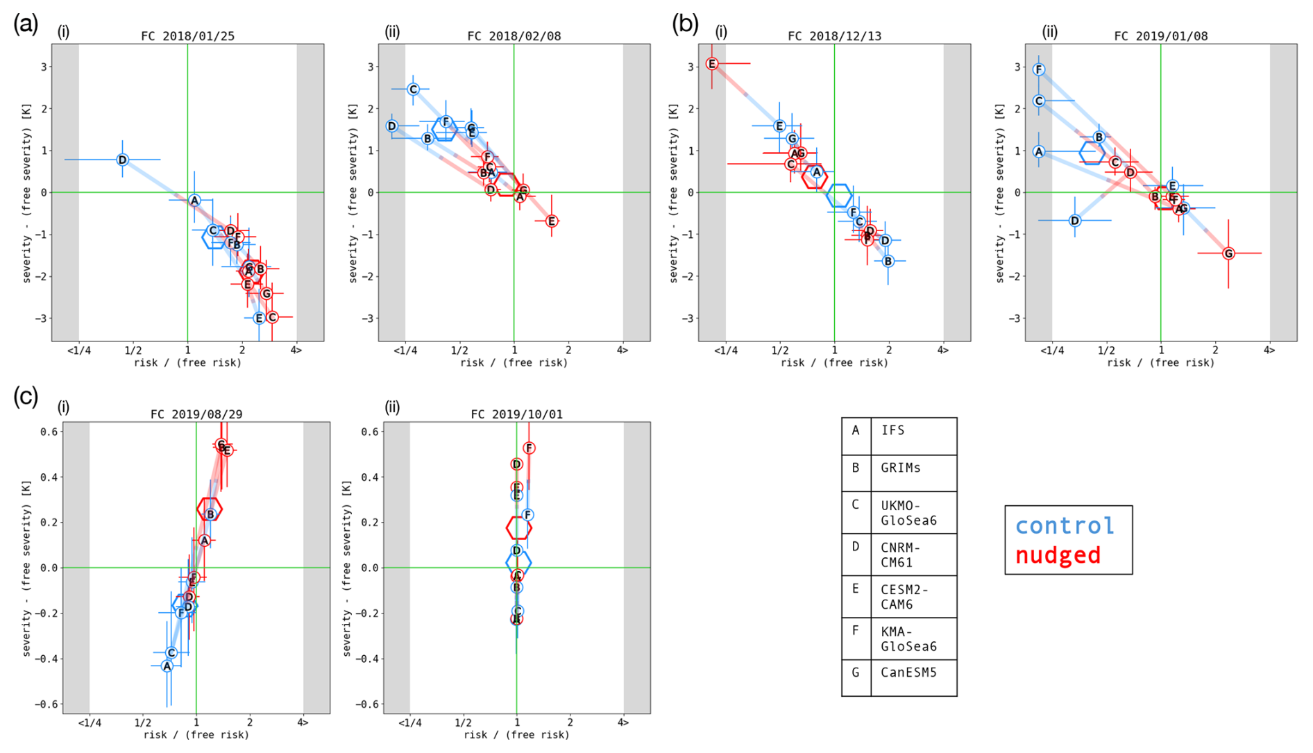
Figure 6 Relative risks (RRs) and quantile shifts (QSs). For each case study of extreme temperatures (a: SSWFeb18, b: SSWJan19, and c: SSWSep19), for each initialization date (i: early and ii: late), for both forcing experiments (blue: control and red: nudged), and for each model (represented by circled letters, as per the key), the response to forcing is plotted in a two-dimensional space (RR, QS), both defined with respect to the free experiment as a baseline (Fig. 5a and b(iv) are the IFS-only versions for SSWFeb18). Thick shaded lines connect each model's free and control responses, to help see patterns in the direction of influence. Multi-model means are represented by the large hexagons, with the relative-risk component being a geometric mean (taken in log space).

Figures equivalent to Figs. 3–5, but for SSWJan19 and SSWSep19 can be found in the Supplement. For a succinct inter-model comparison of the three events, Fig. 6 summarizes these results for all three case studies (Fig. 6a: SSWFeb18, Fig. 6b: SSWJan19, and Fig. 6c: SSWSep19) and both initialization dates (i: early and ii: late), reporting for each model and date only the slice of the RR curve evaluated at the ERA5 severity, and the slice of the QS curve evaluated at the ERA5 GEV-fitted risk, as in Fig. 5a and b(iv). Error bars are 50th percentile-bootstrapped confidence intervals, as in Fig. 5. A multi-model mean, taken by averaging these two metrics after calculating them for each model, is also shown (large hexagon). The results for SSWFeb18 are relatively consistent across models, and so with those already discussed for IFS. The early initialized nudged experiments of all models have both increased risk (on average by a factor of about 2) and increased severity (on average by about 1–2 K) compared to free forecasts. The control experiments also show (with the exception of CNRM-CM6-1) an increase in risk and severity, though this is more modest, both on average and in most individual models. This might be explained by the fact that the stratospheric polar vortex is on average stronger in the free than the control experiments for the early initialization (Fig. 1a). At the later initialization, nudged experiments show little change (relative to free) in RR or QS, but control experiments show a consistent reduction of both by factors of about $\mathrm{1}/\mathrm{2}$ and 1.5 K, respectively.

The other two case studies are not as consistent across models and initializations, which highlights the diversity of SSWs: in surface impacts, in lead-time dependence of predictability, and in how robustly models represent them. In SSWJan19 late nudging towards climatology reduces the risk of cold air outbreaks over North America, and reduces their severity – the same as in SSWFeb18, with close similarity between Fig. 6a and b(ii) – but, unlike SSWFeb18, early nudging or relaxation to climatology in SSWJan19 has a small average effect and little consistency of sign among models. This sensitivity of the stratospheric effect to lead-time suggests state-dependence, a point that will be expanded upon in Sect. 4.

In SSWSep19, nudging towards observations appears to consistently strengthen the severity of hot conditions over Australia in terms of QS, but a smaller signature is seen in terms of RR. Especially for the late initialization, most RRs are not significantly different from unity, because most ensemble members of most models exceed the threshold identified from the (free, early) experiment (see Fig. S6 in the Supplement for the example of IFS), which is the very reason why RR is an erratic indicator and QS is needed to extract some meaningful signal. Also, in this case it is not as fair to compare early with late initializations because we chose a target time horizon (through 15 November) that extends beyond the range of the early forecast (which ends 14 October; see Fig. S5). Nevertheless, the larger QS for nudged than for control in the early initialization forecast, which is consistent between models, reveals the role of the SSW in increasing the temperatures over Australia in the first half of October 2019. The same result in the late initialization forecast further confirms that the SSW did play a role in the observed extremes during spring 2019.

In aggregate, we affirm the original hypothesis of the SNAPSI project with regard to surface extremes – that the SSWs significantly affect the predicted risk of extreme surface temperatures – in only some cases: SSWFeb18 (both early and late initializations), SSWJan19 (the late initialization only) and SSWSep19 (both initializations, but with incomplete information for the first, which are truncated too early for a completely fair comparison). The other effects are mixed, and warrant a great deal of further exploration, in particular the geography of impacts, which a following paper will explore.

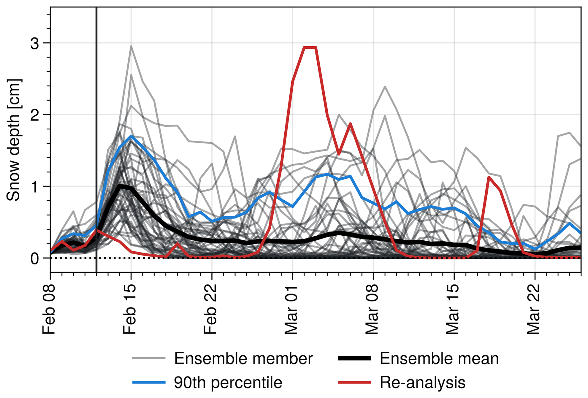
Figure 7 Snow depth averaged over the southern UK and Ireland ([10° W, 2° E] × [50° N, 55° N]) in 2018, in ERA5 (red), IFS free ensemble members (gray). The IFS ensemble mean is in black and the 90th percentile in blue. The vertical black line indicates the SSW onset date.

3.2 Extreme snow

As an illustration of how the attribution methodology described above might be adapted to other variables besides temperature, we will briefly describe an analysis of snow extremes. Specifically, we focus on SSWFeb18 and the extreme snow that accumulated over much of the UK during late February–March 2018 (Galvin et al., 2019). Figure 7 shows snow depth averaged over land in the box [50° N, 55° N] × [10° W, 2° E], constituting the southern UK and Ireland. ERA5 reanalysis (in red) shows a maximum close to 3 cm being reached in early March. The 25 January 2018 initialized free forecasts from IFS are shown in gray. No ensemble members simulate an accurate timing and magnitude of this snow event, although there is some indication of an increased probability of high snow in early March (shown by a local maximum in the 90th percentile of the ensemble, in blue). The model also predicts a snow event in mid-February of much greater magnitude than in reanalysis, such that on 14 February all ensemble members have snow depth greater than ERA5.

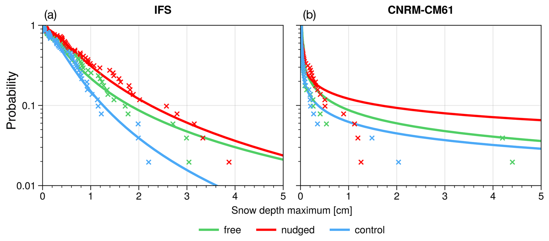
Figure 8 Empirical risk functions, calculated as in Fig. 4a(i), but for maximum snow depth over the southern UK and Ireland, for IFS (a) and CNRM-CM6-1 (b). Values are shown for the 25 January 2018 initialization, with the same time window as in Table 1. Crosses indicate risk calculated from individual ensemble members, solid lines show GEV fits.

Figure 8 shows exceedance probabilities (for the same time window as in Table 1) of snow depth for the early initializations of two example models; IFS and CNRM-CM61. As could be seen in the snow depth time series, very few ensemble members simulate snow accumulation maxima close to or above the observed values of about 3 cm (about $\mathrm{5}/\mathrm{50}$ ensemble members in IFS and $\mathrm{2}/\mathrm{50}$ in CNRM-CM61). Second, the parametric fits are much poorer than those for temperature, a problem that is again greater for CNRM-CM61. We hypothesize that the poor GEV fit is due to a very large number of ensemble members having zero (or close to zero) snow during the whole evaluation period (as can be seen in the time series of Fig. 7). Nonetheless, it is apparent that there are systematic differences between the three experiments, with nudged giving generally higher exceedance probabilities than free, and control generally lower probabilities.

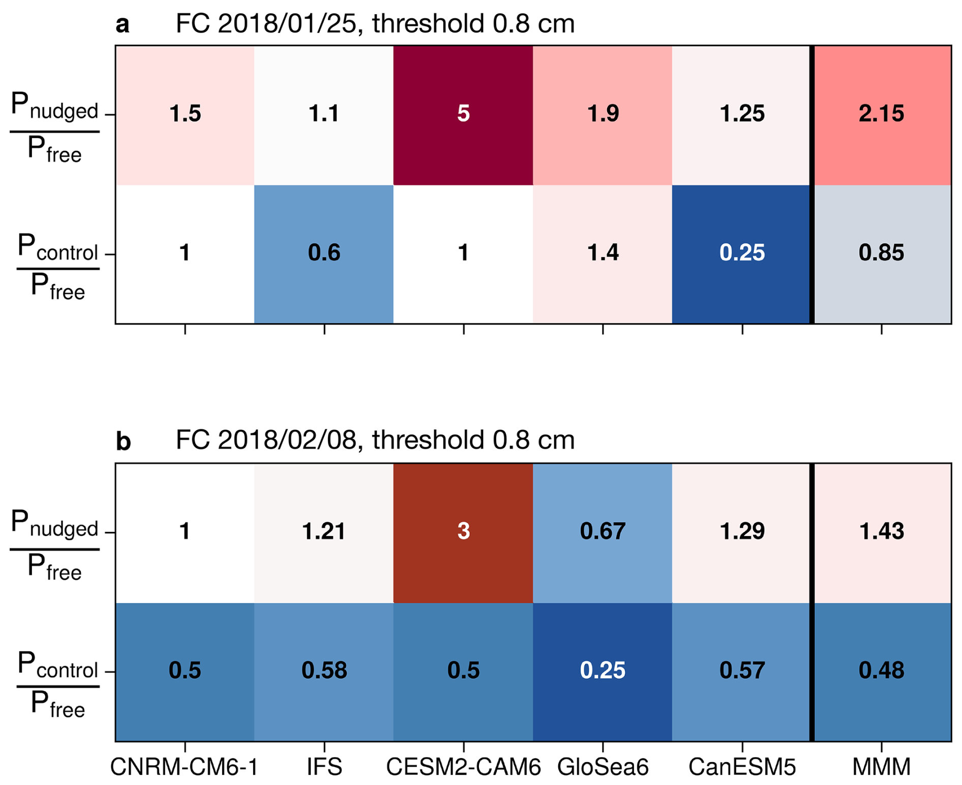
Figure 9 Non-parametric RR calculated for 5 models (for which appropriate snow depth data was available) for southern UK and Ireland snow depth, with a threshold of 0.8 cm. Values are shown for early (a) and late (b) SSWFeb18 initialization dates, and a multi-model mean, calculated by averaging RR after calculating for individual models, is also shown. The version of GloSea6 shown is UKMO-GloSea6.

Given the poor parametric fits for snow we illustrate a simpler approach to calculating RR based purely on counting ensemble members and not on the GEV fits. Here, RR is simply the ratio of the number of members exceeding a given threshold, and is shown for nudged/free and control/free in Fig. 9 for 5 of the 7 models for which appropriate snow depth data was available, as well as a multi-model mean. We choose a threshold of 0.8 cm, which is much lower than the observed maximum near 3 cm; this is to avoid large errors or infinite RR caused by dividing by a small number (or zero) when few ensemble members exceed the threshold. An inability to quantify RR for thresholds near or beyond the ensemble spread is an inherent drawback of this non-parametric approach. However, Fig. S7 shows RR (as a multi-model mean) for thresholds from 0.2 to 1.8 cm, with qualitatively similar results across this range.

Although there is significant spread between models, some consistent results emerge. First, in all models, improving the stratospheric forecast by nudging to reanalysis early (when the SSW is poorly predicted; Fig. 1a) increases the risk of snow (by on average about a factor of 2), while the sign of the effect of nudging late is mixed among models. Second, nudging to climatology early has a small and inconsistent sign effect, while nudging to climatology late (when the SSW is well predicted) reduces the risk of snow in all models (by on average about a factor of 0.5). These results are broadly consistent with our findings for temperature (noting the larger geographical region considered for temperature), and indicate that, in terms of inter-model consistency, there is a robust impact of the 2018 SSW on the probability of UK and Ireland snow accumulation.

4 Conclusions and discussion

We have compared ensembles of free-running and nudged (to either an observed event or observed climatology) subseasonal forecasts to understand the role of stratospheric variability in the risk of surface weather extremes. Specifically, we set out to address (1) the attribution of extreme event risk to stratospheric variability, and (2) the extent to which improved or degraded stratospheric forecasts impact extreme event prediction. For both tasks we have found that our results depend on the particular case study considered.

For SSWFeb18 we see that an improved stratospheric prediction at an early initialization increases the predicted cold-spell risk by about a factor of 2 and severity by about 2 °C, while degrading the stratospheric forecast at a later initialization decreases the Eurasian cold-spell risk by a similar factor (although there is significant spread among models). Hence we can conclude that the role of the stratosphere in this event remains significant and approximately constant throughout this time period, with a fraction of attributable risk given by $\text{FAR}=\mathrm{1}-\mathrm{1}/\text{RR}=\mathrm{1}-\mathrm{1}/\mathrm{2}=\mathrm{0.5}$ (e.g. Lott and Stott, 2016). In other words, approximately half of the total risk of the cold spell can be attributed to the stratospheric evolution. In this case, while an improved stratospheric forecast at an early initialization increases the predicted risk, the forecast at the late initialization is sufficiently accurate that further improvement by nudging has little impact. We find similar results for UK and Ireland snow, with a relatively consistent stratospheric influence on event risk throughout. Our RR is smaller than that of Kautz et al. (2020), who used the same region and time period and found a RR for a Eurasian cold spell of about 9 for IFS in their nudged relative to control experiments, higher than we find for any model. A potential explanation for our weaker signal is that Kautz et al. (2020) nudge to persistence rather than climatology in the stratosphere, with forecasts initialized on 1 February, which would result in a vortex stronger than the SNAPSI control simulation (e.g. Lee et al., 2025). Kautz et al. (2020) also nudge to the full stratospheric evolution, not just the zonal mean, which may further enhance the stratospheric impact. Interestingly, the FAR of 0.5 that we find here is close to that found by Spaeth and Birner (2022) for the mean impact of SSWs on Arctic Oscillation extremes.

For SSWJan19 our results are more initialization dependent. At the early initialization, nudging has little impact on the North American cold-spell risk. However, at the late initialization (in this case 6 d after the SSW onset), degrading the stratospheric forecast by nudging to climatology consistently reduces the predicted risk (by about half) and severity (by about 1 °C) of the cold spell. It is noteworthy here that, unlike Eurasia, mean temperature anomalies following SSWs are small or positive within our North American region (Domeisen and Butler, 2020), and the Alaskan Ridge weather regime that accompanied the cold spell is not, on average, favored by a weak stratospheric polar vortex (Lee et al., 2019). In an analysis of weather regimes in SNAPSI experiments, Lee et al. (2025) found that the early-initialized nudged forecasts for SSWJan19 erroneously favor a negative NAO pattern, more typical of the “canonical” SSW response (seen in SSWFeb18), with little effect on North American weather regimes. However, for the late-initialized forecasts, the Alaskan Ridge regime is well-predicted, likely developing due to a tropical teleconnection rather than a stratospheric influence (Knight et al., 2021). In this case, control experiments see a decreased Alaskan Ridge probability relative to free or nudged (Lee et al., 2025), a result that is consistent with a strong vortex instead favoring a Pacific Trough regime (Lee et al., 2019). In summary, these results suggest that while the SSWJan19 SSW did not drive the weather regime responsible for the North American cold-spell, it did play a role, once this regime had developed, in its persistence. This is an example of state-dependence in the stratospheric influence on event risk.

For SSWSep19, the severity of the Australian spring 2019 heat wave is higher in nudged than control in almost all models for both initializations. However the change in RR between experiments is seen here to be a much more variable metric among models than is QS for the early initialization, and for the late initialization RR is near 1 for all models. We suggest that this is due to the greater sensitivity of RR to bias, as well as the different time windows for analysis of the early and late initializations of this event, meaning that the late initialization extremes are warmer in part due to the warming seasonal cycle. Note, however, that we only infer any potential bias from our results for this single case study (e.g. noting the large difference in ERA5 and IFS empirical risk functions in Fig. S6), and we are not able to fully evaluate model bias. Nonetheless, the more robust effect of nudging increasing heat wave severity (positive QS) is consistent with other studies of the impact of weak vortex events on Australian temperature (Lim et al., 2019) and of this event in particular (Lim et al., 2021; Feng et al., 2025). Specifically, studies have linked weak vortex events to a negative Southern Annular Mode, which in turn is associated with warm and dry, and therefore wildfire-conducive, conditions over eastern Australia. Indeed, in an analysis of SNAPSI experiments Feng et al. (2025) have found an increase in wildfire risk index in nudged relative to control simulations, a result that is likely related to the increased heat wave severity found here, but that may also have contributions from extreme dry and windy conditions that we do not analyze. Our ability to attribute the Australian heatwave event is limited by the 45 d length of the SNAPSI experiments which, even for the later initialization, do not extend into December, when the most extreme heat wave occurred. Revisiting this event with longer hindcast experiments would be a valuable exercise.

More generally, we have aimed for this paper to illustrate a “process attribution” methodology that can be used to attribute the contribution of aspects of internal climate variability to extreme event risk. In doing so, we have learned three main lessons. First, we have found the S2S models analyzed here to be generally capable of simulating events at the observed severity, which verifies their suitability for studying drivers of the risk of these events, in common with recent climate change attribution studies (Leach et al., 2021, 2024).

Second, we have seen that GEV distributions provide a good fit to temperature extremes, both in their geographic pattern and when spatially averaged. This allows for a parametric approach to be taken, reducing the sensitivity to individual ensemble members. We have analyzed the impact of stratospheric nudging on extremes via two metrics: RR (the fractional change in risk for a given severity) and QS (the absolute change in severity for a given risk). While these two have generally been seen to change together (i.e. an increase in RR being accompanied with a negative QS for cold spells), this is not generally true due to the nonlinear nature of GEV distributions, and for SSWSep19 we saw significant changes in QS without accompanying change in RR. We have also seen that RR, being a ratio, is a much more erratic metric, showing less consistency among models. We therefore propose viewing extreme event changes under the lens of both metrics.

Third, we have seen that our parametric approach may not be suited to all variables. In our analysis of snow depth, a variable with very different characteristics from temperature, we have seen that the GEV distributions do not provide a good fit (Fig. 8). In this case, we illustrate a non-parametric approach, based simply on counting ensemble members exceeding a given threshold. This has the disadvantage of being highly sensitive to individual ensemble members, and being unable to assess risk near or beyond the ensemble spread. It may be possible to adapt the parametric approach to snow and other variables; for instance, by fitting a different distribution, or by removing zero values from the ensemble before fitting.

A significant limitation of our analysis is that we have not been able to carry out bias correction of SNAPSI simulations, due to a lack of historical hindcast simulations in equivalent model versions. This limitation is ameliorated somewhat by the fact that we are analyzing differences or ratios between nudged, free and control simulations, rather than absolute values; however, since risk functions are non-linear, this does not remove the effect of bias. Indeed, as discussed above, we suggest that larger Australian temperature biases may be responsible for the small relative risk changes seen in SSWSep19. A thorough evaluation of model bias would include not just free-running hindcasts but also nudged and control hindcast experiments.

Some caution must also be exercised in interpreting our results as fully capturing the risk attributable to stratospheric variability. S2S models vary in their strength of stratosphere-troposphere coupling relative to reanalysis (Garfinkel et al., 2025). Indeed, the majority of models under-estimate the correlation between stratospheric polar vortex strength and Eurasian surface temperature (Garfinkel et al., 2026), which might tend to lead to a reduction in the level of attribution. Furthermore, the control experiment, which involves nudging to the zonal-mean climatological-mean state, is not necessarily a realizable state of the atmosphere, so may not be suitable as a counterfactual that represents a lack of SSW. A more realistic counterfactual might instead nudge each ensemble member towards a randomly-selected observed non-SSW period from the same time of year. Finally, although we have identified several robust signals, our results are quite noisy. Large uncertainties are mostly a result of the 50-member ensemble size of SNAPSI simulations, which, being comparable to the number of years of reanalysis, is only just able to capture risks of the size evaluated here. Future work with larger ensemble sizes, a greater range of SSW (and other) events, and including nudging over other regions (e.g. the tropical troposphere) to capture the effects of other remote drivers of risk would be a valuable extension of this work. A more explicit linking of simulated extreme events to physical mechanisms such as weather regimes would lend further robustness to our statistical analysis. Finally, an extension of value to risk analysts would be to understand and attribute the stratospheric contribution to not just weather extremes, but also their societal impacts. Motivated by this, Rupp et al. (2025) investigate mortality impacts of SSWFeb18 using SNAPSI experiments, and we plan for a following paper to also investigate energy system impacts.