Global characterisation of the vertical temperature anomaly structure of heat extremes over land in ERA5

The formation of surface heat extremes is usually described in terms of surface processes and upper-level dynamics. However, their full vertical temperature profile contains additional essential information about the involved processes. So far, it is an open question whether heat extremes are associated with characteristic vertical temperature anomaly profiles and, if they exist, how they vary across the globe. In this study, we globally and systematically classify vertical temperature anomaly profiles during annual maximum 2 m temperature events (TXx) using a k-means clustering approach. After normalising and scaling the anomaly profiles, we find three clusters whose global distribution closely follows the polar, mid-latitude, and tropical climate zones. The three clusters capture key structural differences of heat extremes. Within the tropical cluster, positive temperature anomalies during TXx events are vertically confined to the (often deep) boundary layer and intensify progressively in the days leading up to the event, while the upper troposphere is not deviating from its climatological mean. The mid-latitude cluster also exhibits bottom-heavy temperature anomalies, which, however, extend throughout the full troposphere, showing a strong vertical coupling during TXx events. In the polar cluster, the events are characterised by deep tropospheric positive anomalies, accompanied by the erosion of the near-surface inversion layer, resulting in a shallow layer of particularly strong temperature anomalies near the ground. These results show that while multiple physical mechanisms can generate a heat extreme, at first order, the median normalised and scaled temperature anomaly profiles during heat extremes are similar to each other within a given climate zone. Deviations from the cluster median during individual TXx events mainly come from the variability between TXx events rather than the variability between the median profiles at different grid points. Finally, the normalised and scaled temperature anomaly profiles of the most extreme TXx events are particularly well represented by the grid point's median profile for all TXx events, suggesting a typical dynamic of the most extreme heat events.

1 Introduction

Particularly in the tropics, the average vertical temperature structure of the atmosphere is set by an equilibrium between surface sensible and latent heat fluxes, leading to convection, and radiative cooling by outgoing long-wave radiation: a state known as radiative-convective equilibrium (Manabe and Strickler, 1964). Frequent convective events and mixing by gravity waves result in vertical temperature profiles that closely follow the moist adiabats with weak horizontal gradients (Nicholls et al., 1991; Emanuel et al., 1994; Vallis, 2017). In the mid-latitudes, the atmosphere is more stable with respect to convection compared to the tropics, i.e., the lapse rate (defined as $-\mathrm{d}T/\mathrm{d}z$) is smaller than the moist adiabatic lapse rate, as both convection and large-scale dynamics (e.g., baroclinic instability) contribute to the upward transport of energy (Vallis, 2017). Finally, polar regions are in a radiative-advective equilibrium as these regions feature cold and ice-covered surfaces with high albedo, preventing the formation of diurnal convection and leading to near-surface temperature inversion layers with strong vertical temperature gradients that decouple the surface from the large-scale flow aloft (Cronin and Jansen, 2016; Nygård et al., 2017; Shahi et al., 2020). At synoptic time scales, vertical temperature profiles can deviate significantly from their climatological mean, especially during extreme surface temperature events (e.g. Hotz et al., 2024). Therefore, vertical temperature profiles result from the coupling between large-scale dynamics and surface processes, and can thus provide insight into the mechanisms controlling surface extremes, such as extreme precipitation or heat events. For example, the intensity of extreme precipitation events has been shown to scale according to their vertical temperature (and wind speed) profile (O'Gorman and Schneider, 2009). However, little is known about vertical temperature profiles during heat extremes and how they are set by different physical mechanisms.

Temperature anomalies arise from three different categories of physical processes (e.g. Röthlisberger and Papritz, 2023): horizontal transport of air from climatologically warmer or colder regions (advection), adiabatic warming and cooling by vertical motions, and diabatic warming and cooling by various processes including turbulent surface fluxes, radiation, and latent heat release. In mid-latitudes, surface heat extremes are typically associated with an upper-level anticyclonic flow (Xoplaki et al., 2003; Stefanon et al., 2012), originating either from blocked anticyclones, recurrent Rossby wave patterns, or subtropical ridges (Pfahl and Wernli, 2012; Röthlisberger et al., 2019; Sousa et al., 2021). Upstream diabatic heating helps to form and maintain these upper-level anticyclones and blocks (Pfahl et al., 2015; Steinfeld and Pfahl, 2019; Zschenderlein et al., 2020). In the lower troposphere, the anticyclonic flow promotes near-surface warming via adiabatic warming through subsidence and advection of warm air masses either from crossing climatological temperature gradients or from anomalously directed flows (e.g. Bieli et al., 2015; Santos et al., 2015; Zschenderlein et al., 2019; Röthlisberger and Papritz, 2023; Mayer, 2025). Beyond large-scale dynamical processes, near-surface temperatures are strongly governed by land–atmosphere interactions in the planetary boundary layer (PBL). Over warm surfaces, sensible heat fluxes can warm the near-surface air, and their relative intensity compared to latent heat fluxes depends on the soil moisture content and, thus, the evapotranspiration regime – energy-limited or soil-moisture-limited (Seneviratne et al., 2010; Schwingshackl et al., 2017). The stationarity of blocking situations can sustain heat extremes (Röthlisberger and Martius, 2019), during which soil drying in soil-moisture limited regions enhances sensible heating, further intensifying near-surface temperatures (Fischer et al., 2007; Lorenz et al., 2010; Seneviratne et al., 2010; Pappert et al., 2025). Aside from local sensible heating, the advection of heat from upstream dry regions can also exacerbate near-surface temperatures (Schumacher et al., 2019).

Outside the mid-latitudes, a different mix of processes generates near-surface heat extremes (Röthlisberger and Papritz, 2023). In equatorial regions with dry surface conditions, enhanced sensible heat fluxes lead to a stronger warming at the surface and a larger lapse rate in the lower troposphere than over wet surfaces, whereas the mid- and upper tropospheric lapse rate remains approximately moist adiabatic across the tropics due to weak horizontal temperature gradients (Sobel and Bretherton, 2000; Joshi et al., 2008). Heat extremes therefore occur when moist convection is suppressed, either due to reduced soil and PBL moisture (Byrne, 2021; Zhang et al., 2021; Costa et al., 2022) or entrainment of dry air (Duan et al., 2024). In terms of the near-surface temperature anomaly decomposition by Röthlisberger and Papritz (2023), this leads to high diabatic contributions. Consequently, surface temperature anomalies over tropical land reflect variations in downward shortwave radiation, soil moisture availability, and surface energy partitioning (e.g. Schwingshackl et al., 2017; Byrne, 2021; Costa et al., 2022; Wu et al., 2023). In contrast, in polar regions, poleward transport of warm and moist air can lead to heat extremes, including over Antarctica (Wille et al., 2024). Furthermore, as indicated by major melt events in Greenland (Hermann et al., 2020), heat extremes in polar regions can also be associated with upper-level anticyclones, which give rise to poleward warm advection along their western flank, and subsidence within the anticyclones (e.g. Papritz, 2020; Röthlisberger and Papritz, 2023). Blanchard‐Wrigglesworth et al. (2023) and Wille et al. (2024) also found that during the intrusion of warm and moist air leading to the heatwave in eastern Antarctica in 2022, the near-surface temperature inversion was eroded due to increased moisture and incoming long-wave radiation.

Despite our growing understanding of heatwave dynamics across the globe, the exceptional intensity of several recent events remains difficult to explain within current theoretical frameworks. One extraordinary intense heatwave occurred in the Pacific Northwest region in 2021 (e.g. Philip et al., 2022; White et al., 2023). While such a heatwave was virtually impossible according to classical statistical approaches based on historical data (Philip et al., 2022), long simulations suggest that even though such heatwaves are possible, they are very rare (McKinnon and Simpson, 2022; Bloin-Wibe et al., 2025). Recent studies have investigated vertical temperature profiles during heat extremes, hypothesising that the vertical structure of temperature may be important for explaining the intensity of recent surface heat extremes (e.g. Neal et al., 2022; Schumacher et al., 2022; Zhang and Boos, 2023). Miralles et al. (2014) showed in case studies over Europe that heat can accumulate within the PBL over multiple days during heat extremes: Heat preserved in the nocturnal residual layer during the night can re-enter the PBL the following day, allowing the near-surface temperatures to rise progressively in the course of several days. Zhang and Boos (2023) proposed that, similar to the tropics, the surface intensity of mid-latitude heat extremes is constrained by a moist convective limit controlled by upper-level dynamics. Following this argument, the theory has been extended for cases where convective inhibition or dilution by entrainment suppresses or weakens moist convection (Duan et al., 2024; Li and Tamarin-Brodsky, 2026), and also for dry convective cases (Nicolas and Hotz, 2026). Indeed, record-breaking high temperature anomalies occurred in the mid- and upper-troposphere, for example, during the Pacific Northwest 2021 heatwave. These anomalies were produced by strong advection and latent heating within a warm conveyor belt of an upstream cyclone (Schumacher et al., 2022; Oertel et al., 2023; Hotz et al., 2024). They then enhanced vertical stability and favoured the build-up of extreme near-surface temperatures (Neal et al., 2022; Zhang and Boos, 2023). Hotz et al. (2024) showed that three recent record-shattering heatwaves featured vertically deep but bottom-heavy temperature anomalies. However, the magnitude of these anomalies and their underlying processes varied strongly between the cases. Similarly, during blocking situations, Brunner et al. (2016) and Nabizadeh et al. (2021) found vertically deep positive temperature anomalies, e.g. during the Russian heatwave in 2010. Lhotka and Kyselý (2024) classified vertical temperature profiles during heat extremes in Europe and found several types depending on the vertical extent of the positive anomalies and referred to them as near-surface, lower-tropospheric, higher-tropospheric, and omnipresent temperature anomalies.

So far, no global studies have systematically investigated the structure of vertical temperature profiles during surface heat extremes, and therefore, our knowledge of the vertical structure relies on a few case studies and specific regions. In this study, we document the vertical temperature structure during surface heat extremes on a global scale and investigate its variability between regions and individual events. Specifically, we address the following questions:

1. Are there representative vertical profiles of temperature anomalies during TXx events across the globe, and how do these profiles vary geographically (Sect. 3.1 and 3.3)?

2. How does this vertical profile develop in the days before and after the TXx events (Sect. 3.2)?

3. How well do the representative profiles agree with median profiles during TXx events at individual grid points, and how variable are the profiles across events (Sect. 4)?

4. Is the structure of the vertical temperature anomaly profiles during the most intense TXx events similar to profiles during average TXx events (Sect. 5)?

In the following, we introduce the data and methods used in this study in Sect. 2, and then address the questions introduced above in three results sections. Finally, we present our conclusions in Sect. 6.

2 Data and methods

This study is based on the global reanalysis dataset ERA5 provided by the European Centre for Medium-Range Weather Forecast (ECMWF). We expect the vertical structure of heat extremes to be well-captured in ERA5, as these events are large-scale phenomena whose vertical structures are generally well-represented in the reanalysis (Hersbach et al., 2020). The ERA5 reanalysis has important limitations in its representation of the boundary layer and near-surface vertical structure. The near-surface maximum temperatures are generally underestimated in ERA5 (Lopes et al., 2024). Furthermore, Nicolas and Hotz (2026) have shown that ERA5 can have biases in super-adiabatic layers in elevated arid areas compared to observational soundings. Additionally, ERA5 tends to overestimate the surface latent heat flux over land, indicating that the partitioning of surface energy to heat and drought stress is biased (Martens et al., 2020), which can influence the boundary layer vertical structure. However, based on regional studies, the correspondence of ERA5 to observational soundings is relatively good (e.g. Cao et al., 2026). We use ERA5 in three-hourly temporal and 0.5° × 0.5° spatial resolution on the lowermost 98 hybrid sigma–pressure levels (extending to about 30 hPa) from 1951 to 2023 (Hersbach et al., 2020; Soci et al., 2024). We focus on land grid points only, assuming differences in the physical processes of heat extremes and, therefore, in their vertical structure, over land and ocean, and define land grid points as those that are more than half covered by land.

2.1 Normalised temperature anomalies

At each grid point (i,j) and vertical hybrid sigma–pressure level k, we compute the temperature anomaly T^′ by removing the climatological temperature T_clim from the absolute temperature T:

$$\begin{array}{}\text{(1)}& T^{\prime }(i,j,k)=T(i,j,k)-T_{\mathrm{clim}}(i,j,k),\end{array}$$

where $T_{\mathrm{clim}}(i,j,k)$ is computed analogously to Röthlisberger and Papritz (2023): $T_{\mathrm{clim}}(i,j,k)$ is the running mean over a 21-calendar-day and 9-year centred window of the absolute temperature at the same 3-hourly time step, resulting in an average over 189 d. Therefore, this $T_{\mathrm{clim}}(i,j,k)$ accounts for the climate change, the seasonality, and the diurnal cycle. The standard deviation of the temperature anomalies at each grid point and each vertical level $\mathit{\sigma }(i,j,k)$ is calculated as:

$$\begin{array}{}\text{(2)}& \mathit{\sigma }(i,j,k)=\sqrt{{\displaystyle \frac{\mathrm{1}}{N_t}}\sum ^{N_t}{T}^{\prime }(i,j,k{)}^{\mathrm{2}}},\end{array}$$

where N_t=1533 results from the 21 d centred window across all 73 years. Although we expect that $\mathit{\sigma }(i,j,k)$ during summer has changed with global warming, its change is small compared to the change in the mean (Fischer et al., 2012; McKinnon et al., 2016). Studies focusing on the most extreme temperature events suggested that the standard deviation has remained roughly constant throughout this period (Brown et al., 2008; Patel et al., 2024; Vautard et al., 2024). We, therefore, use a standard deviation that varies with the calendar day and time of the day but not throughout the years (i.e., no climate change variation), contrary to T_clim, which varies diurnally, seasonally, and inter-annually. Note that $\mathit{\sigma }(i,j,k)$ is largest near the surface and decreases with altitude, except for polar regions (Fig. C1). To account for different variabilities vertically and across the globe, we then normalise the temperature anomalies as follows:

$$\begin{array}{}\text{(3)}& T_{\mathrm{norm}}^{\prime }(i,j,k)={\displaystyle \frac{T^{\prime }(i,j,k)}{\mathit{\sigma }(i,j,k)}}.\end{array}$$

Therefore, we express the normalised temperature anomalies $T_{\mathrm{norm}}^{\prime }(i,j,k)$ in units of σ in the following.

2.2 Heat extreme definition

In this study, we define heat extremes based on the annual maximum three-hourly 2 m absolute temperatures at each grid point, so-called TXx events. This definition corresponds to the block-maxima approach, which is commonly used in extreme value statistics and for understanding heat extremes (e.g. Philip et al., 2022; White et al., 2023; Zhang and Boos, 2023). Note that in some regions, the TXx values are strongly influenced by inter-annual variability. Because a TXx event is defined as the single hottest three-hourly value within a given year, every year has a TXx event, even in years without any particularly hot days. Consequently, not all TXx events are exceptionally hot in a climatological sense. Furthermore, if a year has multiple distinct heatwaves, this definition considers only the single warmest event and disregards all others.

Figure 1 Global distribution of the (a) median temperature anomaly (T^′) and (b) median normalised temperature anomaly ($T_{\mathrm{norm}}^{\prime }$) on the lowermost model level, of TXx events from 1951 to 2023. Vertical profiles (grey lines) of (c) T^′, (d) $T_{\mathrm{norm}}^{\prime }$, and (e) scaled temperature anomaly ($T_{\mathrm{scaled}}^{\prime }$) of all TXx events at a land grid point in central Europe (49° N, 12° E), marked in panels (a) and (b) with a red cross. The black and red lines in panel (e) show the median profile of $T_{\mathrm{scaled}}^{\prime }$ (${\stackrel{\mathrm{‾}}{T^{\prime }}}_{\mathrm{scaled}}$) over all TXx events and ${\stackrel{\mathrm{‾}}{T^{\prime }}}_{\mathrm{scaled}}$ after the PCA, respectively (see Sect. 2.3 for details).

We analyse TXx events between 1951 and 2023, resulting in 73 heat extremes at each grid point. For those events, we then extract the temperature anomaly and the normalised temperature anomaly. Both the median temperature anomaly and the median normalised temperature anomaly (Fig. 1a, b) on the lowermost model level show meridional differences, with smaller values in the tropics compared to the mid-latitudes. While the median temperature anomalies decrease again towards the polar regions (Fig. 1a), the median normalised temperature anomalies further increase (Fig. 1b). The median magnitude of the near-surface temperature anomaly during TXx events in the mid-latitudes exceeds 8 K, which corresponds to 1.5–2.5σ in those regions. In contrast, tropical regions feature smaller temperature anomalies of up to 4 K, corresponding to 1–2σ. Polar regions exhibit temperature anomalies of 6–8 K, corresponding to 2–2.5σ.

If we assume the maximum temperature to occur within a season of approximately 90 d (see Fig. S1 in the Supplement) and the temperature distribution to be Gaussian, we expect the median σ with a 95 % probability between 2.3 and 2.5 by selecting 73 times a maximum from 90 values. Even though this σ is larger than the observed σ during TXx events in some regions, after the normalisation, most of the meridional differences disappear. Therefore, most of the meridional temperature differences occur because of climatologically different σ and less because of the underlying skewness of the distribution of extremes in each region.

2.3 Clustering

To determine regions with similar temperature anomaly profile structures, we employ a clustering algorithm. We aim to identify “characteristic” vertical profiles during heat extremes. At every grid point and for each TXx event n (n=1, …, 73), we extract the vertical profile of temperature anomalies ${T^{\prime }}^n(i,j,k)$ and normalised temperature anomalies ${T^{\prime }}_{\mathrm{norm}}^n(i,j,k)$. Figure 1c, d shows the T^′ profile during TXx events at an exemplary grid point in central Europe (49° N, 12° E). Importantly, at each grid point, the TXx events have different normalised anomalies at the lowermost ${T^{\prime }}_{\mathrm{norm}}^n(i,j,k=\mathrm{0})$, because some events are more intense than others. To compare the associated profiles, we assume that the normalised vertical temperature anomaly profile scales with the normalised anomaly at the surface: ${T^{\prime }}_{\mathrm{norm}}^n(i,j,k)={T^{\prime }}_{\mathrm{norm}}^n(i,j,k=\mathrm{0})\cdot f\left(k\right)$, where f(k) is the function we want to determine. Therefore, we scale each vertical profile by the lowermost normalised temperature anomaly ${T^{\prime }}_{\mathrm{norm}}^n(i,j,k=\mathrm{0})$:

$$\begin{array}{}\text{(4)}& {T^{\prime }}_{\mathrm{scaled}}^n(i,j,k)={\displaystyle \frac{{T^{\prime }}_{\mathrm{norm}}^n(i,j,k)}{{T^{\prime }}_{\mathrm{norm}}^n(i,j,k=\mathrm{0})}}.\end{array}$$

We express the scaled temperature anomalies in units of $\mathit{\sigma }/{\mathit{\sigma }}_{\mathrm{s}}$ in the following, where σ_s represents the surface standard deviation (at k=0). While ${T^{\prime }}_{\mathrm{norm}}^n(i,j,k)$ shows the departure from the climatology, ${T^{\prime }}_{\mathrm{scaled}}^n(i,j,k)$ shows at each vertical level whether the value reached is more or less anomalous than the one at the surface (see Fig. 1e for an example). If $T_{\mathrm{scaled}}^{\prime }$ is smaller than one (which is typically the case), this indicates that the temperature anomaly at that level is less anomalous than the one at the surface. Furthermore, given the implied proportionality, a 2σ-event at the surface is expected to have a temperature anomaly profile twice as anomalous as that of a 1σ-event. At each grid point, the scaled T^′ profiles exhibit many similarities across TXx events in different years (see Fig. 1e for an example). To approximate this representative profile, we compute the multi-year median scaled T^′ profile (black line in Fig. 1e):

$$\begin{array}{}\text{(5)}& {\stackrel{\mathrm{‾}}{T^{\prime }}}_{\mathrm{scaled}}(i,j,k)=\underset{n}{\text{median}}\left({T^{\prime }}_{\mathrm{scaled}}^n(i,j,k)\right).\end{array}$$

Note that the median is used here to provide robustness to outliers, which arise from potentially including less extreme TXx events, as discussed in Sect. 2.2.

Next, we perform a principal component analysis (PCA; Wold et al., 1987) of ${\stackrel{\mathrm{‾}}{T^{\prime }}}_{\mathrm{scaled}}(i,j,k)$ over all land grid points to reduce the dimension of the data set, as high-dimensional phase spaces can make the k-means clustering unreliable (Assent, 2012). We retain eight principal components, which explain over 95 % of the variance (the red line in Fig. 1e shows an example of a PCA-based profile). The vertical profiles projected on those eight components serve as the basis for the clustering algorithm.

For the clustering, we use an area-weighted k-means approach (Krishna and Narasimha Murty, 1999). A suitable number of clusters is determined based on the silhouette score (Rousseeuw, 1987), which is a commonly used measure to find an optimal number of clusters (e.g. Sinclair and Catto, 2023; Brennan and Wilhelm, 2025). The silhouette score for the retained components of the ${\stackrel{\mathrm{‾}}{T^{\prime }}}_{\mathrm{scaled}}$ profiles peaks at three clusters, reaching a value of approximately 0.44 (Fig. B1a). We therefore use three clusters for the following analysis. The scikit-learn Python package served for computing the PCA, k-means clustering, and silhouette score (Pedregosa et al., 2011).

Finally, for each cluster C, we define the cluster profile as the median of ${\stackrel{\mathrm{‾}}{T^{\prime }}}_{\mathrm{scaled}}$ of the grid points within this cluster, based on the full vertical profile:

$$\begin{array}{}\text{(6)}& T_{\mathrm{scaled},C}^{\prime }\left(k\right)=\underset{(i,j)\in C}{\text{median}}\left({\stackrel{\mathrm{‾}}{T^{\prime }}}_{\mathrm{scaled}}(i,j,k)\right).\end{array}$$

2.4 Measuring the variability of the vertical temperature anomaly profile

After the clustering, we want to assess how well the median cluster profile ($T_{\mathrm{scaled},C}^{\prime }$) represents the characteristic vertical profile (${\stackrel{\mathrm{‾}}{T^{\prime }}}_{\mathrm{scaled}}$) at each grid point that belongs to cluster C. Furthermore, we are generally interested in how variable the temperature anomaly profiles are between TXx events at a given grid point. A classical mean squared error (MSE) decomposition into bias and variance allows us to investigate exactly these two objectives. Therefore, we calculate the MSE between the vertical temperature anomaly profile and the median cluster profile at each grid point, which we then decompose into a contribution from the squared bias of the cluster and the median vertical temperature anomaly profile, the variance of the TXx events at that grid point, and a covariance of both terms:

$$\begin{array}{ll}\text{(7)}& {\displaystyle }\mathrm{MSE}(i,j,k)& {\displaystyle }={\displaystyle \frac{\mathrm{1}}{N_n}}\sum _n^{N_n}{\left({T^{\prime }}_{\mathrm{scaled}}^n(i,j,k)-T_{\mathrm{scaled},C}^{\prime }\left(k\right)\right)}^{\mathrm{2}}{\displaystyle }& {\displaystyle }={\left({\stackrel{\mathrm{‾}}{T^{\prime }}}_{\mathrm{scaled}}(i,j,k)-T_{\mathrm{scaled},C}^{\prime }\left(k\right)\right)}^{\mathrm{2}}\\ {\displaystyle }& {\displaystyle }+{\displaystyle \frac{\mathrm{1}}{N_n}}\sum _n^{N_n}{\left({T^{\prime }}_{\mathrm{scaled}}^n(i,j,k)-{\stackrel{\mathrm{‾}}{T^{\prime }}}_{\mathrm{scaled}}(i,j,k)\right)}^{\mathrm{2}}\\ {\displaystyle }& {\displaystyle }+\mathrm{2}\left({\stackrel{\mathrm{‾}}{T^{\prime }}}_{\mathrm{scaled}}(i,j,k)-T_{\mathrm{scaled},C}^{\prime }\left(k\right)\right)\\ \text{(8)}& {\displaystyle }& {\displaystyle }\cdot {\displaystyle \frac{\mathrm{1}}{N_n}}\sum _n^{N_n}\left({T^{\prime }}_{\mathrm{scaled}}^n(i,j,k)-{\stackrel{\mathrm{‾}}{T^{\prime }}}_{\mathrm{scaled}}(i,j,k)\right),\end{array}$$

where N_n is the number of TXx events that we consider at each grid point. The first term on the right-hand side of Eq. (8) denotes the (squared) bias of the median grid point profile relative to the cluster profile, ${\mathrm{bias}}^{\mathrm{2}}\left(T_{\mathrm{scaled}}^{\prime }\right)$, i.e. how the median for this grid point compares to the median of all other grid points in the same cluster. The second term describes the variance between TXx events ($\mathrm{var}\left(T_{\mathrm{scaled}}^{\prime }\right)$), which is independent of our clustering as we cluster on the median profiles. The third term is the covariance term, describing the coupling between the variance and the bias. By definition, the sum of $\left({T^{\prime }}_{\mathrm{scaled}}^n\right(i,j,k)-{\stackrel{\mathrm{‾}}{T^{\prime }}}_{\mathrm{scaled}}(i,j,k\left)\right)$ is equal to zero, if ${\stackrel{\mathrm{‾}}{T^{\prime }}}_{\mathrm{scaled}}(i,j,k)$ is the mean. Since we use the median, this term slightly deviates from zero, but the deviation is much smaller than the other two terms (not shown), and we will neglect it in the following:

$$\begin{array}{}\text{(9)}& \begin{array}{rl}\mathrm{MSE}(i,j,k)& \approx \underset{{\mathrm{bias}}^{\mathrm{2}}\left({\stackrel{\mathrm{‾}}{T^{\prime }}}_{\mathrm{scaled}}\right)}{\underbrace{{\left({\stackrel{\mathrm{‾}}{T^{\prime }}}_{\mathrm{scaled}}(i,j,k)-T_{\mathrm{scaled},C}^{\prime }\left(k\right)\right)}^{\mathrm{2}}}}\\ & +\underset{\mathrm{var}\left(T_{\mathrm{scaled}}^{\prime }\right)}{\underbrace{{\displaystyle \frac{\mathrm{1}}{N_n}}\sum _n^{N_n}{\left({T^{\prime }}_{\mathrm{scaled}}^n(i,j,k)-{\stackrel{\mathrm{‾}}{T^{\prime }}}_{\mathrm{scaled}}(i,j,k)\right)}^{\mathrm{2}}}}.\end{array}\end{array}$$

As already mentioned in Sect. 2.2, not all TXx events are particularly extreme. To reduce the influence of comparatively colder TXx events, which we regard as outliers, the clustering was based on the median $T_{\mathrm{scaled}}^{\prime }$ profile at each grid point. For the ${\mathrm{bias}}^{\mathrm{2}}\left({\stackrel{\mathrm{‾}}{T^{\prime }}}_{\mathrm{scaled}}\right)$ and $\mathrm{var}\left(T_{\mathrm{scaled}}^{\prime }\right)$ analysis, we additionally exclude the 10 coldest events from each cluster because they tend to show large deviations from the cluster median and provide little information on the most relevant, i.e., most intense heat extremes (see Fig. S4).

To assess how ${\mathrm{bias}}^{\mathrm{2}}\left({\stackrel{\mathrm{‾}}{T^{\prime }}}_{\mathrm{scaled}}\right)$ and $\mathrm{var}\left(T_{\mathrm{scaled}}^{\prime }\right)$ vary vertically, we average the MSE vertically over the PBL, the free troposphere, and above the tropopause separately. As the clustering and previous analyses have been performed on hybrid sigma-pressure levels, we need to interpolate the profiles onto pressure levels. First, we compute the squared error for each TXx event and grid point on hybrid sigma-pressure levels. Then, we linearly interpolate the squared error values of each TXx event between the surface pressure and the PBL height pressure, the PBL height pressure and the tropopause pressure, and the tropopause pressure and the minimum pressure, respectively. Finally, at each grid point, we compute the MSE over all TXx events within each of the three layers:

$$\begin{array}{}\text{(10)}& \begin{array}{rl}{\mathrm{MSE}}_{\mathrm{layer}}(i,j)& ={\displaystyle \frac{\mathrm{1}}{p_{max}-p_{min}}}\underset{p_{min}}{\overset{p_{max}}{\int }}\mathrm{var}\left(T_{\mathrm{scaled}}^{\prime }\right)(i,j,p)\mathrm{d}p\\ & +{\displaystyle \frac{\mathrm{1}}{p_{max}-p_{min}}}\underset{p_{min}}{\overset{p_{max}}{\int }}{\mathrm{bias}}^{\mathrm{2}}\left({\stackrel{\mathrm{‾}}{T^{\prime }}}_{\mathrm{scaled}}\right)(i,j,p)\mathrm{d}p,\end{array}\end{array}$$

where we integrate the pressure between the minimum and maximum pressures (p_min and p_max) of each layer and take its average before averaging the individual events.

Aside from the squared bias and variance computations for the scaled temperature anomaly profiles, we also compute the squared bias and variance analogously for the normalised temperature anomaly profiles. To deduce a normalised $T_{\mathrm{norm},C}^{\prime }$ from the scaled $T_{\mathrm{scaled},C}^{\prime }$ at a given grid point, we multiply $T_{\mathrm{scaled},C}^{\prime }$ with the near-surface $T_{\mathrm{norm}}^{\prime }$ of the TXx events:

$$\begin{array}{}\text{(11)}& {T^{\prime }}_{\mathrm{norm},C}^n(i,j,k)=T_{\mathrm{scaled},C}^{\prime }\left(k\right)\cdot {T^{\prime }}_{\mathrm{norm}}^n(i,j,k=\mathrm{0}).\end{array}$$

3 Classifying the vertical temperature anomaly profiles

3.1 Vertical temperature anomaly profiles globally classified in three clusters

The area-weighted k-means clustering of the vertical profiles of ${\stackrel{\mathrm{‾}}{T^{\prime }}}_{\mathrm{scaled}}$ reveals three distinct clusters (Fig. 2). The spatial distribution of the clusters closely follows the climate zones, which constitutes a first key result of this study. This meridional pattern implies that our clustering grouped tropical regions in cluster 1, the mid-latitudes in cluster 2, and polar regions in cluster 3 (Fig. 2a). Hereafter, we will refer to these clusters as the tropical, mid-latitude, and polar clusters, respectively. Having distinct clusters for the climate zones highlights distinct processes leading to heat extremes in the tropics, mid-latitudes, and polar regions, and this therefore suggests that this is by far the dominant distinction compared to regional variations inside each climate zone. This is also recognised in the existing literature on heat extremes in the tropics, mid-latitudes, and polar regions (e.g. Zschenderlein et al., 2019; Byrne, 2021; Röthlisberger and Papritz, 2023; Wille et al., 2024).

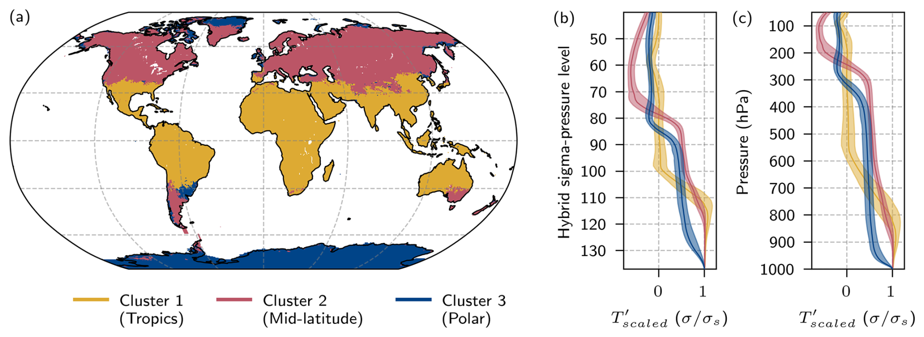
Figure 2 (a) Global distribution of the three area-weighted clusters over land: cluster 1 (yellow, N = 26 325 grid points), cluster 2 (red, N = 30 138), and cluster 3 (blue, N = 31 626). (b, c) median and interquartile range of the median vertical $T_{\mathrm{scaled}}^{\prime }$ profiles of all grid points in each cluster, (b) on sigma-hybrid model levels and (c) on pressure levels (surface pressure set to the reference pressure 1000 hPa).

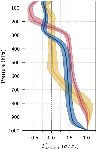
In the tropical cluster, we find that the positive temperature anomalies are confined to the near-surface and lower troposphere, with the highest temperature anomalies at about 900 hPa. In contrast, the mid- and upper-troposphere do not exhibit any temperature anomaly. The maximum boundary layer height, based on the Richardson number criterion (ECMWF, 2016), varies in these regions on days with TXx events roughly between 700 and 500 hPa (Fig. A1a). Since our temperature anomaly within the tropics is confined to about 600 hPa, this indicates that the temperature anomalies are restricted to the PBL. Note that not all tropical regions feature such deep PBLs, which are most frequent in arid subtropical regions (Fig. A1a). Due to variations of the PBL height, the interquartile range of $T_{\mathrm{scaled}}^{\prime }$ between model levels 100 and 120 is larger in the tropical compared to the other clusters (Fig. 2b). However, the fact that across the tropics, TXx temperature profiles have no anomaly in the free troposphere leads to the tropical and subtropical regions being clustered together. The absence of an upper-level temperature anomaly is consistent with the weak horizontal temperature gradient in the tropical free troposphere. This gradient is typically weak since gravity waves efficiently adjust the free-tropospheric temperature profile to a moist adiabatic profile throughout the tropics (Sobel and Bretherton, 2000; Nicholls et al., 1991; Holloway and Neelin, 2007). Recent research on tropical heat extremes suggested that they occur during periods of suppressed moist convection, caused either by reduced near-surface moisture (Byrne, 2021; Costa et al., 2022) or the entrainment of dry air (Duan et al., 2024). This suppression allows for the development of a deep PBL through dry convection within the PBL, facilitating the accumulation of heat and resulting in the high temperature anomalies observed in this cluster's distinct vertical profile.

Similar to the tropical cluster, the mid-latitude cluster features a deep layer of uniform and extremely high temperature anomalies near the surface (Fig. 2b, c). However, in contrast to the tropical cluster, it exhibits vertically deep temperature anomalies that extend throughout the troposphere. The temperature anomaly profile is bottom-heavy, with the largest temperature anomalies in terms of $T_{\mathrm{scaled}}^{\prime }$ and T^′ near the surface and in the lower troposphere since the standard deviation decreases from the surface to the free troposphere (Fig. C1). The same structure with the largest anomalies near the surface but still vertically deep anomalies was also noted by Noyelle et al. (2025) during extreme summers, Hotz et al. (2024) during recent record-shattering heatwaves, and Lhotka and Kyselý (2024) during European heat extremes. The presence of these deep temperature anomalies suggests that heat extremes in the mid-latitudes are more vertically organised than those over the tropics, likely due to dynamical coupling with the upper-level anticyclonic flow. Aside from the vertically organised behaviour of the mid-latitude cluster, it is particularly striking that, despite well-documented regional differences in the relative importance of different processes for the formation of mid-latitude heatwaves (e.g. Miralles et al., 2014; Zschenderlein et al., 2019; Röthlisberger and Papritz, 2023; Hotz et al., 2024), the vertical profiles in all these regions ultimately end up in the same mid-latitude cluster, underscoring their commonality in terms of vertical structure compared to other climate zones.

For the polar cluster, we also find temperature anomalies that extend throughout the troposphere, similar to the mid-latitude cluster (Fig. 2b, c). However, the layer near the surface with extremely high $T_{\mathrm{scaled}}^{\prime }$ is much thinner at high latitudes. As discussed in the introduction, climatologically, polar regions feature strong temperature inversions over the cold surface, leading to thin stable boundary layers with relatively small temperature variability (see Figs. A1b and C1). Therefore, the large near-surface temperature anomalies in the TXx profiles could hint at the erosion of this inversion layer and the mixing down of warmer air during heat extremes. This finding aligns with Blanchard‐Wrigglesworth et al. (2023) and Wille et al. (2024), who showed the erosion of the near-surface temperature inversion during the 2022 Antarctica heatwave. The mid- and upper-tropospheric normalised temperature anomalies are relatively weak compared to the near-surface anomalies. Given the large temperature anomalies near the surface, scaling with $T_{\mathrm{norm}}^{\prime }(k=\mathrm{0})$ scales the full profile more drastically, leading to lower normalised values in the free-troposphere compared to the mid-latitude cluster.

In the upper troposphere and lower stratosphere, profiles of the polar and in particular the mid-latitude clusters feature negative ${\stackrel{\mathrm{‾}}{T^{\prime }}}_{\mathrm{scaled}}$ above 250–300 hPa. These negative values are most likely due to the upward shift of the tropopause, associated with the upper-level anticyclones during heat extremes (e.g. Pfahl and Wernli, 2012). Therefore, virtually all positive temperature anomalies during TXx events are confined to the troposphere, and the negative anomalies above emerge as a consequence of the elevated tropopause. Weaker negative temperature anomalies for the polar cluster likely arise from weaker anticyclonic flow anomalies. The tropics also feature a small negative temperature anomaly around the tropopause height, consistent with the cooling of the lower stratosphere in response to tropospheric warming (Holloway and Neelin, 2007; Lin and Emanuel, 2024).

With our procedure, some regions are classified in somewhat unexpected clusters. For instance, in Europe, both the Iberian Peninsula and the west coast of France stand out as being assigned to the tropical cluster rather than the mid-latitude cluster (Fig. 2a). TXx events over the Iberian Peninsula feature a deep PBL and a vertically uniform layer of elevated scaled temperatures extending from the surface to 700 hPa (Fig. D1c, d). At the same time, there is also an upper-level temperature anomaly near the tropopause, similar to the mid-latitude cluster, even though this temperature anomaly is weaker and confined to the upper troposphere. While heat extremes in mid-latitude regions are typically linked to atmospheric blocking, over the Iberian Peninsula, they are more often associated with subtropical ridges (e.g. Pfahl and Wernli, 2012; Zschenderlein et al., 2019; Sousa et al., 2021). In addition, Sousa et al. (2019) and Cos et al. (2025) reported that heat extremes over the Iberian Peninsula are frequently accompanied by Saharan plumes of warm air in the free troposphere. Therefore, TXx events in this region feature a hybrid structure, combining characteristics of both the tropical and mid-latitude clusters. Another unexpected classification occurs in Greenland (Fig. 2a). Despite its snow cover, cold near-surface conditions, and a shallow PBL, TXx events over a large part of Greenland are classified as being in the mid-latitude rather than the polar cluster. Examining individual grid points over Greenland (Fig. D2b–e) reveals that the mid-latitude classified grid points feature a weaker vertical gradient of the temperature anomalies near the surface compared to those in the polar cluster. However, the near-surface layer with uniform temperature anomalies at the Greenland grid points classified as mid-latitude is shallow compared to the median of the mid-latitude cluster. Nevertheless, the temperature anomalies in the free troposphere are higher, similarly to the mid-latitude cluster, which likely leads to the mid-latitude classification. A third unexpected classification arises in South America, where parts of Uruguay and southern Brazil are in the polar cluster (Fig. 2a). Comparing the cluster median profile and the profiles at the considered grid points reveals that even though the temperature anomalies in the PBL deviate considerably from the polar cluster, the free-tropospheric temperature anomalies are similar to the polar cluster and, thus, smaller than in the mid-latitude cluster (Fig. D3d). The different characteristics of this region likely come from the different seasonality of the TXx events compared to the monsoon region further north (see Fig. S1) and the reduced co-location of upper-level blocking anticyclones during these events compared to the region further south (Rodrigues and Woollings, 2017; Gelbrecht et al., 2021). Note that, aside from unexpected clusters in these regions, elevated regions generally cluster with their “expected cluster”, indicating that topography itself does not affect the clustering (Figs. 2a and D2). Generally, we expect some grid points to feature a mix of characteristics of the three clusters, especially at the intersection between two clusters. Despite its caveats (e.g. due to the limitation to three clusters only), the clustering provides a coherent and informative overall picture of the vertical temperature anomaly structure. We will further discuss the spatial variability within the clusters (and therefore, the robustness of the cluster profiles) together with the variability of individual TXx events in Sect. 4.

Given that the extent of the troposphere varies meridionally, one might wonder whether the identified clusters simply reflect this variation in tropopause height. We therefore performed three sensitivity tests: (i) without an area-weighting of the grid points, (ii) with an area-weighting but with profiles that are capped in the mid-troposphere by only including the lowermost hybrid sigma–pressure levels (levels 90–137), and (iii) without an area-weighting where the profiles are vertically scaled and capped at the tropopause by linear scaling between the surface and the dynamical tropopause. The first test reveals a similar peak of the silhouette score (Fig. S2a), while the second shows a peak at four to five clusters, and the third one shows no peak and generally lower silhouette scores (Fig. S2b, c). The approaches produced very similar global distributions of the clusters and median cluster profiles when constraining the number of clusters to three, except for the second test, which features no polar but two tropical clusters (Fig. S3). We conclude from these tests that the clusters are not an artefact of varying tropopause height, but instead they capture differences in vertical temperature anomaly profiles that reveal distinct dynamics leading to the formation of heat extremes.

3.2 Genesis and decay of TXx events

To better understand the temporal evolution of the vertical structure of TXx events, we next examine the genesis and decay of temperature anomalies in the days preceding and following the events, respectively (Fig. 3). Even though the mechanisms forming near-surface heat extremes in the three clusters vary considerably, all three clusters experience an increase in the temperature anomaly within 5 d before the TXx event from an approximately climatological profile (close to zero anomalies at most levels) to the previously discussed profiles on the day of the TXx events (Fig. 3a–c).

Figure 3 Temporal evolution of the median and interquartile range of the median scaled temperature anomalies ($T_{\mathrm{scaled},C}^{\prime }$) of all the grid points (a–c) during the 5 d genesis and (d–f) 3 d decay of TXx events for (a, d) the polar, (b, e) mid-latitude, and (c, f) tropical clusters. The surface pressure is set again to a reference pressure of 1000 hPa.

Heat extremes in the tropics are characterised by a gradual and uniform increase in the temperature anomaly below 600 hPa (Fig. 3c). This suggests a local heat accumulation within the boundary layer, likely due to reduced soil and PBL moisture (Byrne, 2021; Costa et al., 2022; Duan et al., 2024). Mirroring the genesis phase, the decay of heat extremes in the tropics is characterised by a gradual decrease in the temperature anomaly within the PBL (Fig. 3f).

In contrast, the genesis of heat extremes in the mid-latitudes is characterised by a full tropospheric warming (Fig. 3b). In the period from 5 to 1 d before the TXx event, the scaled temperature anomaly increases uniformly throughout the troposphere. This vertically deep warming likely indicates an influence of large-scale atmospheric dynamics that preconditions the vertical profile before reaching the peak surface temperatures. One day before the TXx event, the temperature in the mid- to upper-troposphere nearly reached its final temperature anomaly, while the surface temperature anomaly still deviates strongly from the one during the TXx event. This suggests that the final warming occurs predominantly in the lower troposphere and PBL, presumingly due to land–atmosphere feedbacks, but potentially also due to amplified subsidence, as noted by Hotz et al. (2024) for the 2021 PNW heatwave. The evolution of temperature anomalies aligns with the evolution of recent heatwaves in the mid-latitudes, which also featured first a full tropospheric warming followed by a low-level intensification (Neal et al., 2022; Hotz et al., 2024; Lhotka and Kyselý, 2024).

After TXx events in the mid-latitudes, a strong decrease in temperature anomaly is observed first within the PBL, while the temperature anomalies above 800 hPa decrease more slowly (Fig. 3e). Note that the TXx event is the hottest time step by definition. Therefore, we expect a decrease in the near-surface temperature afterwards. However, principally anomalous temperatures can remain after a TXx event. Sauter et al. (2023) found that thunderstorms and frontal passages terminate heat extremes in central Europe, which aligns with the occurrence of precipitation after TXx events and their termination through moist convection, suggested by Zhang and Boos (2023). Aside from the specific termination processes, the longer-lasting temperature anomalies in the upper levels might also represent the different lifetimes of upper-level anticyclones and heat extremes.

Similar to the mid-latitudes, heat extremes in the polar cluster exhibit first a uniform warming throughout the troposphere (Fig. 3a). The difference in the vertical profile compared to the mid-latitude cluster emerges about 1 d before TXx events, when the temperature anomaly in the lowermost 50 hPa increases very strongly. Röthlisberger and Papritz (2023) found a strong advective contribution to near-surface temperature anomalies during heat extremes in polar regions. Furthermore, according to Hermann et al. (2020), a strong upper-tropospheric ridge and the associated poleward transport of warm and moist air masses are responsible for extreme melting events in Greenland. Therefore, we hypothesise that the deep temperature anomaly profiles that we observe in the polar cluster likely originate from strong advection. Aside from the deep temperature anomalies, the near-surface evolution of ${\stackrel{\mathrm{‾}}{T^{\prime }}}_{\mathrm{scaled}}$, as already discussed before, hints towards the rapid erosion of the above-ground temperature inversion layer. The intrusion of warm and moist air above the inversion can lead to its erosion through changes in the surface energy balance, rather than increased shear-driven turbulent mixing within the inversion layer (Wille et al., 2024). This erosion of the surface temperature inversion during our TXx events in the polar cluster is likely similar to observed, recent polar heatwaves. During the days after polar TXx events, the near-surface temperature anomalies continuously fade away. In contrast, the upper-level temperature anomaly decreases more slowly (Fig. 3d). Both suggest the restoration of a near-surface temperature inversion after a TXx event, which was also observed after the East Antarctica heatwave in 2022 (Wille et al., 2024).

3.3 Refinement of classification

Up to this point, our analysis focused on a k-means clustering with three clusters, which is the number of clusters for which the ratio of the within-cluster similarity and the between-cluster dissimilarity is the largest. As a refinement, we extend the analysis to six clusters. This choice is motivated by the consideration that by doubling the number of clusters, we can examine whether each of the three original clusters is partitioned into two sub-clusters, or whether qualitatively new groupings emerge.

The six resulting clusters from the area-weighted k-means clustering show, similarly to the three clusters, the major climate zones (compare Figs. 2a and 4a). Compared to the original clustering with three clusters, the refined clustering results in two clusters with tropical characteristics, three with mid-latitude characteristics, and one with polar characteristics. Hereafter, we focus on the different climate characteristics separately.

Figure 4 Refinement of the global area-weighted clustering with now six clusters over land: (a) map of clusters polar 1 (dark blue, N = 30 127 grid points), mid-latitude 1 (red, N = 9124), mid-latitude 2 (dark pink, N = 10 312), mid-latitude 3 (light pink, N = 17 422), tropics 1 (brown, N = 11 299), and tropics 2 (yellow, N = 9865). (b–d) Median and interquartile range of the vertical median scaled T^′ profile of all the grid points within each cluster for the (b) polar, (c) mid-latitude, and (d) tropical clusters on pressure levels (surface pressure set again to the reference pressure 1000 hPa).

In the tropical regions (Fig. 4d), we find a distinction between regions with deeper PBLs with positive T^′ (tropics 2) and regions with a less deep layer with positive T^′ (tropics 1), while the profiles look similar above 500 hPa (no anomalies in both clusters). Comparing these clusters to the soil moisture regimes of Schwingshackl et al. (2017), we find that the regions with the shallower PBL are often situated in regions classified in a wet or transitional-wet regime, whereas the tropics 2 cluster is located in regions classified in the dry or transitional regime, especially over deserts, i.e. below the descending branch of the Hadley cell. In dry regions, the sensible heat fluxes are stronger than in wet regions, as a larger fraction of the net radiation is converted into sensible heat flux (e.g. Seneviratne et al., 2010). This larger heat transfer into the atmosphere leads to a deeper PBL (Miralles et al., 2014; Santanello et al., 2007).

All mid-latitude clusters feature deep temperature anomalies (Fig. 4c), but the mid-latitude 1 cluster has a stronger vertical decrease of ${\stackrel{\mathrm{‾}}{T^{\prime }}}_{\mathrm{scaled}}$, while clusters mid-latitude 2 and 3 exhibit a more vertically uniform anomaly profile. The layer of high temperature anomalies near the surface is shallower in mid-latitude 3 compared to mid-latitude 2. The stronger vertical gradient in ${\stackrel{\mathrm{‾}}{T^{\prime }}}_{\mathrm{scaled}}$ between 800 and 600 hPa in the mid-latitude 1 cluster indicates that its temperature anomalies are more concentrated near the surface. Furthermore, the deeper uniform layer of ${\stackrel{\mathrm{‾}}{T^{\prime }}}_{\mathrm{scaled}}$ in this cluster near the surface suggests a deeper PBL and suggests that surface processes may be more important. In contrast, the stronger upper-tropospheric anomalies in cluster mid-latitude 2 and mid-latitude 3 are likely linked to stronger anticyclones or atmospheric blocks, as also indicated by a strong negative anomaly above the tropopause. Lhotka and Kyselý (2024) also differentiated European heat extremes by their vertical temperature distribution and noted that heat extremes with amplified temperature anomalies near the surface were often preconditioned by low soil moisture. Furthermore, according to Schwingshackl et al. (2017), large parts of the mid-latitude 1 cluster regions are located in the transition soil moisture regime, while the mid-latitude 2 and mid-latitude 3 cluster regions are in the wet regime. Connecting this knowledge with our clusters, the mid-latitude 1 cluster, with its deeper PBL, has likely stronger sensible heat fluxes and, thus, a stronger land-atmosphere coupling due to drier soil moisture conditions.

Considerable changes occur in climatic transition zones between the original three-cluster and the extended six-cluster categorisation. In these regions, some grid points change their cluster type. For example, the Iberian Peninsula, which was initially part of the tropical cluster, has now shifted to the mid-latitude 1 cluster with weak temperature anomalies in the upper troposphere and deep PBL anomalies, which fits better with the observed $T_{\mathrm{scaled}}^{\prime }$ of that region (see grey shading in Fig. D1c, d). Similarly, the South American regions, which were assigned to the polar cluster due to their weak upper-level temperature anomalies, are now classified as mid-latitude 1.

The polar cluster is similar to the polar cluster of the original clustering (Figs. 2a and 4a). Having only one polar cluster in the refined clustering suggests that the variability between polar grid points is comparatively small due to the shallow near-surface layer with high temperature anomalies.

In the remaining parts of the paper, we return to the analysis of the original classification with three clusters.

4 Inter-cluster variability and the variance of individual TXx events

As detailed in Sect. 2.4, we partition the mean squared error (MSE) between individual TXx profiles and the cluster median profile at each grid point into contributions of a bias and a variance (see Eq. 9). The former, the grid point's ${\mathrm{bias}}^{\mathrm{2}}\left({\stackrel{\mathrm{‾}}{T^{\prime }}}_{\mathrm{scaled}}\right)$, represents the squared bias between the median vertical profile (${\stackrel{\mathrm{‾}}{T^{\prime }}}_{\mathrm{scaled}}$) and cluster median, while the latter, $\mathrm{var}\left(T_{\mathrm{scaled}}^{\prime }\right)$, captures the variance between individual TXx profiles and the median ${\stackrel{\mathrm{‾}}{T^{\prime }}}_{\mathrm{scaled}}$ at a particular grid point. Large values of ${\mathrm{bias}}^{\mathrm{2}}\left({\stackrel{\mathrm{‾}}{T^{\prime }}}_{\mathrm{scaled}}\right)$ mean that the $T_{\mathrm{scaled}}^{\prime }$ profiles differ greatly from the cluster median, while large values of $\mathrm{var}\left(T_{\mathrm{scaled}}^{\prime }\right)$ indicate that the $T_{\mathrm{scaled}}^{\prime }$ profiles at a single grid point are highly variable between TXx events. In the following, we consider ${\mathrm{bias}}^{\mathrm{2}}\left({\stackrel{\mathrm{‾}}{T^{\prime }}}_{\mathrm{scaled}}\right)$ and $\mathrm{var}\left(T_{\mathrm{scaled}}^{\prime }\right)$ separately (Fig. 5).

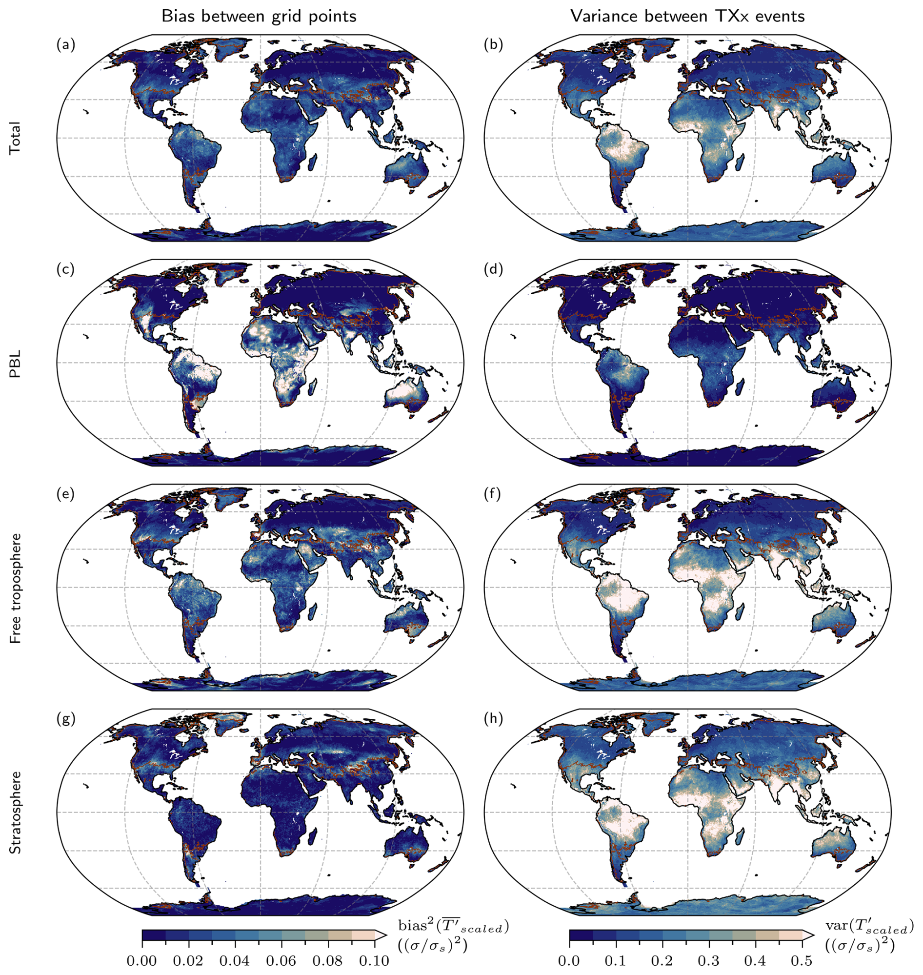
Figure 5 Distribution of (left) ${\mathrm{bias}}^{\mathrm{2}}\left({\stackrel{\mathrm{‾}}{T^{\prime }}}_{\mathrm{scaled}}\right)$ and (right) $\mathrm{var}\left(T_{\mathrm{scaled}}^{\prime }\right)$, vertically averaged over (a, b) all hybrid sigma–pressure levels, (c, d) only the PBL, (e, f) only the free troposphere, and (g, h) only the stratosphere. The brown lines denote the boundaries between the three clusters. The coldest 10 TXx events are excluded at each grid point. Note the different scales used for ${\mathrm{bias}}^{\mathrm{2}}\left({\stackrel{\mathrm{‾}}{T^{\prime }}}_{\mathrm{scaled}}\right)$ and $\mathrm{var}\left(T_{\mathrm{scaled}}^{\prime }\right)$.

Generally, ${\mathrm{bias}}^{\mathrm{2}}\left({\stackrel{\mathrm{‾}}{T^{\prime }}}_{\mathrm{scaled}}\right)$ is relatively small and uniform within the clusters, except for the tropics (Fig. 5a). This highlights that our clustering is generally working adequately. However, we want to highlight some regions in the following. As already exemplarily explained for Spain in Sect. 3.1, profiles can exhibit mixed characteristics of two clusters in regions where the vertical extent of the temperature anomalies is more variable. Therefore, along the border between clusters, we expect and also find elevated values of ${\mathrm{bias}}^{\mathrm{2}}\left({\stackrel{\mathrm{‾}}{T^{\prime }}}_{\mathrm{scaled}}\right)$ (Fig. 5a). Introducing more clusters, as in Sect. 3.3, reduces ${\mathrm{bias}}^{\mathrm{2}}\left({\stackrel{\mathrm{‾}}{T^{\prime }}}_{\mathrm{scaled}}\right)$ considerably in these regions (Fig. S5). Furthermore, parts of Greenland, Uruguay, and Brazil feature high ${\mathrm{bias}}^{\mathrm{2}}\left({\stackrel{\mathrm{‾}}{T^{\prime }}}_{\mathrm{scaled}}\right)$. Considering contributions from different vertical layers to the bias, we find that all regions feature relatively high biases in the PBL (Fig. 5c) and low biases in the free troposphere and stratosphere (Fig. 5e, g). As already discussed in Sect. 3.1, these regions feature similar temperature anomalies in the upper troposphere, while the near-surface temperature anomaly profiles deviate from the cluster median (Figs. D2 and D3). Other regions with high ${\mathrm{bias}}^{\mathrm{2}}\left({\stackrel{\mathrm{‾}}{T^{\prime }}}_{\mathrm{scaled}}\right)$ are in the tropical cluster. Considering the different layers (Fig. 5c, e, g) reveals that the largest values of ${\mathrm{bias}}^{\mathrm{2}}\left({\stackrel{\mathrm{‾}}{T^{\prime }}}_{\mathrm{scaled}}\right)$ are located in the PBL. This is consistent with the fact that with six clusters we find two tropical clusters with a shallow and deep PBL, respectively, and then ${\mathrm{bias}}^{\mathrm{2}}\left({\stackrel{\mathrm{‾}}{T^{\prime }}}_{\mathrm{scaled}}\right)$ reduces considerably (Figs. A1 and S5). Therefore, elevated values of ${\mathrm{bias}}^{\mathrm{2}}\left({\stackrel{\mathrm{‾}}{T^{\prime }}}_{\mathrm{scaled}}\right)$ in the tropical cluster originate from the different vertical extent of the PBL.

Considering now the variability between TXx events at each grid point ($\mathrm{var}\left(T_{\mathrm{scaled}}^{\prime }\right)$), we first note that this quantity is a factor five larger than the bias ${\mathrm{bias}}^{\mathrm{2}}\left({\stackrel{\mathrm{‾}}{T^{\prime }}}_{\mathrm{scaled}}\right)$ (Fig. 5a, b, note the different scales). Therefore, variability in the vertical profiles within each cluster is mainly dominated by differences between events rather than by differences in the median profiles between grid points. Second, the global distribution of $\mathrm{var}\left(T_{\mathrm{scaled}}^{\prime }\right)$ shows a clear meridional pattern (Fig. 5b). We find large values in the tropics, which decrease towards a minimum in the mid-latitudes and increase again towards the poles. This implies that, when considering variability in the entire vertical column, mid-latitude TXx events are more alike in terms of their scaled temperature anomaly profiles than events in the tropics and polar regions. In the following, we focus on each of the three climate zones separately.

In the tropics, the anomalous temperatures are confined to the PBL, where the variance is relatively low, while the free-tropospheric profile is basically unconstrained (Fig. 5d, f). Therefore, if the tropical region features a heat extreme, its relevant part of the vertical profile looks much like the profile of other heat extremes, as the $\mathrm{var}\left(T_{\mathrm{scaled}}^{\prime }\right)$ within the PBL is small. However, to have a precise description of the vertical profile, the climatological PBL height is needed due to the large ${\mathrm{bias}}^{\mathrm{2}}\left({\stackrel{\mathrm{‾}}{T^{\prime }}}_{\mathrm{scaled}}\right)$. Therefore, the large variability of the entire profiles in the tropics seen in Fig. 5b stems from the vertical layers above the PBL that are not relevant for the formation of the TXx event.

Moving to the mid-latitudes, the $\mathrm{var}\left(T_{\mathrm{scaled}}^{\prime }\right)$ declines (Fig. 5b). Here, TXx events have vertically deep temperature anomalies, extending up to the tropopause. Therefore, the lower $\mathrm{var}\left(T_{\mathrm{scaled}}^{\prime }\right)$, in general and in the free troposphere, together with these deep temperature anomalies, highlights that the near-surface temperatures are strongly coupled to the temperature anomaly over the whole troposphere, underlining the interplay between large-scale dynamics and near-surface processes in shaping heat extremes in the mid-latitudes (Fig. 5f). Both ${\mathrm{bias}}^{\mathrm{2}}\left({\stackrel{\mathrm{‾}}{T^{\prime }}}_{\mathrm{scaled}}\right)$ and $\mathrm{var}\left(T_{\mathrm{scaled}}^{\prime }\right)$ are small in the mid-latitudes (Fig. 5a, b). Therefore, the cluster median provides a good representation of individual profiles.

Even though the polar regions also feature vertically deep temperature anomalies up to the tropopause, $\mathrm{var}\left(T_{\mathrm{scaled}}^{\prime }\right)$ increases again (Fig. 5b). Here, near-surface temperature inversions strongly modulate the vertical profile of $T_{\mathrm{scaled}}^{\prime }$. Depending on how strong the erosion of the temperature inversion is, the vertical structure changes considerably, leading to higher $\mathrm{var}\left(T_{\mathrm{scaled}}^{\prime }\right)$. Together with the climatological strength of the near-surface temperature inversion layer, whose erosion creates high $\mathrm{var}\left(T_{\mathrm{scaled}}^{\prime }\right)$, the profiles in polar regions are more variable and, thus, less constrained than in other regions.

5 Vertical temperature anomaly structure of the most intense events

So far, we have classified heat extremes based on their vertical structure and analysed the variability between regions and individual TXx events. As detailed in the introduction, it has been suggested that the vertical temperature structure could be a key for explaining the, in cases record-shattering, intensity of recent surface heat extremes (e.g. Neal et al., 2022; Zhang and Boos, 2023). Therefore, we now investigate the warmest 10 TXx events at each grid point (Fig. 6) to see whether their profiles deviate from the median of all TXx events ($\mathrm{var}\left(T_{\mathrm{scaled}}^{\prime }\right)$).

Figure 6 (a) Variance of $T_{\mathrm{scaled}}^{\prime }$ profiles for the 10 hottest TXx events relative to the median profile of all TXx events ($\mathrm{var}\left(T_{\mathrm{scaled}}^{\prime }\right)$), and (b) the ratio of $\mathrm{var}\left(T_{\mathrm{scaled}}^{\prime }\right)$ between the hottest 10 TXx events and moderate TXx events (which exclude the hottest and coldest 10 TXx events). Fields in both panels are vertically averaged over all hybrid sigma–pressure levels. The brown lines denote the boundaries between the three clusters.

Overall, the spatial distribution of $\mathrm{var}\left(T_{\mathrm{scaled}}^{\prime }\right)$ of the most intense TXx events across the globe is similar compared to all TXx events (Fig. 6a). As discussed in the previous section, $\mathrm{var}\left(T_{\mathrm{scaled}}^{\prime }\right)$ shows a meridional pattern of high values in the tropics, a local minimum in the mid-latitudes, and slightly higher values in the polar regions.

Considering the $\mathrm{var}\left(T_{\mathrm{scaled}}^{\prime }\right)$ ratio between the hottest and the more moderate TXx events (excluding the top and bottom 10 TXx events), this ratio is < 1 virtually all across the globe, meaning that the variance for the hottest events is lower than for the moderate events (Fig. 6b). This implies that the most extreme TXx events are less variable from one event to another and more alike the cluster median than moderate TXx events.

Figure 7 Joint distributions of the mean vertical variance of individual TXx event profiles relative to their median profile and near-surface $T_{\mathrm{scaled}}^{\prime }(k=\mathrm{0})$ (lowest model level), (a) for $T_{\mathrm{norm}}^{\prime }$, (b) $T_{\mathrm{scaled}}^{\prime }$, and (c) $T_{\mathrm{scaled}}^{\prime }$ in log-log-scale. The values of ρ in the upper right corner in panels (a) and (b) denote the Spearman correlation (both p-values $<{\mathrm{10}}^{-\mathrm{3}}$). Bin widths are 0.1σ (x-axis) and 0.02σ or 0.02$\mathit{\sigma }/{\mathit{\sigma }}_{\mathrm{s}}$ (y-axis). The black dotted line marks the weighted median. The violet dotted line and the m value in the upper right corner in panel (c) indicate the regression line and slope, respectively. Note that the negative $T_{\mathrm{scaled}}^{\prime }(k=\mathrm{0})$ values on the x-axes arise from our event definition and make up 0.03 % of the TXx events.

The most intense TXx events represent the far tail of the temperature anomaly distribution. This has important implications for interpreting vertical profiles of $T_{\mathrm{norm}}^{\prime }$ and $T_{\mathrm{scaled}}^{\prime }$. Specifically, $T_{\mathrm{norm}}^{\prime }$ shows a nearly constant variance in observed TXx events across different intensities (Fig. 7a). In contrast, the variance of $T_{\mathrm{scaled}}^{\prime }$ TXx profiles decreases with increasing intensity (Fig. 7b). The decrease is proportional to $\mathrm{1}/{\mathit{\sigma }}^{\mathrm{2}}$, visible in the linear relationship with a slope of −2 in the log-log plot (Fig. 7c). This means that more intense heat extremes have a similar absolute deviation from their normalised temperature anomaly profiles but a smaller relative deviation from the cluster median. For example, both a 2σ-event and a 4σ-event have an error of roughly 0.5σ in the normalized temperature anomalies. However, the relative error for the 4σ-event is actually four times as low as for the 2σ-event. In this sense, as events become more extreme, their vertical structure becomes more typical.

This emergence of “typicality” aligns with the predictions of large deviation theory (LDT), a mathematical framework that provides insights into the statistics and dynamics of such rare events (e.g. Gálfi et al., 2021; Lucarini et al., 2023; Noyelle et al., 2024). Within the LDT, the principle of “typicality” states that highly improbable events occur through the most probable pathway (Touchette, 2009). Physically, even though an event is extremely rare, it forms through similar processes as more likely events and is therefore not an outlier in terms of its dynamics. Lucarini et al. (2023) demonstrated dynamical typicality for the Northwest Pacific 2021 heatwave in long simulations with an Earth system model, and Noyelle et al. (2024) found converging physical mechanisms leading to increasingly extreme temperatures in a 2000-year climate model simulation. Our clustering analysis extends previous findings with long model simulations to reanalysis data, showing that a typicality of vertical temperature profiles emerges as events become more extreme. This provides observational support for LDT predictions and reinforces the idea that the most extreme heatwaves emerge from increasingly constrained dynamical pathways.

Taken together, these results demonstrate that while moderate TXx events still exhibit a degree of diverse vertical structures, the most extreme heat events increasingly converge to a “typical” profile that is well captured by the cluster medians. Furthermore, it suggests that we can predict how the vertical profile of the very extreme events will be shaped with low relative error. This convergence towards a “typical” profile means that the most extreme TXx events are actually no freak events, despite their rarity.

6 Conclusions

Motivated by recent work on the vertical structure of heat extremes (Neal et al., 2022; Hotz et al., 2024; Lhotka and Kyselý, 2024), we present an Eulerian global classification of the vertical temperature anomaly structure of TXx events over land using area-weighted k-means clustering. By first calculating temperature anomalies and then normalising them by the standard deviation, we accounted for regional climate variability. We then take the step of scaling each vertical temperature profile by its surface value, yielding a scaled temperature profile ($T_{\mathrm{scaled}}^{\prime }$). This allows us to compare the shape of a heat extreme's vertical structure independent of its local intensity or climate zone. This scaling procedure is essential, as it enables the subsequent application of a k-means clustering algorithm to these scaled profiles, identifying three distinct clusters, i.e., regional groups with similar vertical temperature anomaly characteristics.

We find, first, that the global distribution of the three clusters broadly follows climate zones, highlighting that while heat extremes can form through multiple pathways, they tend to converge onto a limited set of vertical $T_{\mathrm{scaled}}^{\prime }$ structures. In the tropics, temperature anomalies are mainly confined to the boundary layer, while in the mid-latitudes and polar regions, positive temperature anomalies extend throughout the troposphere. Polar regions feature only a shallow layer of amplified positive temperatures near the surface, whereas the mid-latitudes exhibit a deeper layer of strong positive temperature anomalies.

Second, the temporal evolution of these clusters in the days before and after TXx events indirectly highlights distinct physical mechanisms. In the tropics, heat extremes build up gradually through progressive boundary-layer warming and heat accumulation, reflecting strong coupling with the land surface, possibly through reduced moisture within the PBL, or entrainment of dry air aloft (Byrne, 2021; Costa et al., 2022; Duan et al., 2024). In contrast, TXx events in mid-latitudes are characterised by deep tropospheric warming, associated with an upper-level anticyclonic flow, followed by an intensification of low-level anomalies in the final days, which is consistent with increased subsidence and surface feedbacks (Miralles et al., 2014; Hotz et al., 2024). In polar regions, the temporal evolution reveals the erosion of near-surface temperature inversions prior to heat extremes (Wille et al., 2024). Once these inversion layers are weakened, strong warming signatures emerge close to the ground while the overlying tropospheric profile warmed prior to the erosion of the surface inversion.

Third, while the deviation between the grid points' median profile and the cluster profile is relatively small, we find larger variations when comparing individual TXx events to their grid point median. The variance between TXx events and the bias to the cluster profile is lowest in the mid-latitudes, indicating that the ground temperature is strongly coupled to the temperature in the mid and lower troposphere, and the mid-latitude cluster profile is a good approximation of the vertical temperature profile for individual events. The bias between grid points is larger in polar regions, likely due to the variable strength of surface temperature inversion layers, while the variance between individual TXx events is similar or slightly larger than in the mid-latitudes. Tropical regions feature the largest biases between the grid points due to different PBL heights, compared to the other clusters. The variance between individual TXx events at one grid point is relatively low in the layers relevant for tropical heat extremes.

Finally, a very important result of our analyses is that compared with moderate TXx events, profiles during the most intense TXx events tend to follow the median profiles more closely. This “typicality” of extremes supports theoretical expectations from large deviation theory, whereby increasingly intense events emerge from more constrained dynamical pathways. Whereas this behaviour was previously observed only in long simulations (e.g. Lucarini et al., 2023; Noyelle et al., 2024), our clustering-based resampling reveals a similar pattern in observation-based reanalysis data.

Our results are based on several choices regarding the selection of extreme heat events, the number of clusters, the clustering method, and the extent of the vertical profile for clustering. However, our sensitivity analyses have shown that our results are robust to changes in the input parameters. Since we aimed for a simple global classification, unavoidably, not all vertical profiles align perfectly with the actual temperature anomaly profile during heat extremes at every grid point, but a large fraction of heat extremes, in particular the strongest ones, are well represented. Furthermore, we chose to apply the clustering to the median profiles for each grid point. Therefore, our clustering reveals the characteristics of a climatological heat extreme at each grid point. An additional next step could be investigating extended (multi-day) heat waves instead of hourly TXx events or the classification of different types of TXx events at each grid point, similar to Lhotka and Kyselý (2024). Furthermore, this Eulerian view of the characteristics of TXx events opens new questions, like whether these temperature anomalies within the clusters arise from distinct processes despite being classified as belonging to the same cluster. Therefore, one could combine our results with a Lagrangian analysis, learning more about the processes around the globe that shape these vertical temperature anomaly profiles, as done by Röthlisberger and Papritz (2023) and Hotz et al. (2024).

Appendix A: PBL height during TXx events

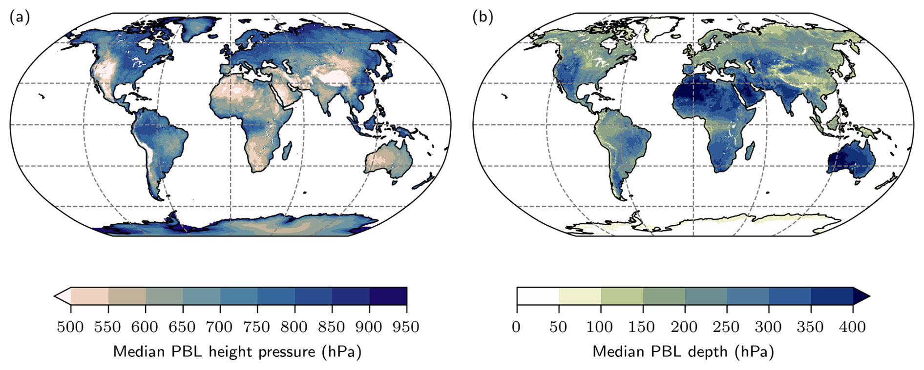
Figure A1 Global distribution of (a) the median PBL height (in hPa), and (b) the median PBL depth (also in hPa) during the 73 TXx events at each grid point.

Appendix B: Silhouette score of the area-weighted k-means clustering

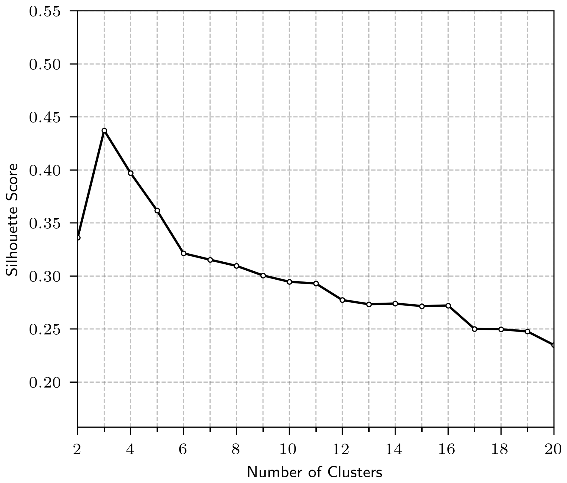
Figure B1 Silhouette score for finding an optimal number of clusters of the median scaled T^′ profiles over land grid points with the area-weighted k-means clustering approach, using the eight retaining components of all hybrid sigma-pressure levels.

Appendix C: Mean standard deviation of the temperature anomaly during TXx events

Figure C1 Global distribution of the mean standard deviation of the temperature anomaly at TXx events (a) at the lowest model level and the ratio of (b) interpolated to 700 hPa, (c) 500 hPa, and (d) 300 hPa to the lowest model level. The white areas over land in panel (b) are where the surface pressure is below 700 hPa.

Appendix D: Zoomed in maps of the k-means clustering with three clusters

Here we focus on Greenland, Europe, and South America and show regional excerpts of our global k-means clustering, weighted by latitude, with three clusters. Figures D1, D2, and D3 show, at selected grid points, how the vertical normalised temperature anomaly profile during TXx events compares to the corresponding median cluster profile. The figures help to put the results in Sect. 3.1 into context.

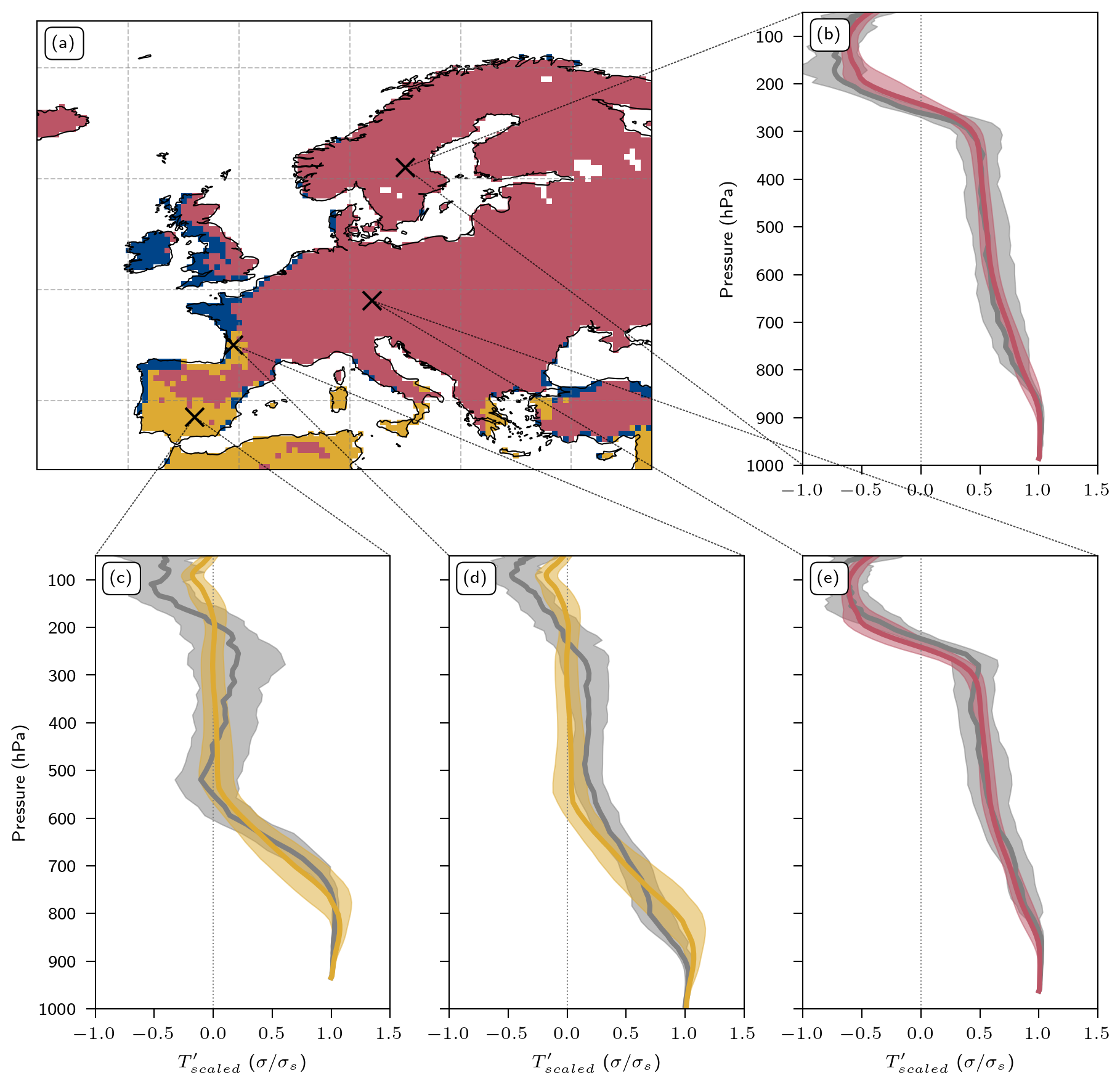
Figure D1 Area-weighted k-means clustering with three clusters from Fig. 2a shown as (a) a zoomed in map of Europe and (b–e) vertical $T_{\mathrm{scaled}}^{\prime }$ profiles for individual grid points at (b) 61° N, 15° E, (c) 38.5° N, 4° W, (d) 45° N, 0.5° W, and (e) 49° N, 12° E. The grey line and its shading denote the median and interquartile range of all TXx events at that grid point, the yellow, red, and blue lines and shading the clusters' median and interquartile range of all ${\stackrel{\mathrm{‾}}{T^{\prime }}}_{\mathrm{scaled}}$ within the tropical, mid-latitude, and polar clusters, respectively. For the cluster ${\stackrel{\mathrm{‾}}{T^{\prime }}}_{\mathrm{scaled}}$ profiles, we use the median surface pressure of the TXx events as a reference pressure to interpolate on pressure levels.

Figure D2 Area-weighted k-means clustering with three clusters from Fig. 2a shown as (a) a zoomed in map of Greenland and (b–e) vertical $T_{\mathrm{scaled}}^{\prime }$ profiles for individual grid points, (b) 70° N, 30° W, (c) 78° N, 61° W, (d) 64° N, 45° W, and (e) 78° N, 41° W. The grey line and its shading denote the median and interquartile range of all TXx events at that grid point, the red and blue lines and shading the clusters' median and interquartile range of all ${\stackrel{\mathrm{‾}}{T^{\prime }}}_{\mathrm{scaled}}$ within the mid-latitude and polar clusters, respectively. For the cluster ${\stackrel{\mathrm{‾}}{T^{\prime }}}_{\mathrm{scaled}}$ profiles, we use the median surface pressure of the TXx events as a reference pressure to interpolate on pressure levels.

Figure D3 Area-weighted k-means clustering with three clusters from Fig. 2a shown as (a) a zoomed in map of South America and (b–e) vertical $T_{\mathrm{scaled}}^{\prime }$ profiles for individual grid points, (b) 12° S, 45° W, (c) 46° S, 70° W, (d) 30° S, 60° W, and (e) 5° S, 65° W. The grey line and its shading denote the median and interquartile range of all TXx events at that grid point, the yellow, red, and blue lines and shading the clusters' median and interquartile range of all ${\stackrel{\mathrm{‾}}{T^{\prime }}}_{\mathrm{scaled}}$ within the tropical, mid-latitude, and polar clusters, respectively. For the cluster ${\stackrel{\mathrm{‾}}{T^{\prime }}}_{\mathrm{scaled}}$ profiles, we use the median surface pressure of the TXx events as a reference pressure to interpolate on pressure levels.