Building blocks of localized storm tracks: revisiting asymmetries between the NH and SH in storm track strength

An intermediate-complexity moist general circulation model is used to investigate the forcing of localized storm tracks by land–sea contrast, horizontal gradients in ocean heat uptake, planetary albedo, and topography. The additivity of the response to these building blocks is investigated. Consistent with previous work focusing on stationary waves, the storm track patterns and strength are not simply the linear additive sum of the response to each surface inhomogeneity. As observed on Earth, the SH storm tracks are stronger than those in the NH, and also stronger over ocean basins than over continents. In this model, the most important building block for this asymmetry is land–sea contrast, however, there is substantial non-additivity both in the regional structure and also the hemispheric asymmetry. An energy budget perspective offers some insight on the causes of the non-additivity, and highlights how the net impact of each building block on outgoing longwave radiation is dependent on the existence of the others. Relatively small changes in oceanic heat transport from the Southern Ocean to the North Atlantic have a pronounced impact on the individual terms making up the energy budget, however there is substantial cancellation between these terms leading to a small impact on the NH vs. SH asymmetry in storm track strength. The detailed structure of albedo has a weak impact on the NH vs. SH asymmetry due to substantial cancellation between the changes in individual terms making up the energy budget, even though the albedo profile has a large impact on the overall transient eddy activity in each hemisphere.

1 Introduction

The climate of the Earth is decidedly not zonally symmetric due to inhomogeneities in the lower boundary, such as the land-ocean distribution and orography. The land-ocean distribution directly impacts the distribution of surface temperature and moisture, while mountains directly impact the atmospheric flow (e.g., Held et al., 2002). These surface inhomogeneities both force stationary waves and perturb transient waves, organizing variability into localized storm tracks.

In the ERA5 reanalysis (Hersbach et al., 2020), storm activity is notably stronger in the North Atlantic and North Pacific sector in the NH, and in the Indian Ocean sector in the Southern Hemisphere (Fig. 1a; Inatsu and Hoskins, 2004). In the hemispheric mean, storm activity is also stronger in the Southern Hemisphere than in the Northern Hemisphere (Shaw et al., 2022). The goal of this paper is to understand how zonal inhomogeneities in the lower boundary lead both to this localization of storm tracks and to stronger SH storm activity. Our primary focus is on the annual average.

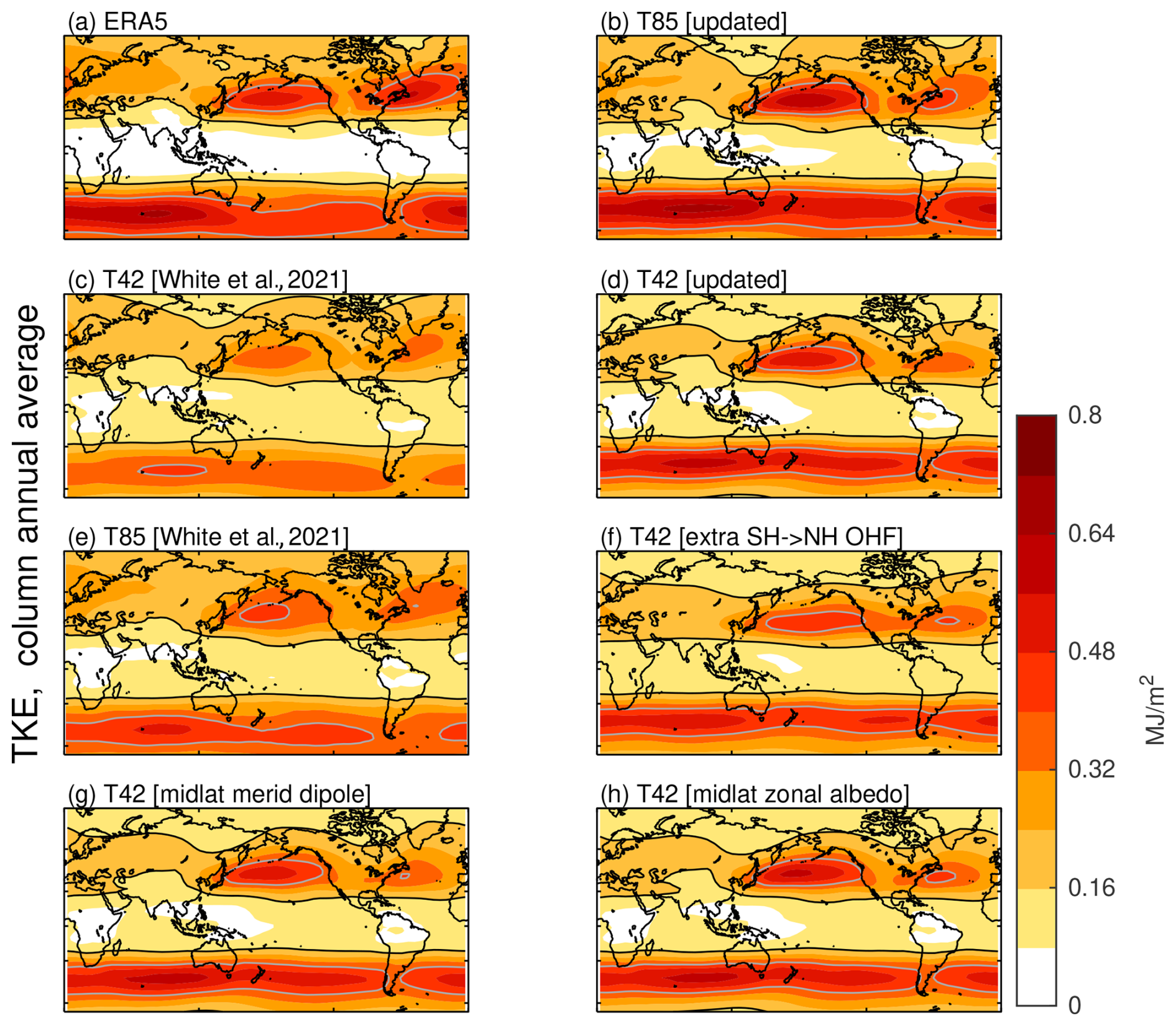
Figure 1 Column-integrated transient kinetic energy (2–8 d bandpass filtered; see Eq. 1 and Sect. 2.1 for methodological details), annual average, in ERA5 and in seven MiMA configurations with different resolutions and representations of albedo and ocean heat transport, but with all three of the surface inhomogeneities included: land–sea contrast, topography, and ocean heat transport. The configuration in panel (d) is denoted as ALL3 in all subsequent figures, and the hemispheric asymmetry in storm track strength for panels (b), (d), (f), (g), and (h) are shown in Fig. 11.

There are three primary surface zonal inhomogeneities of relevance to storm tracks. First, the land–ocean distribution can affect storm tracks via differences in land–sea heat capacity and subsequent surface temperature gradients, and also via variations in moisture availability and surface roughness (Brayshaw et al., 2009). Second, orography provides a localized drag on near-surface winds, and helps seed downstream storm tracks (Manabe and Terpstra, 1974; Pithan et al., 2016; Gerber and Vallis, 2009). Third, ocean-heat transport can set up zonal and meridional gradients in sea surface temperatures which can locally invigorate storm tracks (Brayshaw et al., 2011; Booth et al., 2012). In addition to these three surface inhomogeneities, albedo regulates temperature gradients and baroclinicity. All of these processes also affect planetary scale stationary eddies (Garfinkel et al., 2020c), which in turn will modify storm track structure.

Previous work has examined the effect of all of these surface inhomogeneities for storm track structure using two different classes of methodologies. First, several studies have introduced these inhomogeneities in an idealized manner onto a flat-bottomed aquaplanet general circulation model (Inatsu and Hoskins, 2004; Brayshaw et al., 2009, 2011; Saulière et al., 2012), but there was little attempt to globally reconstruct the observed storm tracks. A second approach is to begin with a comprehensive atmospheric general circulation model and omit particular features (typically just one or two of the three) from a complete, “realistic” set of lower boundary conditions, either with observed SSTs or a slab ocean with prescribed ocean heat uptake from observations (e.g., Manabe and Terpstra, 1974; Shaw et al., 2022), or coupled to a dynamic ocean model (e.g., Singh et al., 2016). A study that can fully bridge these two categories – aquaplanet to a realistic configuration – is currently lacking. While previous work has noted non-additivities when focusing on some of these inhomogeneities for regional storm tracks (e.g., Brayshaw et al., 2011), though not for SH vs. NH asymmetries (Shaw et al., 2022), a configuration that can allow for inclusion or removal of any of the three is needed in order to both characterize the nature of nonlinearities and nonadditivies that underlay storm tracks, and to fully evaluate the role of each of the three.

CMIP class models represent time-mean storm tracks well in the historical climate, including the SH vs. NH asymmetry (Donohoe et al., 2020) and the localization of storm tracks in specific basins (Priestley et al., 2020). Nonetheless, recent work has demonstrated that there are emerging discrepancies in storm track trends between CMIP models and observations in some regions (Kang et al., 2024a; Simpson et al., 2025), though not in others (Chemke and Coumou, 2024; Kang et al., 2024b), and also revealed lingering biases in both storm track strength and location (Priestley et al., 2023a, b). This motivates us to revisit the core question of why storm tracks are localized in the first place, and why they are stronger in the SH. Such a return to fundamentals might help us interpret why a CMIP class model struggles to simulate storm track trends in response to external forcings, and also focus on processes whose representation could be improved to help remove remaining biases.

We tackle these challenges using an intermediate complexity moist general circulation model (GCM) with full radiation coupled to a slab ocean with a steady ocean heat flux and thus implicit ocean heat transport (OHT). This GCM can be run both in aquaplanet mode, or with any combination of the three boundary inhomogeneities: land–sea contrast, OHT, and topography. The planetary albedo can also be specified to mimic either observations or the albedo from a comprehensive GCM. Furthermore, any arbitrary profile of ocean heat flux can be inserted in the slab ocean, and hence we can better understand how uncertainties in ocean heat transport affect atmospheric storm tracks. Any combination of these inhomogeneities can be imposed. While in a practical sense these inhomogeneities are coupled – it is difficult to imagine topography in a world without land, and ocean heat transport would be radically different in a world without continents – the intermediate complexity GCM allows for holding each of these three fixed at Earth-like settings independent of the rest (e.g., water mountains; Fig. 3 of Jucker and Gerber, 2017). This flexibility is the primary motivation for using a simpler model. A key simplication of the model is to not explicitly represent cloud radiative effects; instead, an albedo profile is imposed. Cloud radiative effects suffer from biases and large intermodel spread in CMIP models (Vignesh et al., 2020; Schuddeboom and McDonald, 2021; Jian et al., 2020; Medeiros et al., 2023), and given these uncertainties, arguably a better understanding of storm track asymmetries can be achieved by imposing a realistic albedo profile than by using a comprehensive GCM with biased shortwave fluxes.

We introduce the model setup, the experiments performed, and the diagnostics used in Sect. 2. After documenting the realism of the storm tracks in the intermediate complexity GCM in Sect. 3, we discuss the zonal structure of storm tracks in Sect. 4 and the SH vs. NH asymmetry in storm tracks in Sect. 5. Sensitivity tests to the details of the specification for albedo and ocean heat transport are shown in Sect. 6. A discussion and summary are presented in Sect. 7.

2 Methods

2.1 Model of an idealized Moist Atmosphere (MiMA)

To fully isolate and understand the statistical properties of storm tracks, it is necessary to systematically add or subtract key processes to a nonlinear moist GCM (Hoskins, 1983), due to the pronounced role of latent heat release in storm track structure (Shaw et al., 2018; Shaw and Graham, 2020; Schemm, 2023; Auestad et al., 2025). In this study, we use the Model of an idealized Moist Atmosphere (MiMA), developed by Jucker and Gerber (2017), Garfinkel et al. (2020a), and Garfinkel et al. (2020c). Building on the moist aquaplanet models of Frierson et al. (2006) and Merlis et al. (2013), Jucker and Gerber (2017) introduced more realistic surface forcing to better represent a range of physical processes. The most important of these physical processes for the current paper is that MiMA also incorporates a physically consistent representation of moisture transport and latent heat release, within a parameterized convection scheme and resolved-scale evaporation, transport, and condensation scheme (Betts, 1986). Additionally, it features an idealized boundary layer scheme based on Monin–Obukhov similarity theory and a slab ocean. Futhermore, MiMA includes a full radiative transfer scheme – the GCM version of the Rapid Radiative Transfer Model (RRTM) (Mlawer et al., 1997). For further details on the model configuration, please see Jucker and Gerber (2017) and Garfinkel et al. (2020c, a). The net effect is an atmospheric general circulation model (GCM) of intermediate complexity, bridging the gap between more idealized dry GCMs and fully comprehensive models of the real atmosphere.

The first version of MiMA constructed by Jucker and Gerber (2017) did not have realistic stationary waves, however stationary waves are known to affect both the climate and weather in the troposphere (Simpson et al., 2016), including the extratropical storm tracks. Garfinkel et al. (2020c) and White et al. (2021a) filled this gap and implemented a series of differences in the specification of the lower boundary to allow for a stationary wave pattern that closely resembles that in CMIP models, yet still retaining full flexibility to run in aquaplanet mode. These changes included (1) Earth's topography, (2) realistic horizontal gradients in ocean heat flux (which implicitly represents ocean heat transport that cannot be resolved by the slab ocean), and (3) land–sea contrast (Garfinkel et al., 2020a, b; White et al., 2021a). The land–sea contrast includes different heat capacities, moisture availability, and roughness lengths, for land vs. ocean (Garfinkel et al., 2020a, b; White et al., 2021a); note that there is no representation of additional land processes such as land-use. We began our work with the configuration of White et al. (2021a), and have since implemented for this paper two main changes to their MiMA configuration. These changes are motivated by the fact that the storm tracks in the model configuration of Garfinkel et al. (2020a) and White et al. (2021a) are weaker than ERA5 by 17 % (see Sect. 3). The most important of these changes is to the albedo profile. The idealized albedo profile used in White et al. (2021a) (red curve in Fig. 2e) does not match that observed in CERES (black curve in Fig. 2e).

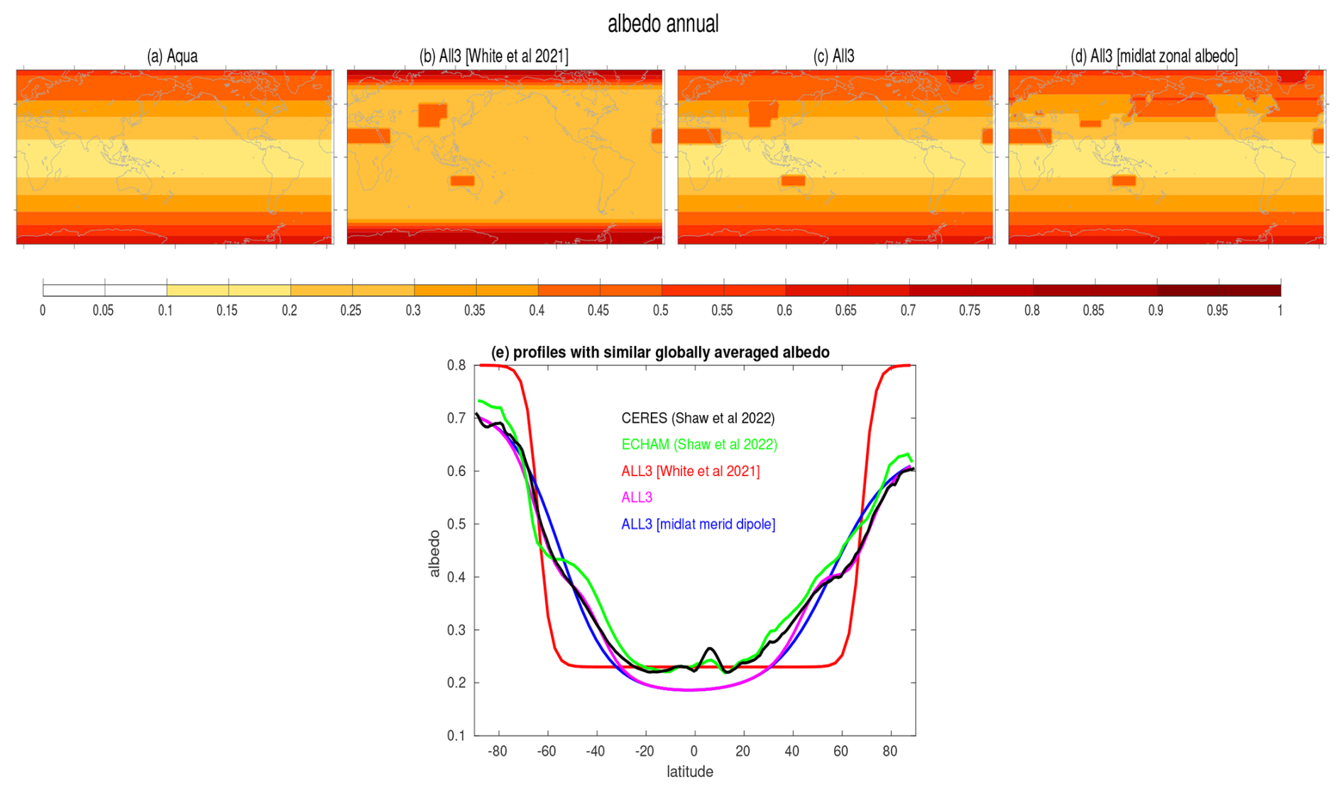
Figure 2 Albedo profiles used in this paper. CERES satellite based albedo is shown in black, and the ECHAM profile from Shaw et al. (2022) with all surface inhomogeneities is in green. The albedo profile from White et al. (2021a) is in red, and also is shown in panel (b), and the storm tracks that arise when using this profile are too weak as compared to ERA5 as discussed in Sect. 3. The updated albedo profile is shown in magenta, and a map view in panel (c); this albedo configuration is used in all runs with land–sea contrast. The albedo for the aquaplanet experiment is shown in panel (a), and this profile is also used in runs without land–sea contrast. Section 6 discusses two sensitivity ALL3 runs where we alter the albedo: the albedo for the case in which we add land–ocean albedo differences is shown in panel (d), and the albedo for the case in which the meridional dipole of Eq. (A2) is not included is shown in blue in panel (e). Note that the albedo in MiMA refers to surface albedo, while in CERES and ECHAM it refers to top of atmosphere albedo.

We therefore use a revised albedo profile in this paper (magenta curve in Fig. 2) that better matches the CERES data, while still using an analytical fit of the form of Eq. (A3) of Garfinkel et al. (2020a), and with a similar global albedo to our previous MiMA work. See Appendix A for details, and Fig. S1 in the Supplement for a comparison of surface temperature in NH midlatitudes to ERA5. Note that the albedo in CERES and ECHAM refers to top of atmosphere albedo, while in MiMA it refers to surface albedo, as there are no shortwave cloud effects in MiMA. The albedo for the aquaplanet experiment is shown in Fig. 2a, and this profile is also used in runs without land–sea contrast.

The second major change made to the configuration of White et al. (2021a) is an adjustment to the ocean heat flux to better account for the net transport of heat from the SH to the NH associated with the meridional overturning circulation in the Atlantic. This adjustment is necessary because the formulation in White et al. (2021a) implies too little transport of heat from the SH to the NH within the ocean, as compared to the observationally derived flux of Shaw et al. (2022). The details of the perturbation are shown in Appendix A. The net effect of the perturbation (when A in Eq. B1 is set equal to 2.1 W m⁻²) is a more realistic implied net heat transport to the NH. Namely, the net heat transport from the SH (20° S-pole) to the NH (20° N-pole) is 0.54 PW, both here and in the observationally derived estimate from Shaw et al. (2022). For reference, the corresponding heat transport over these latitude bands in the White et al. (2021a) configuration is just 0.24 PW, even as it captures the overall spatial pattern. Frierson et al. (2013) inferred an alternative heat transport estimate of 0.4PW from the SH to the NH when integrating over the entire hemisphere, but with large interannual variability. Note that there are even larger differences in the ocean heat transport in other published estimates (compare Trenberth and Fasullo, 2008, 2017, Frierson et al., 2013, Shaw et al., 2022, and Mayer et al., 2024), with substantial sensitivity to methodology in the vicinity of the boundary currents (Mayer et al., 2024).

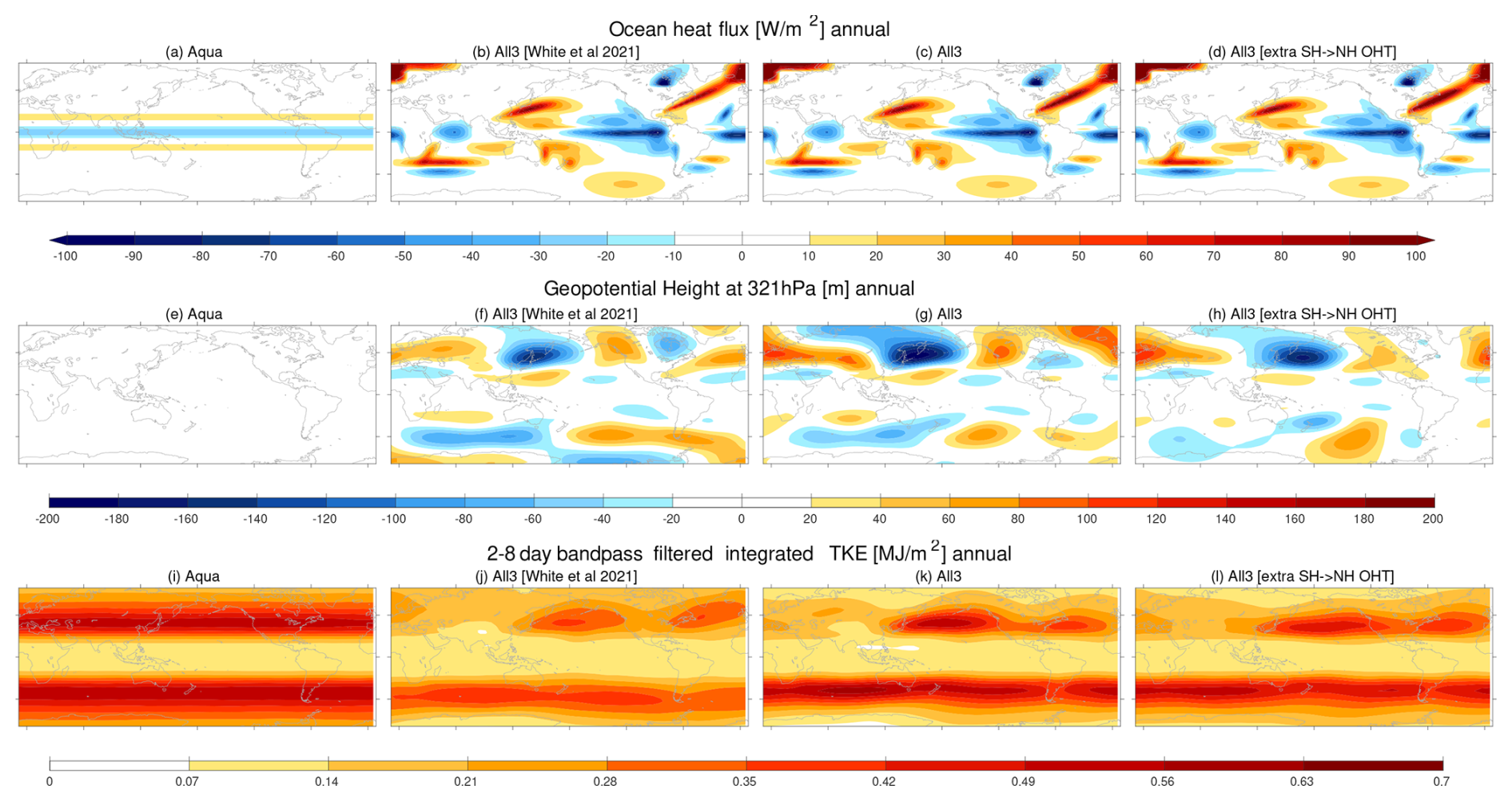
Figure 3 Ocean heat flux used for the (a) aquaplanet configuration (Merlis et al., 2013); (b) the All3 configuration of White et al. (2021a); (c) the updated All3 configuration used in this paper (see Eq. B1); (d) as in panel (c), but with an amplitude factor of 3.5 W m⁻² instead of 2.1 W m⁻² in Eq. (B1). Note that differences among panels (b) to (d) are hard to detect by eye, but are present in the Southern Ocean and North Atlantic. The corresponding stationary wave structure for each configuration is shown in the second row, and the TKE in the third row.

The updated ocean heat flux is shown in Fig. 3c, while the configuration from White et al. (2021a) (with A = 0 W m⁻² and 0.24 PW in interhemispheric transport) is in Fig. 3b. While the difference is difficult to detect by eye, this small change leads to a realistic NH vs. SH asymmetry in the surface energy flux term (as discussed in Sect. 5). In addition to A = 2.1 W m⁻² (with 0.54 PW in interhemispheric transport), we perform sensitivity tests in Sect. 5 in which we set A to 3.5 W m⁻² to further increase the export of heat to the NH to 0.74 PW (Fig. 3d). This higher value of A is intended to explore sensitivity to uncertainty in this difficult-to-observe quantity. The ocean heat flux is steady (not monthly varying). The implications of this simplification are discussed in Sect. 7. Note that all configurations, including the aquaplanet version without any hemispheric asymmetries, have the tropical OHT of Merlis et al. (2013, Fig. 3a).

2.2 Experiments

We evaluate the role of three core surface inhomogeneities – topography (TOPO), land–sea contrast (LSC), and ocean heat transport (OHT) – for storm tracks using the MiMA experiments listed in Table 1. These experiments are similar to those in Garfinkel et al. (2020c) which focused on stationary waves, but with updates in the specification of each of these inhomogeneities as discussed in White et al. (2021a) and Sect. 2.1. Each experiment lasts 38 years after discarding at least 10 years of spinup to achieve a statistical steady state, and so oceanic and atmospheric energy storage do not contribute to differences in the energy budget among the experiments. In addition to these eight experiments, Sect. 6 describes sensitivity ALL3 experiments that explore the role of land–sea and meridional gradients in albedo, and the flux of additional heat to the NH from the SH. All integrations here were run at a horizontal resolution of triangular truncation 42 (T42), although the most realistic configuration was also run at T85 with similar results (see Sect. 3). All integrations were run with 40 vertical levels with a model lid near 70 km.

Table 1 MiMA Experiments, with “Y” indicating an inhomogeneity is on and “N” indicating an inhomogeneity is off. The isolated nonlinear response to topography can be deduced by comparing topography-only to aquaplanet, while the full nonlinear response is the difference between ALL3 and LSC+OHT. The isolated nonlinear response to land–sea contrast can be deduced by comparing LSC-only to aquaplanet, while the full nonlinear response is the difference between ALL3 and TOPO+OHT. The isolated nonlinear response to horizontal gradients in ocean heat flux (with implied changes in ocean heat transport) can be deduced from experiment OHT only as compared to aquaplanet, while the full nonlinear response is the difference between ALL3 and TOPO+LSC. Note that all configurations, including the aquaplanet ones, have the tropical implied OHT of Merlis et al. (2013, Fig. 3a). In addition to these experiments, three sensitivity experiments with ALL3 have been performed in which the albedo profile or the ocean heat flux is modified; these modifications are described in the text.

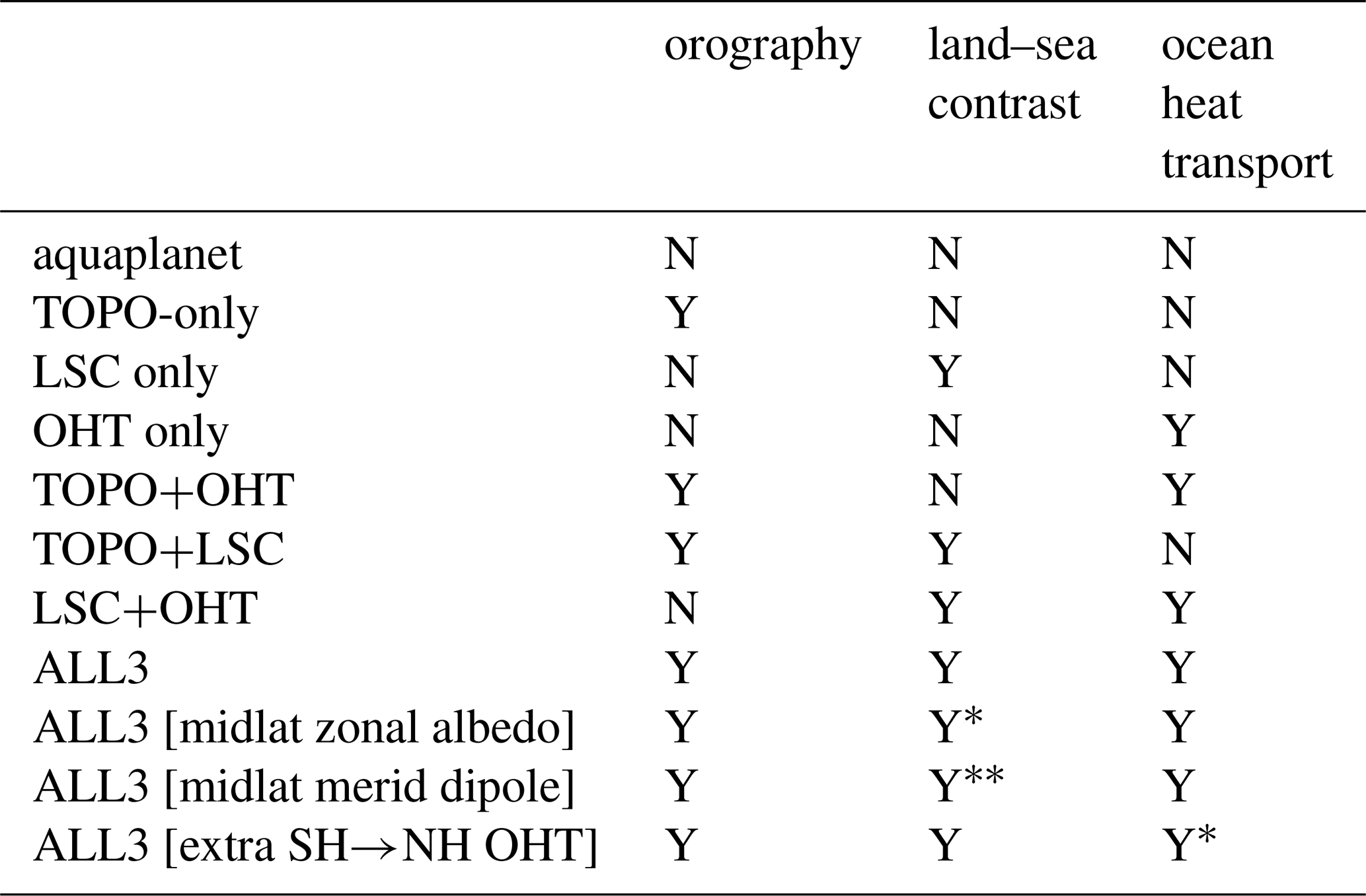
^*, ${}^{**}$ denote that the specification is altered as described in the text.

These experiments can be used to infer the role of each surface inhomogeneity for storm tracks in two complementary ways. Adopting the terminology of Held et al. (2002), these are known as the isolated and full nonlinear response to a given surface inhomogeneity. First, we denote as M(I) the response to some source of inhomogeneity I in MiMA, when compared to a zonally symmetric aquaplanet; this M(I) is called the isolated nonlinear response to I. Next, we let T represent all three inhomogeneities in the most realistic configuration (ALL3), such that the response to T is M(T). As in Held et al. (2002), we can then compute the difference between M(T) and M(T − I), and this response is known as the full nonlinear response to I. If we consider adding the three different inhomogeneities in sequence, the isolated nonlinear response to I occurs when I is added first, while the full nonlinear response to I occurs when I is added last (or is the first to be removed).

Figure S2 demonstrates that the non-additivity noted in Garfinkel et al. (2020c) with regards to boreal winter stationary waves is still evident in these experiments which incorporate the changes of Sect. 2.1.

2.3 Defining storm tracks

We adopt two measures of the storm track activity. The first is transient kinetic energy (TKE), which is computed by applying a 2 to 8 d band-pass 5th order Butterworth filter to u and v, and then computing $u_{\mathrm{hi}}^{\mathrm{2}}+v_{\mathrm{hi}}^{\mathrm{2}}$. We then vertically integrate from the surface (p_s) to the top of atmosphere:

$$\begin{array}{}\text{(1)}& \text{TKE}={\displaystyle \frac{-\mathrm{1}}{\mathrm{2}g}}\underset{\mathrm{ps}}{\overset{\mathrm{0}}{\int }}{u}_{\mathrm{hi}}^{\mathrm{2}}+v_{hi}^{\mathrm{2}}\mathrm{d}p.\end{array}$$

The second measure of storm track activity is motivated by the energy budget framework used in Sect. 5 to diagnose how the three surface inhomogeneities affect the NH vs. SH storm track asymmetry. For this energy budget framework, a more natural definition of storm tracks is the atmospheric moist static energy flux on sub-monthly timescales. We now introduce this energy budget framework. The total (atmosphere plus ocean) meridional heat transport (MHT) across a latitude circle by the coupled (ocean–atmosphere) climate system must, on long time scales, be balanced by the net top-of-atmosphere (TOA) radiative deficit spatially integrated over the polar cap bounded by that latitude circle (e.g., Haar and Oort, 1973, Fig. 4). This constraint helps motivate an energetic framework, in which MHT is equal to the net TOA radiative deficit integrated over the extratropics or, equivalently, the net radiative excess integrated over the tropics (e.g., Barpanda and Shaw, 2017, 2020; Shaw et al., 2018; Donohoe et al., 2020). This statement can be expressed mathematically as

$$\begin{array}{}\text{(2)}& \mathrm{\text{MHT}}\left(\mathit{\varphi }\right)=-\mathrm{2}\mathit{\pi }{a}^{\mathrm{2}}\underset{\mathit{\varphi }}{\overset{\mathrm{pole}}{\int }}\cos \left({\mathit{\varphi }}^{\prime }\right)\left[\text{ASR}\left({\mathit{\varphi }}^{\prime }\right)-\text{OLR}\left({\mathit{\varphi }}^{\prime }\right)\right]\mathrm{d}{\mathit{\varphi }}^{\prime },\end{array}$$

The hemispheric-scale radiative imbalance results from the equator-to-pole gradient of absorbed solar radiation (ASR; dark pink in Fig. 4) being steeper than that of outgoing longwave radiation (OLR, light pink in Fig. 4; Trenberth and Stepaniak, 2004; Oort and Haar, 1976). On subyearly timescales, atmospheric and oceanic storage is a critical part of the energy budget (Barpanda and Shaw, 2020), however we focus on 38-year averages after a long spinup and so storage is not important.

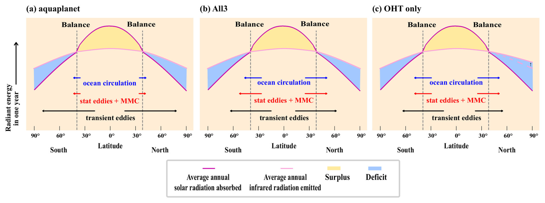
Figure 4 Schematics of the energy budget response in (a) aquaplanet; (b) ALL3; (c) in OHT only. In all configurations, the shortwave term (dark pink) is similar, however the longwave term in panel (c) is higher in the NH than in aquaplanet (see dashed curve in panel c) due to NH surface warming enlarging the energy deficit in the NH extratropics, which then requires an increase in the total NH meridional heat transport. This partially mitigates the effect of stationary eddies and ocean circulation which in isolation induce a weaker NH storm track compared to aquaplanet.

The MHT is typically decomposed into four terms, an ocean heat transport term (OHT; blue in Fig. 4) and an atmospheric heat transport term (AHT) which is further decomposed into contributions from the mean meridional overturning circulation (MMC), stationary eddy flux (SE; red in Fig. 4), and transient flux (TE; black in Fig. 4).

$$\begin{array}{}\text{(3)}& \text{MHT}=\text{OHT}+\underset{\mathrm{AHT}}{\underbrace{\text{MMC}+\text{SE}+\text{TE}}}.\end{array}$$

We calculate the AHT as the zonally and vertically (mass weighted) integrated meridional transport of moist static energy MSE = C_pT + Lq + gZ, where T is the atmospheric temperature, C_p is the specific heat of air at constant pressure, L is the latent heat of vaporization of water, q is the specific humidity, g is the acceleration of gravity, and Z is the geopotential height. The meridional velocity and MSE are subdivided into the zonal and stationary eddy components, and also time-mean and transient components (as in Priestley, 1949). Upon designating zonal averages with square brackets [ ], time averages over each month of analysis with overbars $\stackrel{\mathrm{‾}}{\left(\right)}$, departures from the zonal average with asterisks (^*), and departures from the time average with primes (^′), the time-mean, zonal-mean, and vertically integrated total energy transport is

$$\begin{array}{}\text{(4)}& \stackrel{\mathrm{‾}}{\text{AHT}\left(\mathit{\varphi }\right)}={\displaystyle \frac{\mathrm{2}\mathit{\pi }a\cos \left(\mathit{\varphi }\right)}{g}}\underset{\mathrm{0}}{\overset{p_{\mathrm{s}}}{\int }}[\underset{\mathrm{MMC}}{\underbrace{\left[\stackrel{\mathrm{‾}}{V}\right]\left[\stackrel{\mathrm{‾}}{\text{MSE}}\right]}}+\underset{\mathrm{SE}}{\underbrace{{\stackrel{\mathrm{‾}}{V}}^{*}{\stackrel{\mathrm{‾}}{\text{MSE}}}^{*}}}+\underset{\text{TE}}{\underbrace{\stackrel{\mathrm{‾}}{V^{\prime }{\text{MSE}}^{\prime }}}}]\mathrm{d}p,\end{array}$$

where V is the meridional velocity and the vertical integral is over pressure p from the TOA to the surface. We use 6-hourly instantaneous fields to calculate the energy transport for each month of model simulation, averaging the results over all years to define the climatological AHT. Note that the transient term TE includes all deviations from sub-monthly timescales (both zonal mean and zonally anomalous; V^′ = $V^{\prime *}$ + [V^′]), and deviations are defined relative to its monthly average, that is an average over a particular month not the climatological monthly average (Shaw et al., 2022). For the MMC term, mass conservation is ensured by subtracting from $\stackrel{\mathrm{‾}}{\left[V\right]}$ the pressure weighted vertical integral of meridional velocity at each latitude.

This calculation is performed on the model's native sigma levels to avoid interpolation errors and uses the daily varying latitude versus longitude surface pressure. In MiMA, all of these terms can be computed directly from the model output (as opposed to CMIP model data where typically transients are inferred as the residual of the rest of the terms, Donohoe et al., 2020), and the residual is small as discussed in Sect. 5. This small residual is due to performing the calculation on sigma levels – residuals are a factor of 3 to 4 larger when the calculation is performed after interpolating to standard pressure levels. We apply a 0.65 rescaling factor to all terms in the MSE budget (following Shaw et al., 2022) to allow for a simpler comparison to the TKE perspective of storm tracks. In statistical steady state with no net changes in oceanic or atmospheric storage, the OHT must balance the surface energy exchange, and thus can be computed by summing the evaporation, sensible heat, longwave, and shortwave surface terms.

In MiMA, we dictate the ocean heat transport through our specification of the ocean heat flux. We are also able to control absorbed solar radiation nearly completely via our specification of the albedo (note that atmospheric scattering and absorption are similar in all experiments, and recall that MiMA has no radiatively active clouds). Furthermore, changing the land–sea contrast and topography directly affects surface and atmospheric temperatures, and hence has an immediate impact on longwave radiation emitted. These surface boundary conditions, together with the ocean heat flux, also directly affect the atmospheric stationary eddies. The net effect is that by changing the albedo, the ocean heat flux, the land–sea contrast, and the topography, we exercise control over all of the parameters in Fig. 4 but one: the transient eddies. This enables us to use this budget to causally explain how changes in transient eddies are driven by perturbations to the surface boundary conditions.

$$\begin{array}{}\text{(5)}& \begin{array}{rl}\mathrm{\Delta }\text{TE}& =-\mathrm{\Delta }\text{OHT}-\mathrm{\Delta }\text{MMC}-\mathrm{\Delta }\text{SE}-\mathrm{2}\mathit{\pi }{a}^{\mathrm{2}}\underset{\mathit{\varphi }}{\overset{\mathrm{pole}}{\int }}\cos \left({\mathit{\varphi }}^{\prime }\right)\\ & \left[\mathrm{\Delta }\text{ASR}\left({\mathit{\varphi }}^{\prime }\right)-\mathrm{\Delta }\text{OLR}\left({\mathit{\varphi }}^{\prime }\right)\right]\mathrm{d}{\mathit{\varphi }}^{\prime },\end{array}\end{array}$$

This ability to relate surface inhomogeneities to storm track strength allows for a causal interpretation of storm tracks (Barpanda and Shaw, 2020). Specifically, Shaw et al. (2022) showed the SH vs. NH asymmetry could be connected to TOA radiation, surface fluxes and stationary circulation energy transport. Unfortunately, frameworks based on mean temperature cannot be easily related to these inhomogeneities, however changes in temperature are nonetheless helpful in understanding localization of storm tracks and are included in Sect. 7.

3 Realism of MiMA storm tracks

We begin by comparing the storm tracks in MiMA to those in ERA5. Figure 1 contrasts the vertically integrated 2–8 d filtered transient kinetic energy (Eq. 1) in ERA5 and in several configurations of MiMA with all three surface inhomogeneities. Observed storm tracks peak in the North Pacific and North Atlantic, and in the Southern Ocean in the Indian Ocean sector. This zonal structure is captured by MiMA. At T85, the zonal structure of the storm tracks in the SH is well captured and the land vs. ocean storm track asymmetry in the NH is also captured realistically, however, MiMA simulates a too-strong storm track in the North Pacific and a too-weak storm track in the North Atlantic (compare Fig. 1a to Fig. 1b). At T42, MiMA struggles to capture certain aspects of the zonal structure of the storm track in the SH: the Indo-Atlantic sector SH storm track should be stronger than the SH Pacific sector storm track (compare Fig. 1a to Fig. 1d). That is, it correctly predicts that the Indian Ocean sector should have stronger storms, but cannot capture the fact that the Atlantic is stormier than the Pacific. The T42 configuration also underestimates the southwest-northeast tilt of the storm track in the North Atlantic.

The White et al. (2021a) configuration underestimates storm track strength in both hemispheres, but especially in the SH. While the storm tracks in the White et al. (2021a) configuration at T85 are too weak by 17 % (compare Fig. 1a to Fig. 1e) the bias reaches 29 % at T42 (compare Fig. 1a to Fig. 1c). In contrast, the storm track strength in the ALL3 configuration with all of the updates from Sect. 2 at T85 is realistic, though 7 % too weak at T42 (Fig. 1d). When storm track strength is measured using the transient MSE flux, storm tracks in MiMA are 14 % too strong (Table 2) even as biases in TOA input are less than 3 %. This is because the surface, MMC, and stationary eddy energy fluxes are still too weak even after the updates we have made, with biases especially pronounced in the SH. This bias in the MSE budget in the updated MiMA ALL3 configuration is similar to those in CMIP models (Fig. 4 of Donohoe et al. (2020)). Overall, the updated version of MiMA introduced in Sect. 2.1 (i.e., Fig. 1b, d) is a reasonable tool to use to tackle the question of how surface inhomogeneities interact to give localized storm tracks.

Table 2 Climatology of the terms contributing to the MSE budget in MiMA ALL3 and in ERA5, area-weighted average from 20° to the pole [PW]. See Fig. 4 of Donohoe et al. (2020) for the analog in CMIP models – the overestimate of transient MSE flux in the upated MiMA ALL3 configuration is similar to that in CMIP, as is the larger bias in the SH.

4 The role of the surface inhomogeneities for the zonal structure of storm tracks

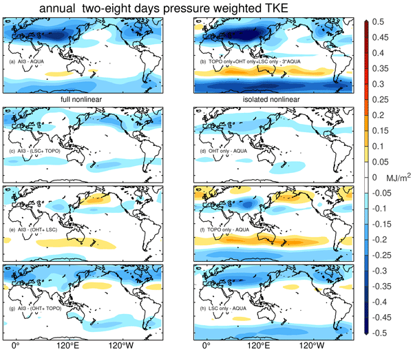
Figure 5 shows the annual averaged climatological storm tracks in the core MiMA runs from Table 1 using a 2–8 d bandpass filter (Eq. 1). In the aquaplanet run (Fig. 5a) the storm tracks lack zonal structure and are nearly symmetric between the hemispheres (note that the albedo profiles are zonally but not hemispherically symmetric; Fig. 2), however, this symmetry is broken in the rest of the panels. The role of realistic OHT can be inferred in two complementary ways. First, the response in the experiment with OHT turned on but all other surface inhomogeneities off (Fig. 5b) can be compared to the response in the Aquaplanet run (Fig. 5a) to infer the isolated nonlinear response: this difference is shown in Fig. 6d. Second, we can compare the experiment with all three boundary inhomogeneities on (Fig. 5e) to the experiment with topography and land–sea contrast on but realistic OHT off (Fig. 5f) to infer the full nonlinear response: this difference is shown in Fig. 6c. In both Fig. 6c and d, adding realistic OHT acts to weaken atmospheric storm tracks (as we might expect since the OHT is poleward) with the effect more pronounced in the NH (for reasons to be discussed in Sect. 5). The regional structure of the changes in the NH are qualitatively different between Fig. 6c and d. The weakening of storm tracks in the full nonlinear response is localized over the North Pacific and North Atlantic, while in isolated nonlinear response the weakening is most pronounced over Eurasia.

Figure 5 Two to eight day bandpass filtered transient kinetic energy (Eq. 1) for each of the runs described in Table 1.

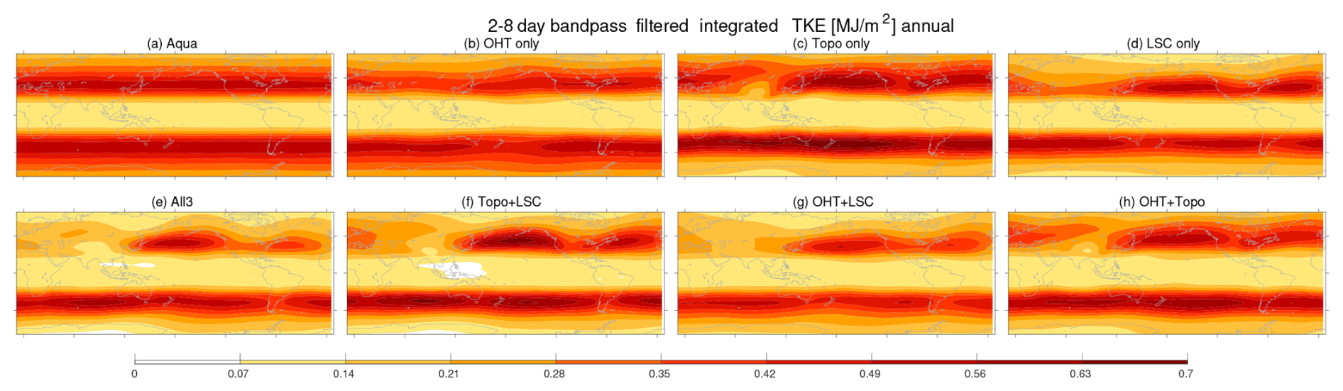
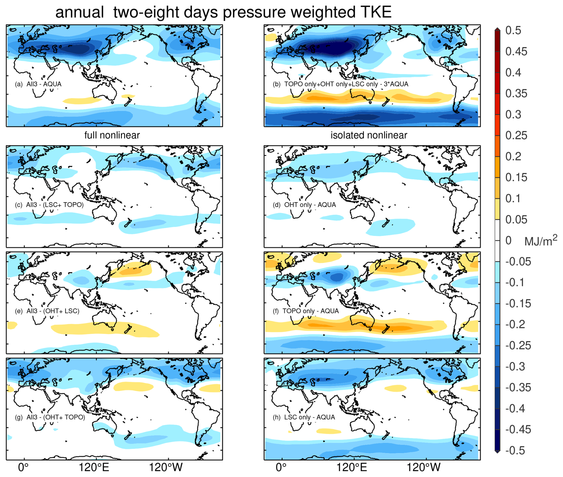
Figure 6 (a) Annual averaged and pressure integrated transient kinetic energy after bandpass filtering u and v for 2 to 8 d (Eq. 1) in ALL3 minus Aquaplanet. (b) As in panel (a), but for the sum of integrations with topography only, land–sea contrast only, and ocean heat transport only, each compared to aquaplanet. (c) The difference between ALL3 and the integration with land–sea contrast and topography. (d) The integration with only ocean heat transport as compared to aquaplanet. (e) The difference between ALL3 and the integration with ocean heat transport and land–sea contrast. (f) The integration with only topography as compared to aquaplanet. (g) The difference between ALL3 and the integration with ocean heat transport and topography. (h) The integration with only land–sea contrast as compared to aquaplanet. Figure S3 shows the analogous figure but for a submonthly filter.

Next, we consider the effect of topography on storm tracks, and begin by contrasting the experiment with topography turned on but all other surface boundary inhomogeneities off (Fig. 5c) to the response in the Aquaplanet run (Fig. 5a) to infer the isolated nonlinear response (Fig. 6f). Topography dampens storm tracks both over the Tibetan Plateau and the Southern Ocean. The weakening over the Southern Ocean also projects onto an equatorward shift of storm tracks (consistent with Patterson et al., 2020). This damping is also evident in the full nonlinear response (Fig. 5e minus Fig. 5g) shown in Fig. 6e, however, the effect is weaker by more than a factor of two and over a limited spatial extent. The large role of topography for SH storm tracks is consistent with Singh et al. (2016) and Patterson et al. (2020), and the dampening of storm tracks over the Tibetan Plateau and subtropical North Pacific, but strengthening downstream, are consistent with Manabe and Terpstra (1974) and Fig. 7 of Lee et al. (2013).

Finally, we consider the effect of land–sea contrast. The isolated nonlinear response (Fig. 5d minus Fig. 5a) is shown in Fig. 6h and indicates that land–sea contrast weakens the storm tracks over the Southern Ocean, Eurasia, and North America, but with a minor effect on the North Atlantic storm tracks. In contrast, the full nonlinear response (Fig. 5e minus Fig. 5h), shown in Fig. 6g, suggests that land–sea contrast has minimal impact on storm tracks in the Southern Ocean, but weakens storm tracks in the North Atlantic.

The non-additive behavior is summarized by contrasting the response to all three surface inhomogeneities (Fig. 5e minus Fig. 5a; Fig. 6a) to the sum of the individual responses to each of the surface inhomogeneities when imposed on an aquaplanet (Fig. 6b). The effect of the surface inhomogeneities is magnified when imposed on an aquaplanet as compared to when they are taken away from ALL3 in most sectors; that is, anomalies in Fig. 6b are larger in magnitude over all sectors than in Fig. 6a. All three building blocks are important for localizing storm tracks, with land–sea contrast the most important in most regions for the full nonlinear response (except near and downstream of the Tibetan Plateau where topography contributes), and topography and land–sea contrast roughly equally important for the isolated nonlinear response. All of these effects are evident both for the 2-to-8 d storm track definition and for a sub-monthly definition (Fig. S3). In all cases, adding zonal asymmetries reduces the TKE. Such an effect is to be expected: if the asymmetries do not change the TOA balance too much and always increase the stationary wave component, it follows that the TKE must be reduced. Adding realistic OHT also directly increases the ocean contribution to poleward flux, so again, the response of TKE is negative. This naturally leads to stronger storm tracks in the SH than in the NH. The next section quantifies these energy budget perturbations to better understand the hemispheric asymmetries.

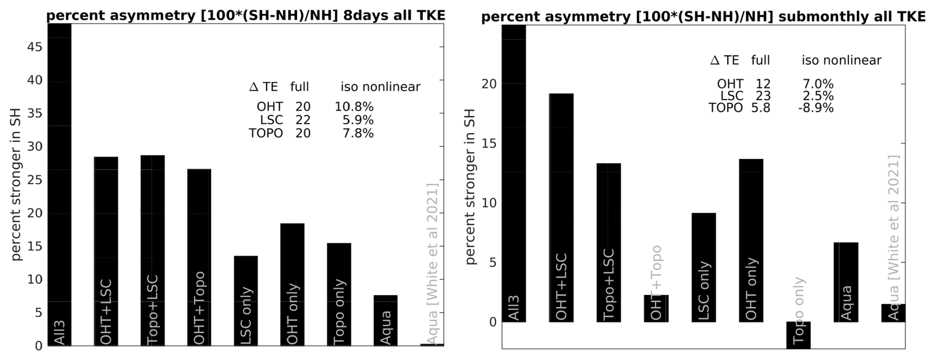
Figure 7 Asymmetry in transient kinetic energy (Fig. 1) between the SH and NH area-weighted from 20 to the pole for a (left) 2–8 d filter and (right) sub-monthly filter for each of the experiments in Table 1. The full nonlinear and isolated nonlinear response to each building block is indicated. A corresponding figure but for the White et al. (2021a) configuration is shown in Fig. S4.

5 Why are SH storm tracks stronger than NH storm tracks?

5.1 Transient kinetic energy perspective

The asymmetry in storm track strength between the SH and NH is summarized for each configuration in Fig. 7. Storm tracks are 48 % and 25 % stronger in the SH for 2–8 d filtered and sub-monthly filtered transient kinetic energy, respectively, in general agreement with Shaw et al. (2022). As surface inhomogeneities are removed, the asymmetry declines. Even in the presence of just land–sea contrast (LSC-only), however, the asymmetry still has not been eliminated (e.g., 9.1 % for submonthly). Part of the asymmetry is due simply to the albedo profile: there is an asymmetry of 6.6 % to 7.5 % (for a submonthly filter and 2–8 d bandpass filter, respectively) in the aquaplanet run with the updated albedo profile in Fig. 2, as compared to the albedo profile used for White et al. (2021a) in which the asymmetry is less than 1.5 %. This asymmetry can be explained by the fact that while the hemispherically averaged albedos are similar in both hemispheres, the subpolar albedo is higher in the SH than in the NH in the updated configuration and in CERES (Sect. 2.1, Fig. 2), and so the meridional gradient in net energy input is larger in the SH (an effect we will quantify shortly using the energy budget). For most experiments results are similar whether we define transient kinetic energy using a 2–8 d filter or a sub-monthly filter. However, for runs with land–sea contrast off but topography on (particularly topography-only, and to a lesser degree OHT+topography) some of the topographically forced quasi-stationary waves are included in the transient eddies category for a sub-monthly definition, leading to stronger storm tracks in the NH.

When considering the 2–8 d bandpass filtered kinetic energy, the most important surface inhomogeneity for the asymmetry is OHT for the isolated nonlinear response (i.e. when comparing to AQUA), while all three have roughly equal contribution for the full nonlinear response (when each is removed from ALL3). However there is substantial non-additivity: the sum of the full nonlinear responses is 30 % larger than the actual asymmetry of 48 % in All3. In contrast, the sum of the isolated nonlinear responses is only 25 %, which is only half of the actual asymmetry in All3 of 48 %. Hence, surface inhomogeneities have a bigger impact on the NH vs. SH asymmetry when they are subtracted from ALL3, and a weaker impact when they are added to AQUA. This effect is opposite to what we saw in Sect. 4 with regards to regional impacts: the surface inhomogeneities have a bigger impact on regional storm tracks when they are added to AQUA than when subtracted from ALL3.

5.2 Moist static energy perspective

The moist static energy budget introduced in Sect. 2.3 is now used to explain why the SH storm tracks are stronger than the NH storm tracks. We begin by showing the terms of the MSE budget for the aquaplanet and ALL3 configurations in Fig. 8. Figure 8a shows the net energy input, and as expected energy accumulates in the tropics while there is a deficit in the extratropics (e.g., Fig. 4). For a given albedo profile, the TOA terms are similar between ALL3 and aquaplanet (Fig. 8b), while changing the albedo profile has a large effect on the TOA radiative terms (not shown). In contrast, changing the ocean heat flux between the idealized configuration for an aquaplanet (Fig. 3a) and any of the more realistic configuration leads to a large change in the surface energy input (Fig. 8c).

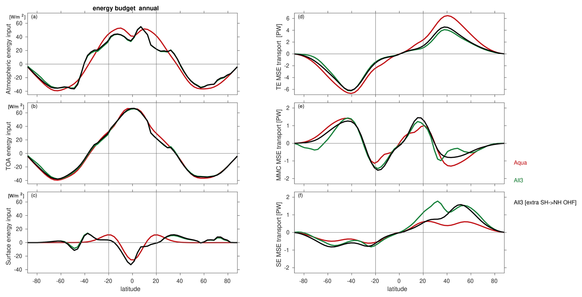
Figure 8 Annual-mean atmospheric energy transport in three representative MiMA simulations. (a) Atmospheric energy input, which in turn is the sum of the (b) top of atmosphere energy input (shortwave minus longwave) and (c) surface energy input (latent+sensible+shortwave+longwave, which must balance the ocean heat transport in steady state). (d) Transient MSE transport; (e) mean meridional circulation MSE transport; (f) stationary eddy MSE transport. Note that the range on the y axis differs between panels (d), (e), and (f). All the left-hand panels have the same range on the y axis. Compare to Fig. 5 of Donohoe et al. (2020) for observational and CMIP analogs. For panels (a) through (c) we multiply by cos (ϕ) before plotting (see Eq. 2).

The integrated energy input from latitude ϕ to the pole must be balanced by the energy transport at that latitude (Eq. 2), and these energy transport terms are shown in the right column of Fig. 8. The poleward energy transport is dominated by transient eddies (Fig. 8d), and these transient eddies are stronger in the NH for the aquaplanet configuration than for the ALL3 configuration (Fig. 4a, b). Conversely, the stationary eddy terms are stronger in the ALL3 configuration than in the aquaplanet configuration (Fig. 8f), such that there is a hand-off from transient to stationary eddies that keeps net MSE transport quantitatively similar to balance the similar energy input (Figs. 8a; 4a, b). Note that we compute all terms explicitly from the model output – none are inferred as residuals.

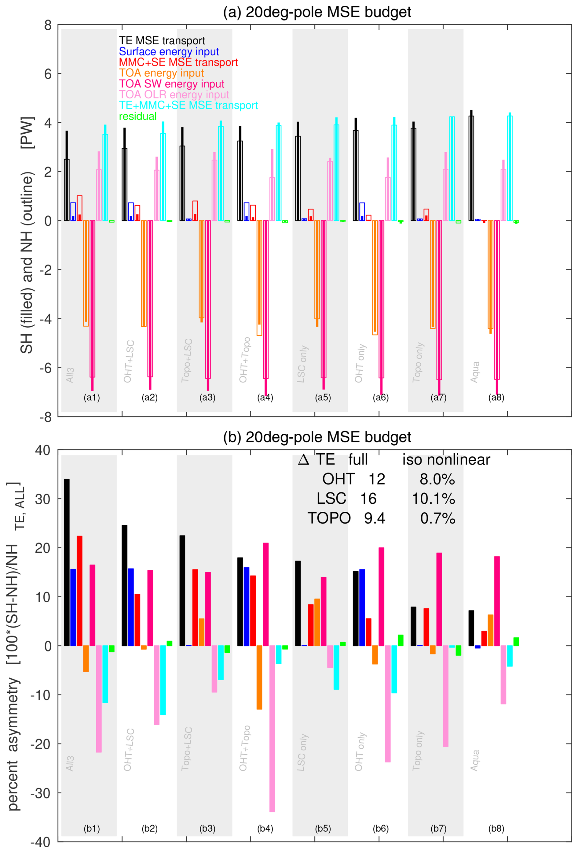
Figure 9 Moist static energy budget averaged from 20° to the pole (Eq. 2). In panel (a), we show each term for the SH (narrow filled bar) and NH (wide outline-only bar) separately, and in panel (b) the percent difference with the transient term in the NH taken in the denominator (e.g., the OLR percent difference is $\frac{{\text{OLR}}_{\mathrm{SH}}-{\text{OLR}}_{\mathrm{NH}}}{{\text{TE}}_{\mathrm{NH}}}$). For simplicity in our plots we lump together ΔMMC with ΔSE. Panel (b) also summarizes the NH vs. SH asymmetry in sub-monthly MSE flux in response to each surface inhomogeneity for both the isolated and full nonlinear responses. A similar figure but for the White et al. (2021a) configuration is shown in Fig. S5.

Next, we quantify how each of the surface inhomogeneities affects each of the terms in the MSE budget, and thus can explain the changes in the hemispheric-averaged transient MSE flux. To do this, we apply Eq. (5) to all latitudes from 20° to the pole in both hemispheres, and then take the area-weighted average from 20° to the pole. For context, Shaw et al. (2022) applied this identical framework to reanalysis data and ECHAM, and showed that the Southern Hemisphere is 24 % stormier than the Northern Hemisphere across reanalysis data sets. Furthermore, the MSE budget based storm track asymmetry climatology (rescaled to match the EKE) in ERA5 is 23 % and can be diagnostically decomposed into a 12 % contribution from surface energy fluxes, a 14 % contribution from stationary circulation atmospheric energy flux, and a small −3 % contribution from TOA radiative fluxes. The net energy flux in each hemisphere in MiMA (SH filled and NH outline) is shown in Fig. 9a, with the percentage difference between the hemispheres in Fig. 9b. In ALL3, the SH is 34 % more stormy by this metric (black bar), and of this 15.6 % is due to the surface energy input (blue bar; that is, the ocean fluxes more heat poleward in the NH than in the SH) and 22.4 % to stationary eddies/MMC (red bar; that is, stationary eddies are stronger in the NH than in the SH). Note that this suggests MiMA has a different MSE budget based storm track asymmetry climatology than ERA5 as it places more weight on the stationary eddy contribution. The top of atmosphere term contributes −5.2 %, such that the TOA energy deficit is slightly larger over the NH than the SH and thus partially mitigates the effects of ocean and stationary eddy fluxes. The residual of the MSE budget (green bars) are a factor of 10 less than the smallest term, and so the energy budget is essentially closed. The residuals are similarly tiny (≤ 0.12 mPW per hemisphere) for all of the other experiments when we sum up the energy terms in each hemisphere.

The SH vs. NH asymmetry in TE drops to 24.5 % if we flatten topography but keep OHT and LSC (black in Fig. 9b2). This reduction is due to a reduction in the stationary eddy term (red in Fig. 9b2) as NH stationary waves weaken (red in Fig. 9a2), however the change in the NH vs. SH asymmetry of the TE term (black in Fig. 9b1, b2) is mitigated somewhat by changes in the TOA term (orange in Fig. 9b1, b2), whereby the TOA deficit is now nearly identical in the SH and NH (orange in Fig. 9b2).

If we remove realistic OHT but keep LSC and topography (Fig. 9b3), the SH vs. NH asymmetry in TE drops from 34 % to 22.4 %. This reduction is mostly due to zeroing out of the surface term (as expected, blue bar in Fig. 9b3), however the stationary eddy term also weakens (from 22.4 % to 15.5 %) as some of the stationary eddy energy transport is set up by wavetrains forced by sea surface temperature gradients arising from the ocean heat flux (Fig. 3). The increase in TE in the NH vs. the SH is partially mitigated by changes in the TOA term (orange in Fig. 9b3): in ALL3 the TOA deficit was larger in the NH, but in TOPO+LSC the TOA deficit is larger in the SH (orange in Fig. 9a1 and a3). This change in the sign of the contribution of the TOA term is consistent with the ECHAM experiments of Shaw et al. (2022), though the effect is stronger here in MiMA. This change in the TOA term is almost entirely due to changes in longwave (light pink) rather than shortwave (dark pink). Namely, TOA shortwave energy input is essentially identical in all experiments (dark pink in Fig. 9a) due to the specified albedo profile, while TOA longwave is not (light pink in Fig. 9a).

If we remove LSC but keep OHT and topography (Fig. 9b4), the SH vs. NH asymmetry in TE drops from 34 % to 17.9 %. This reduction by half is not because of changes in the surface energy term (which are unchanged), and changes in the stationary eddy term are even more pronounced when we remove OHT but keep LSC and topography (red bar in Fig. 9b2 vs. Fig. 9b4). The dominant reason for this reduction is, instead, from the TOA asymmetry: the NH TOA deficit grows when LSC is removed – opposite to Fig. 9b2 and b3 – due to the outgoing longwave radiation term (orange and light pink bars in Fig. 9b4).

The remaining panels of Fig. 9 focus on the isolated nonlinear response when each building block is added onto an aquaplanet configuration. As for the full nonlinear response, the most important individual surface inhomogeneity for the NH vs. SH asymmetry in storm track strength is LSC. When LSC is added onto an aquaplanet (Fig. 9b5), NH TE weakens while stationary eddies strengthen, however changes in the TOA term (orange) are equally important to the changes in stationary eddies. Adding LSC leads to less TOA OLR in the NH (light pink), and hence less overall heat transport is needed in the NH, which accentuates the NH vs. SH asymmetry. For the other two isolated nonlinear responses, the TOA term acts as a negative feedback on the increase in the NH vs. SH asymmetry in TE, rather than contributing to it as it does for LSC. For example, adding OHT to an aquaplanet leads to an increase in extratropical NH TOA OLR, which subsequently increases the NH extratropical energy deficit and thus partially mitigates the reduced TE that is needed in response to increased OHT (Figs. 9a6, 4c).

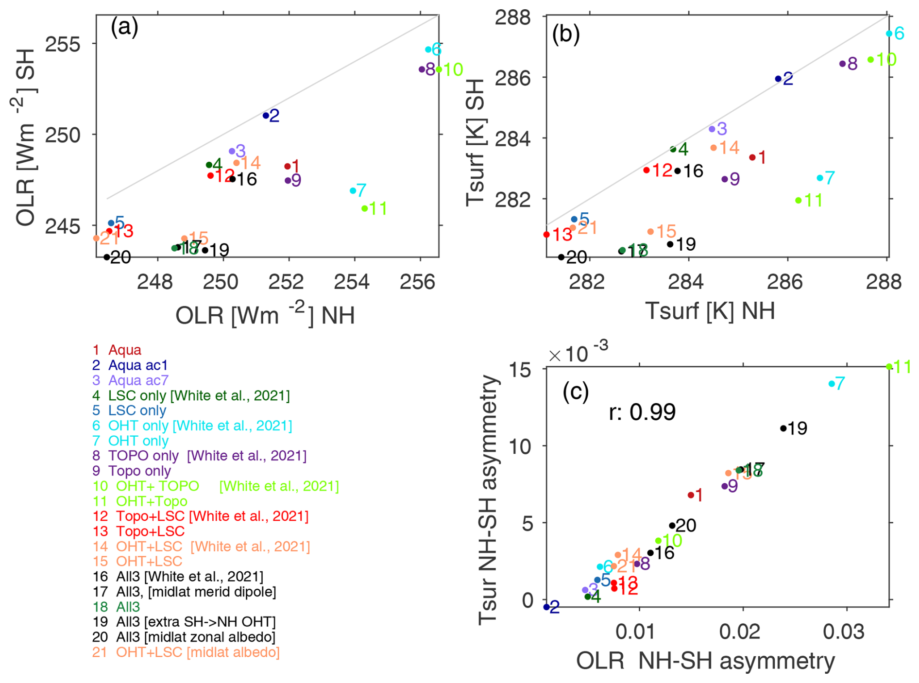
Figure 10 Understanding the TOA NH/SH asymmetry among the various runs. (a) Annual averaged area-weighted OLR from 20° to the pole in each hemisphere; (b) annual averaged area-weighted surface temperature from 20° to the pole in each hemisphere; (c) NH vs. SH asymmetry in OLR (panel a) vs. NH vs. SH asymmetry in surface temperature (panel b). The asymmetry is defined as $\frac{X_{\mathrm{NH}}-N_{\mathrm{SH}}}{X_{\mathrm{SH}}}$ where X refers alternately to OLR or surface temperature. A one-to-one line is include in panels (a) and (b).

Thus far, we have shown that the surface energy input and stationary eddy terms are the most important contributors to the SH vs. NH asymmetry in storm track strength in All3. Nonetheless, changes in the TOA energy output are not insignificant, and act to intensify the asymmetry when LSC is added yet reduce the asymmetry when topography or especially OHT are added. We now turn our attention to why the NH vs. SH asymmetry in the TOA term differs so strongly among these three surface inhomogeneities, and specifically we demonstrate its tight connection to hemispheric averaged surface temperature. Figure 10a shows the area-weighted OLR from 20° to the pole in each hemisphere in all experiments included in this paper, and we also include the corresponding core 8 simulations using the White et al. (2021a) configuration to demonstrate statistical robustness. Consistent with Fig. 9, OLR is higher in the NH than in the SH in all simulations except for an aquaplanet configuration with completely symmetric albedo profiles (labeled “2- Aqua ac1”), but the magnitude of the SH vs. NH asymmetry in OLR differs across the experiments.

To explain this asymmetry in OLR, we next turn to the asymmetry in area-weighted surface temperature from 20° to the pole in each hemisphere (Fig. 10b). The NH is warmer than the SH in nearly all simulations, with the asymmetry smaller in aquaplanet runs or in runs with only land–sea contrast (runs 2 through 5). That is, both topography and ocean heat transport act to cool the SH more than the NH, while land–sea contrast cools both hemispheres nearly equally.

The importance of the surface temperature asymmetry for the OLR asymmetry is quantified in Fig. 10c. Across all 21 simulations, the correlation between the OLR and the surface temperature asymmetries is 0.99, and hence surface temperature asymmetries dictate OLR asymmetries in MiMA. The corresponding correlation with ocean heat transport or albedo is much lower (0.79 and 0.64). The asymmetry in surface temperature is particularly large in runs with OHT on but land–sea contrast off (runs 7 and 11), and also is enhanced using the updated OHT profile vs. the White et al 2021 profile, and even more-so when we amplify the OHT perturbation (ALL3 [extra SH→NH OHF], run 19). Of the three surface inhomogeneities, LSC tends to have a muted impact on the hemispheric asymmetries in surface temperatures and if anything preferentially cools the NH (runs 2 through 5 are near the origin in Fig. 10c), while the other two increase it and preferentially cool the SH (with the effect particularly strong for OHT, which warms the NH much more than the SH). Hence, the changes in the TOA term in Fig. 9 can be explained by the effect of each building block on surface temperature. These sensitivities appear to be larger than in the simulations of Cox et al. (2022) in which idealized orograpy is added to an aquaplanet.

Overall, the storm tracks in the SH are stronger than those in the NH. All three surface inhomogeneities contribute to this asymmetry, but the contributions are unequal. The most important contributor is land–sea contrast, the second most important is ocean heat flux, while topography is the least important contributor. This relatively small role for topography is particularly pronounced when using a sub-monthly definition for storm track intensity (Fig. 6). Topography has a pronounced role only in the vicinity of the Tibetan Plateau, but in the zonal mean this effect is relatively weak. Most of the change in transient MSE flux as surface inhomogeneities are removed can be explained by the stationary eddies (for all three surface inhomogeneities) and surface terms (for ocean heat transport). These surface inhomogeneities also influence the hemispheric averaged surface temperature, and the subsequent effect on outgoing longwave radiation changes explains the rest of the change in transient MSE flux. Specifically, adding OHT acts to preferentially warm NH subpolar latitudes more than SH subpolar latitudes, which partially mitigates the effect of OHT on the SH vs. NH storm track asymmetry that would occur if just the stationary eddy and surface terms were present. In contrast, land–sea contrast acts to preferentially cool NH subpolar latitudes more than SH subpolar latitudes, which intensifies the effect of LSC on the SH vs. NH storm track asymmetry beyond what would occur if just the stationary eddy term was present.

6 Sensitivity to the specification of the albedo and ocean heat flux

The two most crucial changes made to the model configuration from White et al. (2021a, see Sect. 2.1) are in the specification of the SH to NH ocean heat transport and to the extratropical albedo, and we now consider the importance of these changes for the NH vs. SH asymmetry in storm track strength. We begin with the integration with an enhanced ocean heat flux from the Southern Ocean to the North Atlantic (Fig. 3d) with A set equal to 3.5 W m⁻² instead of 2.1 W m⁻² in Eq. (B1), thereby increasing the interhemispheric ocean heat transport to 0.74 PW from 0.54 PW (i.e., a 0.1 PW reduction in flux to the extratropical SH, and a 0.1 PW increase in flux to the extratropical NH). One would naively expect that transient kinetic energy should strengthen in the SH and weaken in the NH, as the ocean is now fluxing less heat to subpolar latitudes in the SH, but fluxing more heat to subpolar latitudes in the NH (see blue bars in Fig. 11a2).

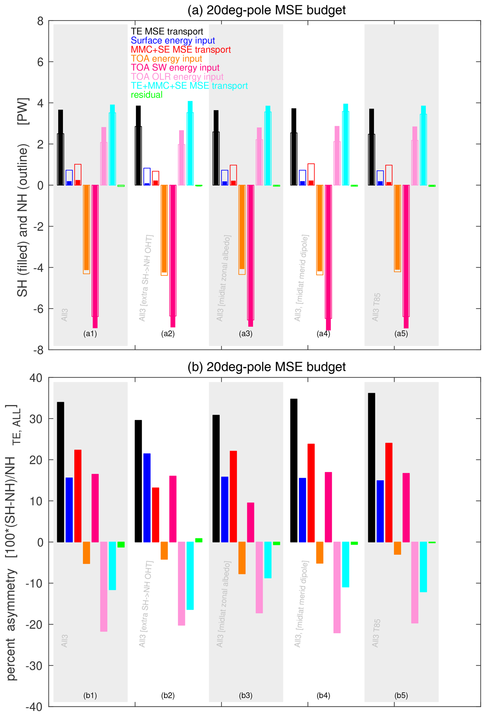
Figure 11 As in Figure 9 but for runs isolating the role of the extra SH to NH ocean heat flux, for runs changing the midlatitude albedo profile, and ALL3 at T85. First we show SH and NH separately, and then below the percent difference. A TKE perspective on the hemispheric asymmetry is shown in Fig. S6.

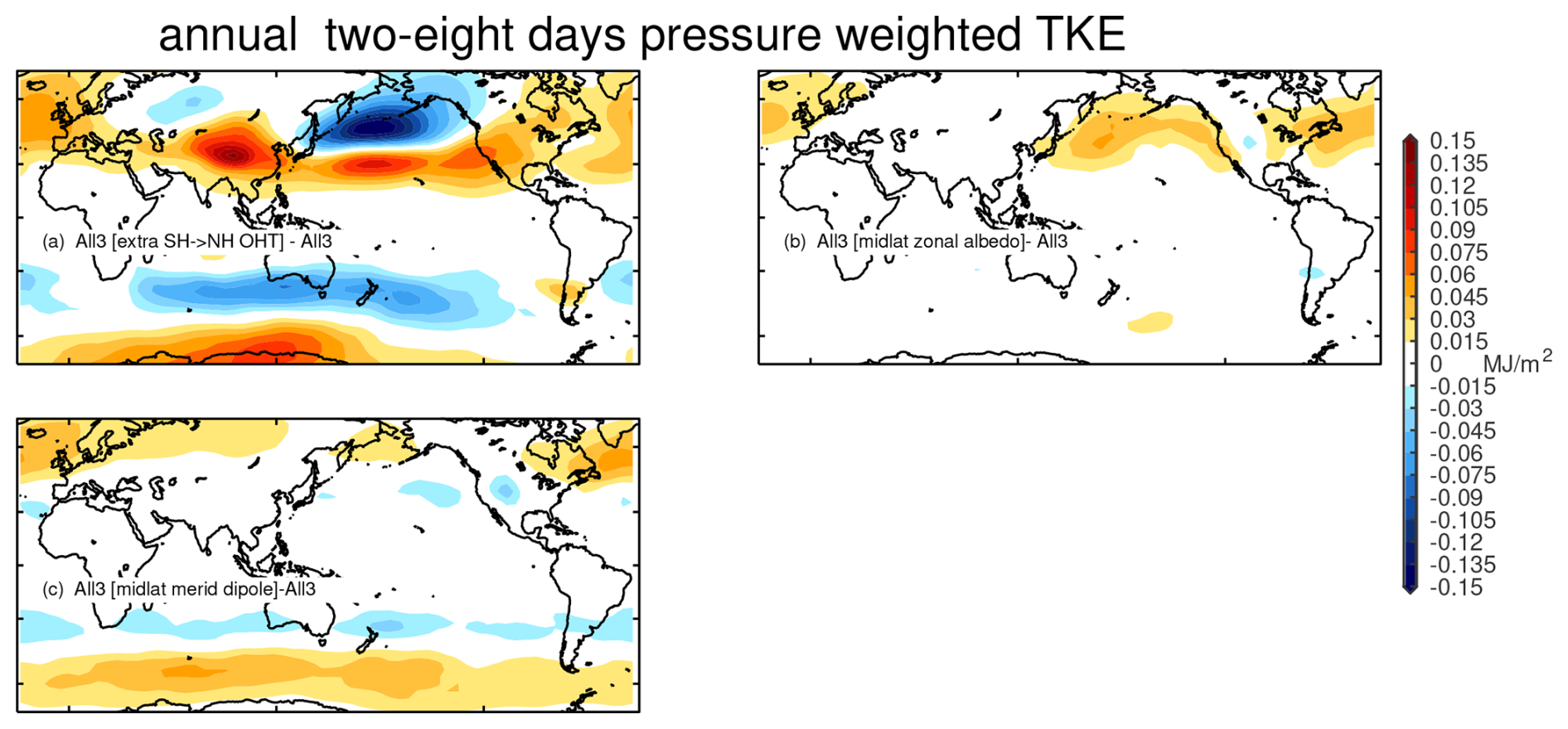
Figure 12 As in Fig. 6 but for runs exploring the response to (a) extra SH→NH ocean heat flux, or to a (b) zonal or (c) meridional perturbation to the albedo in midlatitudes.

In the SH, this is exactly what happens: the ocean heat transport decreases by 0.1 PW while the TE heat transport increases by the same amount (to within 10 %). In the NH, however, the 0.1 PW increase in ocean heat transport does not lead to a reduction in TE heat transport, and in fact the opposite occurs: TE heat transport increases by 0.34 PW. Rather, the biggest change in the energy budget in the NH in response to the ocean heat flux perturbation is in the stationary eddy term, which decreases by 0.34 PW in the NH (red bars in Fig. 11a2). The MMC term is essentially unchanged (not shown) while the change in the TOA deficit (orange bars) is 0.09 PW, so the increase in TE in the NH is needed primarily to balance the weakening of stationary eddy activity. This weakening of stationary wave activity is also evident when examining the deviation of 321 hPa (model level closest to 300 hPa) geopotential height from its zonal mean (Fig. 3g, h) in all sectors of the NH. Namely, the Northwest Pacific trough, the western North American ridge, the Hudson Bay trough, and the North Atlantic ridge, all weaken when the ocean heat flux to the NH is increased.

Figure 3k, l allows for isolating the specific sectors in which transient kinetic energy increases in response to this enhanced ocean heat flux to the North Atlantic, and most of the increase in TE kinetic energy occurs in the North Atlantic (Fig. 3k vs. l). This local intensification of TE kinetic energy in response to a more pronounced Gulf stream is consistent with previous work demonstrating that ocean SST gradients invigorate storms and blocks locally (Brayshaw et al., 2011; Booth et al., 2012; Wenta et al., 2024). This local Atlantic sector increase drives the increase in hemispheric TE, as TE actually decreases in the Pacific sector (Fig. 12a). While the energy budget can successfully diagnose these changes, it does not appear capable of providing a causal explanation that directly links the ocean heat flux changes to transient kinetic energy, as it cannot predict changes in stationary wave amplitude. The net effect is a decrease in the hemispheric asymmetry of the storm tracks, and this is evident both for the MSE TE flux and for TKE (Figs. 11b and S5).

Next, we consider the integration with lower albedo over midlatitude NH continents and higher albedo over the ocean (Fig. 2d). Specifically, between 35 and 60° N, albedo over ocean gridpoints is increased by 0.1, while albedo over land is decreased by 0.03; this perturbation resembles that seen in the ECHAM6 runs of Shaw et al. (2022), and slightly exaggerates the asymmetry in CERES data (not shown). This change leads to an increase of 0.0125 in NH area-weighted average albedo from 20° N to the pole, and so would be expected to strengthen NH storm tracks. Such a strengthening of NH storm tracks indeed occurs: in the NH the submonthly MSE flux increases by 0.08 PW in this run (black bars in Fig. 11a3). This increase is associated with the TOA term: net shortwave absorbed in the NH decreases (dark pink). However, the change in the submonthly MSE flux forced by this reduction in albedo and in absorbed shortwave is mitigated by a corresponding decrease in OLR. Namely, OLR also decreases by nearly the same amount as the shortwave term, due to a colder NH (light pink; see also marker 20 vs. 18 in Fig. 10), and so the net TOA deficit (orange) in the NH increases only slightly. The slightly more pronounced shortwave reduction (as compared to the OLR decrease) explains the residual decrease in the NH vs. SH asymmetry, while the stationary eddy and surface terms are unchanged. While hemispheric mean changes are small, there is pronounced zonal structure to the storm track response: NH storm tracks strengthen in the North Pacific and North Atlantic (Fig. 12b), as expected as the albedo is decreased in these regions.

Finally, we consider the experiment in which the meridional dipole in albedo described by Eq. (A2) is not included (blue in Fig. 2), which has lower albedo in the subtropics and higher albedo in subpolar latitudes than the default configuration (magenta in Fig. 2). Such a change strengthens the temperature gradient (and also TOA energy input gradient) in midlatitudes, however, the impact on albedo area-averaged from 20° N to the pole is small, and therefore the hemispheric averaged storm tracks as quantified using the MSE flux are essentially unchanged (black bars in Fig. 11a4). Nonetheless, there is an intensification of storm tracks near 50–60° in both hemispheres collocated with the increase in the albedo gradient, while storm tracks further equatorward weaken where the albedo gradient is less steep (Fig. 12c). This projects onto a poleward shift of the storm tracks.

The three perturbation experiments presented in Sect. 6 indicate that it is an oversimplification to assume that perturbations to OHT or stationary eddies will simply be balanced by changes in TE. While such a compensation framework may be valid in other modeling frameworks or in response to other perturbations (Donohoe et al., 2020; Cox et al., 2022), a two-way compensation framework is not valid here, and instead changes in TOA radiative fluxes play a crucial role. Indeed, we find that a compensation framework is more applicable to topographic perturbations than to OHT or LSC perturbations (cyan in Fig. 9a1, 2 and a7, 8), and Cox et al. (2022) and White et al. (2021c) focus on topographic perturbations only when they find strong compensation.

7 Summary

Storm tracks regulate temperature, wind and precipitation variability and extremes throughout the extratropics (Shaw et al., 2016), and understanding why storms are stronger in a given region is a fundamental question in climate science. While comprehensive climate models accurately simulate the general features of storm tracks, there are both lingering biases and emerging discrepancies between CMIP models and observations as to storm track trends in some regions. A return to the basics of storm track structure could help inform our understanding of the behavior in more comprehensive models, and in particular it could help assess the possible contribution of surface zonal inhomogeneities to model biases.

This study uses an intermediate complexity GCM to unravel how land–sea contrast, topography, and ocean heat transport affect localization of the storm tracks and the NH vs. SH asymmetry in storm track strength. We achieve this in two ways: first, by adding each of these three surface inhomogeneities to an aquaplanet background state which has no surface inhomogeneities, and second, by subtracting each of these three from a configuration with all three included. When all three are included, the model simulates realistic storm tracks in nearly all basins (Fig. 1).

There are two key processes at work that are common to all three surface inhomogenities. First, as these surface inhomogenities are added, there is a tradeoff between transient and stationary eddy transport. Thus as surface inhomogenities are added, more MSE is transported by the stationary eddies, and so the transient eddies weaken and become zonally localized. This affects the NH more strongly. Second, adding surface inhomogenities changes the surface temperature structure, which in turn changes the TOA longwave emission. Specifically, the NH is on average warmer than the SH mainly due to two of the surface inhomogeneities (ocean heat transport and topography), leading to enhanced OLR in the NH. Enhanced OLR exacerbates the deficit in net energy input, and specifically a more pronounced gradient in net energy input in the NH requires stronger total moist static energy flux in the NH.

We now summarize the role of each of the surface inhomogeneities.

Realistic Ocean heat transport (OHT) acts to weaken atmospheric storm tracks in both hemispheres (Fig. 6c, d). This weakening is to be expected since the meridional component of the OHT fluxes heat out of the tropics and to the pole, and so the transient eddies are required to do less work. However, the regional structure of the changes in the NH are qualitatively different depending on whether OHT is added onto an aquaplanet or added last to a configuration that already has the other two surface inhomogeneities. When OHT is added last, the weakening of storm tracks is localized over the North Pacific and North Atlantic, while when OHT is added to an aquaplanet the weakening is most pronounced over Eurasia. This sensitivity can be qualitatively understood by analyzing the regional surface temperature changes forced by OHT (Fig. 13c, d). While the temperature response in regions where we directly impose OHT is similar in both (Fig. 13c, d), the surface temperature response over Siberia, Alaska, and Greenland differs. When OHT is added last, the warming over Greenland and Alaska is more pronounced than when OHT is added first, while the warming over subpolar Eurasia is more pronounced when OHT is imposed first. These regional changes in the temperature gradients are consistent with the regional structure in storm tracks (Fig. 6c, d), with regional subpolar warming leading to regional storm track weakening. These regional impacts from OHT are generally weaker, however, than the regional impacts from topography or land–sea contrast.

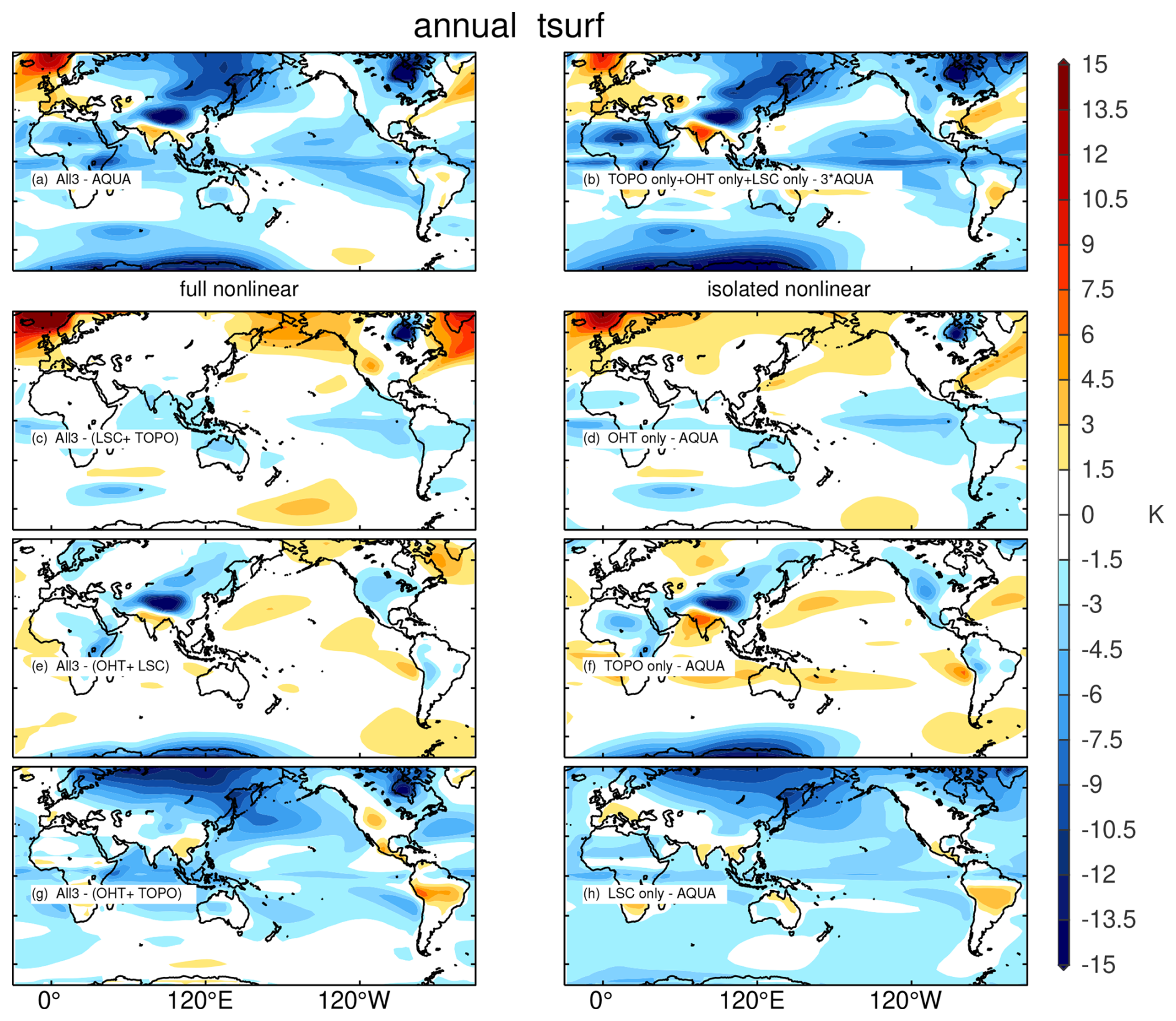
Figure 13 As in Fig. 6 but for surface temperature. The contour interval is 1 K.

OHT also contributes to the NH vs. SH asymmetry in storm tracks (Fig. 9a3, b3) primarily through the surface input term: OHT preferentially fluxes heat to the extratropical NH more than the extratropical SH, which necessitates a reduction in atmospheric heat transport, mostly in the NH. The bulk of this reduction is accomplished via transient eddies. However, the stationary eddy term is also involved in the net MSE flux response, as the zonal component of realistic OHT strengthens stationary waves preferentially in the NH, and so this also necessitates a reduction in transient eddies in the NH relative to the SH. It is worth noting that further intensifying the OHT into the North Atlantic actually weakens the stationary eddy term (Fig. 11a2, b2), and so the details of the OHT pattern matter when considering the changes in stationary eddies. Finally, the TOA longwave term acts as a negative feedback on the effects from stationary eddies and surface energy input: OHT preferentially warms the NH which leads to more longwave cooling to space; this increase in NH longwave increases the energy deficit in the NH extratropics and thus partially mitigates the reduction in NH TE that would otherwise be required (Fig. 9a3, b3). This warming of the NH by OHT is consistent with previous work (Feulner et al., 2013; Kang et al., 2015).

Topography dampens storm tracks both over the Tibetan Plateau and the Southern Ocean (Fig. 6e, f), however the effect is stronger by more than a factor of two when topography is added to an aquaplanet as compared to added last. Furthermore, topography strengthens storm tracks in the North Pacific and North Atlantic more strongly when topography is added onto an aquaplanet. This effect on NH ocean storm tracks can be qualitatively explained by the impact of topography on surface temperature (Fig. 13e, f), with regional subpolar cooling leading to locally stronger storm tracks. The weakening of Southern Ocean storm tracks when topography is imposed on an aquaplanet is consistent with Patterson et al. (2020) and Singh et al. (2016), and potential causes are discussed in detail in these papers. This Southern Ocean response can also be interpreted as an equatorward shift of the storm track, and adding Antarctic topography onto an aquaplanet leads to an equatorward shift of the jet (Fig. 14f).

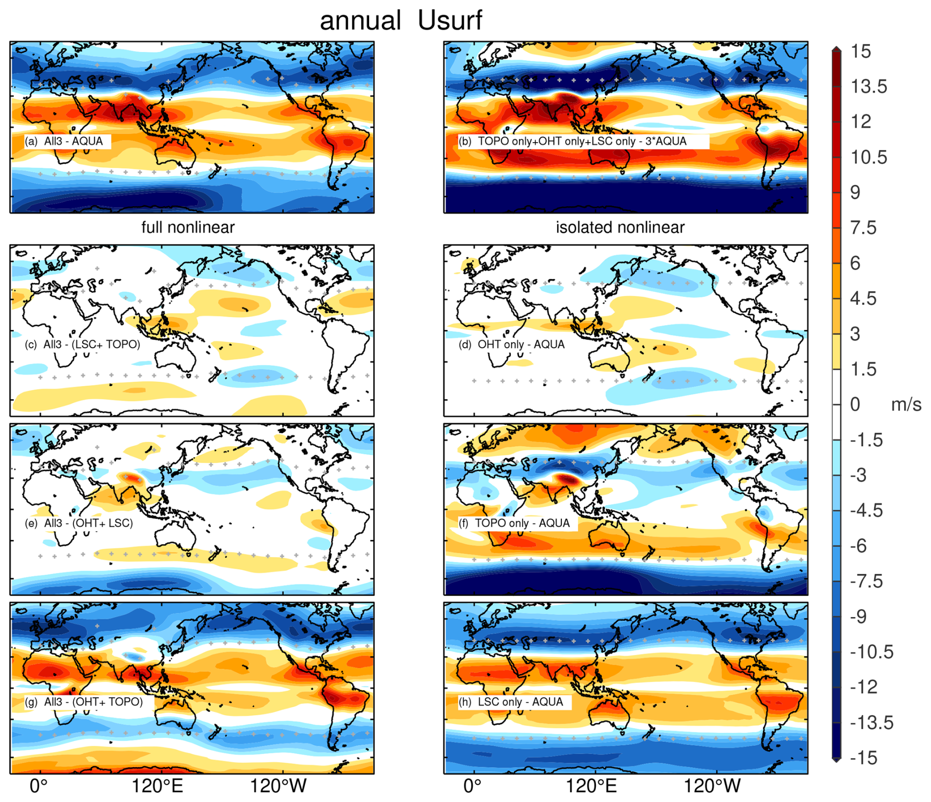
Figure 14 As in Fig. 6 but for zonal wind at the lowest atmospheric model level. The contour interval is 1.5 m s⁻¹. Gray stars indicate the climatological jet maximum in (left) All3 and (right) AQUA.

The weakening of storm tracks directly over the Tibetan Plateau can be interpreted as a local response of the form drag and friction. This response is less pronounced when topography is added to a configuration that already has land–sea contrast because the land–sea contrast leads to weaker baseline near-surface winds over Eurasia, while it is more pronounced when topography is added to an aquaplanet because of the stronger baseline near-surface winds (Fig. 14e, f).

Topography has the weakest effect of any of these three surface inhomogeneities on the NH vs. SH asymmetry in storm tracks (Fig. 9a2, b2), though its effect is more pronounced for 2–8 d TKE definition (Fig. 7). Flattening topography leads to a weakening of the stationary eddy term, however it does not zero it out as it does in the simulations of Shaw et al. (2022). In MiMA, land–sea contrast and OHT force stationary eddies even without topography.

Land-sea contrast weakens the storm tracks over Eurasia and North America when added to an aquaplanet (Fig. 6h) or when added to a configuration that already has the other two (Fig. 6g). Over the Southern Ocean, land–sea contrast weakens the storm track primarily when added to an aquaplanet; this sensitivity to the background state of the Southern Ocean response to land–sea contrast is similar to the effect seen in response to topography (Fig. 6e, f), and may have a similar explanation (compare Fig. 14e, f to g, h), though future work is needed to understand the details. Over the North Atlantic and North Pacific, land–sea contrast weakens storm tracks at subpolar latitudes but strengthens them in mid-latitudes. This mid-latitude strengthening is consistent with the effect described by Brayshaw et al. (2009): cold conditions over Eastern North America and Asia intensify the downstream storm track (Fig. 13g, h). The weakening of the subpolar storm track over the North Atlantic is more pronounced when considering the full nonlinear response, while the weakening over Eurasia is more pronounced in the isolated nonlinear response. These effects likely are related to the surface temperature response, and specifically the local meridional temperature gradient, in these regions (Fig. 13g, h): the temperature gradient in full nonlinear (Fig. 13g) is more pronounced over Eurasia and less pronounced in the North Atlantic as compared to isolated nonlinear (Fig. 13h).

Land-sea contrast is the most important factor for the SH vs. NH asymmetry in storm track strength when using the MSE perspective (Fig. 9a4, b4) or the full nonlinear TKE perspective (Fig. 7; though notably OHT is more important for the isolated nonlinear TKE perspective in Fig. 7). The MSE budget reveals two causes for this: land–sea contrast preferentially enhances the stationary eddy MSE flux in the NH, and land–sea contrast also acts to cool the NH more than the SH, which leads to less TOA OLR in the NH. This reduction in OLR and increase in stationary eddies lead to a reduction in the transient MSE flux that is needed for an energetic equilibrium.

8 Discussion and outlook

We now discuss our results in the context of previous work.

8.1 Comparison to previous results on hemispheric asymmetry

Our results agree with previous work in terms of the importance of topography and OHT on the hemispheric asymmetry of the storm tracks (Manabe and Terpstra, 1974; Shaw et al., 2022, cf. Figs. 7, 9). Interestingly, in MiMA land–sea contrast is the most important of the three surface inhomogeneities for most storm track metrics, which clearly contrasts with the conclusions of Manabe and Terpstra (1974) and Shaw et al. (2022). There are a few possible reasons for this difference.

1. The albedo in MiMA is specified to be similar to the time mean state of CERES, however, there are no radiatively active clouds. In contrast, the ECHAM6 simulations of Shaw et al. (2022) have a full cloud scheme with smaller biases as compared to many other CMIP6 generation models (Mauritsen et al., 2019), however, there are nonetheless albedo biases in midlatitudes (Fig. 2). We have performed a MiMA experiment designed to isolate the role of this albedo bias by mimicking the albedo bias in ECHAM6, and it indicates that this bias is not critical for storm track climatology in the hemispheric mean, though it does have regional impacts (Figs. 11c and 12c). More generally, MiMA does not have a realistic land surface (rather, the heat capacity, surface roughness, and moisture availability are modified to mimic land) and therefore might misrepresent the role of LSC.

2. Outgoing longwave radiation at TOA in MiMA is essentially dictated by surface temperatures, however, longwave radiation on Earth is modulated by clouds. We expect that adding longwave cloud radiative effects would weaken the extremely tight relationship between surface temperature asymmetries and TOA OLR asymmetries (r = 0.99, Fig. 10c), and hence would change the sensitivity of the TOA OLR term to surface inhomogeneities. Nonetheless, the NH is warmer than the SH in observations and comprehensive models (Feulner et al., 2013; Kang et al., 2015), and so the asymmetry in ALL3 is a real effect.

3. MiMA shows an overly strong asymmetry in the transient MSE flux (34 %; Fig. 9) as compared to ECHAM and ERA5 (23 %), likely associated with an overly strong asymmetry in the stationary eddy term in MiMA. There is no such bias in ECHAM (compare Figs. 2 and S2 of Shaw et al., 2022 to Fig. 9b1 red term for All3 in MiMA). The bias in MiMA is primarily due to weak stationary eddies in the SH (Table 2). SH stationary eddies in CMIP are also highly biased across models, and the stationary eddies in MiMA fall within the intermodel range (Garfinkel et al., 2020a). Nonetheless, future work should revisit the role of land–sea contrast for the SH vs. NH asymmetries in a configuration of MiMA with more realistic stationary eddies in the SH, as the importance of LSC in MiMA might be a consequence of biases in its mean state.

The net effect is that while the TOA term responds to surface inhomogeneities in a qualitatively similar manner in both the ECHAM6 simulations of Shaw et al. (2022) and in the MiMA simulations in this paper, the TOA term is more sensitive to surface inhomogeneities in MiMA. The specification of other surface inhomogeneities differs between MiMA and ECHAM6 (e.g., the treatment of land), and this could also indirectly affect the response to land–sea contrast given the strong non-additivity of storm tracks.

Cloud parameterizations are still a sore spot in many models (Duffy et al., 2026), and the results in both papers should be revisited as cloud parameterizations are improved in CMIP class models. More generally, differences in cloud responses across models have been shown to be sufficient to change the sign of the response of, say, SH storm tracks to lowering of Antarctic topography (Justino et al., 2014; Singh et al., 2016), and so bias and errors associated with cloud parameterizations are a key source of uncertainty in conclusions that can be drawn from the current generation of models.

8.2 Comparison to previous work on regional storm tracks

Brayshaw et al. (2009), Brayshaw et al. (2011), and Saulière et al. (2012) find that all three surface inhomogeneities act to localize storm tracks in the North Pacific and North Atlantic basin, in agreement with our results. These studies further documented non-additivity in the response to each of these inhomogeneities. For example, the land–sea contrast associated with the North American continent shapes the North Atlantic storm track more strongly when the orography is included than when it is absent (Brayshaw et al., 2009). In contrast, our experiment adding land–sea contrast last leads to a weakening of the subpolar North Atlantic storm track, while adding it onto an aquaplanet allows for a strong localized North Atlantic storm track (Fig. 6h). We relate this response in the North Atlantic sector to differences in the subpolar surface temperature response and its impact on the local meridional temperature gradient (Fig. 13g, h): Greenland cools when land–sea contrast is added to an aquaplanet (Fig. 13h), however it does not cool when land–sea contrast is added onto a configuration that already has topography (Fig. 13g). Brayshaw et al. (2009) did not include Greenland in their simulations, however Greenland is known to influence storm development (Junge et al., 2005; Jung and Rhines, 2007; Andernach et al., 2025). Future work should isolate its role for climatological North Atlantic storm track strength and location.

The zonal structure in the SH storm track is particularly pronounced in austral winter, and Inatsu and Hoskins (2004), Singh et al. (2016), and Patterson et al. (2020) focus on causes of this asymmetry. Inatsu and Hoskins (2004) argue that zonal structure in SSTs is responsible for most of the large-scale storm track structure in the SH midlatitudes, while Patterson et al. (2020) pinpoint the crucial role of Antarctic topography. Figure S7 isolates the role of each building block in JJAS, and demonstrates that both orography and OHT strengthen storm tracks in the Indian Ocean sector. However, topography appears to be slightly more important for this localization (Fig. S7e, f vs. Fig. S7c, d). The net effect is that the relatively strong SH storm track in the Indian Ocean sector in ALL3 is mostly due to the fact that East Antarctica has higher topography relatively close to the continental edge (consistent with Patterson et al., 2020, who additionally diagnose the relevant dynamics behind this effect), but with east-west gradients in OHT also playing a role (Inatsu and Hoskins, 2004). This effect is much stronger at T85 resolution than at T42 (Fig. 1), which is not surprising given the nature of SH topography.

8.3 Implications for CMIP class models

While all CMIP-class models used for climate projections have realistic topography and continental distribution, the strength of the ocean heat transport into the North Atlantic differs by more than a factor of two (Roberts et al., 2020), even if attention is restricted to HighResMIP models. Heat transport is also too weak in nearly all coarse resolution models, though some higher resolution models are relatively better performing. Southern Ocean sea surface temperature biases are also prevalent and generally not improved at high resolution (Moreno-Chamarro et al., 2022, 2025), and while some of the biases can be linked to biases in clouds or sea ice, this biased climatology affects storm track strength (Moreno-Chamarro et al., 2025). These mean state biases contribute to intermodel spread in future climate projections (Jackson et al., 2023), and there are large observational uncertainties in surface flux trends in the CERES era (Loeb et al., 2022; Mayer et al., 2024).

In our experiments, a relatively small change to regional OHT (well within observational uncertainty) causes large changes in regional storm track strength (Fig. 12a), specifically localized strengthening (Wenta et al., 2024) but hemispheric weakening (cf. Fig. 3k, l). These changes in regional OHT also influence stationary wave strength, and so it is oversimplified and incorrect to predict the changes in storm track strength as a simple compensation to the altered OHT (Fig. 11a), though other modeling studies have observed a higher degree of compensation than we find in response to idealized topography or Last Glacial Maximum conditions (Donohoe et al., 2020; Cox et al., 2022). Either way, the emerging discrepancy in storm track trends between CMIP and observations is likely linked to a misrepresentation of sea surface temperature trends in models and subsequent stationary Rossby wavetrains that spread biases remotely (Kang et al., 2024a), due to the strong linkage between surface energy input and stationary eddy terms. Finally, because the net response to any surface inhomogeneity is dependent on the background state set up by the other inhomogeneities (as we demonstrate throughout this paper), differences in the background state across models due to differing biases in OHT or clouds can then lead to spread in how topography and land–sea contrast affect storm tracks. The net effect is that our study helps us understand why it is so difficult to remove lingering storm track biases from CMIP class models, while pinpointing physical processes that influence their behavior.

8.4 Future work

We used two distinct metrics to track storm tracks: moist static energy fluxes and transient kinetic energy. In many aspects the two metrics gave similar answers, however the role of OHT is somewhat larger for transient kinetic energy (Figs. 7 and 9). While TKE is largest in the upper troposphere, transient MSE fluxes are influenced by moisture and therefore peak in the lower troposphere (Figs. S8 and S9). This might explain some of the disagreement regarding the impact of the different inhomogeneities for the NH-SH asymmetry. More generally, Figure S8 and S9 reveal non-additivity in the latitude vs. height distribution of TKE. Future work should consider the vertical structure of storm track and temperature changes to help understand the forcing mechanisms behind non-additivity, and could also consider a Lagrangian perspective on storm tracks. Future work could explore the relative roles of dry vs. moist processes for the results found in this paper, and also explore why some models show stronger compensation between stationary eddies, the mean meridional circulation, and transient eddies than we find here (Donohoe et al., 2020; Cox et al., 2022, 2024).

An assumption throughout this paper is that each of the three surface inhomogeneities is independent of the rest. This is because our goal is to represent each of the three surface inhomogeneities as closely as possible to current Earth-like conditions. Nonetheless, the ocean circulation would be drastically different if the current configuration of continents were changed or if topography was flattened (Singh et al., 2016), and MiMA's “water mountains” (i.e., topography without land–sea contrast) are highly idealized. If we allowed the ocean circulation to change, we expect that non-additivity would be even more pronounced. Future work should explore this possibility via coupling to a full ocean. Finally, future work should focus on how these localized storm tracks change in response to increased CO₂ by repeating the simulations here, but with elevated CO₂ concentrations.

Appendix A: Albedo

The revised formulation is

$$\begin{array}{}\text{(A1)}& \begin{array}{rl}& {\text{albedo}}_{\text{part 1}}=\mathrm{0.18}+{\displaystyle \frac{\mathrm{0.64}-\mathrm{0.18}}{\mathrm{2}}}\\ & \left(\mathrm{1}+\tanh \left({\displaystyle \frac{\mathit{\varphi }-\mathrm{56}}{\mathrm{24}}}\right)\right)+{\displaystyle \frac{\mathrm{0.72}-\mathrm{0.18}}{\mathrm{2}}}\left(\mathrm{1}-\tanh \left({\displaystyle \frac{\mathit{\varphi }+\mathrm{55}}{\mathrm{20}}}\right)\right),\end{array}\end{array}$$

and the resulting profile is shown in blue in Fig. 2. To better capture the observed plateau in albedo in midlatitudes, we then add a dipole perturbation of the form

$$\begin{array}{}\text{(A2)}& \begin{array}{rl}{\text{albedo}}_{\mathrm{final}}& ={\text{albedo}}_{\mathrm{part}\mathrm{1}}+\mathrm{0.1}\exp \left(-{\displaystyle \frac{(\mathit{\varphi }+\mathrm{53}{)}^{\mathrm{2}}}{\mathrm{200}}}\right)\\ & \sin \left(\mathrm{5}(\mathit{\varphi }+\mathrm{50})\right)-\mathrm{0.1}\exp \left(-{\displaystyle \frac{(\mathit{\varphi }-\mathrm{59}{)}^{\mathrm{2}}}{\mathrm{200}}}\right)\\ & \sin \left(\mathrm{5}(\mathit{\varphi }-\mathrm{55})\right),\end{array}\end{array}$$

The increased albedo over Australia, the Gobi Desert, and the Sahara Desert are unchanged from Garfinkel et al. (2020a). We additionally increase the albedo over Greenland (305–335° E, 66–81° N) to 0.68. The resulting albedo is shown in Fig. 2c, while the albedo profile from White et al. (2021a) is shown in Fig. 2b. Note that the hemispherically averaged albedo in all configurations (including the original specification in red on Fig. 2) is similar between the SH and NH. The net effect is that the hemispheric area-weighted average albedo in the updated configuration is 0.2962 in the NH and 0.3010 in the SH, with the SH vs. NH asymmetry closely matching that in CERES (0.3094 in the NH and 0.3173 in the SH). The mean albedo is slightly lower than in CERES due to the lower tropical albedo (0.18 vs. 0.22), and this profile is shown in pink in Fig. 2. Note that the lower bound on albedo (which in practice is the tropical albedo) is set to 0.18. This choice is due to our desire to not change the globally averaged area-weighted albedo from the red curve. This updated albedo profile leads to a strengthening of near-surface winds as compared to the White et al. (2021a) configuration (not shown), and so we increase surface roughness over ocean to 5.5 × 10⁻⁴ m from 3.21 × 10⁻⁵ m for all experiments in this paper. Globally averaged temperature is similar in all MiMA configurations (by design). In Sect. 5 we assess sensitivity of the storm tracks to the value of albedo over the North Pacific and North Atlantic (Fig. 2d).

Appendix B: Ocean heat flux

We increase heat uptake in the Southern Ocean,

$$\begin{array}{}\text{(B1)}& \mathrm{\nabla }\cdot \mathbf{F}=-\mathrm{3.2105}\times A\times \exp \left(-{\displaystyle \frac{{\left(\mathit{\varphi }+\mathrm{48}\mathit{°}\right)}^{\mathrm{2}}}{\mathrm{2}\times \mathrm{25}\mathit{°}}}\right)\left(-\mathrm{30}\mathit{°}\ge \mathit{\varphi }\ge -\mathrm{61}\mathit{°}\right)\end{array}$$

with an opposing change in the North Atlantic:

$$\begin{array}{rl}\mathrm{\nabla }\cdot \mathbf{F}& =\mathrm{11.9}\times A\times \left(\mathrm{1}-{\left({\displaystyle \frac{\mathit{\varphi }-\mathrm{68}\mathit{°}}{\mathrm{8}\mathit{°}}}\right)}^{\mathrm{4}}\right)\times \cos \left(\mathrm{6}(\mathit{\lambda }-\mathrm{2}\mathit{°})\right);\\ & (\mathrm{60}\mathit{°}\le \mathit{\varphi }\le \mathrm{76}\mathit{°};\mathit{\lambda }\le \mathrm{17}\mathit{°}\text{or}\mathit{\lambda }\ge \mathrm{347}\mathit{°})\end{array}$$

$${\displaystyle }\begin{array}{rl}\mathrm{\nabla }\cdot \mathbf{F}& =\mathrm{16}\times A\times \exp \left(-{\displaystyle \frac{(\mathit{\lambda }-\mathrm{2}\mathit{\varphi }-\mathrm{220}\mathit{°}{)}^{\mathrm{2}}}{\mathrm{2}\times \mathrm{100}\mathit{°}}}\right)\\ & \times \exp \left(-{\displaystyle \frac{{\left(\mathit{\lambda }+\mathit{\varphi }-\mathrm{335}\mathit{°}\right)}^{\mathrm{2}}}{\mathrm{2}\times \mathrm{625}\mathit{°}}}\right);\\ & \left(\mathrm{275}\mathit{°}\le \mathit{\lambda }\le \mathrm{335}\mathit{°},\mathrm{10}\mathit{°}\le \mathit{\varphi }\le \mathrm{52}\mathit{°}\right)\\ \mathrm{\nabla }\cdot \mathbf{F}& =\mathrm{21}\times A\times \left(\mathrm{1}-{\left({\displaystyle \frac{\mathit{\varphi }-\mathrm{76}\mathit{°}}{\mathrm{6.5}\mathit{°}}}\right)}^{\mathrm{4}}\right)\times \cos \left(\mathrm{2}(\mathit{\lambda }-\mathrm{30}\mathit{°})\right);\\ & \left(-\mathrm{15}\mathit{°}\le \mathit{\lambda }\le \mathrm{75}\mathit{°},\mathrm{71}\mathit{°}\le \mathit{\varphi }\le \mathrm{83}\mathit{°}\right)\end{array}$$

where ∇⋅F is the ocean energy flux divergence, and F the implied ocean heat transport. The global average of these perturbations is zero.

At steady state, ∇⋅F equals the surface energy balance. The parameter A represents oceanic interhemispheric heat transport in the Atlantic sector. Setting A equal to 2.1 W m⁻² leads to a more realistic net heat transport to the NH, and the net effect of this perturbation with A = 2.1 W m⁻² is shown in Fig. 3c, while the configuration from White et al. (2021a) with A = 0 W m⁻² is in Fig. 3b.