The moisture mode-to-gravity wave spectrum as a framework to define tropical weather systems

While mid-latitude weather is commonly described in terms of discrete “weather systems”, such as cyclones and fronts, an equivalent framework is less established in the tropics due to the wide range of relevant scales. Instead, tropical weather is often analysed either in Lagrangian terms, through the tracking of mesoscale convective systems, or via spectral decomposition into planetary-scale wave-like disturbances. Here, we use both spectral analysis and Lagrangian object tracking to develop a novel framework for analysing tropical weather systems. We apply recent theoretical advances to classify convectively coupled tropical motions into three types based on their zonal phase speed: moisture modes, inertio-gravity waves, and mixed systems. We show that, consistent with theory, the observed ratio of low-level temperature to moisture anomalies increases with the system’s phase speed, although moisture variations may not be negligible for inertio-gravity waves. Moisture modes and mixed systems show distinct dynamical structures near and off the equator, while inertio-gravity waves are less clearly differentiated. These characteristics are broadly consistent across the tropics, with some regional variations. We find that moisture modes account for up to 75 % of extreme rainfall events along climatological moist margins, whereas mixed systems dominate in the intertropical convergence zone. Our tropical weather systems framework offers a new way to link large-scale tropical dynamics with precipitation.

1 Introduction

The mean climate state at any location is the aggregate effect of day-to-day variations. For rainfall, in particular, this long-term average is contributed by discrete weather systems. In the mid- to high-latitude regions, there exists a consensus among the research community and the operational meteorological agencies of what constitutes a synoptic-scale weather system. They include surface features, such as fronts (Hewson, 1998; Berry et al., 2011) and cyclones (Murray and Simmonds, 1991; Wernli and Schwierz, 2006), and some mid- to upper-tropospheric flow objects, like potential vorticity (PV) cutoffs and streamers (Wernli and Sprenger, 2007) and warm conveyor belts (WCBs; Madonna et al., 2014) (see also Dowdy and Catto, 2017; Sprenger et al., 2017; Jin et al., 2024). Meanwhile, besides tropical cyclones (TCs) and tropical lows or depressions, there is no consensus on how to define analogous rain-bearing tropical weather systems.

A key challenge is the range of spatial scales on which one may define tropical weather systems. One approach is to focus on thunderstorms and the associated mesoscale convective systems (MCSs; see e.g., Schumacher and Rasmussen, 2020) using object tracking. Alternatively, a complementary view applies spectral analysis to decompose tropical motions into large-scale wave-like disturbances, such as the Madden–Julian oscillation (MJO; Zhang, 2005; Zhang et al., 2020) and equatorial waves (Wheeler and Kiladis, 1999; Kiladis et al., 2009). The MCS point of view examines weather from an object-based perspective and deals with tangible weather elements, like rainfall and clouds, but less with the underlying dynamics. For example, around a single TC, there are sometimes multiple clusters of MCS “objects”, even though they are most likely all under the dynamical influence of the TC. On the other hand, the equatorial wave perspective highlights the dynamics responsible for the rainfall, but views them from an Eulerian point of view. A case of twin cyclonic vortices symmetric about the equator, for example, may be seen through equatorial wave theory as part of the westward propagating n=1 equatorial Rossby (ER) wave (see e.g., Kiladis and Wheeler, 1995), but the trajectories of the two cyclones may diverge, or one may outlive the other, and this cannot be fully explained by equatorial wave theory.

The two examples above motivate the current study to explore a new approach of describing dynamical disturbances in the tropics that is more analogous to that used for the mid-latitudes. Conceptually, the approach is to fill the gap between the planetary-scale waves in the “background” and the smaller-scale MCSs with the synoptic-scale tropical weather systems. Here, we introduce an approach that combines the spectral and object tracking perspectives. Recently, Adames (2022) used a scale analysis of the governing equations to identify seven distinct types of tropical motions. They applied a theoretical framework, developed by a number of authors over the past two decades (reviewed in Sect. 2), in which disturbances are distinguished by the role played by moisture in their dynamics. The theory implies that slow-moving disturbances have the strongest coupling to moisture, and they are known as moisture modes. At the other end of the spectrum, disturbances that move rapidly behave like inertio-gravity waves. Motivated by this work, we separate convectively coupled dynamical systems other than TCs into three categories based on their phase speed: slow systems are described as moisture modes, fast systems as inertio-gravity (IG) waves, and those in between, which we call mixed systems. Using this framework, we aim to answer the following questions.

1. What is the observed relative importance of moisture and temperature perturbations in moisture modes, mixed systems, and IG waves?

2. What are the observed dynamic characteristics of moisture modes, mixed systems, and IG waves?

3. What are the rainfall characteristics associated with moisture modes, mixed systems, and IG waves?

The ability to decompose tropical weather into discrete systems has some useful and beneficial applications. For example, model forecasts of a particular type of weather system could be used in combination with the statistics of such weather systems to forecast the likelihood of an extreme event. Gonzalez et al. (2023) showed that such a conditional forecasting method can lead to improved skill for rainfall extremes occurring over the Maritime continent. Another application would be to investigate the changes in tropical rainfall in a warming climate. As emphasised in previous studies (e.g., Chadwick et al., 2013), changes in tropical precipitation under global warming are not as simple as the Clausius-Clapeyron scaling of 7 % increase per 1 K of warming. The weather system framework could allow such changes to be separated into changes in frequency of different system types and changes in their respective contribution to rainfall, as has been done in the extratropics (e.g., Pepler et al., 2021), helping to elucidate the key physical mechanisms at play.

In the next section, we summarise the theoretical framework underlying our separation of tropical weather systems; the moisture mode-to-gravity wave spectrum. In Sect. 3, we explain our methodology of defining weather system types. Section 4 presents the main characteristics of each type of tropical weather system. We explore how these systems affect the occurrences of extreme rainfall events by investigating the rainfall characteristics associated with each of them in Sect. 5. Lastly, we present the summary and discuss the results in Sect. 6.

2 Moisture Mode-to-Gravity Wave Spectrum Theory

Here we introduce the theoretical framework of tropical motions existing on a spectrum between fast inertio-gravity waves and slow moisture modes, each with contrasting propagation and maintenance mechanisms. We begin with the study of Raymond and Fuchs (2007) that sought to explain the complementary control of convective inhibition and lower-tropospheric moisture on convection. They developed an idealised atmospheric model with two distinct unstable modes. The first mode governs the precipitation by modulating the column saturation fraction (i.e., the ratio between column specific humidity and column saturation specific humidity), which they referred to as a moisture mode. The second mode controls convection by altering the convective inhibition just above the boundary layer, and this buoyancy-modulating system was identified as a convectively coupled gravity wave. While buoyancy itself is also affected by moisture anomalies, moisture modes are distinct in that they are present even under weak temperature gradient (WTG; e.g., Sobel and Bretherton, 2000) conditions, with no large-scale buoyancy anomalies. These two distinct modes were also found to move at different speeds, with the moisture mode propagating slower than the convectively coupled gravity wave.

Moisture modes themselves were first described in a modelling study by Sobel et al. (2001). By applying the WTG approximation and adding a prognostic moisture equation to their shallow water model of the tropics, they discovered a mode that owes its existence to horizontal moisture advection. This mode is related to the background horizontal moisture gradient in a manner similar to how the barotropic Rossby wave is related to the background potential vorticity gradient. Later studies suggest that some of the well-known forms of tropical intraseasonal variability, such as the MJO (e.g., Sobel and Maloney, 2013; Adames and Kim, 2016; Monteiro and Sukhatme, 2016; Ahmed, 2021; Suhas et al., 2022; Mayta and Adames Corraliza, 2023), which does not appear in any dry atmosphere models, and the ER wave (e.g., Mayta et al., 2022; Mayta and Adames, 2023; Matthews, 2025), whose observed propagation characteristics are slightly different from what the dry theory suggests, may be moisture modes. The main characteristic of a moisture mode is that it has strong moisture perturbations throughout the lower free troposphere, creating an environment that is supportive of deep convection (Raymond and Fuchs, 2007). Due to their slow propagation, moisture modes are also characterised by WTG balance, as their timescale is long enough to allow the temperature anomalies from latent heat release in deep convection to be smoothed out by gravity waves (see e.g., Adames and Maloney, 2021). This implies that the moisture perturbations associated with moisture modes are more important for their dynamics than the temperature or buoyancy perturbations.

Compared to moisture modes, convectively coupled IG waves have been known far longer, as they appear in the solutions of the “dry” shallow water model of equatorial waves in Matsuno (1966). In the atmosphere, disturbances such as the syntoptic-scale 2 d waves appearing over the Western Pacific in Austral Summer have been identified as IG waves (e.g., Takayabu, 1994a, b). With gravity acting as their main restoring force, IG waves induce significant density or buoyancy variations as they propagate, and these buoyancy anomalies reduce the static stability of the tropospheric column (Haertel and Kiladis, 2004). This can lower the convective inhibition above the boundary layer, making the environment more suitable for deep convection. In short, temperature or buoyancy variations are thought to dominate the coupling of IG waves to convection, while moisture variations are thought to dominate this coupling for moisture modes.

The main distinction in the thermodynamics between moisture modes and IG waves can be summarised as a single parameter (Adames et al., 2019; Adames, 2022),

$$\begin{array}{}\text{(1)}& N_{\text{mode}}\equiv {\displaystyle \frac{C_{\mathrm{p}}T{}^{\prime }}{Lq{}^{\prime }}}\simeq {\displaystyle \frac{s{}^{\prime }}{Lq{}^{\prime }}},\end{array}$$

where C_pT is enthalpy, Lq is latent energy, T is temperature, q is specific humidity, s is dry static energy (DSE; $s=C_{\mathrm{p}}T+gz$), z is geopotential height, and the constants $L=\mathrm{2.5}\times {\mathrm{10}}^{\mathrm{6}}$ J kg⁻¹, C_p=1005 J kg⁻¹ K⁻¹, and g=9.81 m s⁻² refer to latent heat of vaporisation, specific heat of dry air at constant pressure, and gravitational acceleration, respectively. The prime (^′) denotes the magnitude of a perturbation associated with a given weather system. The approximation $C_{\mathrm{p}}T{}^{\prime }\simeq s{}^{\prime }$ is based on the assumption that the perturbation in DSE is dominated by that in enthalpy, rather than by that in geopotential. The approximate form of Eq. (1) is more useful because the numerator and denominator now add up to the moist static energy (MSE; $h=s+Lq$) perturbation. The value of N_mode represents the relative size of moisture and temperature anomalies within a given disturbance. As such, we expect moisture modes to have a small value of N_mode because their moisture perturbations are large, while an IG wave would be expected to have a large value of N_mode because it has a large temperature perturbation, which is tightly related to its DSE perturbation.

Adames et al. (2019) and Adames (2022) further find that N_mode is a fundamental parameter governing the dynamics of the tropical atmosphere, and that it may be related to the phase speed of a propagating tropical weather system. Specifically, Adames (2022) performed a comprehensive scaling of the governing equations to show that N_mode could be written as

$$\begin{array}{rl}& N_{\text{mode}}\equiv max\left({\text{Fr}}_{\mathit{\tau }}^{\mathrm{2}},{\text{Bu}}^{-\mathrm{1}}\right){\displaystyle \frac{\mathrm{1}}{\widehat{\mathit{\alpha }}\left(\mathrm{1}-\widehat{\mathit{\alpha }}\right)}},\\ & {\text{Fr}}_{\mathit{\tau }}\equiv {\displaystyle \frac{c_{\mathrm{p}}}{c}},\text{Bu}\equiv {\left({\displaystyle \frac{L_{\mathrm{d}}}{L_y}}\right)}^{\mathrm{2}},\end{array}$$

where Fr_τ is the Froude number, Bu is the Burger number, $\widehat{\mathit{\alpha }}=\left(\partial Lq/\partial p\right){\left(\partial s/\partial p\right)}^{-\mathrm{1}}$ is the ratio between vertical gradient of latent energy and vertical gradient of DSE, also known as the Chikira (2014) scale, c_p is the phase speed of the system, c is the dry gravity wave speed, L_y is the meridional length scale of the system, $L_{\mathrm{d}}=c/f$ is the Rossby radius of deformation, and f is the planetary vorticity. In the tropics, where f is reasonably small, and for synoptic-scale systems, whose L_y∼1000 km, Bu tends to be large. Therefore, here we assume that ${\text{Fr}}_{\mathit{\tau }}^{\mathrm{2}}>{\text{Bu}}^{-\mathrm{1}}$, which implies a direct relationship between N_mode and the phase speed of a disturbance:

$$\begin{array}{}\text{(2)}& N_{\text{mode}}\approx {\left({\displaystyle \frac{c_{\mathrm{p}}}{c}}\right)}^{\mathrm{2}}{\displaystyle \frac{\mathrm{1}}{\widehat{\mathit{\alpha }}\left(\mathrm{1}-\widehat{\mathit{\alpha }}\right)}}.\end{array}$$

In Appendix A, we sketch a derivation of a slightly different version of Eq. (2) following Adames et al. (2019). The assumption that ${\text{Fr}}_{\mathit{\tau }}^{\mathrm{2}}>{\text{Bu}}^{-\mathrm{1}}$ may breakdown, however, for systems occurring near the subtropical edge regions, where f can no longer be considered small, or for systems with L_y≫1000 km, since Bu⁻¹ becomes larger than ${\text{Fr}}_{\mathit{\tau }}^{\mathrm{2}}$. The extent to which this approximation yields meaningful results is discussed further in Sect. 6.

Combined with Eq. (1), the relation in Eq. (2) tells us that systems with slow propagation will have a small value of N_mode and more dominant moisture perturbations, while fast-moving systems will have a large value of N_mode and more significant temperature perturbations, consistent with what was found in Raymond and Fuchs (2007). Moreover, because c_p is a continuous quantity, this means that N_mode is also continuous, and it implies that moisture modes and convectively coupled gravity waves are not a dichotomy of types of tropical weather system, but rather there exists a spectrum of types of system with moisture modes and IG waves at the opposing ends: a moisture mode-to-gravity wave spectrum. Another implication of this is that a system with a moderate propagating speed will have characteristics that are a mixture of those of a moisture mode and an IG wave: a mixed system. An illustration of this spectrum of systems is shown in Fig. 1.

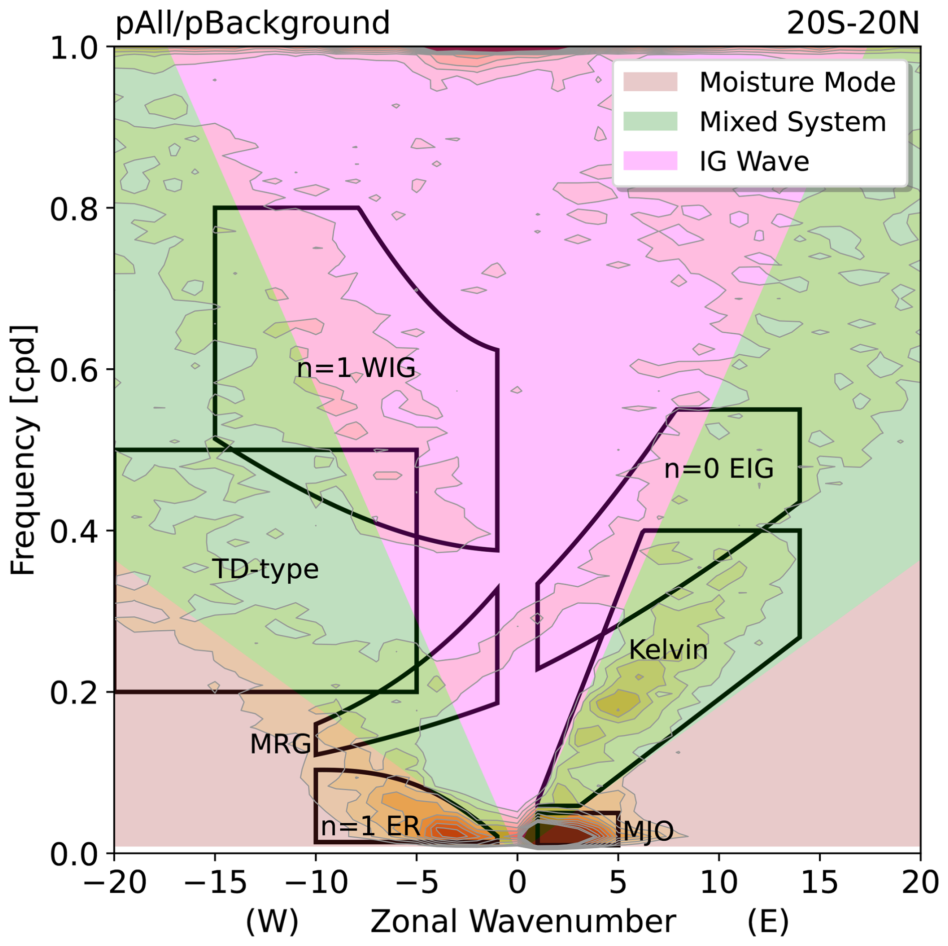
Figure 1 Wavenumber-frequency diagram of the space-time spectra of ISCCP outgoing longwave radiation (OLR) (see Sect. 3 for data description) within 20° S–20° N overlaid with (black lines) some conventional spectral regions of the equatorial waves and the MJO and (coloured polygons) the separation of systems based on the framework described in Sect. 2. The calculation of the space-time spectra follows that of Lubis and Jacobi (2015). Regions of moisture mode, mixed system, and IG wave are determined using Eq. (2) as explained in more detail in Sect. 3.

As noted by Adames (2022), systems with similar thermodynamics (i.e., similar N_mode values) can have different dynamical structures or balances. For example, a moisture mode can exist with a convergent-type low-level dynamics under semigeostrophic balance or with a rotational vortex-like structure under nonlinear balance. Adames (2022) argued that convergent-type moisture modes are more likely near the equator, while rotational-type moisture modes are more likely off the equator. As with moisture modes, mixed systems may also be separated into equatorial convergent-type and off-equatorial rotational-type. Outside of this moisture mode-to-gravity wave spectrum, Adames (2022) identified two other special weather systems in the tropics (cf. Fig. 5 in Adames, 2022), tropical cyclones (TCs), which satisfy gradient wind balance, and moist quasi-geostrophic (QG) systems, which have phase speeds in the range of mixed systems, but have small Rossby numbers and satisfy QG balance, and are typically strongly extratropically influenced. For simplicity, in this paper we limit the scope to focus only on moisture modes, mixed systems, and IG waves, as well as some comparisons to TCs. We find it worth investigating how the separation of the convectively coupled large-scale motion signals in the tropics based on this framework, rather than on the traditional equatorial wave dispersion relations, can help us understand further the complex interactions between large-scale dynamics and moist convective processes.

3 Methods

3.1 Data

As we are investigating the large-scale dynamical systems that are coupled with moist convection, we employ the top-of-atmosphere outgoing longwave radiation (OLR) from the International Satellite Cloud Climatology Project (ISCCP; Zhang and Rossow, 2023) dataset as a reasonable proxy variable for deep convection. To analyse the thermodynamic and dynamic characteristics of tropical weather systems, we make use of the European Centre for Medium-Range Weather Forecasts (ECMWF) Reanalysis v5 (ERA5; Hersbach et al., 2020) dataset. All variables used in this study are listed in Table 1. We use the time period of 1984–2016 for ISCCP and ERA5 variables and, to match the OLR field, all ERA5 variables are spatially regridded, using bilinear interpolation, onto a 1° × 1° grid and temporally resampled from hourly frequency into 3-hourly means.

Table 1 List of variables used in this paper.

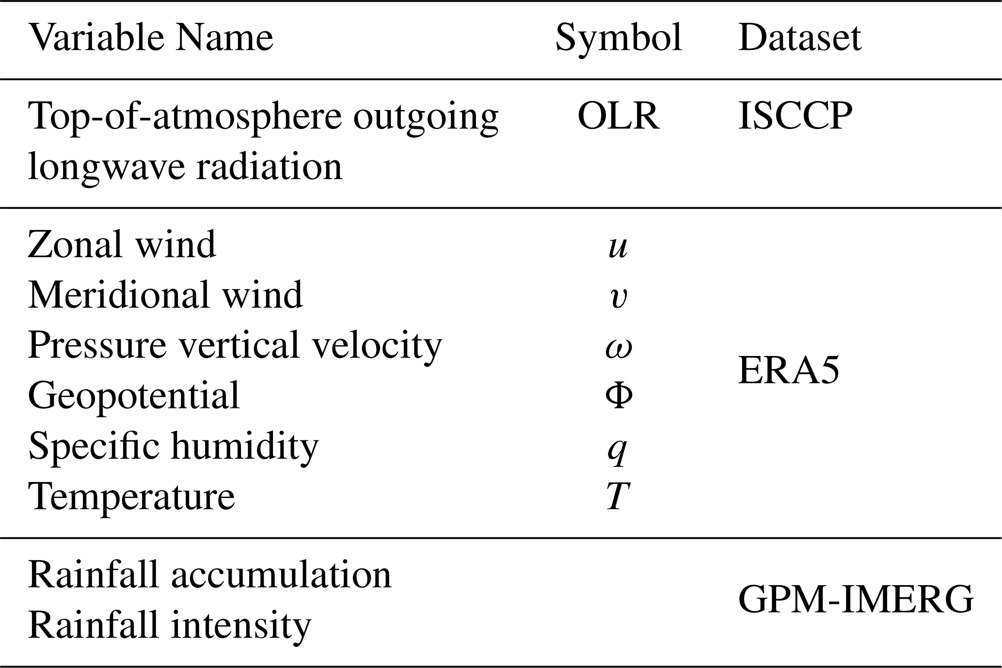
For the extreme rainfall analyses, we compute two variables based on the half-hourly precipitation rate from the Global Precipitation Measurement's (GPM) Integrated Multi-satellite Retrievals for GPM (IMERG; Huffman et al., 2020). Rainfall accumulation is defined as the 3-hourly sum of the half-hourly precipitation rate, whereas rainfall intensity is defined as the 3-hourly mean of only the half-hourly precipitation rate exceeding 0.05 mm h⁻¹. The 3 h time window is chosen to match the temporal resolution of the OLR, while we retain the high spatial resolution of 0.1° × 0.1° to avoid smoothing out any localised extreme rainfall occurrences. For these rainfall variables, the available time period is shorter, from June 2000 to December 2016.

3.2 Separation by Phase Speed

We first separate large-scale convectively coupled signals into moisture modes, mixed systems, and IG waves. This is done by filtering the OLR anomaly field based on phase speed. The anomaly or perturbation of a field is deseasonalised by subtracting the mean and the first four harmonics of the annual cycle, and the diurnal cycle is further removed by subtracting all harmonics with period not greater than 24 h. Following Adames (2022), and using the approximation in Eq. (2), we assume $\widehat{\mathit{\alpha }}=\mathrm{0.9}$ and c=50 m s⁻¹, and make a classification as follows.

• Moisture mode: $N_{\text{mode}}\lesssim {\mathrm{10}}^{-\mathrm{0.5}}$ corresponding to c_p≲9 m s⁻¹

• Mixed system: ${\mathrm{10}}^{-\mathrm{0.5}}\lesssim N_{\text{mode}}\lesssim {\mathrm{10}}^{\mathrm{0.5}}$ corresponding to 9 m s${}^{-\mathrm{1}}\lesssim c_{\mathrm{p}}\lesssim \mathrm{27}$ m s⁻¹

• IG wave: N_mode≳10^0.5 corresponding to c_p≳27 m s⁻¹

This classification is illustrated in Fig. 1. Before the filtering step, we remove the TC signals using a simple method following Aiyyer et al. (2012) based on the International Best Track Archive for Climate Stewardship (IBTrACS; Knapp et al., 2010) dataset. This method uses a Gaussian weighting function to remove anomalies around each TC, where anomalies at the TC centre are reduced to zero and those at distance of 500 km from the centre are reduced by half (see Eq. 1 in Aiyyer et al., 2012 for more details). The remaining field is then used in the filtering following the ranges described above using the 2-D fast Fourier transform (2D-FFT) method (see e.g., Wheeler and Kiladis, 1999; Kiladis et al., 2009; Lubis and Jacobi, 2015). In this method, we employ the preprocessing steps of linearly detrending and tapering both ends of the time series at each grid point, following Wheeler and Kiladis (1999), but without doing any decomposition into symmetric and antisymmetric components. Note also that, for each category, we combine eastward- and westward-propagating signals; this needs to be taken into account when interpreting the composites shown later. Figure 2 shows an example of the results of this separation method for a single snapshot.

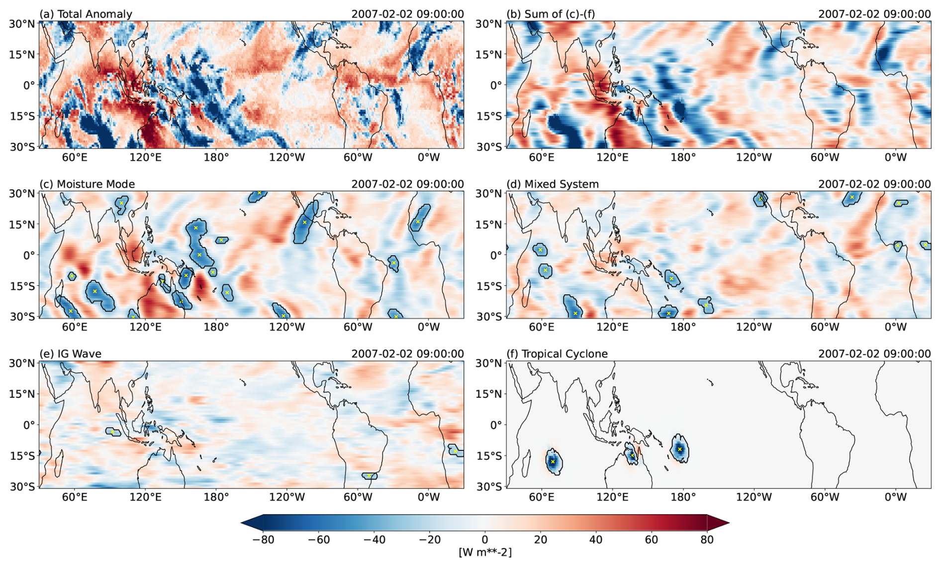
Figure 2 Snapshots of (a) total OLR anomaly, (b) sum of (c)–(f), and OLR anomalies associated with (c) moisture modes, (d) mixed systems, (e) IG waves, and (f) TCs. In (c)–(f), centres of the identified OLR objects are denoted by yellow “x” markers and closed contour lines represent the OLR objects' boundaries as determined by the tobac algorithm (see Sect. 3 for details).

3.3 Object Identification and Tracking

Having filtered the OLR into signals associated with different phase speeds, we then apply a tracking algorithm to identify filtered OLR “objects” as the tropical weather systems. We choose the Tracking and Object-Based Analysis of Clouds (tobac; Heikenfeld et al., 2019; Sokolowsky et al., 2024; tobac Community et al., 2025) algorithm because it has some utilities fit for our analyses here, such as its ability to track objects through a periodic boundary (e.g., periodic longitude in our global domain). As with other object detection methods, tobac defines connected regions around a local minimum/maximum exceeding a certain threshold as an object in a snapshot of a two-dimensional field. In our case, we identify local minima in the filtered OLR anomaly fields (i.e., negative OLR values) as we are only interested in features associated with strong deep convection. We then use tobac to follow the movements of objects through subsequent time steps and determine whether they belong to the same track. For each detected track, we define the instance when the magnitude of the filtered OLR anomaly around the object's centre (defined as the object's centroid) is the greatest as the track's maximum activity, or the lag 0 of the track. More details on the parameter configurations that we use for tobac are described in Appendix B.

3.4 Statistical Composite

To obtain the general characteristics of each tropical weather system, we calculate composite averages of the thermodynamic and dynamic variables. This is done by compositing snapshots of a field in the immediate vicinity of the object's centre for all the detected tracks belonging to a type of system at their respective “lag 0”. We only use “lag 0” to increase the statistical independence of the composited snapshots, since we consider that different objects in a single track are just different life stages of the same physical weather system. Prior to this composite calculation, we separate the tracks based on their maximum activity's locations into equatorial (10° S–10° N), northern hemisphere off-equatorial (10–20° N), and southern hemisphere off-equatorial (20–10° S).

3.5 Extreme Rainfall Probability Change

In addition to this statistical compositing technique, in the extreme rainfall analyses, we also calculate the change in probability of extreme rainfall intensity events. An extreme rainfall intensity event is defined as an instance when rainfall intensity at each grid point exceeds its long-term 99th percentile. We compare the probability of extreme rainfall intensity events at a location for when a tropical weather system is over that location against that for all times, mathematically expressed as

$$\begin{array}{}\text{(3)}& R_P={\displaystyle \frac{P\left(\text{intensity}\ge \mathrm{99}\text{th}\text{pct}|\text{system “X” occurs}\right)}{P\left(\text{intensity}\ge \mathrm{99}\text{th}\text{pct}\right)}}.\end{array}$$

By construction, the denominator in Eq. (3) is 0.01. As with the statistical composites, this quantity R_P is also computed in the immediate vicinity of the object's centre for all the detected tracks belonging to a type of system at their respective “lag 0”.

4 Characteristics and Spatial Distribution of Tropical Weather Systems

In this section, we will present the spatial distribution and general characteristics, both thermodynamic and dynamic, of the tropical weather systems defined in the moisture mode-to-gravity wave spectrum framework.

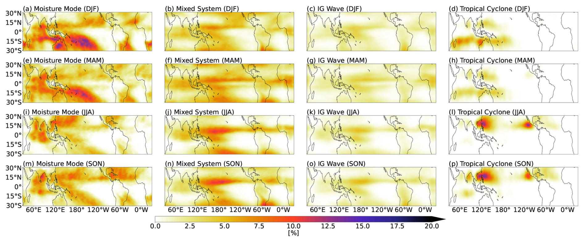
Figure 3 Frequency of occurrence of (a, e, i, m) moisture modes, (b, f, j, n) mixed systems, (c, g, k, o) IG waves, and (d, h, l, p) TCs during (a–d) December–February, (e–h) March–May, (i–l) June–August, and (m–p) September–October. Frequency of occurrence of a system at each grid point is defined as the time frequency of that location being within the system's OLR object boundary.

Figure 3 shows that moisture modes mainly occur along the edges of the deep tropics, around 15° N/S. These regions coincide with the climatological location of the moist margin (see e.g., Mapes et al., 2018; Robinson et al., 2024), where the background horizontal moisture gradient is large. This is thought to be one of the supportive environmental conditions for the maintenance and growth of moisture modes (Mayta and Adames Corraliza, 2024). On the other hand, mixed systems and IG waves are more confined along the intertropical convergence zone (ITCZ), especially over the Pacific and Atlantic, and over some land regions, such as equatorial Africa. We also notice that there are some occurrences of mixed systems, and, to a lesser extent, IG waves, along the northern and southern boundaries of the domain (i.e., 30° N/S). These are likely to be the imprints of extratropical frontal bands and other systems moving with similar propagating speeds: the moist QG systems.

Seasonal variations in track density are consistent with the known seasonal cycle of precipitation in the tropics. For example, along the eastern Pacific during the March–May period, we can see two zonal bands where mixed systems and IG waves mainly occur (Fig. 3f, g), and these bands are also observed in precipitation (the double ITCZ; see e.g., Si et al., 2021). Therefore, from the weather system perspective, we posit that moisture modes might be the building blocks of the South Pacific convergence zone (SPCZ), while mixed systems and IG waves might be the building blocks of the ITCZ.

4.1 Thermodynamic Characteristics

To answer the first question posed in Sect. 1, we create composite averages of the perturbations in latent energy and DSE associated with moisture modes, mixed systems, and IG waves. These are shown as zonal-vertical cross sections in Fig. 4. In Fig. 4a–c, we see that all three types of weather system are associated with an anomalously moist lower free troposphere (red box). This condition creates a supportive environment for deep convection by reducing the dilution of rising parcels through entrainment and detrainment processes (e.g., Ahmed and Neelin, 2018). Furthermore, as expected from the theory, moisture modes have much greater moisture perturbations compared to the other two systems, and these moisture perturbations decrease in magnitude with increasing phase speed. The composites in Fig. 4 show little phase tilt with height, and this is partially a result of the compositing technique, which, as mentioned previously, combines westward- and eastward-moving systems. When these types are separated before compositing (Figs. S1 and S2), we see a clear westward phase tilt for eastward-propagating IG waves, as previously found in Inoue et al. (2020), and a weaker westward tilt of moisture anomalies for eastward-propagating moisture modes.

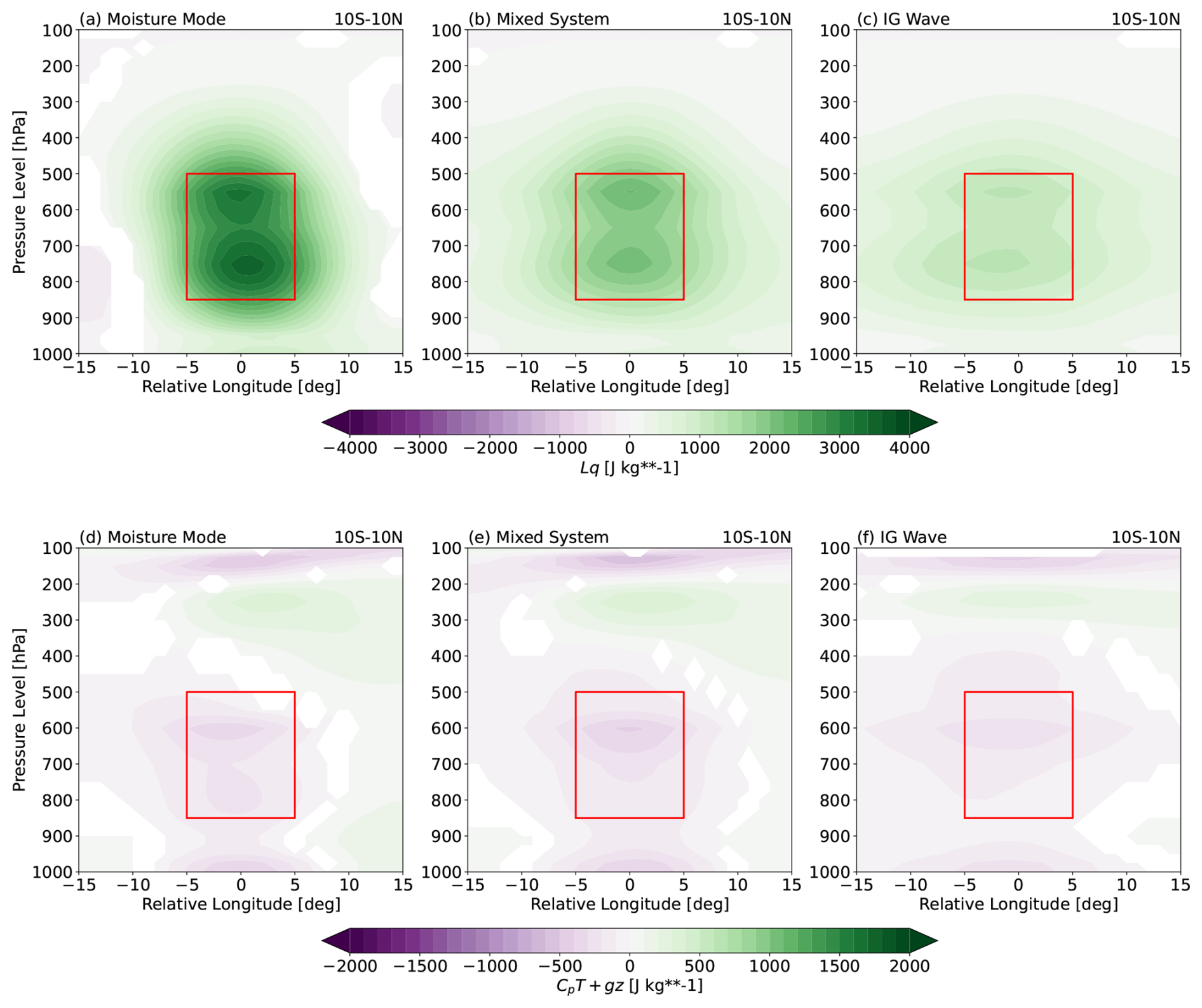
Figure 4 Zonal-vertical cross sections of the composites of (a)–(c) latent energy and (d)–(f) DSE anomalies for (a, d) moisture modes, (b, e) mixed systems, and (c, f) IG waves in the equatorial region. Red box denotes the lower free troposphere, defined as layers between 500 and 850 hPa. Note that the colour bar ranges for (a)–(c) and for (d)–(f) are different. Only statistically significant values at 95 % level are shown, based on the two-tailed Student's t-test.

In the DSE anomaly profiles (Fig. 4d–f), all three systems show negative anomalies just above the boundary layer, which act to lower the convective inhibition in those layers and increase the chance of deep convection. However, we do not see any significant differences in DSE anomaly magnitudes among the three systems. Unlike the Lq perturbation, the DSE anomaly varies only weakly with the system's propagating speed. Hence, although the ratio of DSE to latent energy anomalies (i.e., N_mode) increases with phase speed as hypothesised in Eq. (2), it is mainly due to the change in Lq^′ alone, rather than the changes in both s^′ and Lq^′. This is consistent with Adames (2022), which showed that the numerator in N_mode is independent of any relevant time scale. Moreover, despite the fact that the absolute magnitude of the latent energy anomaly is always larger than that of DSE, we find that the relative role between moisture and temperature does decrease with the system's propagating speed.

Figure 4 only shows the profiles for the weather systems in the equatorial region, but the above results also hold true in general for the systems in the off-equatorial regions (not shown). There are, however, some regional differences among different ocean basins, as exemplified in Fig. 5. Over the Western Pacific region (Fig. 5d–f), the profiles of both thermodynamic variables and the vertical velocity look very similar to those over the tropics in general (Fig. 5a–c). Some noticeable differences are that the latent energy anomaly profiles for all the three systems have slightly larger magnitudes (Fig. 5d) and that they also have slightly stronger anomalous upward motion (Fig. 5f), but the overall profile shapes are very much the same as those in Fig. 5a–c. Over the Eastern Pacific, the moisture perturbations are even larger (Fig. 5g), particularly those in the lower levels for moisture modes. Here, an interesting difference can be seen in the DSE anomaly profiles (Fig. 5h), where there are some positive anomalies near the top of the boundary layer (around 900 hPa) for all three types of systems. We also notice that the anomalous vertical velocity profiles over the Eastern Pacific have somewhat different shapes (Fig. 5i), with a larger vertical velocity amplitude at lower levels; this is particularly visible for moisture modes. These contrasts between the Western and Eastern Pacific might be related to differences in background states, such as sea surface temperature, tropospheric stability, and vertical velocity, of these two regions (see e.g., Back and Bretherton, 2006; Bernardez and Back, 2024).

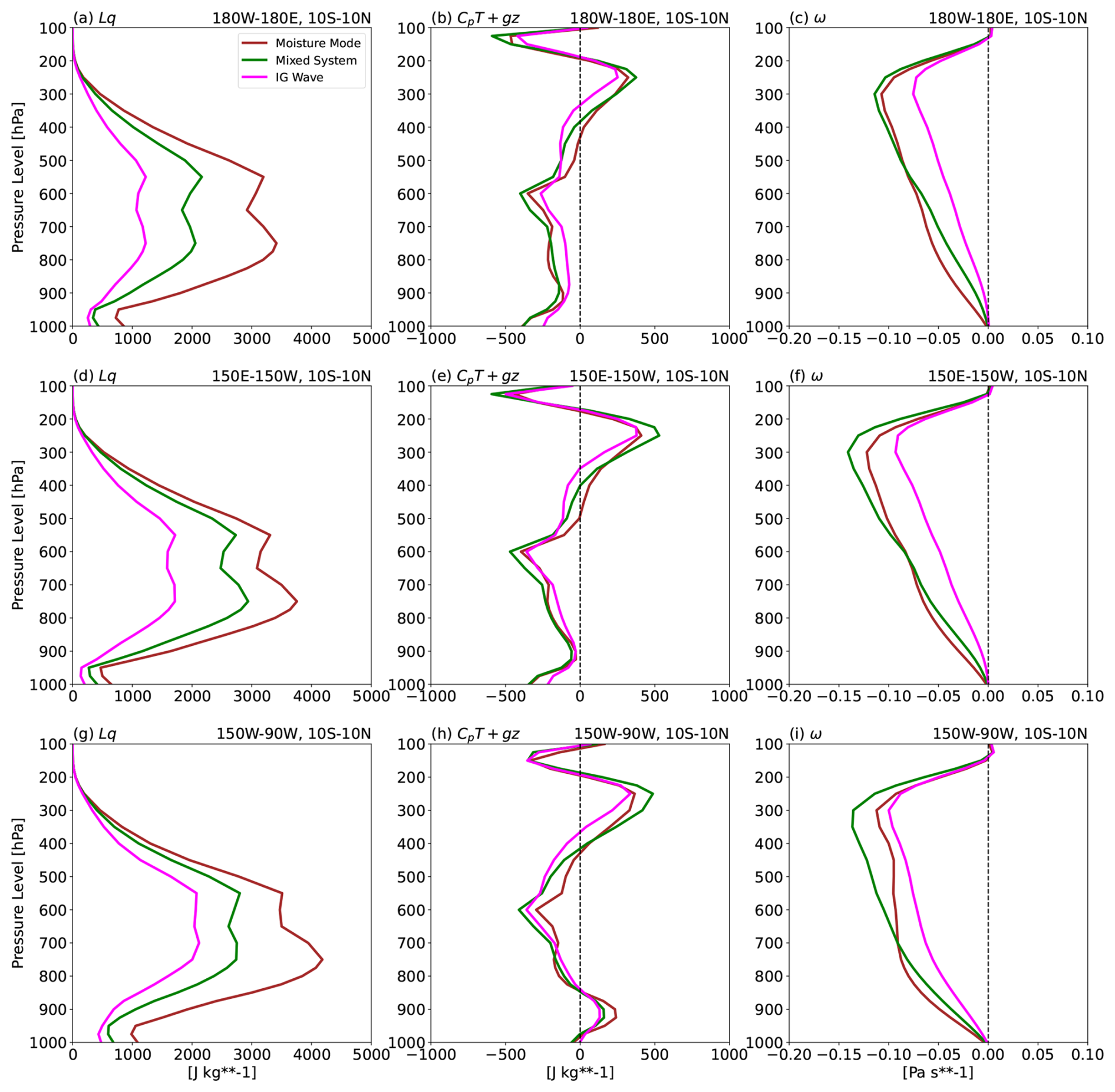
Figure 5 Vertical profiles of the composites of (a, d, g) latent energy, (b, e, h) DSE, and (c, f, i) pressure vertical velocity anomalies for (brown) moisture modes, (green) mixed systems, and (magenta) IG waves in the equatorial region over (a)–(c) the global tropics, (d)–(f) the Western Pacific, and (g)–(i) the Eastern Pacific, averaged over a 4° × 4° box around the object centre. Note that the ranges of the x-axis are different in different columns. Vertical dashed lines in the middle and right columns mark the zero value on the x-axis.

4.2 Dynamic Characteristics

As briefly mentioned in Sect. 2, systems with similar thermodynamics can occur under different dynamical structures or balances. Figure 6 shows composites of dynamical fields for moisture modes, mixed systems, and IG waves occurring in three different latitudinal ranges calculated using the same statistical averaging technique as before, that is, composites are centred around the detected centroids and combine both eastward- and westward-propagating systems. We also show the composites for TCs to compare with, although detailed investigations of the dynamic characteristics of TCs are beyond the scope of this study.

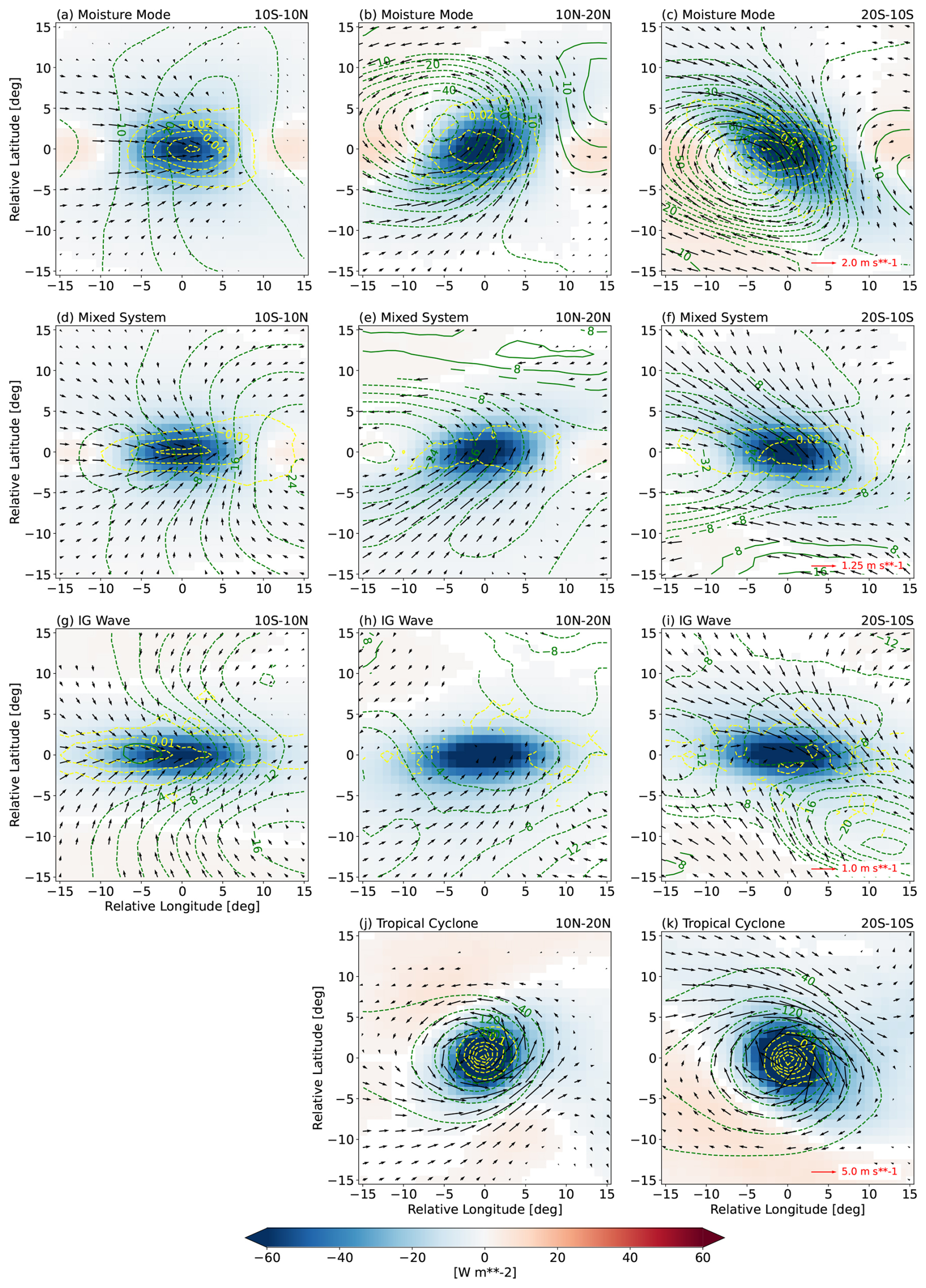
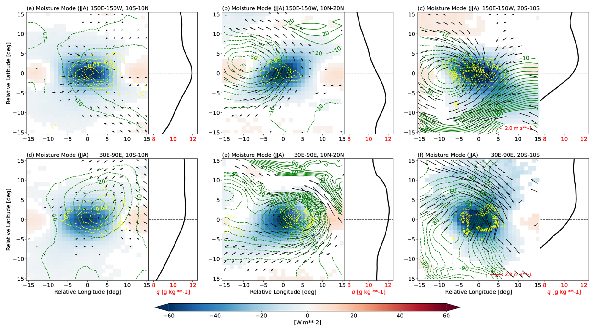
Figure 6 Composites of (shading) OLR, (vectors) 850 hPa horizontal wind (u,v), (green contours) 850 hPa geopotential (Φ), and (yellow contours) 850 hPa vertical velocity (ω) anomaly fields for (a)–(c) moisture modes, (d)–(f) mixed systems, (g)–(i) IG waves, and (j)–(k) TCs in the (a, d, g) equatorial, (b, e, h, j) northern hemisphere off-equatorial, and (c, f, i, k) southern hemisphere off-equatorial regions. Note that the vector length scales, the green contour intervals, and the yellow contour intervals are different in different rows. Units of Φ and ω are m and Pa s⁻¹, respectively. Only statistically significant values at 95 % level are shown, based on the two-tailed Student's t-test.

In the equatorial region, moisture modes are characterised by low-level convergence, mostly due to the confluence of northwesterly and southwesterly anomalous winds (Fig. 6a). The horizontal convergence is accompanied by significant anomalous upward motion in the area of relatively low pressure around the core of the convective region. This low-level dynamical structure very much resembles the theoretical schematic of the equatorial moisture mode in Fig. 5 of Adames (2022), although the strong zonal pressure gradient is not as apparent here in Fig. 6a. This is partially a result of combining both westward- and eastward-propagating signals into a single composite; when the two are separated, the zonal gradient in 850 hPa geopotential is stronger for the eastward-moving moisture mode than the westward-moving one. In the off-equatorial region, moisture modes have a different dynamical configuration, characterised by a vortex rotating in the cyclonic sense (Fig. 6b–c). The anomalous horizontal flow of this vortex is roughly in geostrophic balance, as the wind vectors are almost tangential to the geopotential contour lines. The most interesting feature of the off-equatorial moisture mode, however, is the fact that the convectively active region is not collocated with the low-pressure centre, unlike in the low-level structure of the TC (Fig. 6j–k). Instead, the anomalous OLR and pressure velocity ω are slightly shifted to the east of the vortex centre, where the low-level flow is poleward. This displacement puts the precipitation in a region of positive moisture advection (see also later in Fig. 8), which is argued by Adames and Ming (2018) and Mayta and Adames Corraliza (2024) to be key to the growth and eastward propagation of moisture modes: the moisture-vortex instability (MVI) mechanism.

As with the moisture modes, mixed systems show different dynamical structures near the equator compared to off the equator. The equatorial mixed systems have a strong low-level horizontal confluence, which also coincides with the region of convection and upward motion (Fig. 6d). The zonal pressure gradient is more apparent here, with a minimum in geopotential anomaly located to the east of the convergence, consistent with the schematic in Adames (2022). In the off-equatorial region, mixed systems are also associated with a cyclonic vortex (Fig. 6e–f), but with a weaker vortex strength and a less balanced flow than for moisture modes. The vortex size is also larger in off-equatorial mixed systems and this, again, matches with its theoretical illustration in Adames (2022).

For IG waves, the contrast between equatorial and off-equatorial dynamical structures is less clear than for other system types (Fig. 6g–i). While the low-level anomalous convergence associated with the OLR and upward motion anomalies is evident in the equatorial IG waves (Fig. 6g), the low-level dynamics of the off-equatorial IG waves is dominated only by speed convergence with no clear signals of any rotational flow (Fig. 6h–i).

An important property of a dynamical system is its proximity to balanced flow. For the off-equatorial systems, a relevant balance condition is geostrophic balance. Qualitative comparison of the alignment of the winds and geopotential contours in Fig. 6 suggests that the systems become more unbalanced with increased phase speed. For the equatorial systems, however, the relevant balance condition is nonlinear balance, and this cannot be simply assessed from the winds and geopotential. Instead, we compute a quantity defined as the deviation from nonlinear balance (Bolin, 1955; Charney, 1955; Adames, 2022),

$$\begin{array}{}\text{(4)}& \mathrm{\Sigma }={\mathrm{\nabla }}_h^{\mathrm{2}}\mathrm{\Phi }-f\mathit{\zeta }+u\mathit{\beta }-\mathrm{2}\mathit{k}\cdot \left({\mathbf{\nabla }}_{h}u\times {\mathbf{\nabla }}_{h}v\right)\end{array}$$

where ${\mathrm{\nabla }}_h^{\mathrm{2}}$ is the horizontal Laplacian operator, f is the planetary vorticity, ζ is the relative vorticity, $\mathit{\beta }=\partial f/\partial y$ is the meridional gradient of f, and ∇_h is the horizontal gradient operator. Nonlinear balance is a generalised horizontal balance condition which includes many of the well-known balances, such as the gradient wind, cyclostrophic, and geostrophic balances as special cases (e.g., Bolin, 1955; Charney, 1955). The composites of the low-level Σ anomaly are shown in Fig. 7. It clearly shows that the faster moving systems are more horizontally unbalanced than the slower moving ones, even for those in the equatorial region. Further decomposition suggests that most of the deviation from balance condition comes from the first three terms on the right hand side of Eq. (4), that is, the deviation from geostrophic balance (not shown). This implies that, as for the thermodynamics, there is also a spectrum of dynamics from balanced moisture modes to unbalanced IG waves, in agreement with the theory of Adames (2022).

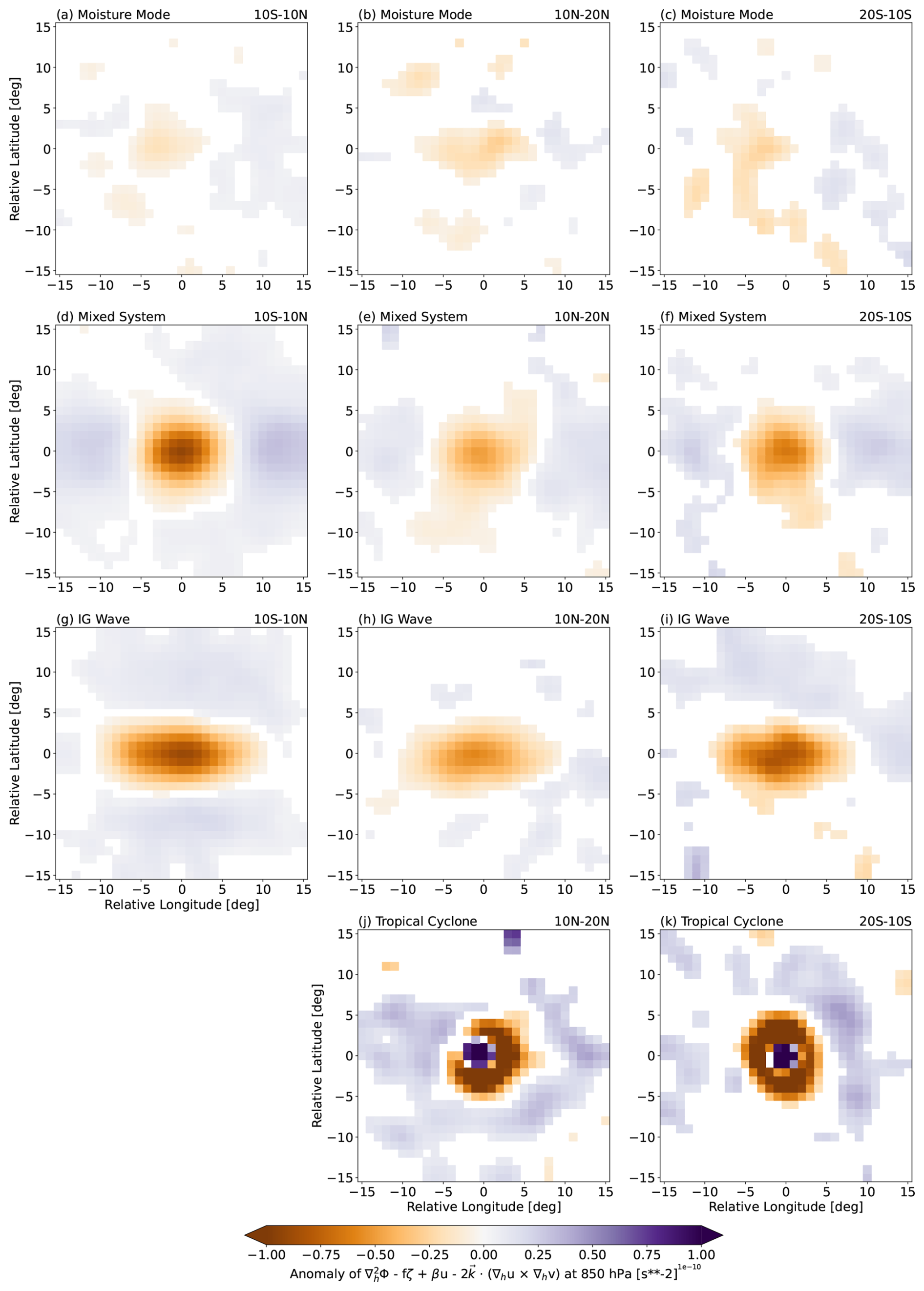
Figure 7 Composites of the anomaly of the deviation from nonlinear balance Σ (see Eq. 4) computed at 850 hPa for (a)–(c) moisture modes, (d)–(f) mixed systems, (g)–(i) IG waves, and (j)–(k) TCs in the (a, d, g) equatorial, (b, e, h, j) northern hemisphere off-equatorial, and (c, f, i, k) southern hemisphere off-equatorial regions. Each instance is smoothed three times using a 1-2-1 filter in both horizontal directions prior to the composite averaging. Only statistically significant values at 95 % level are shown, based on the two-tailed Student's t-test.

As in Sect. 4.1, it is of interest to examine how the dynamic characteristics vary geographically. Here, we present some examples that can also be used to elaborate the MVI mechanism in more detail. Figure 6b–c show that the convectively active region of off-equatorial moisture modes is where the flow of the cyclonic vortex is poleward. This is consistent with MVI theory (Adames and Ming, 2018; Mayta and Adames Corraliza, 2024), which states that moisture build-up owing to positive meridional moisture advection leads to precipitation that is slightly in-phase with the vortex, which can later destabilise the moisture modes by strengthening the vortex through vortex stretching. This is demonstrated specifically for the Western Pacific during June–August in Fig. 8b, c, where the background specific humidity increases towards the equator and the precipitation maximum occurs in the poleward low-level flow. However, moisture modes in the northern hemisphere off-equatorial Indian Ocean at the same time of year show a contrasting low-level dynamical structure (Fig. 8e). In this case, the convectively active region is not to the east, but to the west, of its vortex centre, where the anomalous flow is equatorward. This can be explained by looking at the distribution of the background moisture in that location. During this South Asian monsoon season, the Indian subcontinent to the north is actually more humid than the equatorial Indian Ocean. This reverses the background meridional moisture gradient (line plot in Fig. 8e), allowing an equatorward flow to produce a positive moisture advection. Such a moisture gradient reversal does not happen in the southern hemisphere off-equatorial side of the sector, therefore, the OLR anomaly in Fig. 8f still occurs to the east side of the vortex. We find our results here consistent with the geographical variations of the slow-moving vortical disturbances investigated in Biswas et al. (2026). While the MVI mechanism described so far is useful in elucidating the dynamical structure of the off-equatorial moisture mode, it cannot, however, explain why the convectively active region of the equatorial moisture mode occurs where the background meridional moisture gradient is virtually zero (Fig. 8a, d). While detailed analyses of the maintenance mechanisms of equatorial moisture modes are left to future work, preliminary analysis of the MSE budget (not shown) suggests that zonal advection, rather than meridional advection, may play a greater role for the growth and propagation of equatorial moisture modes than for their off-equatorial counterparts. This is consistent with Adames and Kim (2016) and Wang and Sobel (2022) who also argued that equatorial moisture modes, such as the MJO, grow through different mechanisms which do not require a large local meridional moisture gradient.

Figure 8 As in Fig. 6a–c, but only for moisture modes over (a)–(c) the Western Pacific and (d)–(f) the Indian Ocean during June–August. Line plot to the right of each panel shows the composite of the 850 hPa specific humidity field, averaged zonally across the domain.

5 Impacts on Extreme Rainfall

We associate rainfall with a weather system if it falls within a 1000 km radius of the system centre at any time during its lifetime (see Fig. 9). This method is chosen to also account for rainfall in the vicinity of the systems but outside of their OLR object boundaries. According to this attribution method, the four tropical weather systems studied here, including TCs, are found to be associated altogether with about 60 % of total rainfall received within the global deep tropics (20° S–20° N; Fig. 10). Individual influences of moisture modes and mixed systems are each associated with almost 20 % of total rainfall. Meanwhile, IG waves and TCs individually contribute much less to rainfall in this region, only up to 5 % each, due partly to their less frequent and less widespread occurrences compared to moisture modes and mixed systems (Fig. 3). Besides these individual contributions from the four systems, the “compound” influences of more than one type of system (i.e., occurring at the same location and at the same time) are also significant, about 10 % of total rainfall (not shown), making the “sum” term in Fig. 10a greater than 50 %. If we only consider heavy rainfall as in Fig. 10b, defined as rainfall above an accumulation of 30 mm (3 h)⁻¹, the total contribution from the four systems investigated here increases to almost 80 %, leaving only around 20 %–25 % of unexplained high rainfall events. This indicates that the weather systems defined in this study account for the vast majority of heavy and impactful rain events in the tropics.

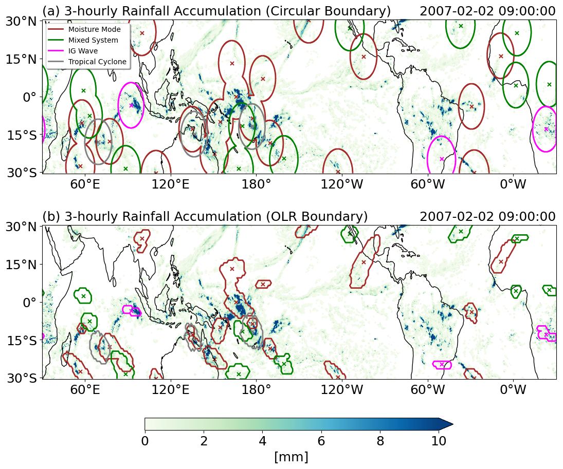
Figure 9 Snapshot of 3-hourly rainfall accumulation overlaid with (a) the 1000 km radius circles around the systems' detected centres and (b) the OLR object boundaries as in Fig. 2.

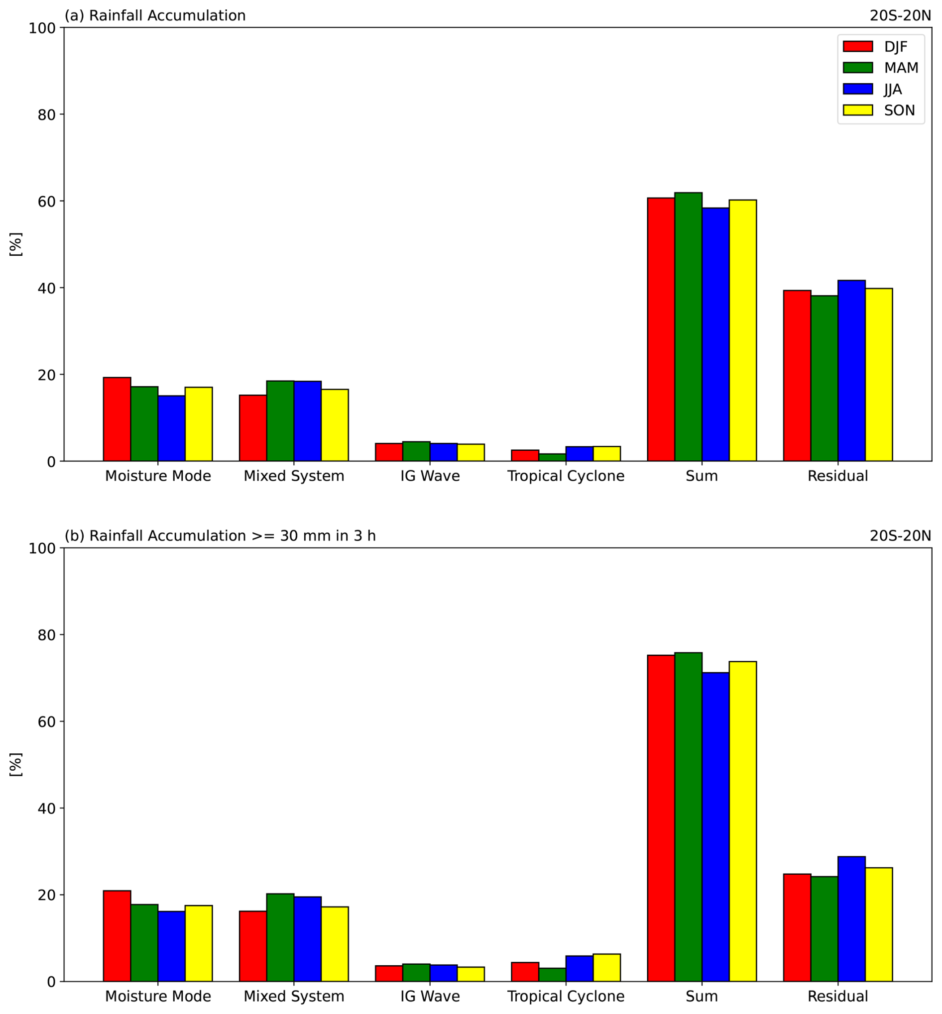
Figure 10 (a) Percentages of seasonal rainfall accumulation within the deep tropics associated with moisture modes, mixed systems, IG waves, and TCs, as well as the sum and the residual. (b) As in (a), but only for rainfall accumulation greater than or equal to 30 mm (3 h)⁻¹. The “sum” term here is the sum of the four individual systems and the “compound” occurrences of more than one type of system at a location (not shown). The “residual” term includes rainfall not associated with any of the four system types.

To further investigate the potential impacts of these weather systems on tropical rainfall, we assess the general characteristics of rainfall associated with each of these systems. In the equatorial region, mean rainfall intensity around the centres of moisture modes, mixed systems, and IG waves at their time of maximum OLR activity can reach 2 mm h⁻¹, with mixed systems having the highest median and upper quartile of the distribution (Fig. 11a). In the off-equatorial regions, both in the northern and southern hemispheres, all systems except TCs have considerably lower values of their associated mean rainfall intensity (Fig. 11b, c). In these regions, moisture modes have larger mean precipitation compared to mixed systems and IG waves, but still rank below TCs. We also compare the systems by the areal maximum of rainfall intensity around their centres (Fig. 11d–f). Equatorial moisture modes and mixed systems have very similar distributions of core maximum rainfall intensity, unlike their core averaged distributions in Fig. 11a. This could possibly mean that the mesoscale structure of rainfall around the centre of equatorial mixed systems is more widespread, whereas that around equatorial moisture modes is more “patchy”.

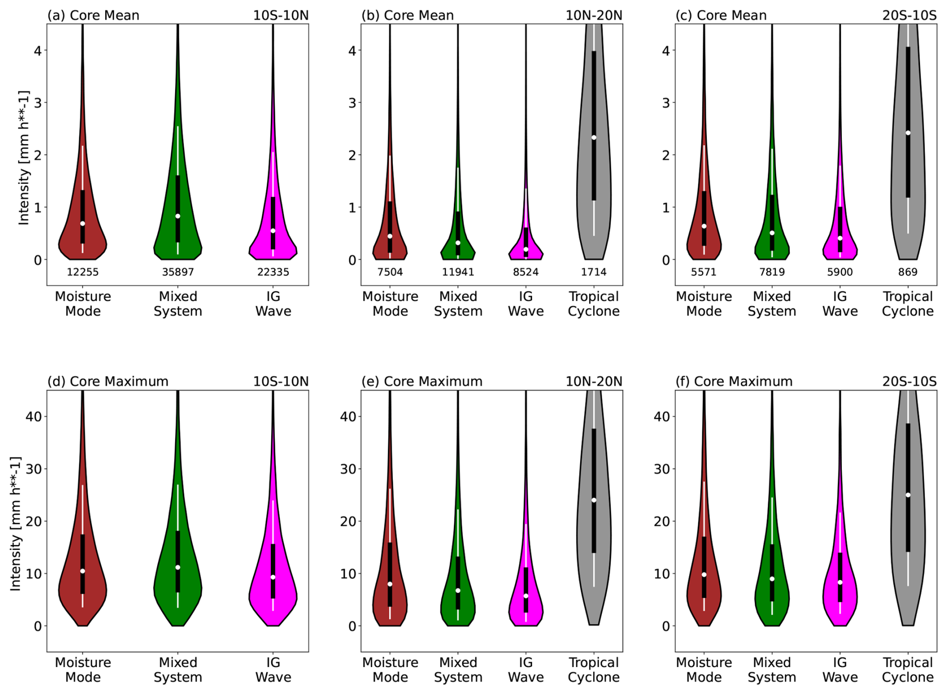
Figure 11 (a)–(c) Distributions of areal mean rainfall intensity within the cores of the tropical weather systems in the (a) equatorial, (b) northern hemisphere off-equatorial, and (c) southern hemisphere off-equatorial regions. (d)–(f) As in (a)–(c), but for areal maximum. The core of a system is defined as a 4° × 4° region around its detected centre at its “lag 0” time. The half-width of a violin at a rainfall intensity value represents its probability density (i.e., frequency of occurrence normalised by bin size). Numbers below each violin in (a)–(c) are their respective total counts. Note that we exclude TCs in the equatorial region due to limited number of samples, and that the y-axis ranges for (a)–(c) and (d)–(f) are different.

The fact that the systems we identify have characteristics of high rainfall intensity as described above means that their occurrences increase the chance of extreme rainfall intensity events (see Sect. 3 for the definition of an extreme event). This is shown in Fig. 12, which shows the likelihood change of an extreme event at a given location relative to a system's centre at the time of maximum OLR activity. In the equatorial region, extreme rainfall intensity events become 5.12 and 5.85 times more likely around the vicinity of moisture modes and mixed systems, respectively, whereas IG waves have a smaller but still significant impact of about a 300 % increase in extreme probability (Fig. 12a, d, g). This is in line with the previous results in Fig. 11, where mixed systems are associated with higher mean rainfall intensity than the other equatorial systems. Off the equator, however, moisture modes have a larger increase in extreme likelihood of up to 650 % around their centre (Fig. 12b–c), followed by mixed systems and IG waves. Note also that the region of influence (i.e., the spatial scale of the green shaded region) is larger for IG waves than for moisture modes because faster-moving systems travel further within the 3 h compositing period.

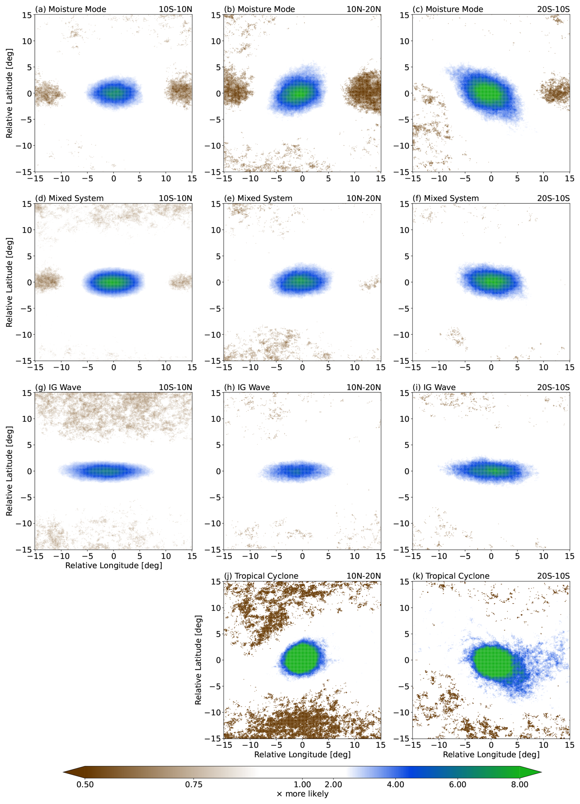
Figure 12 Probability ratio (see Eq. 3) of extreme rainfall intensity events associated with (a)–(c) moisture modes, (d)–(f) mixed systems, (g)–(i) IG waves, and (j)–(k) TCs in the (a, d, g) equatorial, (b, e, h, j) northern hemisphere off-equatorial, and (c, f, i, k) southern hemisphere off-equatorial regions. Only statistically significant values at 95 % level are shown, based on the two-tailed Student's t-test.

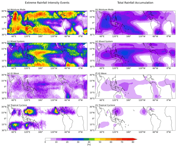
The extreme probability change analysis in Fig. 12, albeit indicating how strongly each type of system can modulate extreme rainfall occurrences, may not tell us the whole story of how impactful each system is to extreme rainfall in the tropics. For example, Fig. 12j, k show that TCs are associated with a much larger change in the likelihood of extreme events compared to the off-equatorial moisture modes (Fig. 12b, c). However, from Fig. 3, we know that the occurrence of TCs is much lower and less widespread than that of moisture modes in the off-equatorial regions. By also taking into account this frequency factor, in Fig. 13 we show that moisture modes are, in fact, associated with more extreme rainfall intensity events along the edges of the deep tropics. About 45 %–75 % of extreme rainfall intensity events in the 15–20° N/S region can be associated with moisture modes (we use the same attribution method as illustrated in Fig. 9). This number is about as large as that of extreme events associated with TCs in the TC-prone regions, such as the Philippines and off the west coast of Central America (Fig. 13g). In fact, in some regions that are commonly associated with TC occurrences like the Caribbean and the Bay of Bengal, moisture modes contribute a higher percentage of extreme rainfall events than TCs. This should give us some sense of how impactful the off-equatorial moisture mode is in terms of extreme 3-hourly rainfall events despite being only associated with only around 20 % of the region's total rainfall (Fig. 13b). For the equatorial region, the extreme events are more associated with mixed systems (Fig. 13c) and, to a much lesser extent, IG waves (Fig. 13e), as expected from the previous analyses. In the equatorial region, particularly along the Pacific ITCZ, high intensity rainfall events are disproportionately associated with mixed systems – these systems contribute almost half of the extreme rainfall (Fig. 13c), but only 30 % of the total rainfall (Fig. 13d).

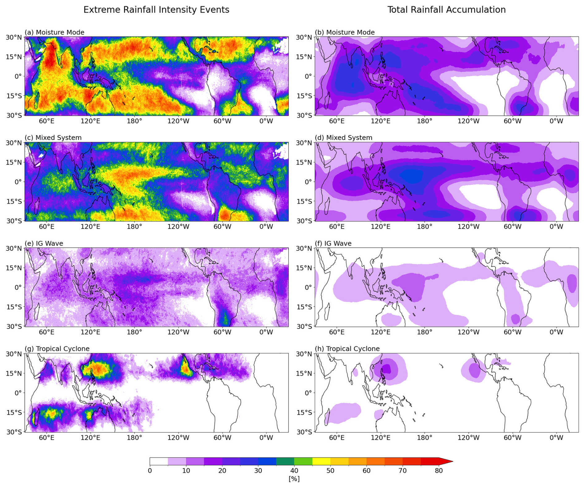
Figure 13 Percentages of (left) extreme rainfall intensity events and (right) total rainfall accumulation associated with (a)–(b) moisture modes, (c)–(d) mixed systems, (e)–(f) IG waves, and (g)–(h) TCs. Note that in some regions the sum exceeds 100 % as we do not exclude “compound” influences of more than one type of system.

6 Summary and Discussion

In this study, we divide the synoptic-to-planetary-scale convectively coupled systems in the tropics, other than TCs, into three categories based on their phase speed. The slow-moving systems are dominated by strong moisture perturbations and are called moisture modes. The fast-moving systems have weaker moisture anomalies but significant temperature perturbations, reminiscent of IG waves. The third category comprises systems with moderate propagating speed that have mixed characteristics of the other two, which we refer to as mixed systems. We employ this classification to define object-based weather systems in the tropics in a similar sense to those in the mid-latitudes. We find that moisture modes tend to occur along the edges of the deep tropics, confirming the hypothesis that a strong horizontal moisture gradient, as found along the climatological moist margin (e.g., Mapes et al., 2018; Robinson et al., 2024), is fundamental to their growth and propagation (Mayta and Adames Corraliza, 2024). On the other hand, mixed systems and IG waves are more commonly found closer to the equator, mostly along the ITCZ and especially over the Western Pacific warm pool. There are also some mixed system occurrences along the subtropical edges (i.e., 30° N/S), and these are likely to be the imprints of the moist QG system, which may be considered to be a mixed system with a small Rossby number and strong influences from the extratropics (Adames, 2022).

Analyses of the thermodynamic perturbation profiles show that the magnitude of moisture perturbations decreases from moisture modes to IG waves. However, the magnitude of temperature perturbations, here represented by the low-level DSE anomaly, does not seem to change with phase speed. Our results here support those of Adames et al. (2019) and Adames (2022) that the ratio of DSE to latent energy perturbation magnitudes (i.e., N_mode) increases from the slow-moving moisture mode to the fast-moving IG wave, as slower moving systems have a longer time scale allowing them to reach the WTG condition. We also find that this is mainly due to the changes in latent energy alone rather than in both moisture and DSE anomalies, consistent with Adames (2022). However, in contrast to Adames et al. (2019) and Adames (2022), we do not find that N_mode≫1 for IG waves, or even N_mode∼1 for mixed systems, indicating that some of the scaling values they used might be unrealistic. Rather, we find ratios closer to those found in Mapes et al. (2006), which are, expressed in g kg⁻¹:K units, about 1.6:1 for IG waves and 2:1 for mixed systems. In other words, the moisture perturbation does not become negligible in the faster-moving systems, but the relative importance of moisture and temperature does change with phase speed.

We also test the hypothesis that systems with similar thermodynamics (i.e., similar values of N_mode) can occur under different types of dynamical configuration or balance. Here we find that moisture modes in the equatorial region (10° S–10° N) have convergent-type dynamics, where the convectively active region is marked by the confluence of anomalous winds. Off the equator (10–20° N/S), the dynamics of moisture modes are more rotational, with the anomalous winds almost perfectly balancing the pressure perturbation field. A notable characteristic of the off-equatorial moisture mode is that its convectively active region is not collocated with its low-pressure centre as in TCs, but is shifted to over the poleward flow of the low-level vortex. This provides observational support for these slow-moving systems being energised by the moisture-vortex instability discussed in Adames and Ming (2018) and Mayta and Adames Corraliza (2024). Further evidence of this mechanism is found by focusing on the northern Indian ocean region in Boreal Summer. In this region, the moisture gradient is reversed, and this is associated with a shift of the ascent region of moisture modes to the western side of the disturbance, in line with the predictions of MVI theory. This signifies that the characteristics of moisture modes in particular, and perhaps the other tropical weather systems in general, are influenced by the underlying background state (see also e.g., Biswas et al., 2026). It is therefore worth exploring in future research how these characteristics might change under the changing background state due to warming. For example, some studies (e.g., Trenberth et al., 2005; Borger et al., 2022) indicate that the subtropical Western Pacific has a higher column water vapour trend than the equatorial Western Pacific. It remains an open question how this projected weakening of the meridional moisture gradient over the warm pool might change the frequency of occurrence as well as the characteristics of moisture modes over the region.

The distinction between equatorial and off-equatorial dynamics is also seen in mixed systems, but becomes less discernible in IG waves. For both equatorial and off-equatorial systems, we find that the proximity to nonlinear balance (e.g., Bolin, 1955; Charney, 1955) decreases with phase speeds; faster-moving systems tend to be more unbalanced than slower-moving systems, consistent with the theory of Adames (2022). We therefore conclude that, as in the thermodynamics, there is also a dynamical spectrum from the balanced moisture modes to the unbalanced IG waves.

Connecting back to our main motivation laid out in the Introduction, we argue that our study here is an attempt to define a set of synoptic-scale weather systems in the tropics analogous to those in the extratropics. As in the extratropics, continuous atmospheric waves are the “background” dynamics of the weather. For example, a typical Rossby wave train in the midlatitudes can give rise to several pairs of high- and low-pressure systems. These highs and lows are the extratropical “weather systems”, not the Rossby wave itself. These synoptic-scale systems are the bridge between the planetary-scale background dynamics and the smaller-scale tangible weather occurrences, such as thunderstorms and wind gusts. Applying this idea to the tropics, we posit that equatorial waves, including the MJO, are the dynamics occurring in the “background”, and they can spawn synoptic-scale weather systems investigated in this study. For instance, ER waves are characterised by sets of gyres, and, among these, the cyclonic gyres may be identified as moisture mode “objects”, or may amplify and become TCs (e.g., Frank and Roundy, 2006; Feng et al., 2023). Furthermore, as different types of waves commonly co-occur, our methods here implicitly take into account the interactions among different waves in the same phase speed category, which are argued to have similar thermodynamic characteristics, when we do the spectral filtering. In this way, a detected synoptic “object” may be a manifestation of those interactions in the background, rather than representing only a single type of wave.

The characteristics of the weather systems we define, including their dominant dynamical balances, phase relations between vertical and horizontal motion, and thermodynamic structure are broadly consistent with the prototype weather systems described in Adames (2022) based on a theoretical scaling of the governing equations. This suggests that the moisture mode-to-gravity wave spectrum provides a useful framework for separating tropical systems by their dynamics.

Another aspect of the three types of weather system that we study here is their impacts on tropical rainfall, especially on rainfall events that are considered extreme. The synoptic weather systems defined here (including TCs) are associated with almost 60 % of total rainfall received in the deep tropics and mainly with events with high rainfall accumulation. Moisture modes are particularly important for precipitation in the off-equatorial regions, where they are associated with 45 %–75 % of extreme 3-hourly rainfall events, almost as much as TCs in TC-prone regions. On the other hand, mixed systems and, to a lesser extent, IG waves are more important for precipitation in the equatorial regions, especially along the Pacific ITCZ. These results provide a new insight on the relationship between atmospheric phenomena and precipitation in the tropics. Past studies usually only attributed most of the tropical mean and extreme precipitation to MCSs and TCs (see e.g., Dowdy and Catto, 2017; Utsumi et al., 2017; Zhao, 2022; Prein et al., 2023; Tsai et al., 2025). Here, we aim to define weather systems on synoptic scales similar to the scales of TCs, and we therefore do not consider MCSs directly. Rather, we present the attribution of rainfall to the three systems comprising the moisture mode-to-gravity wave spectrum.

Finally, we note some caveats of the weather system identification we present. By decomposing based on phase speed, we may “split” a robust signal of a coherent object just because it moves with speed close to the phase speed threshold we prescribe in our methods. Furthermore, we decompose objects by zonal phase speed, and objects with substantial meridional phase speed may be misrepresented as having lower phase speed. Additionally, our fundamental assumption that phase speed is a proxy for thermodynamics also has some limitations. As mentioned in Sect. 2, Eq. (2) comes from a reasonable assumption that ${\text{Fr}}_{\mathit{\tau }}^{\mathrm{2}}>{\text{Bu}}^{-\mathrm{1}}$ for typical synoptic-scale systems near the equator. This approximation becomes less valid for systems occurring farther from the equator, as illustrated in the following example. A moisture mode system with L_x, L_y∼1000 km occurring at 10° latitude will have a Burger number of about Bu≈150, and therefore ${\text{Fr}}_{\mathit{\tau }}^{\mathrm{2}}$ will always be greater than Bu⁻¹ for this slow-moving category (c_p≲9 m s⁻¹). However, if the same system occurs at 25° latitude, its Burger number will be Bu≈26, and ${\text{Fr}}_{\mathit{\tau }}^{\mathrm{2}}$ will no longer be greater than Bu⁻¹. We attempt to avoid these systems for which the approximation in Eq. (2) is invalid by only including systems whose centroids are not beyond 20° latitude in the off-equatorial moisture mode composites, but even then systems with L_y≳1200 km will have ${\text{Fr}}_{\mathit{\tau }}^{\mathrm{2}}\lesssim {\text{Bu}}^{-\mathrm{1}}$ and $N_{\text{mode}}\gtrsim {\mathrm{10}}^{-\mathrm{0.5}}$. Therefore, our results on off-equatorial moisture modes should be treated and interpreted more carefully, as they are likely to be “contaminated” by systems technically belonging to the mixed system category.

While the theory hypothesises that systems with similar N_mode have similar thermodynamics, observational studies have shown that eastward- and westward-propagating disturbances with similar phase speed can have different vertical profiles and phase tilts (e.g., Inoue et al., 2020). Since our compositing technique combines both eastward- and westward-propagating disturbances, it can hide such phase tilts or other asymmetries associated with the direction of phase propagation. However, separating the eastward- and westward-propagating signals (see Supplement) does not change the general conclusions described above.

Another caveat of this study is that we use OLR to represent convective signals. Even though OLR has long been used, and is still widely used, to study large-scale convectively coupled signals in the tropics, it is not objectively the best variable to use, as some large stratiform-cloud covered areas may also be captured as strong OLR activity. The 3-hourly time resolution of the ISCCP dataset we use is also a limitation, and may not be sufficient to capture the fastest-moving IG wave signals. In addition to these, we also recognise that the removal of diurnal cycle excludes the most important rainfall-related processes over coastal areas and islands. Moreover, this could also underestimate the activity of IG wave, as some previous studies (e.g., Takayabu et al., 1996; Chen and Houze Jr, 1997; Liebmann et al., 1997) suggest that this fast-moving system is tightly connected to diurnal convective activity. Nevertheless, we believe that this study provides an important step towards a coherent description of synoptic weather in the tropics from a more object-based weather system perspective. This study is also the first one to apply the theoretical framework of a moisture mode-to-gravity wave spectrum towards this goal. Future research could use this framework to assist extreme weather forecasting, help understand tropical rainfall changes in a warmer climate, and contribute to our understanding of the complex relation between large-scale dynamics and convection in the tropics.

Appendix A: Relating N_mode to the Speed of a Disturbance

Here we show that the parameter N_mode may be written in terms of the phase speed of a disturbance. To do so, we perform a scale analysis of temperature and humidity anomalies in the atmosphere following Adames et al. (2019). Assuming a dominant balance in the momentum equation between the geopotential gradient and the velocity tendency we may write,

$$\begin{array}{}\text{(A1)}& {\displaystyle \frac{{\mathrm{\Phi }}^{\prime }}{L}}\sim {\displaystyle \frac{U^{\prime }}{\mathit{\tau }}},\end{array}$$

where Φ^′ and U^′ are the scales for geopotential anomalies and horizontal velocity anomalies, and L and τ are characteristic length and time scales. We follow Adames et al. (2019) and assume that the time and length scales are related by the phase speed of the disturbance $c_{\mathrm{p}}=L/\mathit{\tau }$, so that

$$\begin{array}{}\text{(A2)}& {\mathrm{\Phi }}^{\prime }\sim U^{\prime }{c}_{\mathrm{p}}.\end{array}$$

The geopotential is related to temperature via the hydrostatic equation

$$\begin{array}{}\text{(A3)}& {\displaystyle \frac{\partial {\mathrm{\Phi }}^{\prime }}{\partial p}}=-{\displaystyle \frac{R_{\mathrm{d}}{T}^{\prime }}{p}}.\end{array}$$

For a disturbance spanning the depth of the troposphere, this implies

$$\begin{array}{}\text{(A4)}& T^{\prime }\sim {\displaystyle \frac{{\mathrm{\Phi }}^{\prime }}{R_{\mathrm{d}}}}\end{array}$$

Following Adames et al. (2019), we may write this in terms of c, the phase speed of the first-baroclinic gravity wave,

$$\begin{array}{}\text{(A5)}& T^{\prime }\sim {\displaystyle \frac{\mathrm{\Delta }s}{C_{\mathrm{p}}{c}^{\mathrm{2}}}}{\mathrm{\Phi }}^{\prime },\end{array}$$

where Δs is the vertical difference in dry static energy over the troposphere.

Finally, we derive a scaling for specific humidity anomalies q^′. To do so, we assume the leading order balance in the moisture equation is between vertical moisture advection and precipitation. We further assume that precipitation acts to remove humidity anomalies over a timescale τ_c. We then have,

$$\begin{array}{}\text{(A6)}& W{\displaystyle \frac{\mathrm{\Delta }q}{H}}\sim {\displaystyle \frac{q^{\prime }}{{\mathit{\tau }}_{\mathrm{c}}}}\end{array}$$

where W is the vertical velocity scale, Δq is the vertical difference in specific humidity over the troposphere and H is the depth of the troposphere. Mass continuity implies that the the vertical velocity is related to the horizontal velocity as $W/H\sim U/L$, giving

$$\begin{array}{}\text{(A7)}& U{\displaystyle \frac{\mathrm{\Delta }q}{L}}\sim {\displaystyle \frac{q^{\prime }}{{\mathit{\tau }}_{\mathrm{c}}}}\end{array}$$

Combining Eqs. (A2), (A5), and (A7) gives,

$$\begin{array}{}\text{(A8)}& N_{\text{mode}}={\displaystyle \frac{C_{\mathrm{p}}{T}^{\prime }}{L_v{q}^{\prime }}}\sim {\displaystyle \frac{c_{\mathrm{p}}^{\mathrm{2}}}{c^{\mathrm{2}}}}{\displaystyle \frac{\mathrm{1}}{N_{\mathrm{c}}\widehat{\mathit{\alpha }}}},\end{array}$$

where we have identified $\mathrm{\Delta }s/L\mathrm{\Delta }q=\widehat{\mathit{\alpha }}$ and defined $N_{\mathrm{c}}={\mathit{\tau }}_{\mathrm{c}}/\mathit{\tau }$. This equation shows that N_mode scales with the square of the phase velocity of a disturbance.

Note that the above derivation is limited to the tropical regime, in which one may neglect the possible influence of the Coriolis force on the scaling of geopotential anomalies, and it assumes N_c does not depend on the phase speed of the disturbance. A more comprehensive scaling analysis that does not make either of these assumptions may be found in Adames (2022), in which a similar scaling for N_mode is found and is employed in Eq. (2), provided the Burger number is sufficiently large as detailed in the manuscript.

Appendix B: Parameters of tobac's Identification and Tracking Functions

Below are the detailed parameters we use to run the algorithm. For more details, see tobac's documentation (https://tobac.readthedocs.io, last access: 8 April 2026).

• parameters_features is used in the object identification step. tobac allows for multiple thresholds to better capture multiple objects that are connected through a contiguous region of less restrictive threshold values. As we aim to detect strong negative OLR anomaly objects, we set the target to be minimum. We choose weighted_diff as the position_threshold so that every object's location is represented by its centroid. To avoid detecting noise, we apply a moderate two-dimensional Gaussian filter (sigma_threshold = 1.0) prior to object identification, and reject any detected object with less than 4 connected grid points (n_min_threshold = 4). Lastly, we set the second horizontal dimension of the field (hdim_2, which is longitude) to be periodic.

    parameters_features["threshold"]
    = [-2.0, -2.5, -3.0, -3.5, -4.0] * olr_std_dev
    parameters_features["target"] = "minimum"
    parameters_features["position_threshold"]
    = "weighted_diff"
    parameters_features["sigma_threshold"] = 1.0
    parameters_features["n_min_threshold"] = 4
    parameters_features["PBC_flag"] = "hdim_2"

• parameters_linking is used in linking two detected objects in subsequent time steps in the tracking step. v_max is the maximum propagating speed of each system type as described in Sect. 3, that is, 9, 27, 50, and 10 m s⁻¹ for moisture modes, mixed systems, IG waves, and TCs, respectively. We set stubs = 3 to disregard any track with a lifetime of less than 3 subsequent time steps (i.e., 9 h). As in parameters_features, we set hdim_2 (i.e., longitude) to be periodic from min_h2 = 0 to max_h2 = len(longitude) - 1.

    parameters_linking["v_max"] = v_max
    parameters_linking["stubs"] = 3
    parameters_linking["PBC_flag"] = "hdim_2"
    parameters_linking["min_h2"] = 0
    parameters_linking["max_h2"] = len(longitude) - 1

• parameters_segmentation is used in determining the detected objects' boundaries. For this routine, tobac only accepts a single threshold, so we choose the least restrictive value.

    parameters_segmentation["threshold"]
    = -2.0 * olr_std_dev
    parameters_segmentation["target"] = "minimum"
    parameters_segmentation["PBC_flag"] = "hdim_2"