Deficient ocean–atmosphere feedbacks constrain seasonal NAO prediction

As the North Atlantic Oscillation (NAO) accounts for a dominant share of wintertime weather variability across the North Atlantic, it is a coveted target for seasonal prediction. Yet dynamical forecast systems exhibit limited skill. Here I build on previous results linking November sea-surface temperature (SST) anomalies to the subsequent winter NAO via ocean–atmosphere feedback mechanisms involving baroclinicity and surface heat fluxes. I hypothesise that limited model skill is partly attributable to a deficient representation of these mechanisms. While remote influences such as tropical or stratospheric forcing can affect both SSTs and the NAO, thereby contributing to apparent but non-causal relationships, I find that the seasonal prediction system SEAS5's internal lagged SST–NAO relationship nonetheless correlates with its NAO forecast skill. Since this skill reflects the combined effects of all sources of predictability – including tropical and stratospheric forcing – this correlation is an important finding. Using mediation analysis to contrast the behaviour of SEAS5 with that of the ERA5 reanalysis, I find that SEAS5 produces weaker mediated effects via both fluxes and baroclinicity than those found in ERA5. Critically, the strength of these mediated effects in the model correlates with its NAO forecast skill. This suggests that models reproducing realistic mediation pathways for ocean–atmosphere interactions are likely to achieve higher NAO skill than models that do not.

1 Introduction

It is no wonder that the North Atlantic Oscillation (NAO) has received considerable attention in studies of climate dynamics, given that it accounts for roughly half of the interannual wintertime tropospheric pressure variance over the North Atlantic (Ambaum et al., 2001). Hence, it serves as a good proxy for fluctuations in the strength and latitudinal position of the jet stream (Woollings and Blackburn, 2012) and storm tracks (Rivière and Orlanski, 2007), and by extension for variations in weather and associated impacts over and around the North Atlantic basin (e.g. Athanasiadis et al., 2017; Degenhardt et al., 2023).

Owing to its wide-ranging influence, the NAO is routinely used as a benchmark for mid-latitude seasonal prediction skill. Statistical (empirical) methods have a long history and have achieved potentially useful levels of skill using predictors such as autumn Arctic sea ice, Eurasian snow cover, tropical and regional sea-surface temperatures (SSTs), and stratospheric variables (e.g. Hall et al., 2017; Wang et al., 2017). While empirical models offer interpretability and have at times appeared to outperform dynamical systems, their reliance on historical relationships makes them vulnerable to non-stationarity and shifts in climate regimes (Hertig et al., 2015; Kolstad and Screen, 2019). Demonstrated skill in one period therefore provides no guarantee of consistent predictability in others (Weisheimer et al., 2017; Baker et al., 2024). More recently, empirical models have been enriched with machine-learning and hybrid techniques, yielding higher forecast skill, including for the NAO (e.g. Mu et al., 2023; Sun et al., 2024).

In sum, empirical models are susceptible to including non-causal predictors, either because background-state changes render previous relationships invalid or due to spurious correlations. In principle, dynamical coupled prediction systems are not constrained by these limitations, as they aim to reproduce the behaviour of the climate system from first principles. Such systems should ideally be able to integrate any initial condition to a realistic future state. In practice, however, as Suckling and Smith (2013) pointed out, even physics-based models are not independent of the data used in their design. Their apparent ability, evaluated primarily through retroactive forecasts, or reforecasts (also known as hindcasts), to reproduce historical variability may therefore overstate true predictive skill. Moreover, in a changing climate, even out-of-sample performance offers no guarantee of future success, given the nonlinear nature of the system's response to external forcing (Stott et al., 2013). This highlights the need to assess not only the overall skill of prediction systems, but also the physical consistency of the processes and feedbacks they represent.

About a decade ago there was a surge of enthusiasm over the high surface-defined NAO skill reported in some dynamical systems (Scaife et al., 2014). However, there is a wide range of performance between systems and system upgrades have not significantly improved overall skill (Baker et al., 2024). Several studies have convincingly demonstrated that the performance of dynamical prediction systems depends on how well they represent crucial physical processes. For instance, Patrizio et al. (2025) showed that skill in decadal NAO forecasts depends on how models represent feedbacks between subpolar SST anomalies and the NAO. Haarsma et al. (2019) found that increasing the oceanic resolution of a coupled system strengthened air–sea interactions and enhanced seasonal predictability in the North Atlantic storm track entrance region east of Newfoundland. Similarly, Hardiman et al. (2022) showed that most forecast systems consistently underestimate positive feedback mechanisms between transient eddies and the large-scale flow, leading to weaker eddy forcing of the mean circulation. A related problem concerns the representation of mesoscale oceanic eddies and associated SST gradients in “eddy-rich regions, including the Gulf Stream” (Zhang et al., 2021). Limited horizontal resolution tends to smooth these gradients and weaken the coupling between SST, surface heat fluxes, and low-level atmospheric baroclinicity (Hewitt et al., 2017; Bellucci et al., 2021; Athanasiadis et al., 2022).

Together, these findings highlight that two-way ocean–atmosphere coupling is fundamental to NAO variability across timescales, yet it remains misrepresented in current prediction systems. Indeed, for the same family of forecast systems considered here, Roberts et al. (2021) demonstrated that biases in the location and structure of the Gulf Stream substantially degrade subseasonal forecast skill, and that correcting these SST errors online improves the mean state and circulation anomalies across the North Atlantic and downstream into Europe.

A large body of work has convincingly shown that, in the North Atlantic, the atmospheric impact on the ocean surface generally dominates the feedback loop. For instance, Patterson et al. (2024) recently demonstrated that the atmosphere primarily drives surface heat flux variability in the Labrador Sea. However, the same study identified a strong oceanic imprint on the atmosphere further south in the Gulf Stream region. Similarly, Joyce et al. (2019) demonstrated that meridional shifts of the Gulf Stream front and its associated SST gradients tend to lead changes in storm tracks and Greenland blocking by one to three months, suggesting an evolving pathway from autumn ocean conditions to wintertime atmospheric variability. Both observational studies (Czaja and Frankignoul, 2002; Wang et al., 2004; Hall et al., 2017) and modelling experiments (Rodwell et al., 1999; Watanabe and Kimoto, 2000; Baker et al., 2019; Sun et al., 2024) have shown that characteristic SST patterns can precondition the atmosphere on subseasonal to seasonal timescales. In particular, the North Atlantic SST tripole (or the similar “horseshoe” pattern) has been linked to a feedback loop involving the NAO itself (Peng et al., 2002; Pan, 2005; Mosedale et al., 2006; Cassou et al., 2007; Gastineau and Frankignoul, 2015).

A useful distinction emerging from this literature is that observational studies identify these SST–atmosphere linkages directly in the climate record, whereas model-based studies generally recover similar patterns only when the predictable component of variability is isolated. This reflects signal-to-noise issues (Scaife and Smith, 2018; Weisheimer et al., 2024): models can reproduce the relevant mechanisms, but the forced signal is often weaker than in observations, making the pathways more difficult to detect.

Kolstad and O'Reilly (2024) used reanalysis data to demonstrate that the correlation between November SSTs and the subsequent NAO increases gradually through the winter season, peaking in January and February. They showed that surface heat fluxes in the western part of the Subpolar Gyre region and baroclinicity in the storm track entrance region in the western North Atlantic act as key mediators in this feedback. The latter result is consistent with the well-established role of diabatic heating and eddy feedbacks in maintaining storm track baroclinicity (Hardiman et al., 2022).

The statistical framework used by Kolstad and O'Reilly (2024) is known as mediation analysis (e.g. MacKinnon et al., 2000; Nguyen et al., 2021). It is particularly well-suited to climate science applications where feedback loops and mediated pathways are common but difficult to isolate using traditional correlation-based methods. Recent examples of its use, in additon to some of my own work, include the studies by Maybee et al. (2023) and Risser et al. (2025). The framework belongs to the broader family of causal inference methods (Pearl et al., 2016), so named because they are designed to identify and quantify causal relationships. Several such approaches have been successfully used in climate science, ranging from easily interpretable approaches like Granger causality (e.g. Granger, 1969; Mosedale et al., 2006; McGraw and Barnes, 2018) to more complex methods (e.g. Ebert-Uphoff and Deng, 2012; Hannart et al., 2016; Runge et al., 2019; Docquier et al., 2024).

A key advantage of causal inference approaches is that they allow pathways to be investigated without manipulating model boundary conditions for sensitivity experiments. Perturbation-based methods, though widely used, can produce unintended consequences. For example, perturbing greenhouse gas concentrations triggers numerous feedbacks on diverse timescales, complicating attribution of the climate system's response and adjustments (Knutti and Rugenstein, 2015). Even more localised interventions can have undesirable side effects: Lewis et al. (2024) showed that modifying albedo or applying surface heating to force sea-ice loss can generate spurious warming and exaggerate the atmospheric circulation response. Similarly, O'Reilly et al. (2023) demonstrated that active SST-restoring in the tropical North Atlantic can systematically drive upward surface heat fluxes that are unrepresentative of observations, leading to an exaggerated precipitation and remote circulation response. As Palmer and Weisheimer (2011) noted, multiple model errors can compensate for one another, making it difficult to diagnose the underlying causes of biases. These considerations further motivate the use of mediation analysis, which relies solely on observed covariances and avoids imposing artificial perturbations.

This study extends Kolstad and O'Reilly (2024) in three ways. First, it examines whether the strength of the November-to-winter SST-NAO linkage in a state-of-the-art seasonal forecast system is related to its skill in predicting the NAO, thereby motivating the subsequent mediation analysis. Second, it quantifies and clarifies causal directionality in the relationships between November SSTs and surface heat fluxes, baroclinicity, and the winter NAO. Third, it applies the mediation framework to the forecast system to assess whether biases in these relationships can help explain its limited NAO prediction skill.

It is important to emphasise that the mediation pathways examined here do not account for the full influence of November SSTs on the winter NAO, which can be viewed as the combined effect of all possible pathways operating throughout the climate system, both locally and remotely. The present analysis focuses on only a small subset of this much broader interaction network. It zooms in on surface heat fluxes and baroclinicity because there are good physical reasons to expect these mechanisms to participate in SST-induced adjustments of the North Atlantic circulation. In other words, the analysis should be interpreted as isolating two components of the total SST influence: it has the potential to reveal where these specific pathways reinforce or oppose the SST–NAO relationship, without implying that they represent the full climate system’s response. It is furthermore acknowledged that remote effects such as the El Niño–Southern Oscillation (ENSO) may influence both the SSTs and the NAO and thereby contribute to apparent but non-causal associations within the SST–mediator–NAO relationship.

The following section gives an overview of mediation and partial-correlation analysis, before the data and methods are described in Sect. 3. Section 4 presents the results, and Sect. 5 discusses their implications for understanding and improving NAO predictability.

2 Mediation analysis

Adopting the naming convention of MacKinnon et al. (2000), a causal pathway linking a predictor variable X to an outcome variable Y is written as:

$$X\to Y.$$

In the analysis to follow, X is an index representing SST anomalies in November and Y is the winter NAO index. Due to the temporal offset, the correlation between these two variables must be mediated by other processes, referred to as mediators and denoted Z. Here Z is a gridded spatial field representing surface heat fluxes and a metric for baroclinicity. These mediators are investigated separately through the pathway

$$X\to Z\to Y.$$

It is customary to quantify the mediating role of Z and categorizing it as either: a perfect or partial mediator if it fully or partially accounts for X→Y (Baron and Kenny, 1986); or a suppressor if the correlation between X and Y is strengthened when Z is accounted for (Conger, 1974).

As mentioned in the Introduction, a pixel value of any one variable cannot uniquely mediate the lagged effect of SSTs on the NAO. In reality, a practically infinite web of interacting processes combine to realise that relationship. Nevertheless, the approach used here is useful for providing a spatial fingerprint of where a single variable exerts the strongest mediating influence. Equally important, the method can be used to identify where a forecast model incorrectly mediates or even suppresses the SST–NAO correlation.

2.1 Regression equations

To test for mediation or suppression, three regression equations are defined (ignoring intercepts and residuals for simplicity). Prior to estimating the coefficients, X, Y, and Z were standardised. The first equation describes the total effect τ of the predictor X on the predictand Y:

$$\begin{array}{}\text{(1)}& Y=\mathit{\tau }X.\end{array}$$

Here, τ represents the correlation between the standardised November SST index and the standardised winter NAO index. The second regression describes $X\to Z\to Y$ by accounting for the standardised mediator variables. The effect of X on Y changes to τ^′, known as the direct effect (not through the mediator), and the effect of Z on Y when accounting for X is denoted as β:

$$\begin{array}{}\text{(2)}& Y={\mathit{\tau }}^{\prime }X+\mathit{\beta }Z.\end{array}$$

The total effect of X on the mediator Z is labelled here as α in the second equation:

$$\begin{array}{}\text{(3)}& Z=\mathit{\alpha }X.\end{array}$$

An important thing to note is that α encapsulates not just the direct forcing X→Z, but also all the indirect forcing through intermediate variables, crucially including via the pathway $X\to Y\to Z$.

A central concept is the product αβ, known as the indirect or mediated effect (of X on Y through Z). The total effect is the sum of the direct and mediated effects: $\mathit{\tau }={\mathit{\tau }}^{\prime }+\mathit{\alpha }\mathit{\beta }$. This also follows from Eqs. (1)–(3). Scaling the mediated effect by the total effect yields:

$$\begin{array}{}\text{(4)}& {\displaystyle \frac{\mathit{\alpha }\mathit{\beta }}{\mathit{\tau }}}=\mathrm{1}-{\displaystyle \frac{{\mathit{\tau }}^{\prime }}{\mathit{\tau }}}.\end{array}$$

According to the standard criteria for mediation laid out by Baron and Kenny (1986), τ, α, and β must all be significantly different from zero. If ${\mathit{\tau }}^{\prime }=\mathrm{0}$ (or is not significantly different from zero), it follows from Eq. (4) that the total and mediated effects are identical. In this case, the pathway X→Y is fully accounted for by Z, indicating that $X\to Z\to Y$ represents a valid causal pathway – though not necessarily the only one.

2.2 Identifying the SST-forced component

Mediation often represents forward-directed pathways where X changes Z, and Z subsequently affects Y. In climate dynamics, however, feedback mechanisms are common, and ambiguities may arise because Y and Z are evaluated contemporaneously. This implies that both the hypothesised $X\to Z\to Y$ and the alternative $X\to Y\to Z$ pathways may be active. It is nevertheless possible to assess the degree to which Z responds directly to X rather than indirectly through Y by regressing out the concurrent variability of Y:

$$\begin{array}{}\text{(5)}& Z={\mathit{\alpha }}^{\prime }X+\mathit{\gamma }Y.\end{array}$$

Here, α^′ represents the NAO-independent SST-to-mediator influence, to be compared with α from Eq. (3), which includes all routes from X to Z (including those via Y). The product α^′β is then interpreted as the SST-forced component of the mediated effect; that is, the influence that would arise if the mediator responded only to direct SST forcing, while the NAO retained its full sensitivity to the mediator through β. This is a complementary diagnostic to the full mediated effect αβ, not a replacement; it helps distinguish SST-forced mediation from mediation that is predominantly atmospheric in origin.

To quantify the SST forcing onto the mediator, the sign consistency between α^′ and α is assessed. In regions where the SST forcing aligns with the full forcing (which includes NAO feedbacks on Z), the ratio ${\mathit{\alpha }}^{\prime }/\mathit{\alpha }$ should be positive. Values near zero indicate that the SST forcing is weak. Because the mediators (Z) are inherently noisy, Ordinary Least Squares (OLS) estimates of α and α^′ are both subject to attenuation bias (Greene, 2003), which biases coefficients towards zero and increases the chance of sign flips across different sample sets.

Accordingly, I use a conservative hypothesis test: the null hypothesis is that the SST-forced component (α^′) is zero or has the opposite sign to the total forcing onto the mediator (α). Rejecting this null hypothesis indicates that the SST forcing is sufficiently robust to maintain a consistent physical direction despite attenuation. I emphasise that it does not imply that the SST forcing dominates over NAO → mediator feedbacks.

Accounting for the NAO's autocorrelation is another prudent step to prevent potential confounding of the results. Kolstad and O'Reilly (2024) showed that in ERA5, this autocorrelation was only significant from November to December and not from November to DJF; this was confirmed to be valid for the shorter period examined here for both ERA5 and SEAS5. Labelling the NAO index in November as Y₀, a new regression equation could be defined as:

$$Z={\mathit{\alpha }}^{\prime \prime }X+{\mathit{\gamma }}_{\mathrm{0}}{Y}_{\mathrm{0}}+{\mathit{\gamma }}^{\prime }Y.$$

However, as the coefficient γ₀ was found to be negligible for both mediators, which was expected in light of the missing NAO autocorrelation, Eq. (5) is used in the analysis.

2.3 Suppression

An interesting special case occurs when ${\mathit{\tau }}^{\prime }/\mathit{\tau }>\mathrm{1}$, which means that the mediated effect αβ has the opposite sign to the total effect τ (Eq. 4). In these cases, Z is referred to as a suppressor because the regression coefficient linking X and Y is inflated when Z is accounted for (Muniz and MacKinnon, 2025). In the context of this study, this could mean that X (November SST anomalies) drives changes in Z (e.g. flux anomalies), but the response of Y (the NAO) to those fluxes is of opposite sign to the direct X→Y pathway. This can occur because Y itself feeds back onto Z, helping to make β negative. In other words, Z acts as a negative feedback, transmitting a damping influence on Y that partly cancels (suppresses) the predictive signal from X. In the raw correlation, this feedback reduces the apparent strength of X as a predictor of Y, but once Z is controlled for, the hidden strength of the X→Y link is revealed. Put differently, had it not been for the negative feedback through Z, X would have exerted stronger predictive power on Y.

2.4 Scope

The mediation framework is applied to X, Z and Y as defined over the North Atlantic sector. Controls for remote precursors such as ENSO or stratospheric anomalies are not included. Consequently, any shared influence of such processes on both pre-winter SST and the winter NAO can appear implicitly in the estimated relationships; the results should therefore be interpreted as structural diagnostics rather than formal causal attribution across the full suite of teleconnections.

2.5 Sample coefficient notation

Throughout the paper, sample coefficients in Eqs. (1)–(5) (i.e. coefficients estimated through OLS fitting) are denoted by carets; for instance, $\widehat{\mathit{\tau }}$ is the estimated τ value.

3 Data and methods

3.1 Data

Reanalysis and seasonal forecast data are used. The reanalysis reference is ERA5 (Hersbach et al., 2020), produced by the European Centre for Medium-range Weather Prediction (ECMWF), and the forecast system is SEAS5, the ECMWF's seasonal prediction system (Johnson et al., 2019). The reason only one model is investigated here is that its reforecast period extends back to 1981, while reforecasts are only available from 1993 and onwards for comparable systems – this shorter period would render the mediation analysis less robust. The analysis covers the winters from 1981/82 to 2023/24 (hereafter referred to as 1981–2023).

The atmospheric component of SEAS5 is the Integrated Forecast System (IFS) atmosphere model. The grid spacing for the ocean model in SEAS5 is 0.25 degrees, which has been shown to yield a decent representation of air–sea interaction along the Gulf Stream front compared to lower-resolution models (Jin and Yu, 2013; Athanasiadis et al., 2022; Patrizio et al., 2023). It seems the resolution will not change in the new SEAS6 system due to be released soon, but the new ocean model nevertheless appears to yield multiple improvements, including large reductions in SST errors along the Gulf Stream (Keeley et al., 2024, their Fig. 2a).

A well-documented feature of SEAS5 relevant for this study is a warm SST bias in the western North Atlantic up to the mid-1990s (Stockdale et al., 2018; Tietsche et al., 2020). Inherited from issues with the ocean reanalysis, this bias allowed SST errors to grow rapidly and produced a local warm anomaly that affected near-surface temperature and surface heat fluxes. To verify that it did not affect the conclusions of this paper, the core analysis was repeated using only the period 2001–2023; the results were practically unchanged.

SEAS5 reforecasts were used from 1981 to 2016 with 25 ensemble members, and real-time forecasts from 2017 to 2023 with only the first 25 of 51 members used to ensure consistency with the reforecasts. The analysis was based on individual ensemble members (i.e. not ensemble means) unless otherwise specified.

SEAS5 forecasts are issued once per month. In this study, the November forecasts and reforecasts are used, corresponding by convention to lead times of 1–4 months for November through February. A potential drawback of using the November initialisations is that the SST fields are similar across ensemble members due to oceanic inertia. However, repeating the complete analysis with October initialisations (for which the November SST fields are more diverse) produced qualitatively similar results. I chose to base the analysis on the November runs, as this allows evaluation of the model's skill for the set of forecasts used operationally for predicting winter conditions.

The variables considered are SST, mean sea level pressure (SLP), and the sum of sensible and latent heat flux, hereafter referred to as surface heat flux, or SHF (positive upwards). Baroclinicity is quantified by the Eady growth rate maximum (e.g. Hoskins and Valdes, 1990), defined for the 700–850 hPa layer as

$${\mathit{\sigma }}_{\mathrm{E}}=cf\left|{\displaystyle \frac{\partial \mathit{v}}{\partial z}}\right|/N,$$

where the unit is day⁻¹, c=86 400×0.3098, f is the Coriolis parameter, v is the wind vector, z is the geopotential height, and N is the Brunt-Väisälä frequency, given by

$$N=\sqrt{{\displaystyle \frac{g}{\mathit{\theta }}}{\displaystyle \frac{\partial \mathit{\theta }}{\partial z}}},$$

with θ the potential temperature and g the gravitational acceleration.

Anomalies were calculated by subtracting the overall mean and dividing by the overall standard deviation, spanning all years and ensemble members.

3.2 Climate indices

Two scalar indices are central to the analysis: the DJF NAO index, and an SST-based index representing the November SST anomaly pattern in the extratropical North Atlantic most strongly correlated with the following winter's NAO index.

To construct the NAO index, the first Empirical Orthogonal Function (EOF) of interannual DJF mean ERA5 SLP anomalies was computed over the domain 20–80° N, 90° W–40° E, using the eofs Python package (Dawson, 2016) and applying $\sqrt{\cos \mathit{\varphi }}$ latitude weighting. For both ERA5 and SEAS5, the corresponding NAO index time series were obtained by projecting their respective gridded SLP anomalies onto the ERA5-based spatial EOF pattern. It was a deliberate choice to use the ERA5 loading pattern for both datasets, as the purpose of this study is to assess how SEAS5 represents the real-world NAO pattern.

The SST index was calculated in a similar way. November SST anomalies from ERA5 were first regressed onto the interannual ERA5 NAO index to obtain a spatial regression pattern. SST anomalies were then projected onto this pattern within a reference domain extending from the 20 to 70° N and from 100° W to 20° E (Czaja and Frankignoul, 2002; Kolstad and O'Reilly, 2024), after which the resulting series was standardised to form the SST index. As with the NAO index, the SST index for SEAS5 was computed by projection onto the ERA5-based pattern, not a model-specific optimal pattern, to maintain consistency across the datasets.

No masking for sea ice was applied. In both ERA5 and SEAS5, grid cells covered by sea ice are not missing values but contain subzero SSTs, which remain valid anomalies in this framework. Masking would risk introducing artificial discontinuities in space and time, since the ice edge varies between months and years.

3.3 Statistical significance

Bootstrapping was used to estimate statistical significance by creating 10 000 randomised series through sampling with replacement. To ensure comparability between the two datasets, the bootstrap sample length was set equal to the number of years in the study period for both datasets (i.e. 43). This avoids giving SEAS5 an artificial advantage with respect to ERA5 due to its larger sample size (25 members per year). When assessing the significance of a metric (e.g. a correlation) at a significance level of 5 % (used throughout this study), the 2.5th and 97.5th percentiles of the correlation coefficient across those 10 000 randomised series were computed, and if the interval between these percentiles did not include zero, the correlation was deemed significant.

4 Results

4.1 SST–NAO relationship

The ERA5 SST anomaly regression pattern (i.e. November SST anomalies regressed onto the DJF NAO index) is shown with shading in Fig. 1a. As expected, it is similar to the pattern in Fig. 1f in Kolstad and O'Reilly (2024), which was also computed based on ERA5 but for a longer period (1940–2022). The contours in Fig. 1a display the regression of DJF SLP anomalies onto the NAO index.

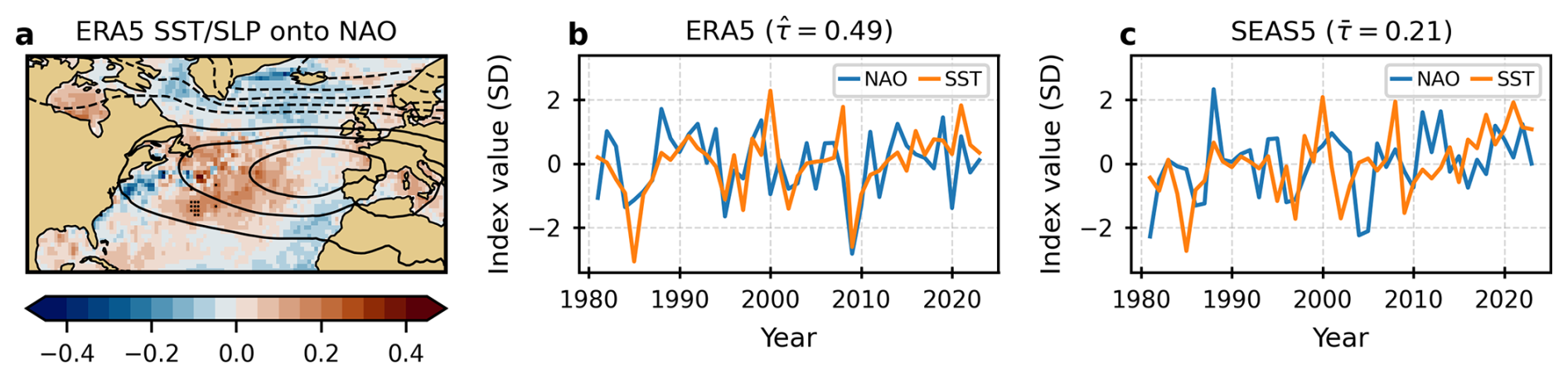
Figure 1 (a) Colours: November SST anomalies in ERA5 projected onto the ERA5 DJF NAO index. The unit is K, and dots mark coefficients significantly different from zero at the 5 % level. Contours: DJF SLP anomalies projected onto the same NAO index (unit: hPa). The contour interval is 1 hPa; solid (dashed) contours indicate positive (negative) coefficients, and the zero contour is omitted. The map extent corresponds to the region used to define the November SST index. (b) Time series of the November SST index (orange) and the DJF NAO index (blue) in ERA5. Years on the x-axis correspond to the December month at the start of the winter (i.e. DJF 1981/82 is labelled 1981). (c) As in (b), but for SEAS5, based on the ensemble mean each year.

Figure 1b shows the interannual November SST index, obtained by projecting the SST anomalies onto the regression pattern in Fig. 1a, together with the winter NAO index, both from ERA5 data. Although only a few of the local SST coefficients in Fig. 1a are significant, the sample correlation between the two indices is relatively high ($\widehat{\mathit{\tau }}=\mathrm{0.49}$, p≈0.001), underscoring the strong link between late-autumn SSTs and the subsequent winter NAO. The SST index captures well the two exceptionally negative NAO winters of 2009/10 and 2010/11, as well as the extended positive NAO phase around 1990, though there are also seasons with weak correspondence, such as 2000/01. It is emphasised that $\widehat{\mathit{\tau }}$ does not represent a skill score, as no independent training and evaluation periods were defined.

Turning to the (ensemble mean) SEAS5 indices shown in Fig. 1c, it is evident that the SST index covaries with the SST index in ERA5 (r=0.91). However, several differences between the datasets are also apparent. Most important, the SST–NAO correlation is substantially lower ($\stackrel{\mathrm{‾}}{\mathit{\tau }}=\mathrm{0.21}$, p=0.18, with the overbar signifying that the ensemble mean was used) than in ERA5, demonstrating a discrepancy in the linkages between the observed “NAO-optimal” SST pattern and the winter NAO. Here it is acknowledged that the SST–NAO correlation is weaker than in ERA5 at least partly because both indices were deliberately derived from ERA5-based spatial patterns.

A second point is the non-significant NAO skill: the anomaly correlation coefficient between the NAO index in SEAS5 and ERA5, denoted henceforth as ρ, is not significant for the ensemble mean ($\stackrel{\mathrm{‾}}{\mathit{\rho }}=\mathrm{0.29}$, p=0.06). This low predictive power is consistent with Baker et al. (2024).

When the SST–NAO correlation and the NAO skill are evaluated for all the ensemble members instead of for the ensemble mean, both metrics deteriorate, revealing higher internal noise. This behaviour is consistent with the “signal-to-noise paradox” (e.g. Scaife and Smith, 2018). The sample parameter based on all members, which is used in the remainder of the analysis, is $\widehat{\mathit{\tau }}=\mathrm{0.06}$, which is not significantly positive and much lower than $\stackrel{\mathrm{‾}}{\mathit{\tau }}=\mathrm{0.21}$. The member-level NAO skill also decreases from $\stackrel{\mathrm{‾}}{\mathit{\rho }}=\mathrm{0.29}$ to the non-siginificant value of $\widehat{\mathit{\rho }}=\mathrm{0.07}$.

4.2 Linking the SST–NAO relationship to NAO prediction skill

One of the three main purposes of this paper is to assess whether the total SST–NAO relationship (τ in Eq. 1) in the model is proportional to its NAO skill. That skill is defined here as ρ: the correlation between the DJF NAO index in SEAS5 and the corresponding DJF NAO index in ERA5, with ERA5 years selected to match the year of each SEAS5 member. If there had been no relationship between τ and ρ, it would be of limited interest to scrutinise the causal pathways through which the SSTs influence the NAO.

It is important to emphasise that ρ is an external quantity: it depends solely on the correlation between the SEAS5 and ERA5 DJF NAO indices and contains no information about the model’s internal relationships among X, Z, and Y. By contrast, the total effect τ and the mediated effect αβ derive entirely from SEAS5’s internal covariance structure. There is therefore no algebraic or definitional link between skill and any aspect of the model’s SST–NAO relationship. Any association between the two reflects actual co-variation between an external validation measure and internal model dynamics, rather than an outcome expected by construction.

To investigate the association between τ and ρ, bootstrapping was used to generate an ensemble of 10 000 SEAS5 series, each with the same length as the number of years in the study period (43). The results are not sensitive to this choice of length, and the same bootstrap ensemble is analysed further in Sect. 4.6.

For each bootstrap series, two quantities were computed: (1) $\widehat{\mathit{\tau }}$, the sample SEAS5-internal correlation between the November SST index and the DJF NAO index; and (2) $\widehat{\mathit{\rho }}$, the sample NAO skill. Figure 2 shows a scatterplot of these parameters for a subset of the series. The correlation across all the 10 000 series is positive (r=0.33) and significant at the 5 % level. This does not imply that a strong SST–NAO relationship is sufficient or strictly required for high NAO skill, since the NAO is influenced by many processes unrelated to North Atlantic SST variability. Rather, the result provides support for a central premise of this study: the extent to which the model reproduces the observed influence of November SST anomalies on the winter NAO contributes meaningfully to its overall NAO skill.

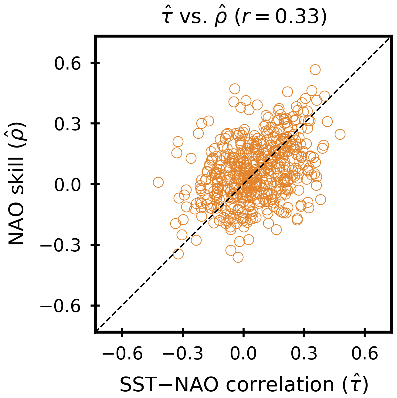
Figure 2 Results for a 10 000-member bootstrap ensemble of SEAS5 series, each of length 43. For each bootstrap sample, the x-axis shows the SEAS5-internal correlation between the November SST index and the DJF NAO index, and the y-axis shows the NAO skill $\widehat{\mathit{\rho }}$, defined as the correlation between the DJF NAO indices in SEAS5 and ERA5 (with ERA5 years matched to the bootstrap sample). To enhance readability, only 1000 randomly chosen points are shown.

4.3 ERA5 climatology and SEAS5 bias

Before examining the role of SHF and baroclinicity in mediating the SST–NAO relationship, it is useful to consider the climatological context. In Fig. 3, ERA5 climatologies and SEAS5 biases are therefore shown, starting with the mean November SSTs in the North Atlantic in Fig. 3a. A prominent feature is the strong SST gradient along the boundary between the warm Gulf Stream waters and the much colder waters along the North American coastline. These gradients give rise to intense SHF on the warm side of the front (Fig. 3b), and they also coincide with strong low-level baroclinicity (Fig. 3c). The last panel in the top row, Fig. 3d, shows the climatological SLP pattern, which is characterised by a dipole between the Icelandic Low and the Azores High.

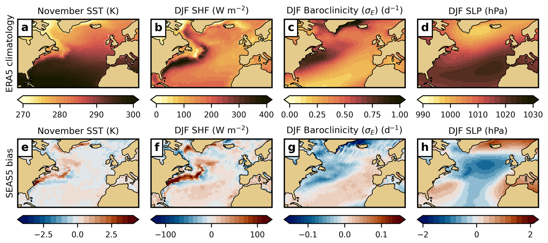
Figure 3 Top row (a–d): ERA5 climatologies for (a) November SST (K); (b) DJF surface heat fluxes (W m⁻²); (c) DJF Eady growth rate maximum σ_E (d⁻¹); (d) DJF SLP (hPa). The bottom row (e–h) show the SEAS5 biases (SEAS5 minus ERA5) for the same variables as in the top row.

The aforementioned warm SST bias in the western North Atlantic (Stockdale et al., 2018; Tietsche et al., 2020) is visible as a tongue-like feature in the east–west direction south of Greenland in Fig. 3e. This is also linked to a clearly defined positive DJF SHF bias in Fig. 3f. The poor SEAS5 representation of the SST gradient along the Gulf Stream seen in Fig. 3a is also of interest. Figure 3e reveals a pronounced warm bias on the cold side of the front and a weaker cold bias on the warm side, resulting in an overall weakened gradient. The SHF biases in Fig. 3f reflect these SST errors, generally showing fluxes that are too strong in warm-biased regions and too weak in cold-biased sectors. Although not shown here, these SHF biases project strongly onto the DJF SST bias in the western part of the basin; these are larger in magnitude than the ones for November in Fig. 3e, but for the most part they have the same sign, suggesting a growth of the model's SST bias with lead time. Figure 3g indicates that the underestimated SST gradients along the Gulf Stream are associated with too weak baroclinicity in the storm track entrance region, while σ_E is too high to the south.

These errors imply a distorted storm track: too few cyclones over the northern North Atlantic and too many further south, which is consistent with the IFS cyclone bias investigations by Jung et al. (2006) and Büeler et al. (2024). This interpretation is supported by the mean SLP bias pattern in Fig. 3h, which shows that SEAS5 underestimates the amplitude of the observed NAO-like dipole. Sampled at representative grid points near the two NAO centres of action (Stykkishólmur, Iceland, and Ponta Delgada, Azores), the mean SLP bias amounts to +1.0 and −0.4 hPa, respectively, giving a bias in the north–south difference of +1.4 hPa. This confirms that the model’s climatological pressure contrast is weaker than observed, implying westerlies that are too weak across the subpolar North Atlantic. The most distinct weakening of the westerlies occurs between the mid-basin negative SLP bias and the positive bias near Iceland. This corresponds to the weak negative SHF bias observed in the same region (Fig. 3f). In this area with suppressed westerlies, surface fluxes are likely underestimated because reduced wind speeds dampen the intensity of the cold-air advection from the west.

4.4 Mediated effects

Figures 4 and 5 show the sample parameters $\widehat{\mathit{\alpha }}$ and $\widehat{\mathit{\beta }}$, as well as their product $\widehat{\mathit{\alpha }}\widehat{\mathit{\beta }}$, for both mediators. The unit is standard devations (SD), as all the variables in the regression equations were standardised prior to estimating the coefficients. It is repeated for emphasis that α, the regression coefficient linking November SSTs to the mediator (X→Z) in Eq. (3), captures all routes through which SST anomalies influence Z. This includes the indirect effect via the NAO (i.e. the pathway $X\to Y\to Z$), as well as other pathways not explicitly considered here. The NAO-independent contribution of SSTs to Z, denoted α^′ in Eq. (5), is examined in Sect. 4.5.

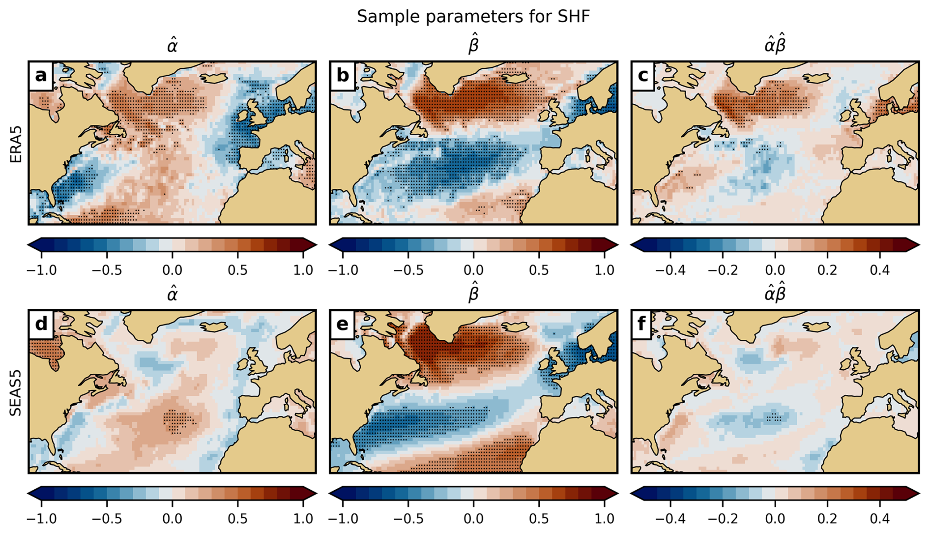
Figure 4 The top row shows sample parameters for ERA5 for the surface heat flux pathway: (a) $\widehat{\mathit{\alpha }}$; (b) $\widehat{\mathit{\beta }}$; (c) the mediated effect ($\widehat{\mathit{\alpha }}\widehat{\mathit{\beta }}$). Panels (d)–(f) show the corresponding parameters for SEAS5. Dots indicate where the parameters differ significantly from zero at the 5 % level. Unit in all panels: standard deviations (SD).

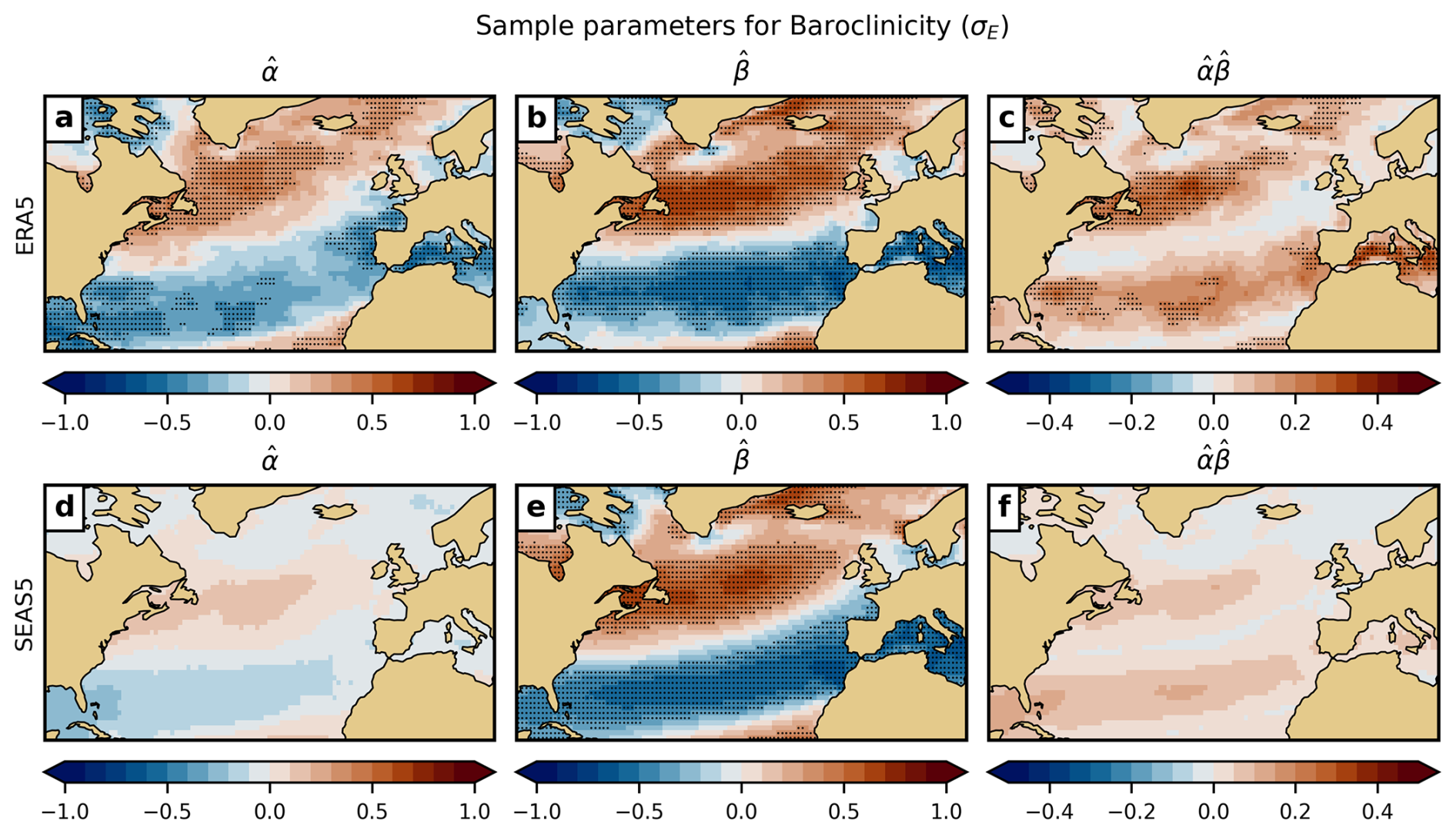
Figure 5 As Fig. 4, but for the baroclinicity parameter σ_E.

4.4.1 Surface heat fluxes

From Fig. 4a, it emerges that the November SST index yields positive SHF coefficients in large parts of the Subpolar Gyre in ERA5. These positive $\widehat{\mathit{\alpha }}$ values largely coincide with positive $\widehat{\mathit{\beta }}$ values (Fig. 4b). The product $\widehat{\mathit{\alpha }}\widehat{\mathit{\beta }}$ therefore yields a pronounced mediated effect in the reference region (Fig. 4c), consistent with Kolstad and O'Reilly (2024). This implies that heat fluxes in this area play an important role in mediating the effect of November SSTs on the winter NAO.

Limited suppression occurs in the mid-basin area, suggesting a negative feedback mechanism. This happens because $\widehat{\mathit{\alpha }}$ and $\widehat{\mathit{\beta }}$ have opposing signs; in other words, the SST index generates a flux response that counteracts the contemporaneous NAO–SHF relationship.

Figure 4d reveals that SEAS5 yields barely any significant $\widehat{\mathit{\alpha }}$ values. Although there is a fair degree of spatial correspondence with the findings for ERA5, the uniformly positive structure south of Greenland seen in the reanalysis is lacking. Instead, $\widehat{\mathit{\alpha }}$ is partly negative; this roughly overlaps with the positive SST and SHF biases identified in Fig. 3e, f. The spatial match is not exact, however, and there is no obvious mechanistic link between the bias and the sign reversal. Regardless of its origin, the model produces the wrong sign of the SST-flux relationship in a dynamically important region, in marked contrast to ERA5.

In comparison, the pattern of $\widehat{\mathit{\beta }}$ (Fig. 4e) does resemble the one in ERA5, demonstrating that SEAS5 has a strong and mainly correct contemporaneous SHF–NAO relationship. However, the mediated effect $\widehat{\mathit{\alpha }}\widehat{\mathit{\beta }}$ in SEAS5 shown in Fig. 4f diverges from ERA5, with no significant mediation in the Subpolar Gyre region. In light of the strong $\widehat{\mathit{\beta }}$ pattern, this suggests that the SHF-related part of this weak SST–NAO correlation is due to the inadequate $\widehat{\mathit{\alpha }}$ representation. This is discussed further in Sect. 4.5.

Lastly, it is noteworthy that SEAS5 exhibits suppression in the same mid-basin domain as ERA5.

4.4.2 Baroclinicity

The top row of Fig. 5 (panels a–c) shows a distinctly positive mediated effect in ERA5 in the western storm track entrance region, in a wide corridor further south, and near Iceland. In all these areas, the sign of $\widehat{\mathit{\alpha }}$ and $\widehat{\mathit{\beta }}$ is the same, and the spatial structures of these parameters are similar. This likeness could indicate that the mediated effect is mainly due to the effect of the NAO on the baroclinicity (i.e. Y→Z). In that case, $\widehat{{\mathit{\alpha }}^{\prime }}$ in Eq. (5) is expected to be near-zero; this is explored in the next section. Even so, feedbacks between the NAO and baroclinicity (i.e. eddy-mean flow feedbacks) still appears to be an important mechanism for maintaining the NAO.

The picture for SEAS5 (Fig. 5d–f) is similar to ERA5 in the sense that the signs of $\widehat{\mathit{\alpha }}$ and $\widehat{\mathit{\beta }}$ overlap in two bands across the North Atlantic. However, the magnitude of $\widehat{\mathit{\beta }}$ is distinctly larger than that of $\widehat{\mathit{\alpha }}$; clearly the magnitude of the muted mediated effect in panel (f) is dictated by $\widehat{\mathit{\alpha }}$. Neither $\widehat{\mathit{\alpha }}$ nor $\widehat{\mathit{\alpha }}\widehat{\mathit{\beta }}$ is significant anywhere.

4.5 Disentangling forcing and feedback

The findings in the previous section raised questions about the directionality of the mediated effects associated with both SHF and baroclinicity. Although the pathway $X\to Z\to Y$ is not meant to be interpreted as strictly unidirectional, evaluating the X→Z link in isolation helps determine the extent to which November SST anomalies generate responses independently of the NAO. To that end, the leftmost panels in Fig. 6 show the sample parameter $\widehat{{\mathit{\alpha }}^{\prime }}$ from Eq. (5), which isolates the X→Z influence with the NAO regressed out, for SST and SLP. These variables, which are not considered as mediators, are analysed here because they indicate changes in the lower boundary (SST) and circulation (SLP).

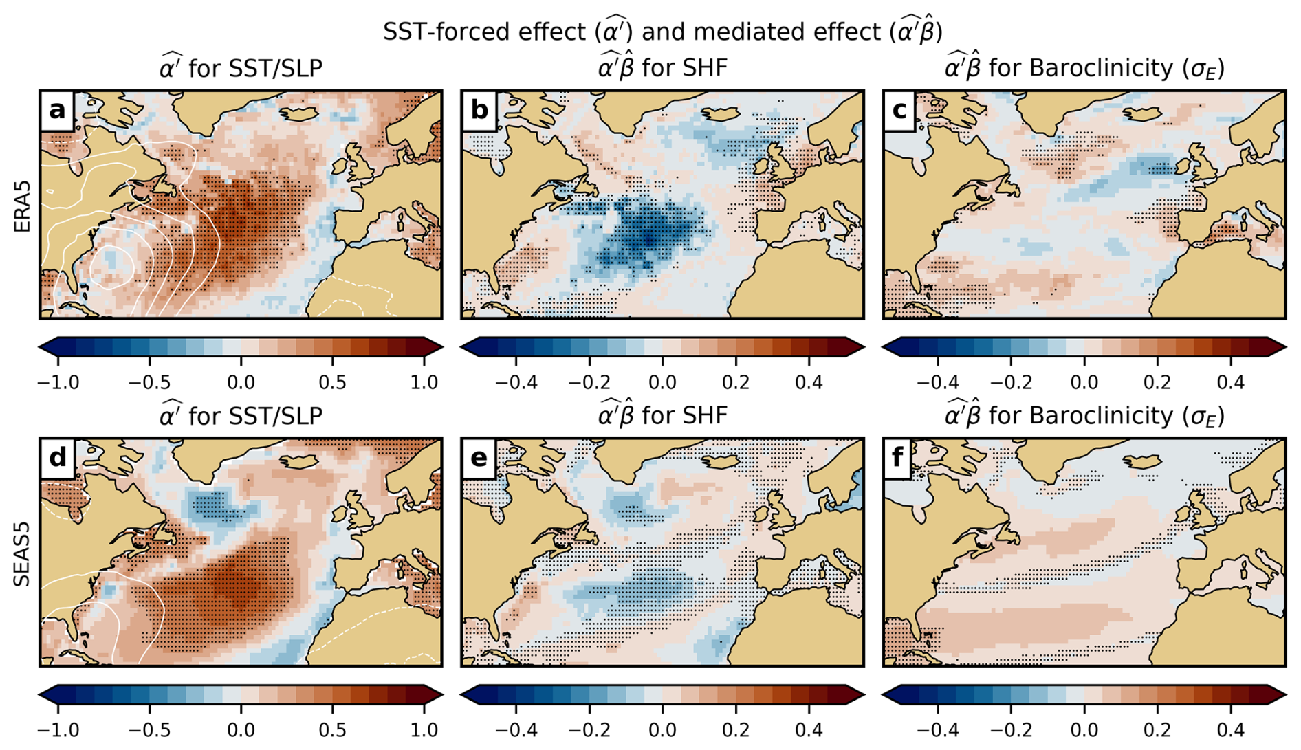
Figure 6 The left column shows the November SST-forced effect ($\widehat{{\mathit{\alpha }}^{\prime }}$; Eq. 5), on DJF SST (colours) and SLP (contours with interval 0.1 SD; positive solid, negative dashed; zero omitted) in ERA5 (a) and SEAS5 (d). Dots indicate where $\widehat{{\mathit{\alpha }}^{\prime }}$ for SST is significantly different from zero at the 5 % level. The remaining panels show the November SST-forced mediated effect ($\widehat{{\mathit{\alpha }}^{\prime }}\widehat{\mathit{\beta }}$) on ERA5 SHF (b), ERA5 baroclinicity (c), SEAS5 SHF (e), and SEAS5 baroclinicity, all in DJF. Dots denote where the ratio $\widehat{{\mathit{\alpha }}^{\prime }}/\widehat{\mathit{\alpha }}$ is significantly positive at the 5 % level.

Starting with ERA5, Fig. 6a shows that, once the NAO contribution is removed, November SST anomalies induce an SLP pattern dominated by positive coefficients over the south-western North Atlantic. This pattern implies anomalous northerly advection in positive phases and southerly advection in negative phases. The associated SST response resembles the November antecedent in Fig. 1a (as expected from oceanic inertia), but there is more pronounced mid-basin dominance with positive values.

In SEAS5, the $\widehat{{\mathit{\alpha }}^{\prime }}$ field in Fig. 6d shows an SST structure broadly similar to the ERA5 pattern in panel (a), with one notable exception: significant negative values appear south of Greenland. A similar sign discrepancy was already seen for the SHF $\widehat{\mathit{\alpha }}$ coefficient (Fig. 4d), indicating that the SST–flux response in this region is systematically misrepresented in SEAS5. These negative $\widehat{{\mathit{\alpha }}^{\prime }}$ values lie near the well-documented positive SST bias during the early reforecast period (Stockdale et al., 2018; Tietsche et al., 2020), and when the analysis is repeated for 2001–2023, when this bias was much smaller, the negative values largely disappear. This suggests that the sign error may be linked to compensating adjustments associated with the bias, although the spatial correspondence is not exact and the mechanism cannot be established here. However, this issue is not central to the present study – while the bias alters some spatial details in SEAS5, the mediated effect in SEAS5 is not significant in this region in either period, and the skill–mediation covariability discussed in Sect. 4.6 is unaffected.

The SST-forced mediated effect $\widehat{{\mathit{\alpha }}^{\prime }}\widehat{\mathit{\beta }}$ via surface heat fluxes in ERA5 is shown in Fig. 6b. In this panel the dots indicate areas where the null hypothesis – that α^′ and α have opposite signs – can be rejected at the 5 % level across the 10 000 bootstrap samples. In these areas the SST-forced component contributes in the same direction as the full mediated effect, which includes contemporaneous feedbacks from the NAO onto the fluxes. Over parts of the Subpolar Gyre, where β is positive (Fig. 4b), $\widehat{{\mathit{\alpha }}^{\prime }}\widehat{\mathit{\beta }}$ is partly positive or near-neutral, but few areas are marked with dots. This indicates that the strong total mediation seen in Fig. 4c is largely attributable to the Y→Z pathway; that is, NAO feedbacks on the fluxes dominate in this region. Further south in the North Atlantic, $\widehat{{\mathit{\alpha }}^{\prime }}\widehat{\mathit{\beta }}$ is negative over a broad area. The density of dots there indicates that the NAO-independent SST-forced component contributes to suppressing the SST–NAO correlation. A similar but less extensive pattern appears in the full mediated effect $\widehat{\mathit{\alpha }}\widehat{\mathit{\beta }}$ in Fig. 4c.

In SEAS5 (Fig. 6e), the spatial structure of $\widehat{{\mathit{\alpha }}^{\prime }}\widehat{\mathit{\beta }}$ resembles the pattern of the full mediated effect $\widehat{\mathit{\alpha }}\widehat{\mathit{\beta }}$ in Fig. 4c. Some areas are marked with dots, including the mid-basin region exhibiting suppression. This implies that the SST-forced component plays a role in this suppression, matching the ERA5 result in Fig. 6b.

For baroclinicity, Fig. 6c shows that the SST-forced mediated effect is mainly positive in the two bands where the total mediated effect $\widehat{\mathit{\alpha }}\widehat{\mathit{\beta }}$ is positive and significant (Fig. 5c), albeit noticeably weaker in magnitude. Parts of these bands are marked with dots, indicating where the SST-forced component plays a limited role in the full mediation. Figure 6f demonstrates that SEAS5 similarly produces weak, positive $\widehat{{\mathit{\alpha }}^{\prime }}\widehat{\mathit{\beta }}$ in the two bands, but no dots appear where the mediated effect is strongest in magnitude. This suggests that the SST-driven component of the mediated effect in the crucial areas is negligible.

In summary, the directional picture is heterogeneous but broadly consistent with a dominant NAO → mediator pathway. For SHF, the SST-driven contribution mainly projects onto the mid-basin area where suppression dominates, while over parts of the Subpolar Gyre the strong total mediation appears to be largely attributable to NAO feedbacks onto the fluxes. For baroclinicity, ERA5 indicates a modest SST-forced contribution aligned with the total response in two bands – albeit noticeably weaker than the full mediation – whereas SEAS5 shows no such contribution. These results motivate the next step: to assess whether variations in these internally generated mediation patterns are associated with variations in external NAO forecast skill.

4.6 Relating mediated effects to NAO prediction skill

In Sect. 4.2, a modest but significant association was identified between the November-to-DJF SST–NAO correlation and the model's NAO skill $\widehat{\mathit{\rho }}$ (r=0.33). This suggests that the mediated effect associated with the SST–NAO linkage may also relate to forecast skill. Although the mediation signal in SEAS5 is weak overall, it is not absent: the positive $\widehat{\mathit{\alpha }}\widehat{\mathit{\beta }}$ values for baroclinicity (Fig. 5f) broadly overlap with those in ERA5 (Fig. 5c). For SHF (Fig. 4c, f), there is likewise some agreement, apart from the negative values south of Greenland noted earlier.

This section examines whether variations in mediation strength across subsets of SEAS5 realisations are associated with variations in NAO skill. To do so, the 10 000-member bootstrap ensemble introduced in Sect. 4.2 is revisited. For each bootstrap sample, the SEAS5 mediated effect $\widehat{\mathit{\alpha }}\widehat{\mathit{\beta }}$ is estimated separately for SHF and σ_E, alongside the NAO skill $\widehat{\mathit{\rho }}$ and the model-internal SST–NAO correlation from Sect. 4.2.

The maps in Fig. 7 show where, geographically, the mediated effect $\widehat{\mathit{\alpha }}\widehat{\mathit{\beta }}$ co-varies with the NAO skill $\widehat{\mathit{\rho }}$ across the SEAS5 bootstrap samples. The most prominent feature is that the strongest positive correlations occur in the regions where ERA5 exhibits robust positive mediation. For SHF (Fig. 7a), this positive covariability appears across the Subpolar Gyre, even south of Greenland, where the overall $\widehat{\mathit{\alpha }}\widehat{\mathit{\beta }}$ in SEAS5 is negative (Fig. 4f). This indicates that, within SEAS5, bootstrap subsets in which the model produces a mediation pattern more closely resembling ERA5 are also the subsets with higher NAO skill. Conversely, samples that yield negative $\widehat{\mathit{\alpha }}\widehat{\mathit{\beta }}$ in these regions tend to have lower skill. Thus, even though SEAS5 does not reproduce the magnitude or sign of the mediated effect perfectly, its internal covariability shows that more realistic mediation pathways are associated with improved NAO prediction skill.

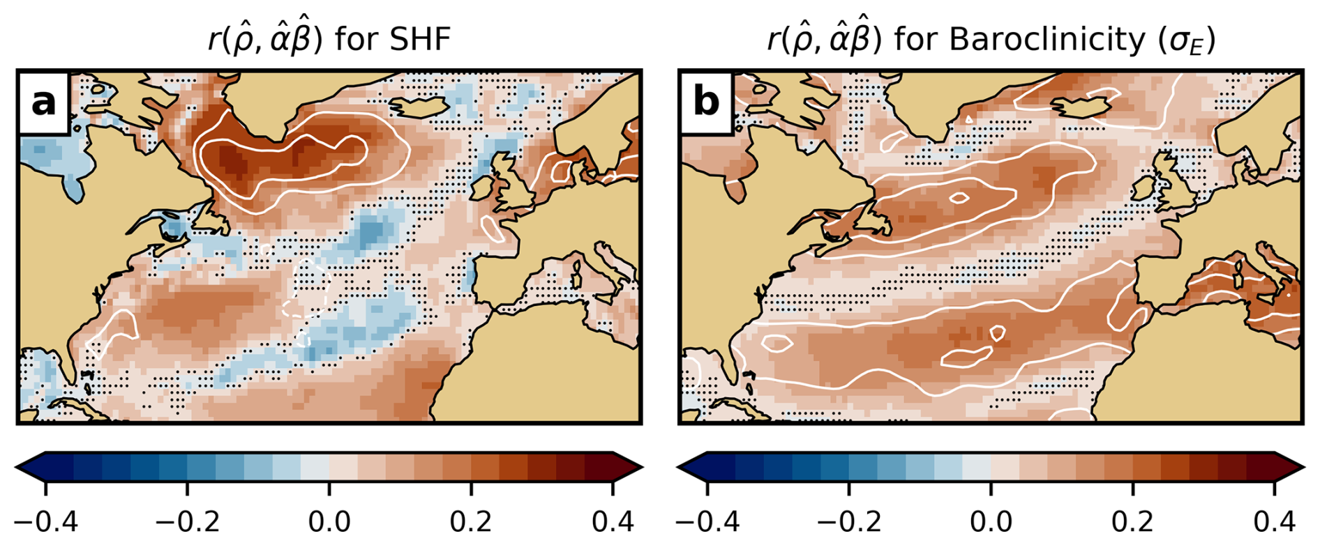
Figure 7 Results for the 10 000 bootstrap samples introduced in Sect. 4.2. Shading shows the correlation between $\widehat{\mathit{\rho }}$ and the mediated effect $\widehat{\mathit{\alpha }}\widehat{\mathit{\beta }}$, computed from SEAS5 for each bootstrap sample, for (a) surface heat fluxes (SHF) and (b) baroclinicity. Dots indicate correlations that do not significantly differ from zero at the 5 % level. White contours reproduce the ERA5 mediated effect $\widehat{\mathit{\alpha }}\widehat{\mathit{\beta }}$ from Figs. 4c and 5c in panels (a) and (b), respectively (contour interval 0.1 SD; positive solid, negative dashed; zero omitted).

A few regions also display negative correlations between $\widehat{\mathit{\rho }}$ and $\widehat{\mathit{\alpha }}\widehat{\mathit{\beta }}$, but these do not overlap with the key regions where ERA5 exhibits strong SHF-mediated effects in the Subpolar Gyre. For baroclinicity, the correspondence between $\widehat{\mathit{\rho }}$ and $\widehat{\mathit{\alpha }}\widehat{\mathit{\beta }}$ is more uniformly related to the mediated effect in ERA5 (Fig. 7b).

Taken together, these patterns reinforce the main conclusion: the clearest and most physically interpretable skill-mediation covariability occurs in the regions where ERA5 displays robust positive mediation. In these areas, SEAS5 achieves higher NAO skill when it incidentally reproduces the observed mediation pathways, underscoring the importance of representing these air–sea feedbacks realistically in seasonal prediction systems.

As noted in Sect. 4.2, the skill and mediation metrics derive from entirely different sources of information. The fact that they co-vary in physically meaningful regions therefore supports the view that the ERA5-identified pathways correspond to mechanisms that matter for NAO predictability in the model.

5 Summary and discussion

In this paper, feedback pathways linking the state of the North Atlantic sea surface in late autumn and the NAO during the following winter have been explored. As in Kolstad and O'Reilly (2024), these pathways were investigated using mediation analysis, a branch of statistical causal inference methods that has seen little use in climate dynamics so far. The results demonstrate that feedbacks previously identified through idealised perturbation experiments in dynamical models can also be diagnosed directly from observational or reanalysis data. One advantage of this approach is that it avoids the need to manipulate boundary conditions like SSTs. Such manipulations can elicit compensatory model adjustments that complicate interpretation, particularly when the models themselves suffer from systematic biases. Mediation analysis instead infers causal structure directly from observed covariability, offering a complementary perspective on internal feedback pathways.

It must nevertheless be acknowledged that reanalysis products are themselves produced with models – in the case of ERA5, from the same model lineage as SEAS5. Thus, reanalyses are not free from biases, and their depiction of physical relationships may be influenced by model behaviour. Mediation analysis cannot fully resolve such issues, but by contrasting reanalysis-based and model-based feedbacks, it can help to pinpoint where key processes diverge.

Additional limitations should be kept in mind. For one, the mediation framework as applied here is linear and does not adequately capture nonlinear feedbacks. Further, SEAS5 is only one dynamical system; different models likely represent feedback differently. Future work could extend this examination to other models, some of which exhibit higher NAO skill than SEAS5 (Baker et al., 2024), or indeed multi-model ensembles, incorporating nonlinear mediation analysis techniques. Another limitation is that the analysis does not condition on remote precursors. For instance, ENSO can influence both late-autumn North Atlantic SSTs and the winter NAO, potentially giving rise to apparent, but non-causal, links between pre-winter SST and the NAO. An idea for future research could be to extend the framework by explicitly conditioning on, or stratifying by, for instance tropical predictors or stratosphere–troposphere interactions.

Notwithstanding these caveats, this study has extended Kolstad and O'Reilly (2024), where processes linking late‐autumn SST anomalies and the winter NAO were analysed based on ERA5 data, by investigating these processes in the forecast system SEAS5. It was hypothesised that the SST–NAO relationship has bearing on the NAO prediction skill in that model, and this was confirmed. Although the observed correlation (r=0.33) is modest, it still represents a non-trivial association in light of the many other processes that influence NAO skill, including the stratosphere, tropical SST variability, Arctic sea‐ice anomalies, and internal atmospheric dynamics, to mention but a few.

Having established this link between the SST–NAO relationship and NAO skill, the analysis extended Kolstad and O'Reilly (2024) further by revealing a physically coherent sequence of processes underpinning the SST–NAO connection. Independently of the NAO, November SST anomalies induce a surface‐pressure pattern that preconditions the atmosphere for anomalies in two mediators: surface heat flux (SHF) and baroclinicity in the western North Atlantic. These anomalies in turn nudge the NAO, which subsequently feeds back on both SHF and baroclinicity. A key outcome concerns the directionality of these causal pathways. Across large parts of the North Atlantic, forcing from the NAO onto the mediators was found to dominate. Crucially, however, in the regions with the strongest mediated effects through SHF and baroclinicity, the directionality was ambiguous, consistent with the existence of a two-way feedback mechanism.

It is important to emphasise that these feedbacks do not account for all aspects of NAO variability. The processes identified here represent one pathway among many, complementing the aforementioned influences from, for example, the stratosphere. Rather than providing a complete explanation, the results demonstrate how even a single coupled feedback sequence can shape NAO variability and how its misrepresentation in a prediction system may limit its ability to capture the full range of NAO behaviour.

A key finding is that these pathways are substantially weakened in SEAS5. This is likely linked to the muted SST–NAO relationship in the model relative to ERA5. When this link is weak, the total effect of SSTs on the mediators, labelled α herein, is also necessarily weak. Figure 7, where bootstrap resampling was used to explore the relationship between NAO prediction skill and the mediated SST–NAO effect, illustrates this succinctly. Model samples that exhibit a stronger mediated effect also show higher NAO prediction skill. Conversely, samples that by chance yield higher NAO skill also display a stronger mediated effect. This mutual dependence suggests that if the model were able to reproduce the SST–NAO pathways via SHF and baroclinicity more realistically, it would likely predict the NAO more accurately as well.

However, this counterfactual hypothesis cannot be tested directly because the model does not currently reproduce these pathways. Targeted experiments that enforce more realistic air-sea interactions could help clarify whether strengthening these pathways would indeed improve NAO prediction skill. The study by Roberts et al. (2021) provides a prime example of such experiments. Other improvements, such as enhancing the resolution of the ocean (e.g. Haarsma et al., 2019) or the atmosphere (e.g. Czaja et al., 2019; Wills et al., 2024), or improving the representation of eddy–mean flow feedbacks (e.g. Hardiman et al., 2022), have also been shown to produce more precise atmospheric responses to SST forcing.

The results presented here raise interesting questions for the emerging class of ML-based seasonal and subseasonal prediction systems (e.g. Chen et al., 2024; Kent et al., 2025). If trained on model-generated data or on reanalyses influenced by model biases, such systems risk inheriting some of the deficiencies documented here. Conversely, ML approaches trained directly on observations might bypass some of these problems – but whether they would be able to capture the same preconditioning and feedback structures as the real climate system is currently unknown.

Mediation analysis offers a powerful and versatile framework for tackling these research challenges. It can help pinpoint where models fail to represent key causal pathways, assess whether targeted improvements translate into more realistic coupled feedbacks and higher predictive skill, and evaluate whether ML-based forecasts reproduce the same physical linkages observed in nature. In a broader sense, mediation analysis can serve as a bridge between statistical diagnostics and both process studies and model development/evaluation, advancing our understanding of how both unidirectional and feedback mechanisms shape climate predictability.