Flow dependence of wintertime subseasonal prediction skill over Europe

Issuing skillful forecasts beyond the typical horizon of weather predictability remains a challenge actively addressed by the scientific community. This study evaluates winter subseasonal reforecasts delivered by the CNRM and ECMWF dynamical systems and identifies that the level of skill for predicting temperature in Europe varies fairly consistently in both systems. In particular, forecasts initialized during positive North Atlantic Oscillation (NAO) phases tend to be more skillful over Europe at week 3 in both systems. Composite analyses performed in an atmospheric reanalysis, a long-term climate simulation and both forecast systems unveil very similar temperature and sea-level pressure patterns 3 weeks after NAO conditions. Furthermore, regressing these fields onto the 3-weeks-prior NAO index in a reanalysis shows consistent patterns over Europe but also other regions of the Northern Hemisphere extratropics, thereby suggesting a lagged teleconnection, related to either the persistence or recurrence of the positive and negative phases of the NAO. This teleconnection, conditioned to the intensity of the initial NAO phase, is well captured by forecast systems. As a result, it is a key mechanism for determining a priori confidence in the skill of wintertime subseasonal forecasts over Europe as well as other parts of the Northern Hemisphere.

1 Introduction

Skillful weather and climate predictions for horizons beyond 2 weeks could benefit many users (White et al., 2017). Lately, so-called subseasonal-to-seasonal (S2S) forecasts have gained considerable attention and effort from the scientific community in multiple aspects, including the characterization of sources of predictability, such as atmospheric teleconnections, the initialization and generation of ensemble forecasts, the calibration and tailoring of the raw model outputs for enhanced usability, and uptake by the application community (Merryfield et al., 2020). The S2S horizon has been often considered to be a “predictability desert” based on mean statistics and traditional methods and analyses inspired from seasonal to decadal climate prediction, but the most recent studies reveal instead so-called windows of opportunity based on the fact that under certain circumstances and for specific events and regions, S2S predictability can be considerably increased (Mariotti et al., 2020). This conditional predictability is illustrated by a number of case studies showing the successful anticipation of extreme climate events by dynamical forecast systems beyond 15 d lead time (Domeisen et al., 2021). Rather than a predictability desert, the S2S horizon appears more like a “predictability well” intermittently fed by these windows of opportunity. Timely drawings from the well, i.e., a priori identification of the windows of opportunity, are a major asset in an operational context for the development and uptake of climate services relying on subseasonal forecasts, but it remains a scientific challenge with some promising examples. For instance, Mayer and Barnes (2021) recently related the accuracy of North Atlantic geopotential height forecasts issued by a neural network to their level of confidence. Their approach also allows the most relevant remote tropical regions to be pinpointed, leading to higher forecast skill.

At the subseasonal scale, European and eastern North American climate is influenced by the phase of the North Atlantic Oscillation (NAO), the leading mode of climate variability over the North Atlantic sector (Cattiaux et al., 2010; Seager et al., 2010; Luo et al., 2020). The positive (NAO+) and negative (NAO-) phases of the NAO correspond to two well-identified weather regimes characterizing recurrent synoptic-scale atmospheric patterns in winter, along with the Atlantic Ridge (AR) and Scandinavian blocking (BLO) (e.g., Vautard, 1990). The NAO is sometimes considered to be the local manifestation of a hemispheric variability pattern called Northern Annular Mode or Arctic Oscillation (AO). AO and NAO are strongly correlated in present climate (Hamouda et al., 2021).

The tropics–extratropics teleconnection described by Cassou (2008) and Lin et al. (2009) illustrates the major role of the Madden–Julian Oscillation (MJO) phase in pre-conditioning North Atlantic weather regimes. Recently, Lee et al. (2019) found evidence of El Niño–Southern Oscillation (ENSO) modulating the strength of this teleconnection which largely contributes to the subseasonal predictability of the North Atlantic (Vitart, 2017). More generally, the tropical background state and variability are essential to induce subseasonal predictability of the Northern Hemisphere circulation, especially in winter, provided that the climate phenomena supporting the teleconnection, such as the atmospheric upper-level jet, are adequately simulated (Yamagami and Matsueda, 2020). The stratosphere is another key precursor to the variability and predictability of the wintertime Northern Hemisphere circulation (Domeisen et al., 2020). A correct initialization (Zuo et al., 2016), together with a good representation of the stratosphere–troposphere coupling (Kolstad et al., 2020), accordingly contributes to the skillful forecast of the NAO. The combination of ENSO evolution and stratospheric processes also drives the extended-range NAO predictability (Sun et al., 2020).

Other studies have focused on the predictability conditioned by the wintertime weather regimes occurring at initialization time. Based on a specific set of weather regimes affecting North America, Vigaud et al. (2018) demonstrated the capacity of the ECMWF subseasonal forecast system to successfully predict some of them up to 2 weeks. Robertson et al. (2020) built on this study to emphasize the value of this weather regime approach for identifying forecasts of opportunity over North America, with high skill up to 30 d ahead for specific events or seasons. The flow-dependent variations in the subseasonal forecast skill over Europe were also evidenced (Ferranti et al., 2018), with a relatively good capacity of the ECMWF system to reproduce the preferred transitions between weather regimes. Ferranti et al. (2015) identified differences in medium-range weather forecast performances conditional to the regime flow in the initial conditions with initial NAO- states leading to more skillful forecasts. Beyond approaches based on weather regime prediction, Minami and Takaya (2020) recently found that Northern Hemisphere 500 hPa geopotential height was more predictable when following strong negative initial AO due to an eddy-zonal flow feedback that contributes to the persistence of this mode of atmospheric variability. This study emphasizes the role played by large-scale extratropical atmospheric dynamics in subseasonal predictability on top of tropical and stratospheric precursors.

Our main goal here is to further explore the relationship between the circulation flow present in the forecast initial conditions, hereafter initial weather regimes, and subseasonal predictability of the 2 m temperature in winter over a broad North Atlantic European domain. In this study we analyze jointly the ECMWF forecast system and the most recent CNRM (Météo-France) subseasonal forecast system, launched in October 2020. The next section presents these forecast systems as well as reference data and methods adopted in this study. The main results are then developed in a dedicated section. The last section provides concluding remarks and prospects.

2 Data and methods

2.1 Forecast systems

Subseasonal forecasts delivered by CNRM have been routinely feeding the S2S database (Vitart et al., 2017) since 2015 with forecasts issued every Thursday. Lately, the CNRM forecast system version 1 (Ardilouze et al., 2017) has been superseded by a version 2 used in this study. Unlike the ECMWF extended range forecast system (which also feeds the S2S database), the CNRM upgraded system has been designed for research purposes and is not intended for operational aspects. Since the ECMWF system is often acknowledged as the most skillful system in several intercomparison comparison studies (e.g., Zheng et al., 2019; Specq et al., 2020), it will serve as a benchmark in the present work to assess the performance of the new CNRM system. The main characteristics of both forecast systems are described in Table 1.

(Voldoire et al., 2019)(Hersbach et al., 2020)(Dee et al., 2011)(Batté and Déqué, 2016)

Table 1 Characteristics of the CNRM and ECMWF subseasonal reforecasts.

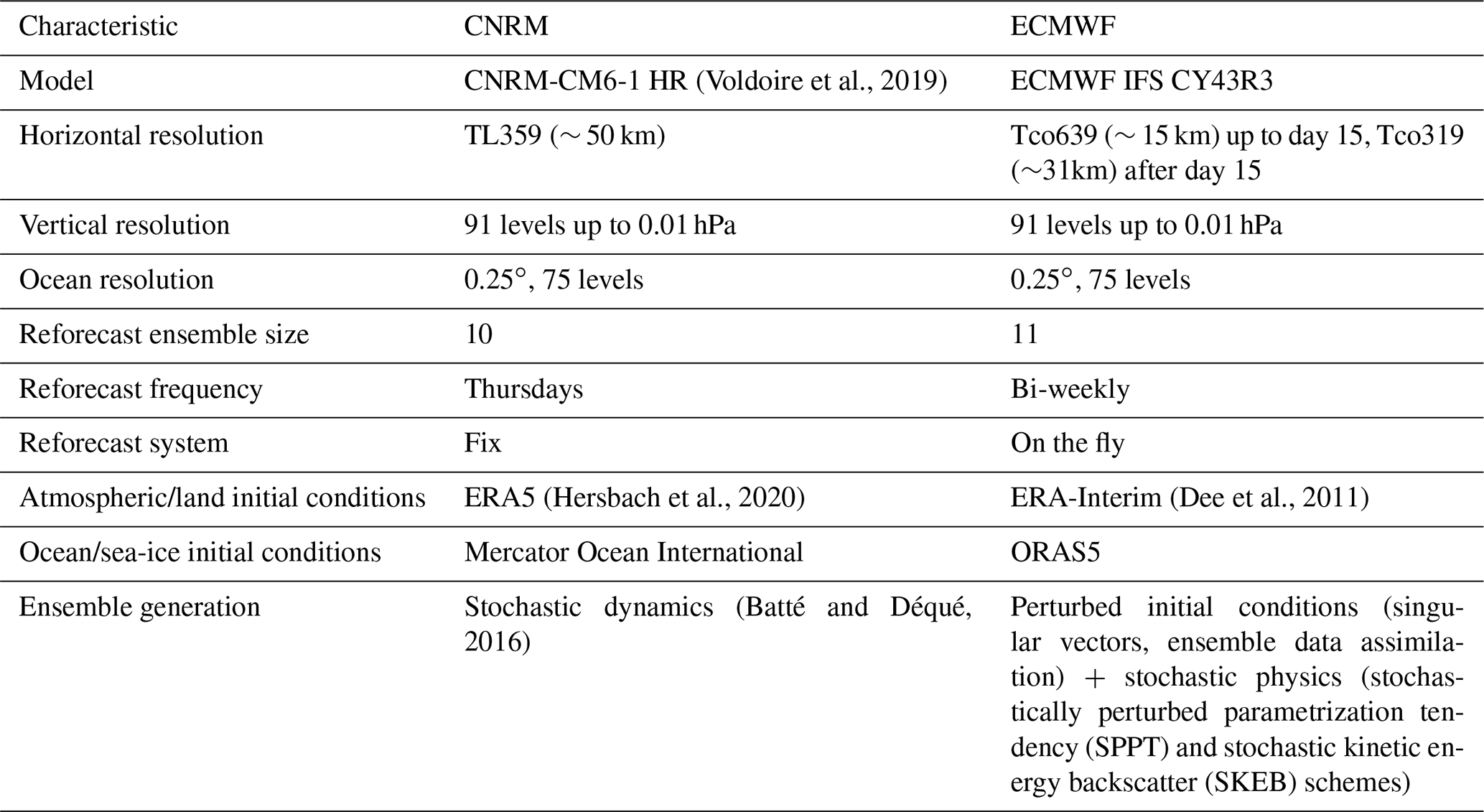
In this paper, “reforecast” and “forecast” indistinctly refer to retrospective forecasts, also named “hindcast” in other studies. The comparison of ECMWF and CNRM prediction systems is facilitated by their comparable reforecast ensemble size and a common 20-year reforecast period. Here, we consider the December-to-March extended winters from 1997/1998 to 2016/2017.

However, because of different reforecast designs, initial dates do not exactly match between the two systems. This issue is addressed as follows. We first select for each winter 16 consecutive CNRM start dates (i.e., Thursdays) after 13 November so that week 3 and 4 are always included within the December-to-March 4-month period. Then for each of these 320 (16×20) CNRM initial dates, we pick the closest date among the available ECMWF initial dates. Since ECMWF forecasts are issued twice a week, the resulting date from this selection either matches the CNRM counterpart or precedes or follows it by no more than 2 d, depending on the reforecast year. Note that each reforecast is evaluated against the corresponding reanalysis dates to ensure a perfectly fair inter-model comparison.

Forecast and observed daily anomalies are considered rather than full fields in order to remove the model bias: for the nth 32 d forecast (n≤16) of a given winter, daily anomalies are computed by subtracting the 32 d climatology as a function of lead time, corresponding to the mean of the nth forecasts of the 19 other winters.

In this study, we follow a frequently used convention in the S2S community to define weekly lead times (e.g., Vitart, 2004; Specq et al., 2020; de Andrade et al., 2021): week 1 goes from day 5 to day 11, week 2 from day 12 to 18, week 3 from day 19 to 25 and week 4 from day 26 to 32.

For the composite analysis described in Sect. 3.3.1, in addition to the forecast systems, we make use of a 300-year-long pre-industrial simulation (known as piControl) of the same model used in the CNRM system, namely CNRM-CM6-1-HR, and performed in the framework of the Coupled Model Intercomparison Project Phase 6 (CMIP6; Eyring et al., 2016). This experiment is useful to assess the behavior of the model internal variability without any drift from initial conditions nor forcing interference stemming from either initialization or volcanic and anthropogenic aerosols as well as greenhouse gas emissions. Additionally, this simulation provides enough years to work on densely populated composite samples, thereby ensuring an enhanced robustness of the results.

2.2 Reference dataset and forecast skill metrics

The ERA5 reanalysis (Hersbach et al., 2020) serves as the reference for daily sea-level pressure and daily mean 2 m temperature. This reanalysis, although resulting from a model output, assimilates a wide array of observations and will therefore be considered as our observational reference. For simplicity, we use the term “observation” – albeit loosely – to refer to ERA5 in the rest of the paper. Because ERA5 and ECMWF reforecasts are derived from two versions of the same model, one may object that ERA5 is not a suitable reference for this study. To verify if the assessment of the ECMWF predictions is favored by the choice of this reanalysis, we have compared some of the results obtained with ERA5 to results using the JRA-55 (Kobayashi et al., 2015) reanalysis as a reference. Given the very limited differences found (not shown), we have chosen to pursue the study with ERA5 only.

A common score to evaluate a subseasonal forecast system is the pointwise Pearson correlation between the ensemble mean forecasts and the corresponding observations over the entire reforecast period. Grid point time correlation is a classic deterministic score, whose significance is here determined by a two-sided Student t test at the 95 % confidence level.

In order to evaluate the skill of an individual forecast, we also compute the anomaly correlation coefficient (ACC), which shows the level of spatial agreement between the forecast and observed patterns. This is performed over a domain covering Europe (hereafter EUR; 34^∘ N–65^∘ N, 12^∘ W–41^∘ E). The domain boundaries are displayed on the map of Fig. 1. For ACCs, the significance is obtained by a bootstrapping method applied to the ensemble members of the forecasts: we compute the ACCs of 100 draws among the 10 (11) members of the CNRM (ECMWF) forecast and consider the forecast skillful if at least 95 % of the 100 ACCs exceed zero. For the sake of convenience, our definition of skillful individual forecasts is arbitrary and should be understood as “forecasts with the highest ACCs”. It does not imply that they systematically outperform climatological forecasts. This point is addressed by means of the probabilistic skill evaluation (see below). The root mean square error (RMSE) measuring the distance between the ensemble mean forecast and observation regardless of the sign of the anomaly has also been computed for individual forecasts and normalized by the interquartile range of the observation. However, this score has only been used to confirm a result found with the ACC in Sect. 3.1.

In addition to deterministic scores, the ensemble forecasts can be evaluated by means of probabilistic skill metrics. The continuous ranked probability score (CRPS) is the quadratic difference between the cumulative distribution function (CDF) of an ensemble forecast and the empirical CDF of the observation. The smaller the CRPS, the more accurate the forecast. Let F(x) be the forecast CDF for the variable x (e.g., weekly mean 2 m temperature) and y the corresponding observation; then the analytical expression of the CRPS is

$$\begin{array}{}\text{(1)}& \mathrm{CRPS}=\underset{\mathbb{R}}{\int }\left(F\right(x)-\mathbb{1}(x\ge y){)}^{\mathrm{2}}\mathrm{d}x,\end{array}$$

where 𝟙 is the indicator function.

It is also insightful to compute a continuous ranked probability skill score (CRPSS) for a dynamical forecast system by comparing its CRPS (CRPS_f) with that of a climatological forecast (CRPS_c) so that

$$\begin{array}{}\text{(2)}& \mathrm{CRPSS}=\mathrm{1}-{\displaystyle \frac{{\mathrm{CRPS}}_{\mathrm{f}}}{{\mathrm{CRPS}}_{\mathrm{c}}}}.\end{array}$$

CRPSS ranges between −∞ and 1, 1 corresponding to a perfect forecast. Negative CRPSS values indicate that dynamical forecasts are less accurate than climatological forecasts. In this study, we consider 16 forecasts per winter over 20 years. Therefore, for the nth (n≤16) forecast of a given year, the corresponding climatological forecast consists of a 19-member ensemble forecast grouping the nth forecasts of the 19 other years. To take into account the differences in ensemble size between the forecasts and their corresponding climatological forecasts, a so-called “fair” version of the CRPSS is computed via an unbiased estimator for the score that would be obtained as the ensemble size increases to infinity (Ferro et al., 2008; Ferro, 2014).

2.3 Weather regimes and NAO index

The computation of weather regimes is performed on the ERA5 1979–2017 extended winter, i.e., the months of November to March (hereafter NDJFM). It consists of a k-means clustering of daily maps of sea-level pressure (SLP) anomalies of the North Atlantic Europe (NAE) domain defined by the boundaries 20^∘ N–80^∘ N, 90^∘ W–30^∘ E. In order to facilitate this clustering, an empirical orthogonal function (EOF) analysis is applied to the SLP anomaly maps, for which the 19 leading modes are retained, explaining more than 90 % of the SLP variance. The four resulting clusters correspond to the typical North Atlantic weather regimes widely described and used in the literature (e.g., Michelangeli et al., 1995). By decreasing order of frequency, these regimes are identified as positive phase of the North Atlantic oscillation (NAO+), Scandinavian blocking (BLO), negative phase of the North Atlantic oscillation (NAO-) and Atlantic Ridge (AR). Each winter day of the reanalysis and the model simulations is then assigned to the weather regime for which the root mean square distance between the regime centroid and the map of SLP anomaly is minimal. Note that in this study, we have also tested a similar approach with a regime persistence criterion. More precisely, only sequences of 3 d or more corresponding to the same weather regime are effectively assigned to this regime. The impact of this persistence criterion is discussed at the end of Sect. 3.2.

The assessment of teleconnections is facilitated by the use of a NAO index that quantifies this oscillation. Here, it is calculated as the normalized time series of the first principal component, resulting from the projection of the daily ERA5 SLP anomaly field on the leading EOF. For further robustness and because there are multiple ways to define the NAO (Pokorná and Huth, 2015), a comparison is made with another NAO index computed independently by the US National Oceanic and Atmospheric Administration (NOAA) (NOAA Climate Prediction Center NAO index, 2020) on 500  hPa geopotential height fields from the NCEP/NCAR reanalysis and using a different method (Barnston and Livezey, 1987). Despite the many differences between the two daily NAO indices, their correlation for NDJFM 1979–2017 is as high as 0.77.

3 Results

In this section, we start with a general skill assessment to obtain a compared overview of the model ability to predict 2 m temperature at the subseasonal horizon. The second and third subsections address the question of flow dependence and the consequences on the forecast skill.

3.1 Skill of the subseasonal forecast systems

3.1.1 Northern Hemisphere assessment

The pointwise Pearson correlation between forecasts and observation is shown for week 1 to week 4 forecast times in Fig. 1.

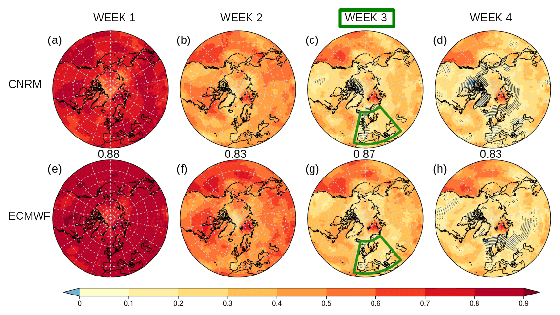
Figure 1 Correlation between 2 m temperature forecasts from week 1 to week 4 and the corresponding observation for CNRM (a–d) and ECMWF (e–h) forecast systems. Stippling indicates grid points where correlation is not significantly positive at the 95 % confidence level. The numbers show the spatial correlation between CNRM and ECMWF maps for each week. Green boxes indicate the focus region (EUR) and forecast lead time (week 3) targeted in Sect. 3.1.2.

It clearly shows for both systems the sharp decrease in skill after week 1 and also the better performance of the ECMWF system for the 4 weeks. This result was somehow expected given the much finer spatial resolution of the ECMWF system (Vitart, 2017). The skill difference could also originate from the better fit between the ECMWF forecast system and the ERA-Interim initial conditions, derived from another version of the same IFS model, in particular for the land surface slow-evolving components such as snow cover, soil moisture and deep soil temperature. Nonetheless, discussing the impact on skill of ECMWF and CNRM modeling and forecasting strategies is out of the scope of this study.

For both models, the correlation at week 3 remains positive for large parts of the Northern Hemisphere extratropics, albeit weakly over continents. At week 3 and 4, the ECMWF forecasts still show significant correlation over most of Europe, while this is only true over eastern Europe for CNRM. Overall, while ECMWF exhibits higher skill than CNRM, the large-scale patterns of grid point correlation are strikingly similar between both models, as confirmed by the high values of spatial correlations reported in Fig. 1.

However, positive correlations do not guarantee that these forecasts are more useful than a simple climatological forecast. To document this issue, we compare the CRPS probabilistic score with that of a climatological forecast by means of the fair CRPSS (see Sect. 2.2). On these maps (Fig. 2), white and blue shadings indicate regions where the forecasts do not perform better than the climatology. This score highlights the much better performance of ECMWF over CNRM as early as week 2. The skill patterns look like those found in the correlation analysis, but they are more drastic. For example at week 3, over Europe, the CNRM system shows only remnant skill near the Baltic Sea and the ECMWF over the north of the continent as well as a limited portion of central Europe. The contrast between the two systems is even more striking over North America. The comparatively poor CRPSS of CNRM could be the consequence of a lack of ensemble spread, resulting in a too-narrow distribution of forecasts, which denotes overconfident predictions. The complementary analysis shown in Appendix A, which compares the intra-ensemble standard deviation of the two systems from week 1 to week 4, tends to confirm this hypothesis.

Interestingly, the systems remain relatively skillful over the Mediterranean Sea but also the Sea of Okhotsk and the Kara, Barents and Labrador seas as well as, to a certain extent, the Baltic Sea. This could be a consequence of persisting sea-surface temperature (for the Mediterranean) and sea-ice extent (for the Arctic and North Atlantic seas) anomalies leading to enhanced subseasonal predictability of the near-surface atmosphere (Chevallier et al., 2019; Bach et al., 2019), although indisputable evidence would require a dedicated study.

From now on, our work focuses on the predictability of week 3 only.

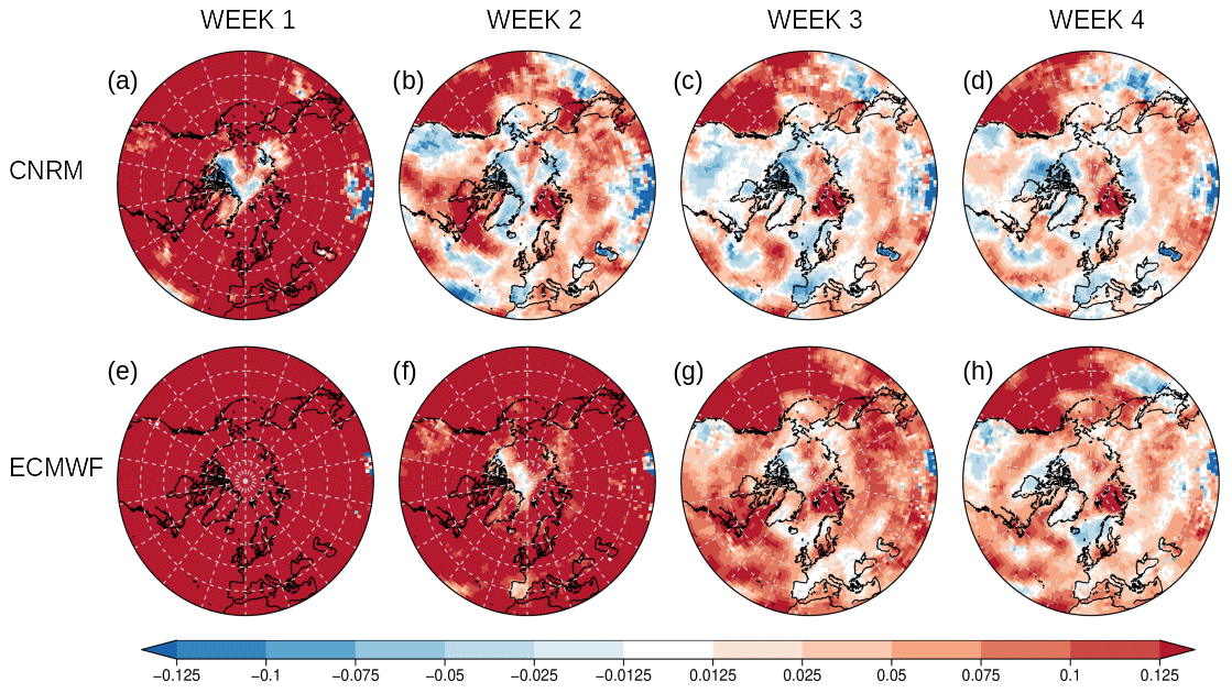
Figure 2 Fair CRPSS for week 1 to week 4 forecasts for CNRM (a–d) and ECMWF (e–h) forecast systems against climatological forecasts (see text). Red shade indicates that the actual forecasts are more skillful than the climatological counterparts.

3.1.2 Focus on Europe

The forecast skill of EUR 2 m temperature is assessed from the 320 reforecasts at week 3 for both systems by means of the ACC. This score varies considerably between dates. Thus, in order to investigate the degree of consistency between models' forecast skill, Fig. 3 plots the distribution of ECMWF ACC against CNRM ACC over EUR for each of the reforecast dates. Dots depict the 320 reforecasts and filled contours the corresponding probability density function. Red dots show the reforecasts where ACCs are significant at the 95 % level for both systems. This distribution is fairly symmetric, albeit slightly skewed towards higher values for ECMWF, which is consistent with results found in the previous section. This is also revealed by the mean and median points (black and gray triangles, respectively), located slightly above the y=x identity line. The standard deviation of ACCs is similar (0.42 for CNRM vs. 0.40 for ECMWF). More interestingly, the correlation between CNRM and ECMWF ACCs reaches 0.52. The correlation is even higher (0.61) when considering the RMSE of the individual forecasts instead of the ACC (not shown). The scatterplot also reveals that the most skillful concurrent forecasts (red dots) are less scattered and more grouped along the y=x identity line than other forecasts that are more spread out. They correspond to the maximum of the probability density function, plotted in green and yellow shades. This suggests that high-skill forecasts contribute more to the correlation than low-skill counterparts. In other words, CNRM and ECMWF systems are more prone to issue concurrently good forecasts than concurrently poor ones.

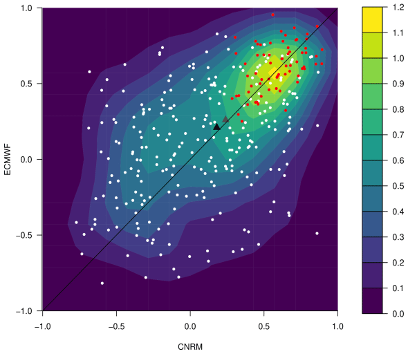
Figure 3 Scatterplot (dots) and probability density function (contours) of ECMWF ACC as a function of the corresponding CNRM ACC for each of the 320 wintertime reforecasts of EUR 2 m temperature at week 3. Red dots mark ACCs significant at the 95 % confidence level for both CNRM and ECMWF. The black and gray triangles correspond to the mean and the median point, respectively, and the solid black line to the y=x identity line.

The synchronicity found in the level of skill between the CNRM and ECMWF week 3 forecasts therefore indicates the existence of a common source of predictability concerning the EUR region.

We now investigate the distribution of skillful forecasts along the 20-year period considered in this study. The bar plots in Fig. 4 show a relatively consistent interannual variability: the number of yearly skillful forecasts for ECMWF, in red, is significantly correlated to that of CNRM, in blue (r=0.61). We reprocessed Figs. 3 and 4 after removing a linear trend derived from the DJFM ERA5 2 m temperature averaged over the Europe domain. We found no significant changes in the ACC distribution and correlation (0.519 instead of 0.521), nor in the interannual variability in skillful forecasts (not shown). Limited changes in the number of significantly positive ACCs per year and per forecast system before and after detrending confirm the minimal influence of the warming trend on the forecast skill.

In any case, 2009–2010 stands out as the winter with the maximum number of skillful forecasts of the 20-year period for both CNRM and ECMWF systems considered either jointly (green bars) or separately (blue and red bars). Since that winter is characterized by a record-breaking negative NAO index (Cattiaux et al., 2010), we have computed the correlation between the yearly number of skillful forecasts and a winter mean NAO index (December to March) derived from our daily NAO index datasets. The correlation is not significant if the NAO index is computed by averaging daily NAO indices (not shown). However, when computed as the mean of daily absolute values of the ERA5 NAO index (broken brown line in Fig. 4), the correlation found is significant. This is also true with the NOAA NAO index, with r ranging from 0.44 to 0.66. This result suggests that S2S EUR forecasts are more frequently skillful during winters characterized by a strong NAO index, either positive or negative.

Figure 4 Yearly number of skillful forecasts for CNRM (blue), ECMWF (red) and both systems (green) computed on EUR week 3 temperature forecasts. The broken brown line shows the absolute value of the winter NAO index derived from ERA5 (see text). The “r” values reported in the legend correspond to the correlation of this index with the yearly number of skillful forecasts.

Therefore, the next section focuses more specifically on the relationship between forecast skill and weather regimes.

3.2 Relationship between forecast skill and initial weather regime

We now consider the first 4 d after initialization as a relevant time window to discuss the initial weather regime. We argue that the choice of using 4 d instead of the single first day allows more robustness since the latter may sometimes lie in between two different regimes. This 4 d window is also consistent with the S2S convention that defines the first forecast week as starting from day 5 onwards (see Sect. 2.1).

We count separately for each member the occurrence of each weather regime assigned to the first 4 d of the forecast members, among the 68 EUR forecasts out of 320, that are concurrently skillful for CNRM and ECMWF.

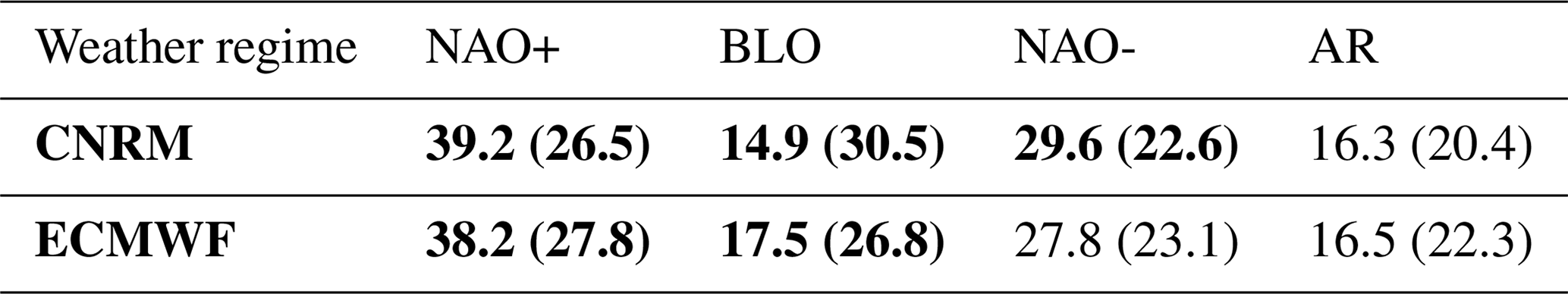
In this sample of 68 skillful reforecasts, the frequency of initial NAO+ days is significantly higher and that of initial BLO days lower than in the 252 other reforecasts for both forecast systems (Table 2). The frequency of NAO- initial days is also higher in CNRM but not significantly for ECMWF.

Table 2 Initial weather regime frequency in percent of skillful forecasts over EUR. Numbers in parentheses indicate the frequency for all the other forecasts. Bold characters highlight where the regime frequencies of skillful forecasts are significantly different from those in parentheses at the 95 % confidence level as determined by the bootstrapping method.

If skillful forecasts tend to start more frequently with NAO conditions, we would like to verify the reciprocal, i.e., how skillful the forecasts starting with NAO conditions are. To this end, instead of subsampling the forecasts according to their level of skill, we now cluster the 320 forecasts in four groups determined by their initial weather regime and compare the mean skill evolution along the forecast time for each of these clusters (Fig. 5). We define the initial weather regime of each forecast as the regime with the greatest number of occurrence during the 4 initial days.

Here the significance level is obtained by means of a bootstrapping method. More precisely, for a cluster of size N, a probability density function of mean ACC is built out of 1000 draws with replacement of N forecasts within this cluster. The forecast is then considered significant if the first percentile of the distribution is positive.

Figure 5 Mean ACC evolution with forecast time over Europe by initial weather regime for (a) CNRM and (b) ECMWF. Solid lines indicate values significantly positive at the 99 % confidence level. The number of forecasts for each initial regime is reported in parentheses.

For both systems, the mean ACC of the forecasts initialized in NAO+ conditions becomes higher than those initialized with other regimes by day 6 and more markedly from day 15 onwards, albeit not significantly (not shown). The difference vanishes past day 25 for CNRM but not for ECMWF. Finally, the ACC remains significantly positive until the end of the forecast period in both systems, although a positive ACC does not necessarily imply that the forecasts are useful, as discussed in Sect. 3.1. It is also interesting to notice that NAO- conditions do not lead to particularly skillful forecasts at week 3 for CNRM, as could have been expected from Table 2, and that models agree upon AR being the worst initial weather regime in terms of temperature subseasonal predictability over Europe since the mean ACC of forecasts initialized thereby are no longer significant past day 18 or 19.

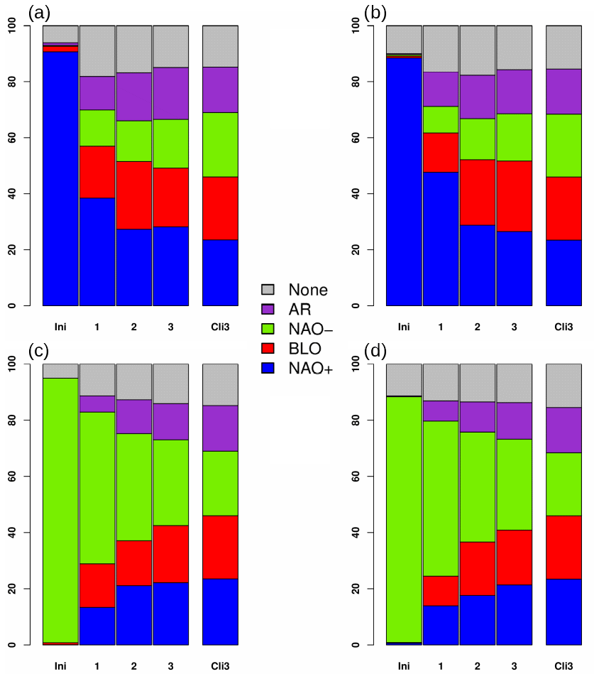
The next question arising from the previous results is the evolution in time of the regime frequency among these forecasts initiated under NAO+ or NAO- conditions. The stacked bar plots in Fig. 6 illustrate this evolution. Note that the residual non-NAO+ (resp. non-NAO-) regimes showing in the 4 initial days simply result from our clustering method based on the predominant regime counted within the 4 initial days of all ensemble members, thereby leaving some room for the occurrence of other weather regimes. We find that despite a rapid decrease in the NAO+ regime proportion with forecast time, it remains slightly larger than the climatological one at week 3. A similar but more pronounced result is found for NAO-. This suggests that the NAO regimes are persistent in the forecasts, although this cannot be ascertained at this stage since no statistical significance test has been performed here, and furthermore, all the ensemble members are pooled together, which conceals the transitions between weather regimes.

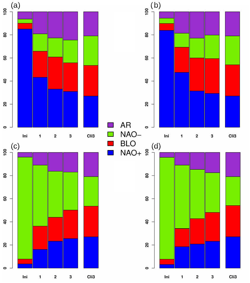
Figure 6 Weekly evolution of regime frequency among forecasts initialized in NAO+ (a) or NAO- (c) conditions for CNRM. (b, d) Same as (a) and (c) for ECMWF. The leftmost bar corresponds to the 4 initial days. The rightmost bar corresponds to the climatological frequency for week 3.

Before exploring further the causes of the above results, we need to address in more detail the question of regime persistence. So far, every forecast or observed day has been assigned with one of the four weather regimes, regardless of the day-to-day variability in the regime sequence. Such variability occurs when the spatial distribution of high- and low-pressure systems of a given day does not match well any of the canonical weather regimes or corresponds to a transition between two of them. To overcome this issue, we have defined a fifth category (called “none”) assigned to days outside any sequence of 3 or more days belonging to the same weather regime. Excluding the forecasts initialized with the predominant “none” category results in four smaller clusters of forecasts. Nonetheless the mean ACC evolution is not dramatically changed, and the ACC dependence on the initial conditions leads to the same hierarchy of weather regimes as can be seen in Appendix B. Similar conclusions can be drawn regarding the weekly evolution of regime frequency after taking the “none” category into account. Given the limited impact of the screening based on regime persistence, the following sections rely on the original daily weather regime assignment, i.e., without the “none” category.

3.3 Evidence of a lagged teleconnection

3.3.1 Composite analysis

The previous section has pinpointed a slight distortion in the weather regimes' distribution at week 3 for forecasts initialized in NAO conditions. For a broader comprehension, we thus compute the spatial composites of week 3 anomalies for this subset of forecasts for sea-level pressure (Fig. 7a and b) and 2 m temperature (Fig. 7e and f). Given that 87 (93) forecasts out of 320 are concerned for CNRM (ECMWF) and that each of them comprises 10 (11) members, the composite maps result from the average of n=870 (n=1027) single realizations. The ECMWF and CNRM composites show some similarities over the Atlantic sector with a distinct low-pressure anomaly over the Arctic and high-pressure anomaly centers near the Azores archipelago. The temperature patterns are even closer to each other with a large-scale warm anomaly stretching from central Europe to eastern Siberia and a cold anomaly over Canada, more pronounced near the Labrador Sea. The main difference between ECMWF and CNRM concerns the sea-level pressure anomaly over Europe, while there is no such discrepancy in terms of temperature anomaly. If we consider the positive pressure anomaly over the North Pacific, it may remind of the Arctic Oscillation (AO) loading pattern (e.g., Fig. 1 in Thompson and Wallace, 1998), although this anomaly is not significant for CNRM and more importantly not consistent with observations (see below).

The patterns found could be specific to the forecast systems, i.e., general circulation models (GCMs) constrained by imposed initial conditions and external forcing affected by a strong anthropogenic imprint. To verify this hypothesis, we derive a set of single-member pseudo-forecasts from the CNRM-CM6-1-HR 300-year-long piControl simulation. For each simulated year, we extract sixteen 32 d time series starting every 7 d from 13 November to 26 February so as to mimic successive S2S forecast start dates. Among the 4784 resulting pseudo-forecasts, those having a majority of initial days assigned as NAO+ are sampled to compute sea-level pressure and 2 m temperature anomaly composites (Fig. 7c and g). In this case, it concerns n= 957 realizations. We proceed likewise for the 1950–2017 ERA5 reanalysis (Fig. 7d and h) in order to compare the realism of this behavior with respect to observation. This long ERA5 period is a trade-off between a sufficient sample size, requiring more than 20 years to be comparable with reforecast composites, and a stable structure of weather regimes given the decadal variations in the NAO (e.g., Jung et al., 2003; Woollings et al., 2015). However, despite long-term shifts in the center of actions occurring during the 1950–2017 period, the main features of NAO regimes, characterized by the Eurasia–Canada temperature dipole and a North Atlantic meridional pressure gradient, are preserved.

The piControl composite shows broadly consistent patterns over the mid-Atlantic notwithstanding differences in terms of relative amplitude and extent of pressure anomalies. For temperature, the warm anomaly over the southeastern US is somewhat stronger than in the forecast systems. The amplitude of the ERA5 composite patterns is generally larger, which is at least partly explained by the reduced size of the composite sample (n=203). This observational composite shows a larger extent of the Atlantic high-pressure belt also covers southern Europe and central Asia and conversely no high-pressure anomaly over the North Pacific, which diverges from the hemispheric positive AO loading pattern evoked earlier. In terms of temperature, the main difference is the greater extent of the warm anomaly over North America and the cold pattern near the Bering Strait with respect to the forecast and piControl composites.

A similar composite analysis has been carried out with (pseudo-)forecasts initiated in NAO- (Fig. 8). Here the pressure and temperature composites show even more similarities between forecasts and observation, in particular over the North Atlantic Europe region. Similar to NAO+, surface pressure patterns show more differences than temperature, in particular over eastern Siberia, the western Pacific and North America. In the piControl composite, again, the patterns found are less intense but very consistent for temperatures and less so for surface pressure. One explanation for this reduced consistency could be that in the piControl time series, boundary conditions such as the ocean, sea ice and stratosphere also influencing the atmospheric flow have no reason to be coherent with observation, unlike the forecast composites initialized with reanalyzed atmospheric boundary conditions.

To summarize, this composite study reveals some significant agreement between forecast systems, unforced GCM and reanalysis concerning the prevailing atmospheric flow and near-surface temperature anomalies during the third week following NAO conditions. This agreement is much better for negative than positive NAO; for temperature than pressure patterns; and for the North Atlantic (pressure), Labrador, Europe and Siberia (temperature) regions. The lesser agreement found for NAO+ could relate to our clustering methodology, as discussed in the conclusion.

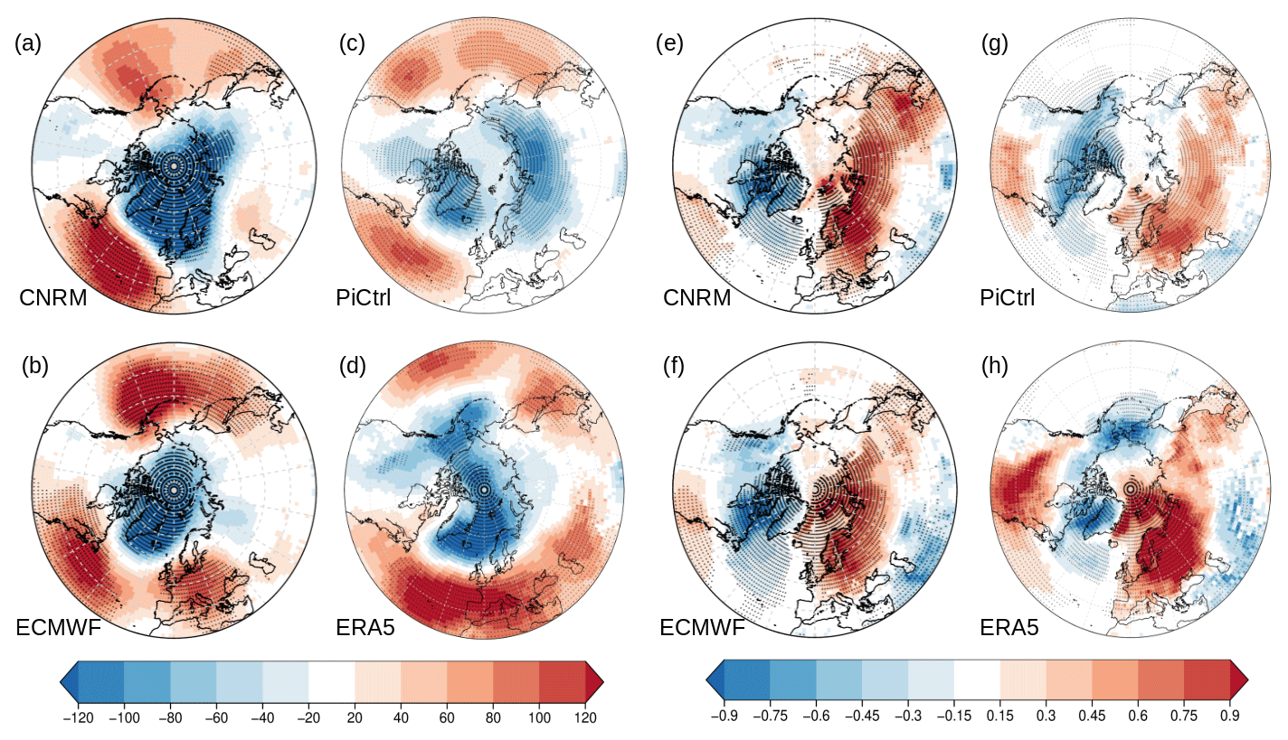
Figure 7 Composite anomaly of week 3 sea-level pressure (in pascals) following NAO+ initial conditions in (a) CNRM forecasts (n= 870), (b) ECMWF forecasts (n= 1027), (c) CNRM piControl pseudo-forecasts (n= 957) and (d) ERA5 reanalysis (n= 203). (e–h) Like (a)–(d) for 2 m temperature (in kelvin) initial conditions. Anomalies statistically significant at the 95 % level are stippled.

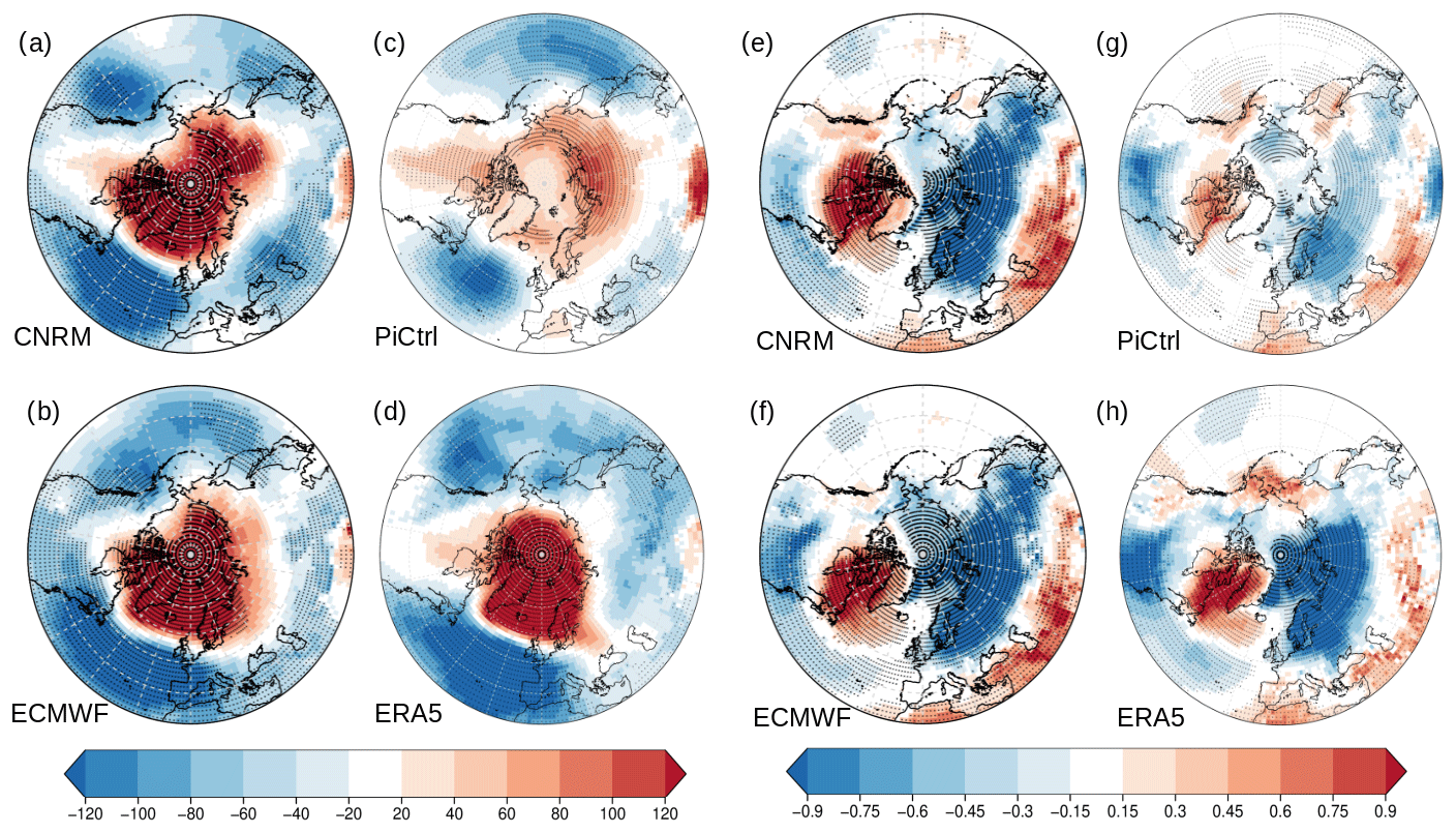
Figure 8 Same as Fig. 7 for NAO- initial conditions.

3.3.2 Observational NAO index

At this point, our study has only considered a weather regime assignment based on a root mean square distance criterion, but this method may conceal a wide array of atmospheric situations. Here we make use of the NAO index that quantifies the amplitude of the oscillation and allows periods of intense NAO+ or NAO- conditions to be identified. The composite analysis suggests that NAO initial conditions lead to NAO-like atmospheric flow. To verify this, we evaluate the extent to which the NAO index decorrelates with time in the observation. More precisely, Fig. 9 depicts the correlation of the averaged day-1-to-day-4 NAO index with a sliding window of 7 d running mean NAO index. The gray line and envelope consider the 608 aforementioned time series (that is, 16 per winter of the 1979–2017 period), whereas the red counterparts only consider the 10 % characterized by the highest absolute value of the initial NAO index. Such screening selects the time series with an initial atmospheric flow characterized by intense NAO+ and NAO- conditions. Despite different datasets and methodology, the NAO decorrelation compares well to other studies when keeping the whole sample (Keeley et al., 2009), with a characteristic decorrelation time of 8 to 10 d. However, the decorrelation is much slower when considering only the subsample with intense NAO initial conditions. Keeley et al. (2009) also identified a similar “shoulder” or “rebound” in the NAO decorrelation function between 10 and 30 d and find it largely related to interannual variability as opposed to intraseasonal. The decorrelation timescale and behavior are consistent when evaluated over a wide range of different NAO indices (Fig. 3b in Domeisen et al., 2018). The overlap between confidence intervals indicates that the difference found is not significant beyond 10 d when the NAO index is derived from ERA5 sea-level pressure. However it remains largely significant for the NOAA NAO index based on 500 hPa geopotential height, in particular 3 weeks after initialization where the correlation peaks up. For that matter, the sensitivity of NAO persistence to the NAO index definition is consistent with previous findings (Domeisen et al., 2018). Regardless of the NAO index calculation method, our results provide observational evidence of a long-lasting persistence of NAO-like atmospheric flow in winter.

Figure 9 Correlation and 95 % confidence interval (solid line and envelope) of initial NAO index with weekly running mean NAO index derived from (a) ERA5 and (b) NOAA. Gray (red) shades consider the full sample (subsample with intense NAO initial conditions) of time series within the 1979–2017 wintertime period, as described in the text. The $\mathrm{1}/e$ decorrelation threshold is marked with the dashed horizontal line.

Finally, still with this observational subsample of ERA5 time series characterized by intense “NAO-like” initial conditions, we regress the week three-pointwise 2 m temperature onto the initial NAO index (Fig. 10). Whether derived from ERA5 or NOAA, the patterns show similarities, with a stretch of positive correlation extending from the southeastern US to Siberia with maximum values near the Baltic Sea and two negative correlation lobes over Greenland and the Labrador Sea and from the tropical North Atlantic to North Africa and the Middle East.

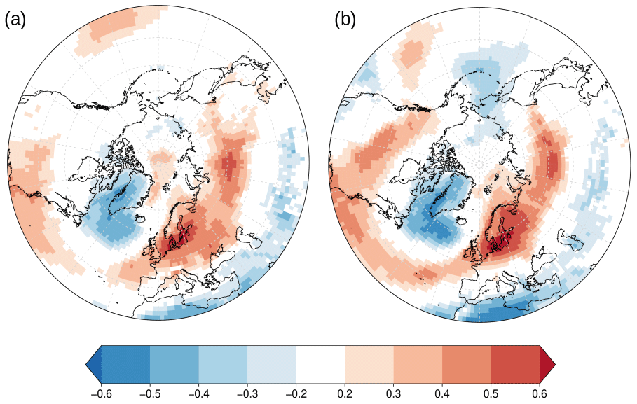
Figure 10 Correlation of ERA5 2 m temperature of week 3 with initial NAO index derived from (a) ERA5 or (b) NOAA. Only values significantly different from zero at the 99 % confidence level are displayed.

Given that the spatial extent of these correlation patterns encompasses large parts of the Northern Hemisphere, we now evaluate if NAO initial conditions of winter subseasonal forecasts could translate into enhanced prediction skill beyond Europe and how this relates to the regression patterns described above.

3.4 Consequences on forecast skill outside Europe

In the previous section, we identify a statistical link between wintertime temperature anomalies over a number of regions of the Northern Hemisphere extratropics and the NAO index 3 weeks prior. We now return to the forecast skill evaluation, but this time, we proceed to a subsampling of the reforecasts based on two conditions: the initial weather regime and its intensity. More precisely, we select all the reforecasts initiated in NAO+ and NAO- and evaluate their initial NAO index from the NOAA dataset. We then retain only the “initial NAO+” (“initial NAO-”) reforecasts for which the initial NAO index belongs to the upper (lower) quartile of the distribution. The choice of this percentile results from a trade-off between the strength of the initial NAO signal and a sufficient sample size. Figure 11 shows the week 2 m temperature correlation of week 3 after subsampling and the correlation difference with respect to the full sample of reforecasts (see Fig. 1c and g). The correlation patterns are patchier than in Fig. 1 because the sample size is considerably reduced, that is, 40 reforecasts instead of 320 for each system. Nonetheless, the correlation difference highlights a significantly increased skill over northwestern Europe and central Siberia as well as the Labrador Sea and the southeastern Mediterranean and Middle East to a lesser extent. These regions match remarkably well with the regression patterns highlighted in observations (Fig. 10), and they are relatively consistent between CNRM and ECMWF systems. Note that these regression patterns do not necessarily imply a causal relationship and may originate from a number of remote drivers (which are not investigated here). Indeed, no improvement of skill is detected over the southeastern US and off the US Atlantic coast.

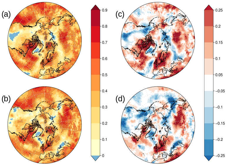
Figure 11 Correlation between the 2 m temperature of week 3 and the corresponding observation for the NAO initialized CNRM (a) and ECMWF (b) reforecasts. Panels (c) and (d) depict the correlation difference (a)  minus Fig. 1c for CNRM and (b) minus Fig. 1g for ECMWF. Stippling indicates significant values at the 95 % confidence level.

Even if there is no one-to-one relationship between local increase or decrease in the prediction skill and the aforementioned regression patterns, our study reveals consistent evidence that the forecast systems are capable of capturing the lagged NAO relationship to a certain extent. This provides additional subseasonal predictability at the continent scale, conditioned by the initial atmospheric flow.

In an attempt to better understand if the increased skill following intense NAO conditions was due to extended regime persistence or rather enhanced regime occurrence, we have performed additional analyses, reported and discussed in the Supplement to this study. Although these analyses only marginally elucidate the question, they suggest that forecasts initiated in strong NAO- conditions tend to have more persistent NAO- patterns in both CNRM and ECMWF. There is no such evidence for the NAO+ case. It could be that strong NAO+ initial conditions are followed by an increased recurrence of the NAO+ regime along the forecast time, but this feature is only found – arguably not very distinctly – in ECMWF.

4 Conclusions

The main objective of this study is to determine if the atmospheric circulation pattern in place at the time of initialization can impact the subseasonal predictive skill of forecasts delivered by state-of-the-art forecast systems. This study focuses on winter Northern Hemisphere extratropics near-surface temperature reforecasts issued by the new CNRM subseasonal forecast system as well as the ECMWF extended-range forecast system.

A first general skill assessment shows that the CNRM system proves less skillful than the ECMWF counterpart when considering the first 4 weeks after initialization, but the spatial patterns compare relatively well. The ensemble spread of the CNRM forecasts is too weak over much of the Northern Hemisphere across all the prediction horizons, which likely penalizes this system in terms of probabilistic skill.

When considering the performances of individual successive forecasts over Europe, the level of skill at week 3 tends to vary concurrently for both systems, thereby suggesting that they benefit from a common and intermittent source of subseasonal predictability. Since the European climate is known to be influenced by the North Atlantic Oscillation (NAO), a weather regime approach has provided evidence that forecasts initialized during positive NAO phases are slightly more skillful over Europe than those issued during the other three North Atlantic weather regimes.

A composite analysis has shown that temperature and sea-level pressure anomalies typical of the positive (negative) NAO regimes tend to characterize the third week following the occurrence of such a regime. This feature is well captured and comparable to a certain extent in forecasts, pre-industrial climate simulations and observations, particularly for temperature anomalies. The robustness of this time-lagged weather regime impact is further confirmed by the strong and persisting autocorrelation of the upper and lower tail of the NAO index distribution.

Ultimately, we show that the subseasonal predictive skill over Europe is more pre-conditioned by intense NAO events, either positive or negative, than by the prevailing regime at initialization. We also find that this flow-dependent skill concerns mostly northern Europe, but also central Siberia and regions surrounding the Labrador Sea.

In a next study, it would be worth studying the atmospheric mechanisms involved in this NAO lagged teleconnection and the extent to which they are properly captured by forecast systems. Such an approach could bring insight about the reasons why the NAO-initiated forecasts do not show improved skill over most of eastern North America, as could have been expected (Luo et al., 2020). At least for the coastal area, recent findings from Roberts et al. (2021) indicate that the skill could be improved by reducing the North Atlantic sea surface temperature biases resulting from inadequate representation of mesoscale ocean eddies in coupled models. Factors influencing the persistence of NAO+ and NAO- phases should also be investigated to go a step further into the concept of flow-dependent “windows of opportunity” for subseasonal prediction. In particular the influence of sudden stratospheric warming events on the occurrence and persistence of the NAO- regime has been evidenced (Domeisen, 2019). Hence, subseasonal forecasts issued after the onset of such events and characterized by a strong initial NAO phase could be even more trustworthy, although this hypothesis would require a large reforecast dataset to be verified.

Another prospect for future works would be to evaluate the sensitivity of the results to the methodology. First, our strategy to identify wintertime weather regimes, although widely referenced in the literature, may not be optimal (Falkena et al., 2020; Dorrington and Strommen, 2020). It could be that our clustering of the North Atlantic circulation into four weather regimes leads to NAO+ not being a mode of variability specific enough: it can be seen as a mere generic mode that potentially mixes a variety of distinct weather regimes. The robustness of our results would be worth assessing when considering a larger or smaller set of weather regimes. Then, the reforecast clustering strategy could also be questioned. In particular, a distance threshold between sea-level pressure patterns in reforecasts and the weather regime centroids could be applied in order to subsample only those reforecasts initiated in conditions very close the canonical modes of atmospheric variability.

Finally, including more forecast systems for a multi-model approach would bring considerable interest but also a great deal of additional complexity, given the many differences in the design of the S2S forecast systems.

Appendix A: Comparison of the CNRM and ECMWF ensemble spread

Figure A1 shows the weekly evolution with lead time of the intra-ensemble standard deviation of the 2 m temperature for the CNRM and the ECMWF subseasonal reforecasts. Since the CNRM ensemble size holds 10 members vs. 11 members for ECMWF, only 10 members of the latter have been used to guarantee a fair comparison of the two systems. The week-by-week differences (bottom row maps) help visualize that the ECMWF ensemble is more dispersive (red shades) than the CNRM counterpart over the vast majority of the Northern Hemisphere, whatever the prediction horizon. Only the North Pole and to a certain extent South Asia at longer lead times show more spread for CNRM. This lack of spread for CNRM is particularly pronounced over high-latitude continents, but considering the slow evolution of sea-surface temperature, the lack of spread over oceans is also meaningful and should not be overlooked.

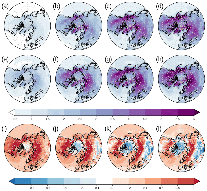
Figure A1 Ensemble standard deviation of 2 m temperature for week 1 to week 4 (a–d) CNRM and (e–h) ECMWF and week 1 to week 4 standard deviation differences “ECMWF minus CNRM” (i–l). Differences not significant at the 95 % confidence level have been set to zero.

Appendix B: Approach based on persisting regimes

We here provide the results obtained after taking into account the persistence of the weather regimes, resulting in a new category “none” (see Sect. 3.2 for details). As can be seen when comparing Fig. B1 with Fig. 5 and Fig. B2 with Fig. 6, the results found are very similar with or without this new category.

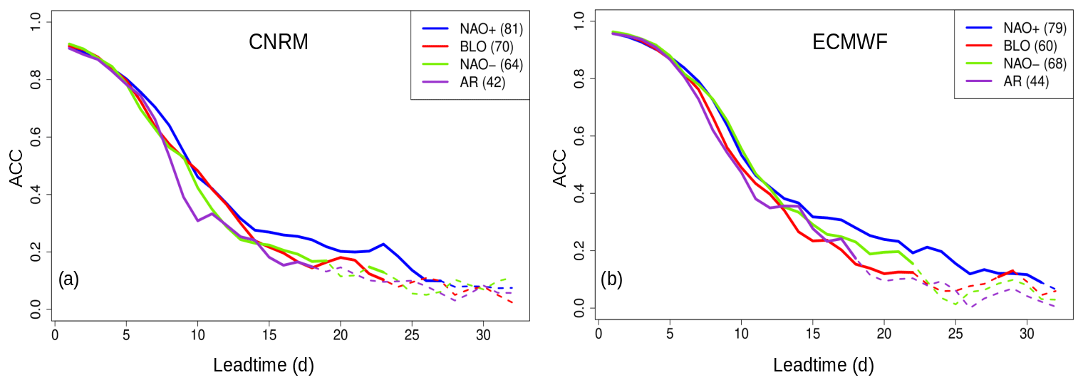
Figure B1 Like Fig. 5 but with a fifth category “none” including days outside any persistent sequence of a canonical weather regime.

Figure B2 Like Fig. 6 but with a fifth category “none” including days outside any persistent sequence of a canonical weather regime.